Comparison of Temperature-Dependent Hadronic Current Correlation Functions Calculated in Lattice Simulations of QCD and with a Chiral Lagrangian Model

Abstract

The Euclidean-time hadronic current correlation functions, $G_{P}(\tau,T)$ and $G_{V}(\tau,T)$, of pseudoscalar and vector currents have recently been calculated in lattice simulations of QCD and have been used to obtain the corresponding spectral functions. We have used the Nambu-Jona-Lasinio (NJL) model to calculate such spectral functions, as well as the Euclidean-time correlators, and have made a comparison to the lattice results for the correlators. We find evidence for the type of temperature dependence of the NJL coupling parameters that we have used in previous studies of the mesonic confinement-deconfinement transition. We also see that the spectral functions obtained when using the maximum-entropy-method (MEM) and the lattice data differ from the spectral functions that we calculate in our chiral model. However, our results for the Euclidean-time correlators are in general agreement with the lattice results, with better agreement when our temperature-dependent coupling parameters are used than when temperature-independent parameters are used for the NJL model. We also discuss some additional evidence for the utility of temperature-dependent coupling parameters for the NJL model. For example, if the constituent quark mass at $T=0$ is $352\,\mbox{MeV}$ in the chiral limit, the transition temperature is $T_{c}=208\,\mbox{MeV}$ for the NJL model with a standard momentum cutoff parameter. (If a Gaussian momentum cutoff is used, we find $T_{c}=225\,\mbox{MeV}$ in the chiral limit, with $m=368\,\mbox{MeV}$ at $T=0$.) The introduction of a weak temperature dependence for the coupling constant will move the value of $T_{c}$ into the range 150-170 MeV, which is more in accord with what is found in lattice simulations of QCD with dynamical quarks.

I INTRODUCTION

Euclidean-time hadronic current correlation functions contain information about the hadronic spectrum, including information about the temperature dependence of hadronic masses, the widths of these states and the eventual disappearance of such status from the spectrum at sufficiently high temperature. We have been interested in recent calculations of spectral functions of hadronic current correlators [ 1-3 ]. These calculations make use of lattice results for the Euclidean-time correlation functions, $G_{P}(\tau,T)$ and $G_{V}(\tau,T)$, of pseudoscalar and vector currents. For example, for the pseudoscalar correlator, one considers the equation

$$G_{P}(\tau,T)=\int_{0}^{\infty}d\omega\sigma_{P}(\omega,T)K(\tau,\omega,T)\,,$$ (1.1)

with

$$K(\tau,\omega,T)=\frac{\cosh[\omega(\tau-1/2T)]}{\sinh(\omega/2T)}\,,$$ (1.2)

and attempts to obtain values of the spectral function $\sigma_{P}(\omega,T)$ by using the maximum-entropy-method (MEM) [ 4, 5 ]. (A similar procedure is used to obtain $\sigma_{V}(\omega,T)$.) The MEM method is used, since the inversion of Eq. (1.1) to obtain $\sigma_{P}(\omega,T)$ is an ”ill-conditioned problem”[ 2 ], given the limitations of the lattice data.

The necessity of using such advanced numerical procedures is discussed in Ref. [ 2 ]. As stated there, one has to introduce assumptions as to the characteristics of the desired solutions when using the MEM analysis. At this point, the physical significance of the results for the spectral functions obtained with the MEM procedure is uncertain in the case of resonant structures with energies of several GeV found using that method.

Recently we have made some calculations of hadronic current correlators and their associated spectral functions [ 6 ]. Once we calculate the spectral functions using the Nambu-Jona-Lasinio (NJL) model, we may obtain $G_{P}(\tau,T)$ and $G_{V}(\tau,T)$ by using Eqs. (1.1) and (1.2). We may then compare our results for these Euclidean-time correlators with those calculated using the data obtained in the lattice simulations of QCD.

Since we have described our method of calculation of the spectral functions in an earlier work [ 6 ], we here relegate that material to the Appendix for ease of reference. A novel feature of our work is use of temperature-dependent coupling parameters for the NJL model. We have made use of such parameters in earlier studies of meson properties at finite temperature and have described the mesonic confinement-deconfinement transition [ 7 ]. While the use of temperature-dependent coupling constants for the NJL model is novel, we may note that the QCD coupling constant $\alpha_{s}$ has been made temperature-dependent in a study of the quark -gluon plasma equation of state in Ref. [ 8 ] and [ 9 ]. (See Fig. 1 of Ref. [ 9 ].) Values of the pressure, energy density and baryon density were presented as a function of temperature and quite good fits to QCD lattice results were obtained in Refs. [ 8 ] and [ 9 ].

In Ref. [ 6 ] we have introduced the spectral functions,

$$\sigma_{P}(\omega,T)=\frac{1}{\pi}\mbox{Im}C_{P}(\omega,T)\,,$$ (1.3)

and

$$\sigma_{V}(\omega,T)=\frac{1}{\pi}\mbox{Im}C_{V}(\omega,T)\,.$$ (1.4)

The relation between these functions and the ones that appear in the literature, $\overline{\sigma}_{P}(\omega,T)$ and $\overline{\sigma}_{V}(\omega,T)$ [ 1-3 ], is given in the Appendix. [ See Eqs. (A30) and (A31). ] In the Appendix we describe the procedures used in the calculation of $\mbox{Im}C_{P}(\omega,T)$ and $\mbox{Im}C_{V}(\omega,T)$.

The organization of our work is as follow. In Section II we present some of the results obtained for the functions $\mbox{Im}C_{P}(P_{0},T)/P_{0}^{2}$ and $\mbox{Im}C_{V}(P_{0},T)/P_{0}^{2}$. (We identify $P_{0}$ with $\omega$, which is used in the literature for the corresponding quantity.) In Section III and IV we compare the values of $G_{P}(\tau,T)$ and $G_{V}(\tau,T)$ obtained in our calculations and in the lattice simulations [ 2 ]. In those sections we discuss the evidence for the temperature-dependent coupling parameters we have used in other works [ 6, 7 ]. Finally, Section IV contains some additional discussion and conclusions.

II Euclidean-time Correlators of Pseudoscalar Hadronic Currents

The formalism reviewed in the Appendix is used to obtain the results presented in this section. In Fig.1 we show the values of $\mbox{Im}C_{P}(P_{0},T)/P_{0}^{2}$ that were first presented in Ref. [ 6 ]. The large peak at $T/T_{c}=1.2$ has its origin in the properties of a pion-like mode that is present after deconfinement has taken place. We note that no resonance is seen for $T/T_{c}=3.0$ [ dot-dashed line ], but resonance behavior is present for $T/T_{c}=1.5$ [ dashed line ] and $T/T_{c}=2.0$ [ dotted line ].

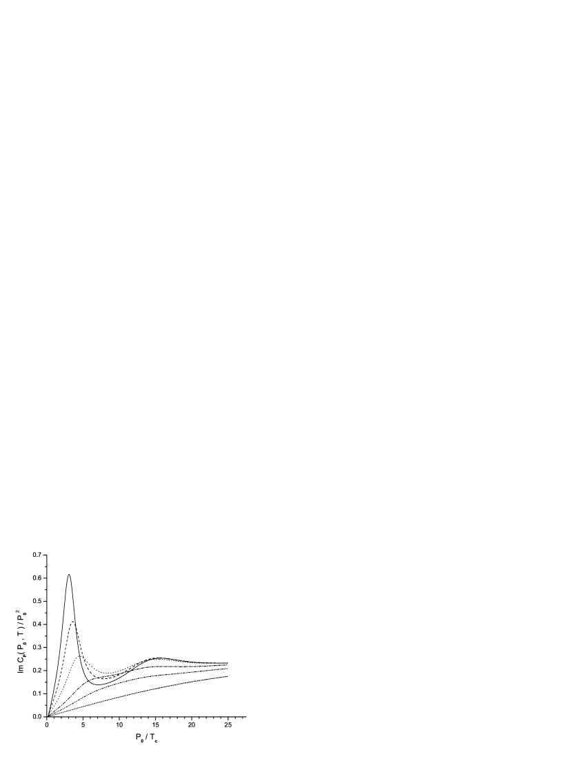
Figure 1: Values of $\mbox{Im}\,C_{P}(P_{0},T)/P_{0}^{2}$, obtained in Ref. [ 6 ], are shown for values of $T/T_{c}=1.2$ [ solid line ], $T/T_{c}=1.5$ [ dashed line ], $T/T_{c}=2.0$ [ dotted line ], $T/T_{c}=3.0$ [ dot-dashed line ], $T/T_{c}=4.0$ [ double dot-dashed line ], and $T/T_{c}=5.88$ [ short dashed line ]. Here we use $G_{P}(T)=G_{P}\,[\,1-0.17\,(T/T_{c})\,]$ with $T_{c}=0.150$ GeV and $G_{P}=13.49\,\mbox{GeV}^{-2}$.

Before we proceed, it is useful to discuss the properties of the integral in Eq. (1.1). We wish to show that the calculation of $G_{P}(\tau,T)$ is sensitive to the properties of $\sigma_{P}(\omega,T)$ for relatively small $\omega$, when $\tau T\sim 0.5$. On the other hand, when $\tau T$ is small (or near 1), the integral is sensitive to the values of $\sigma_{P}(\tau,T)$ for large $\omega$, where $\sigma_{P}(\tau,T)$ increases as $\omega^{2}$ and is largely model independent. These features may be seen in Fig.2, where the solid line represents our calculated values of $\sigma_{P}(\tau,T)=(1/\pi)\mbox{Im}C_{P}(\omega,T)$ for $T=1.5\,T_{c}$. The dashed line shows $K(\omega,\tau,T)$ for $\tau T=0.5$, while the dotted and dot-dashed lines show $K(\omega,\tau,T)$ for $\tau T=0.05$ and $\tau T=0.10$, respectively. We note that the $1/\omega$ singularity in $K(\omega,\tau,T)$ for small $\omega$ is compensated by the behavior of the spectral function at small $\omega$, $\sigma_{P}(\omega,T)\sim\omega$. These remarks also pertain to the calculation of $G_{V}(\tau,T)$ made using $\sigma_{V}(\omega,T)$.

Figure 2: Values of $K(\omega,\tau,T)$ are shown for $T=1.5\,T_{c}$ and $\tau T=0.05$ [ dotted line ], $\tau T=0.10$ [ dot-dashed line ], and $\tau T=0.50$ [ dashed line ]. The solid line represents $(1/\pi)\mbox{Im}C_{P}(\omega,T)$. Here, we use the notation $\omega=P_{0}$ and have put $T_{c}=0.150\,\mbox{GeV}$.

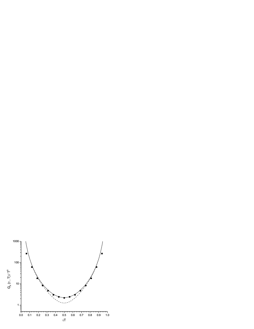
Figure 3: Values of $G_{P}(\tau,T)/T^{3}$ are shown as a function of $\tau T$, with $T=1.5\,T_{c}$. The solid line represents the result of our calculation made for $G_{P}(T)=G_{P}\,[\,1-0.17\,(T/T_{c})\,]$ with $G_{P}=13.49\,\mbox{GeV}^{-2}$. The dotted line is obtained when we use a constant value $G_{P}(T)=G_{P}$. The data (squares) are taken from Ref. [ 2 ] for the case $T=1.5\,T_{c}$.

Figure 4: Values of $G_{P}(\tau,T)/T^{3}$ are shown as a function of $\tau T$, for $T=3.0\,T_{c}$. The solid line is the result of our calculation made for $G_{P}(T)=G_{P}\,[\,1-0.17\,(T/T_{c})\,]$ with $G_{P}=13.49\,\mbox{GeV}^{-2}$, while the dotted line is obtained when we put $G_{P}(T)=G_{P}$. The data (squares) are taken from Ref. [ 2 ] for the case $T=1.5\,T_{c}$.

Figure 5: Values of $G_{P}(\tau,T)/T^{3}$ are shown for $T=3.0\,T_{c}$. Here the solid line is the same as the dashed line in Fig. 4 and corresponds to $G_{P}=0$. The dotted line is obtained when we use the constant value $G_{P}(T)=G_{P}=13.49\,\mbox{GeV}^{-2}$.

In Fig. 3 we show the data we have taken from Ref. [ 2 ] as squares. The solid line shows the result of our calculation of $G_{P}(\tau,T)/T^{3}$, as obtained from our calculated values of $\sigma_{P}(\omega,T)$ at $T=1.5\,T_{c}$. The deviation of our calculation from the data for $\tau T\simeq 0$ or $\tau T\simeq 1$ is inconsequential, given our remarks made in the previous paragraph. We also show the result for the case $G_{P}(T)=G_{P}=13.49\,\mbox{GeV}^{-2}$ as a dotted curve. When comparing the solid curve and the dotted curve we see evidence for the temperature dependence we have used: $G_{P}(T)=G_{P}[\,1-0.17(T/T_{c})\,]$. (We have obtained the value $G_{P}=13.49\,\mbox{GeV}^{-2}$ by calculating the pion mass at $T=0$ in our model.)

In Fig. 4 we show, as a solid line, our result for $G_{P}(\tau,T)/T^{3}$ at $T=3.0\,T_{c}$. In this case the fit to the data taken from Ref. [ 2 ] is poor. Therefore, we have investigated the case in which $G_{P}(T)=0$ and show the result as a dashed line in Fig. 4. The fit to the data of Ref. [ 2 ] is improved somewhat. We may suggest that the suppression of $G_{P}(T)$ at large temperatures may be greater than that given by the form we have used, $G_{P}(T)=G_{P}[\,1-0.17(T/T_{c})\,]$.

In Fig. 5 we again consider the value $T=3.0\,T_{c}$. In this case, the solid line is the result obtained when $G_{P}(T)=0$, while the dotted line results when we use a constant value for $G_{P}(T)=G_{P}=13.49\,\mbox{GeV}^{-2}$. We may compare our results for the spectral functions to those obtained using the MEM procedure and depicted in Ref. [ 2 ]. One essential difference is that we do not see the resonant behavior reported there for $T=3.0\,T_{c}$ at a rather high energy of about 2.4 GeV. The peak in $\overline{\sigma}_{P}(\omega,T)/\omega^{2}$ for $T=1.5\,T_{c}$ is at about 1 GeV in Ref. [ 2 ], while for $T=1.5\,T_{c}$ our peak in Fig. 1 is at about 0.55 GeV.

In estimating the energies of the peaks we have used $T_{c}=150$ MeV. However, if we use $T_{c}=270$ MeV, which is more appropriate for a lattice calculation without dynamical quarks, the resonant structures would appear at still higher energy.

III Euclidean-time Correlators of Lorentz-vector Hadronic Currents

Figure 6: Values of $\mbox{Im}\,C_{V}(P_{0},T)/P_{0}^{2}$, obtained in Ref. [ 6 ], are shown for values of $T/T_{c}=1.2$ [ solid line ], $T/T_{c}=1.5$ [ dashed line ], $T/T_{c}=2.0$ [ dotted line ], $T/T_{c}=3.0$ [ dot-dashed line ], $T/T_{c}=4.0$ [ double dot-dashed line ], and $T/T_{c}=5.88$ [ short dashed line ]. Here we use $G_{V}(T)=G_{V}\,[1-0.17\,(T/T_{c})]$ with $T_{c}=0.150$ GeV and $G_{V}=11.46\,\mbox{GeV}^{-2}$

Figure 7: Values of $(3/4)G_{V}(\tau,T)/T^{3}$ are shown for $T=1.5\,T_{c}$. Here, the solid line represents the result when we use $G_{V}(T)=G_{V}\,[\,1-0.17\,(T/T_{c})\,]$ with $G_{V}=11.46\,\mbox{GeV}^{-2}$. The dotted line is obtained when we use a constant value of $G_{V}(T)=G_{V}=11.46\,\mbox{GeV}^{-2}$. The data (squares) are taken from Ref. [ 2 ] for the case $T=1.5\,T_{c}$.

Figure 8: Values of $(3/4)G_{V}(\tau,T)/T^{3}$ are shown for $T=3.0\,T_{c}$. Here, the solid line represents the result when we use $G_{V}(T)=G_{V}\,[\,1-0.17\,(T/T_{c})\,]$ with $G_{V}=11.46\,\mbox{GeV}^{-2}$. The dotted line is obtained when we use a constant value of $G_{V}(T)=G_{V}=11.46\,\mbox{GeV}^{-2}$. The data (squares) are taken from Ref. [ 2 ] for the case $T=3.0\,T_{c}$.

We again refer to the Appendix for a review of our procedures for the calculation of the spectral functions from which we may obtain the Euclidean-time correlator using Eq. (1.1), with $\sigma_{V}(\omega,T)$ replacing $\sigma_{P}(\omega,T)$. In Fig. 6 we present our values of $\mbox{Im}C_{V}(P_{0},T)/P_{0}^{2}$, which may be compared to the values of $\overline{\sigma}_{V}(\omega,T)/\omega^{2}$ given in Fig. 1 of Ref. [ 2 ]. In Ref. [ 2 ] we find a peak at about 1 GeV for $T=1.5\,T_{c}$ and at about 2.5 GeV for $T=3.0\,T_{c}$. On the other hand, there is some weak resonant behavior seen for $T=1.5\,T_{c}$ [ dashed line ] in our Fig. 6 at about 0.75 GeV which may reflect a residual enhancement due to a $\rho$-like mode that is present after the confinement-deconfinement transition has taken place. At $T=3.0\,T_{c}$ [ dot-dashed line ], we see no resonance enhancement in our work, in contrast to what is obtained by the MEM analysis of Ref. [ 2 ].

In Fig. 7 we show the data taken from Ref. [ 2 ] as squares. Here, there is hardly any difference seen in the data reported for $T=1.5\,T_{c}$ and $T=3.0\,T_{c}$. In Fig. 7, the solid line represents our results for $(3/4)G_{V}(\tau,T)/T^{3}$ at $T=1.5\,T_{c}$. We only achieve a fair fit to the data, but the fit is decidedly better than that obtained when a constant value of $G_{V}(T)=G_{V}=11.46\,\mbox{GeV}^{-2}$ is used [ dotted line ] (See the appendix for a discussion of the factor 3/4 used when making comparison to the data of Ref. [ 2 ] in the case of vector current correlators.)

In Fig. 8 we compare our result for $(3/4)G_{V}(\tau,T)/T^{3}$ at $T=3.0\,T_{c}$ [ solid line ] with the data of Ref. [ 2 ]. Here the fit is better than that of Fig. 4. Again, the use of a constant value of $G_{V}(T)=G_{V}=11.46\,\mbox{GeV}^{-2}$ yields a poor result. We suggest that our analysis tends to support our choice of temperature-dependent coupling parameters for the NJL model.

IV discussion

It is of interest to obtain further insight into the results shown in Figs. 4 and 5. To that end, we show various calculations made for $\mbox{Im}C_{P}(P_{0},T)/P_{0}^{2}$ in Fig. 9. There, for $T=3.0\,T_{c}$, the solid line is the result of our model, the dotted curve corresponds to the use of a constant value of the coupling parameter $G_{P}(T)=G_{P}=13.49\,\mbox{GeV}^{-2}$, while the dashed line is the result for $G_{P}(T)=0$. A comparison of the solid curve and the dashed curve leads to some understanding of the results shown in Fig. 4, while a comparison of the dotted curve and the dashed curve leads to further understanding of the results shown in Fig. 5. Similar results are given for $\mbox{Im}C_{V}(P_{0},T)/P_{0}^{2}$ in Fig. 10. For that figure, a comparison of the solid curve and the dashed curve gives some insight into the results shown in Fig. 8, where the dotted line corresponds to $G_{V}(T)=G_{V}=11.46\,\mbox{GeV}^{-2}$ and the solid curve represents the results of our model.

We now return to the pseudoscalar case for $T=1.5\,T_{c}$. In Fig. 11 we show $\mbox{Im}C_{P}(P_{0},T)/P_{0}^{2}$ for our model [ solid line ], for $G_{P}(T)=0$ [dashed line], and for the case $G_{P}(T)=G_{P}=13.49\,\mbox{GeV}^{-2}$. We recall that our model, with the temperature-dependent coupling parameter, gave rise to a excellent fit to the data, as seen in Fig. 3. It is also of interest to present values of $\sigma_{P}(\omega,T)=(1/\pi)\mbox{Im}C_{P}(\omega,T)/\omega^{2}$ for $T=1.5\,T_{c}$. In Fig. 12, the result of our model is shown as a solid line, the dot-dashed line is for $G_{P}(T)=0$, and the dotted line is obtained when $G_{P}(T)=G_{P}=13.49\,\mbox{GeV}^{-2}$. It is seen, that for small values of $P_{0}$, on the whole, the dotted line lies below the other curves, giving rise to the behavior seen in Fig. 3 for $\tau T\simeq 0.5$.

It is worth mentioning that we have some additional evidence of the utility of temperature-dependent coupling parameters for the NJL model. We note that the confinement-deconfinement transition takes place in the range $150\,\mbox{MeV}\leq T_{c}\leq 170\,\mbox{MeV}$ for QCD with dynamical quarks. We then inspect Fig. 5 of Ref. [ 10 ], where the constituent quark mass of the NJL model is presented as a function of temperature for the case of a temperature-independent coupling constant. The mass value is $330\,\mbox{MeV}$ at $T=0$ and is about $260-300\,\mbox{MeV}$ when $150\,\mbox{MeV}\leq T\leq 170\,\mbox{MeV}$. Thus, we do not see the (partial) restoration of the chiral symmetry that is expected for $T\sim T_{c}$. On the other hand, we see in Fig. 1 of Ref. [ 7 ], where we have used a temperature-dependent coupling parameter, that we have $m_{u}=364\,\mbox{MeV}$ at $T=0$ and $m_{u}(T)$ in the range of 50 to $100\,\mbox{MeV}$ for $150\,\mbox{MeV}$ $\leq T\leq 170\,\mbox{MeV}$. That is much more in accord with the (partial) restoration of chiral symmetry when $T\sim T_{c}$. If we wish to consider the NJL as a useful low-energy model of QCD, it is much easier to discuss the confinement-deconfinement transition if we use temperature-dependent coupling parameters.

Figure 9: Values of $\mbox{Im}\,C_{P}(P_{0},T)/P_{0}^{2}$ are shown for $T=3.0\,T_{c}$. The solid line is the result of our model with temperature-dependent coupling parameters, the dotted line is obtained in the absence of the temperature dependence ($G_{P}(T)=G_{P}=13.49\,\mbox{GeV}^{-2}$), and the dashed line represents the result for $G_{P}(T)=0$.

Figure 10: Values of $\mbox{Im}\,C_{V}(P_{0},T)/P_{0}^{2}$ are shown for $T=3.0\,T_{c}$. The solid line is the result of our model with temperature-dependent coupling parameters, the dotted line is obtained in the absence of the temperature dependence ($G_{V}(T)=G_{V}=11.46\,\mbox{GeV}^{-2}$), and the dashed line represents the result for $G_{V}(T)=0$.

Figure 11: Values of $\mbox{Im}\,C_{P}(P_{0},T)/P_{0}^{2}$ are shown for $T=1.5\,T_{c}$. Here, the solid line is the result of our model, the dashed line represent the result for $G_{P}(T)=0$, while the dotted line is obtained when we use $G_{P}(T)=G_{P}=13.49\,\mbox{GeV}^{-2}$. [ See Fig. 3 for the values of $G_{P}(\tau,T)/T^{3}$ calculated for $T=1.5\,T_{c}$, using the values of $\mbox{Im}\,C_{P}(P_{0},T)/P_{0}^{2}$ shown here as the solid and dotted line. ]

Figure 12: Values of $\sigma_{P}(\omega,T)=(1/\pi)\mbox{Im}\,C_{P}(P_{0},T)$ are shown for $T=1.5\,T_{c}$. Here, the solid line corresponds to our model, with $G_{P}(T)=G_{P}\,[\,1-0.17\,(T/T_{c})\,]$, the dot-dashed line is obtained when $G_{P}(T)=0$, and the dashed line is for the case $G_{P}(T)=G_{P}=13.49\,\mbox{GeV}^{-2}$. (See Fig. 13.)

Figure 13: We exhibit the values of $m_{u}(T)$ obtained using Eq. (5.38) of Ref. [11], with $m^{0}=5.50\,\mbox{MeV}$ and $\Lambda=0.631\,\mbox{GeV}$. The dotted curve corresponds to the use of a constant value $G=5.691\,\mbox{GeV}^{-2}$, in the notation of Ref. [11]. For the solid and dashed curves we have used $G(T)=G\,[\,1-0.17(T/T_{c})\,]$. For the solid curve we have put $T_{c}=0.170\,\mbox{GeV}$, while for the dashed curve, we have used $T_{c}=0.150\,\mbox{GeV}$ in our parametrization of $G(T)$.

Figure 14: Values of $m_{u}(T)$ are shown. The dashed curve is calculated with $m^{0}=5.50\,\mbox{MeV}$. Here, $G(T)=G\,[\,1-0.17\,(T/T_{c})\,]$, with $G=5.691\,\mbox{GeV}^{-2}$ and $T_{c}=0.150\,\mbox{GeV}$. The solid curve is calculated with the same value of $G(T)$ and $T_{c}$, but with $m^{0}=0$. From the solid curve, we see that chiral symmetry is restored at $T=0.136\,\mbox{GeV}$ when $m^{0}=0$.

For ease of reference,we have calculated the constituent mass of the up quark using the equation for the temperature-dependent constituent mass given in Ref. [ 11 ]. We have used a current quark mass of $m^{0}=5.5\,\mbox{MeV}$ and a momentum cutoff of $\Lambda=0.631\,\mbox{GeV}$. In Fig. 13, the dotted curve shows the result obtained with $G=5.691\,\mbox{GeV}^{-2}$ (in the notation of Ref. [ 11 ]). From Fig. 13 we see that at $T=0.150\,\mbox{GeV}$, $m_{u}=0.318\,\mbox{GeV}$, while at $T=0.170\,\mbox{GeV}$, $m_{u}=0.276\,\mbox{GeV}$. The dashed and solid curves represent the result when $G(T)=G[\,1-0.17(T/T_{c})\,]$. For the solid curve ($T_{c}=0.170\,\mbox{GeV}$), $m_{u}=77\,\mbox{MeV}$ at $T=0.170\,\mbox{GeV}$. For the dashed curve ($T_{c}=0.150\,\mbox{GeV}$), $m_{u}=54\,\mbox{MeV}$ at $T=0.150\,\mbox{GeV}$. Again, we see that it is much easier to discuss the (partial) restoration of chiral symmetry at the confinement-deconfinement transition when we use the temperature-dependent coupling parameters of our model.

It is also of interest to exhibit the role played by the current quark mass. In Fig. 14, the dashed curve, which was calculated for $T_{c}=0.150\,\mbox{GeV}$, is the same as the dashed curve in Fig. 13. In Fig. 14, the solid curve shows the result when $m^{0}=0$. Here, we see restoration of chiral symmetry at $T=0.136\,\mbox{GeV}$, when $G(T)=G[\,1-0.17(T/T_{c})\,]$ with $T_{c}=0.150\,\mbox{GeV}$.

We note that the value of $T_{c}=0.136\,\mbox{GeV}$ is still within the uncertainty of the transition temperature for three-flavor QCD. For example, in Ref. [ 12 ] the transition temperatures are given for two-flavor and three-flavor QCD. In the latter case, $T_{c}=154\pm 8\,\mbox{MeV}$, with a suggested systematic error similar to the statistical error, so that $T_{c}=154\pm 8\pm 8\,\mbox{MeV}$ [ 12 ]. (We have used coupling constants determined in our studies of the three-flavor NJL model, so that consideration of the transition temperature for that case is appropriate.)

If we wish to assign a physical interpretation of the parameter $T_{c}$ in the expression for $G(T)$, we may use $G(T)=G[\,1-0.135(T/T_{c})\,]$ with $T_{c}=0.150\,\mbox{GeV}$. That choice gives rise to restoration of chiral symmetry at $T=T_{c}=0.150\,\mbox{GeV}$ in the NJL model with $m^{0}=0$. If we maintain the value $m^{0}=0$, but use a constant value for $G(T)=5.691\,\mbox{GeV}^{-2}$, with $\Lambda=0.631\,\mbox{GeV}$, we find restoration of chiral symmetry at $T_{c}=208\,\mbox{MeV}$.

The calculations reported in Fig. 13 and 14 may also be made using our Gaussian cutoff, $\mbox{exp}(-\overrightarrow{k}^{2}/\alpha^{2})$, with $\alpha=0.605\,\mbox{GeV}$. For example, we may consider the dashed curve of Fig. 14. If we use the Gaussian cutoff and use $G=6.004\,\mbox{GeV}^{-2}$, instead of $G=5.691\,\mbox{GeV}^{-2}$, we obtain a curve that is very close to the dashed curve of Fig. 14 for $T>0.080\,\mbox{GeV}$. However, the mass at $T=0$ is $382\,\mbox{MeV}$ instead of $364\,\mbox{MeV}$ which was the value obtained using the sharp cutoff of $\Lambda=0.631\,\mbox{GeV}$ and $G=5.691\,\mbox{GeV}^{-2}$.

We have performed what are essentially parameter-free calculations of hadronic spectral functions and have computed the corresponding Euclidean-time correlation functions. The values of the coupling parameters, $G_{S}$ and $G_{V}$, were fixed in calculations of meson properties at $T=0$. We have used the temperature dependence, $G(T)=G[\,1-0.17(T/T_{c})\,]$, which was introduced in earlier work in which we studied the (mesonic) confinement-deconfinement transition [ 7 ]. We believe it is of interest to see that we obtain reasonable values for the Euclidean correlators. Of more importance, however, is our observation that we find some evidence for the temperature dependence of the NJL coupling parameters that we have used in other works. By analogy, we expect that the coupling parameters should also be density-dependent, and we have introduced such density dependence in earlier work [ 13 ]. Density dependence of the coupling parameters may be particularly important, given the strong interest in diquark condensates and color superconductivity at high baryon density [ 14 ].

APPENDIX

For ease of reference, we present a discussion of our calculation of hadronic current correlators taken from Ref. [ 6 ]. The procedure we adopt is based upon the real-time finite-temperature formalism, in which the imaginary part of the polarization function may be calculated. Then, the real part of the function is obtained using a dispersion relation. The result we need for this work has been already given in the work of Kobes and Semenoff [ 15 ]. (In Ref. [ 15 ] the quark momentum in Fig. 2 is $k$ and the antiquark momentum is $k-P$. We will adopt that notation in this section for ease of reference to the results presented in Ref. [ 15 ].) With reference to Eq. (5.4) of Ref. [ 15 ], we write the imaginary part of the scalar polarization function as

$$\mbox{Im}\,J_{S}(\textit{P}\,{}^{2},T)=\frac{1}{2}(2N_{c})\beta_{S}\,\epsilon(\textit{P}\,{}^{0})\!\int\!\!\frac{d^{3}\!{k}}{(2\pi)^{3}}\,e^{-\vec{k}\,{}^{2}/\alpha^{2}}\left(\frac{2\pi}{2E_{1}(k)2E_{2}(k)}\right)$$ (A1)

$$\{(1-n_{1}(k)-n_{2}(k))\delta(\textit{P}\,{}^{0}-E_{1}(k)-E_{2}(k))$$

$$-(n_{1}(k)-n_{2}(k))\delta(\textit{P}\,{}^{0}+E_{1}(k)-E_{2}(k))$$

$$-(n_{2}(k)-n_{1}(k))\delta(\textit{P}\,{}^{0}-E_{1}(k)+E_{2}(k))$$

$$-(1-n_{1}(k)-n_{2}(k))\delta(\textit{P}\,{}^{0}+E_{1}(k)+E_{2}(k))\}\,.$$

Here, $E_{1}(k)=[\,\vec{k}\,{}^{2}+m_{1}^{2}(T)\,]^{1/2}$. Relative to Eq. (5.4) of Ref. [ 15 ], we have changed the sign, removed a factor of $g^{2}$ and have included a statistical factor of $2N_{c}$, where the factor of 2 arises from the flavor trace. In addition, we have included a Gaussian regulator, $\exp[\,-\vec{k}\,{}^{2}/\alpha^{2}\,]$, with $\alpha=0.605$ GeV, which is the same as that used in most of our applications of the NJL model in the calculation of meson properties. We also note that

$$n_{1}(k)=\frac{1}{e^{\,\beta E_{1}(k)}+1}\,,$$ (A2)

and

$$n_{2}(k)=\frac{1}{e^{\,\beta E_{2}(k)}+1}\,.$$ (A3)

For the calculation of the imaginary part of the polarization function, we may put $k^{2}=m_{1}^{2}(T)$ and $(k-P)^{2}=m_{2}^{2}(T)$, since in that calculation the quark and antiquark are on-mass-shell. In Eq. (A1) the factor $\beta_{S}$ arises from a trace involving Dirac matrices, such that

$$\beta_{S} = -\mbox{Tr}[\,(\hbox to0.0pt{\hbox to5.52084pt{\hfil/\hfil}\hss}k+m_{1})(\hbox to0.0pt{\hbox to5.52084pt{\hfil/\hfil}\hss}k-\hbox to0.0pt{\hbox to7.80904pt{\hfil/\hfil}\hss}P+m_{2})\,]$$ (A4)

$$= 2P^{2}-2(m_{1}+m_{2})^{2}\,,$$ (A5)

where $m_{1}$ and $m_{2}$ depend upon temperature. In the frame where $\vec{P}=0$, and in the case $m_{1}=m_{2}$, we have $\beta_{S}=2P_{0}^{2}(1-{4m^{2}}/{P_{0}^{2}})$. For the scalar case, with $m_{1}=m_{2}$, we find

$$\mbox{Im}\,J_{S}(P^{2},T)=\frac{N_{c}P_{0}^{2}}{4\pi}\left(1-\frac{4m^{2}(T)}{P_{0}^{2}}\right)^{3/2}e^{-\vec{k}\,{}^{2}/\alpha^{2}}[\,1-2n_{1}(k)\,]\,,$$ (A6)

where

$$\vec{k}\,{}^{2}=\frac{P_{0}^{2}}{4}-m^{2}(T)\,.$$ (A7)

For pseudoscalar mesons, we replace $\beta_{S}$ by

$$\beta_{P} = -\mbox{Tr}[\,i\gamma_{5}(\hbox to0.0pt{\hbox to5.52084pt{\hfil/\hfil}\hss}k+m_{1})i\gamma_{5}(\hbox to0.0pt{\hbox to5.52084pt{\hfil/\hfil}\hss}k-\hbox to0.0pt{\hbox to7.80904pt{\hfil/\hfil}\hss}P+m_{2})\,]$$ (A8)

$$= 2P^{2}-2(m_{1}-m_{2})^{2}\,,$$ (A9)

which for $m_{1}=m_{2}$ is $\beta_{P}=2P_{0}^{2}$ in the frame where $\vec{P}=0$. We find, for the $\pi$ mesons,

$$\mbox{Im}\,J_{P}(P^{2},T)=\frac{N_{c}P_{0}^{2}}{4\pi}\left(1-\frac{4m^{2}(T)}{P_{0}^{2}}\right)^{1/2}e^{-\vec{k}\,{}^{2}/\alpha^{2}}[\,1-2n_{1}(k)\,]\,,$$ (A10)

where $\vec{k}\,{}^{2}={P_{0}^{2}}/4-m_{u}^{2}(T)$, as above. Thus, we see that, relative to the scalar case, the phase space factor has an exponent of 1/2 corresponding to a s-wave amplitude. For the scalars, the exponent of the phase-space factor is 3/2, as seen in Eq. (A6).

For a study of vector mesons we consider

$$\beta_{\mu\nu}^{V}=\mbox{Tr}[\,\gamma_{\mu}(\hbox to0.0pt{\hbox to5.52084pt{\hfil/\hfil}\hss}k+m_{1})\gamma_{\nu}(\hbox to0.0pt{\hbox to5.52084pt{\hfil/\hfil}\hss}k-\hbox to0.0pt{\hbox to7.80904pt{\hfil/\hfil}\hss}P+m_{2})\,]\,,$$ (A11)

and calculate

$$g^{\mu\nu}\beta_{\mu\nu}^{V}=4[\,P^{2}-m_{1}^{2}-m_{2}^{2}+4m_{1}m_{2}\,]\,,$$ (A12)

which, in the equal-mass case, is equal to $4P_{0}^{2}+8m^{2}(T)$, when $m_{1}=m_{2}$ and $\vec{P}=0$. This result will be needed when we calculate the correlator of vector currents in the next section. Note that, for the elevated temperatures considered in this work, $m_{u}(T)=m_{d}(T)$ is quite small, so that $4P_{0}^{2}+8m_{u}^{2}(T)$ can be approximated by $4P_{0}^{2}$, when we consider the vector current correlation functions. In that case, we have

$$\mbox{Im}\,J_{V}(P^{2},T)\simeq\frac{2}{3}\mbox{Im}\,J_{P}(P^{2},T)\,.$$ (A13)

At this point it is useful to define functions that do not contain that Gaussian regulator:

$$\mbox{Im}\,\tilde{J}_{P}(P^{2},T)=\frac{N_{c}P_{0}^{2}}{4\pi}\left(1-\frac{4m^{2}(T)}{P_{0}^{2}}\right)^{1/2}[\,1-2n_{1}(k)\,]\,,$$ (A14)

and

$$\mbox{Im}\,\tilde{J}_{V}(P^{2},T)=\frac{2}{3}\frac{N_{c}P_{0}^{2}}{4\pi}\left(1-\frac{4m^{2}(T)}{P_{0}^{2}}\right)^{1/2}[\,1-2n_{1}(k)\,]\,,$$ (A15)

For the functions defined in Eq. (A14) and (A15) we need to use a twice-subtracted dispersion relation to obtain $\mbox{Re}\,\tilde{J}_{P}(P^{2},T)$, or $\mbox{Re}\,\tilde{J}_{V}(P^{2},T)$. For example,

$$\mbox{Re}\,\tilde{J}_{P}(P^{2},T)=\mbox{Re}\,\tilde{J}_{P}(0,T)+\frac{P^{2}}{P_{0}^{2}}[\,\mbox{Re}\,\tilde{J}_{P}(P_{0}^{2},T)-\mbox{Re}\,\tilde{J}_{P}(0,T)\,]+$$ (A16)

$$\frac{P^{2}(P^{2}-P_{0}^{2})}{\pi}\int_{4m^{2}(T)}^{\tilde{\Lambda}^{2}}ds\frac{\mbox{Im}\,\tilde{J}_{P}(s,T)}{s(P^{2}-s)(P_{0}^{2}-s)}\,,$$

where $\tilde{\Lambda}^{2}$ can be quite large, since the integral over the imaginary part of the polarization function is now convergent. We may introduce $\tilde{J}_{P}(P^{2},T)$ and $\tilde{J}_{V}(P^{2},T)$ as complex functions, since we now have both the real and imaginary parts of these functions. We note that the construction of either $\mbox{Re}\,J_{P}(P^{2},T)$, or $\mbox{Re}\,J_{V}(P^{2},T)$, by means of a dispersion relation does not require a subtraction. We use these functions to define the complex functions $J_{P}(P^{2},T)$ and $J_{V}(P^{2},T)$.

In order to make use of Eq. (A16), we need to specify $\tilde{J}_{P}(0)$ and $\tilde{J}_{P}(P_{0}^{2})$. We found it useful to take $P_{0}^{2}=-1.0$ GeV² and to put $\tilde{J}_{P}(0)=J_{P}(0)$ and $\tilde{J}_{P}(P_{0}^{2})=J_{P}(P_{0}^{2})$. The quantities $\tilde{J}_{V}(0)$ and $\tilde{J}_{V}(P_{0}^{2})$ are determined in an analogous function. This procedure in which we fix the behavior of a function such as $\mbox{Re}\tilde{J}_{V}(P^{2})$ or $\mbox{Re}\tilde{J}_{V}(P^{2})$ is quite analogous to the procedure used in Ref. [ 16 ]. In that work we made use of dispersion relations to construct a continuous vector-isovector current correlation function which had the correct perturbative behavior for large $P^{2}\rightarrow-\infty$ and also described that low-energy resonance present in the correlator due to the excitation of the $\rho$ meson. In Ref. [ 16 ] the NJL model was shown to provide a quite satisfactory description of the low-energy resonant behavior of the vector-isovector correlation function.

We now consider the calculation of temperature-dependent hadronic current correlation functions. The general form of the correlator is a transform of a time-ordered product of currents,

$$iC(P^{2},T)=\int d^{4}xe^{iP\cdot x}<\!\!<T(j(x)j(0))>\!\!>\,,$$ (A17)

where the double bracket is a reminder that we are considering the finite temperature case.

For the study of pseudoscalar states, we may consider currents of the form $j_{P,i}(x)=\tilde{q}(x)i\gamma_{5}\lambda^{i}q(x)$, where, in the case of the $\pi$ mesons, $i=1,2$ and $3$. For the study of scalar-isoscalar mesons, we introduce $j_{S,i}(x)=\tilde{q}(x)\lambda^{i}q(x)$, where $i=0$ for the flavor-singlet current and $i=8$ for the flavor-octet current [ 7 ].

In the case of the pseudoscalar-isovector mesons, the correlator may be expressed in terms of the basic vacuum polarization function of the NJL model, $J_{P}(P^{2},T)$ [ 11, 17, 18 ]. Thus,

$$C_{P}(P^{2},T)=J_{P}(P^{2},T)\frac{1}{1-G_{P}(T)J_{P}(P^{2},T)}\,,$$ (A18)

where $G_{P}(T)$ is the coupling constant appropriate for our study of $\pi$ mesons. We have found $G_{P}(T)=13.49$ GeV^-2 by fitting the pion mass in a calculation made at $T=0$, with $m_{u}=m_{d}=0.364$ GeV. The result given in Eq. (A18) is only expected to be useful for small $P^{2}$, since the Gaussian regulator strongly modifies the large $P^{2}$ behavior. Therefore, we suggest that the following form is useful, if we are to consider the larger values of $P^{2}$.

$$\frac{C_{P}(P^{2},T)}{P^{2}}=\left[\frac{\tilde{J}_{P}(P^{2},T)}{P^{2}}\right]\frac{1}{1-G_{P}(T)J_{P}(P^{2},T)}\,.$$ (A19)

(As usual, we put $\vec{P}=0$.) This form has two important features. At large $P_{0}^{2}$, ${\mbox{Im}\,C_{P}(P_{0},T)}/{P_{0}^{2}}$ is a constant, since ${\mbox{Im}\,\tilde{J}_{P}(P_{0}^{2},T)}$ is proportional to $P_{0}^{2}$. Further, the denominator of Eq. (A19) goes to 1 for large $P_{0}^{2}$. On the other hand, at small $P_{0}^{2}$, the denominator is capable of describing resonant enhancement of the correlation function. As we will see, the results obtained when Eq. (A19) is used appear quite satisfactory. ( We may again refer to Ref. [ 16 ], in which a similar approximation is described.)

For a study of the vector-isovector correlators, we introduce conserved vector currents $j_{\mu,i}(x)=\tilde{q}(x)\gamma_{\mu}\lambda_{i}q(x)$ with i=1, 2 and 3. In this case we define

$$J_{V}^{\mu\nu}(P^{2},T)=\left(g\,{}^{\mu\nu}-\frac{P\,{}^{\mu}P\,{}^{\nu}}{P^{2}}\right)J_{V}(P^{2},T)$$ (A20)

and

$$C_{V}^{\mu\nu}(P^{2},T)=\left(g\,{}^{\mu\nu}-\frac{P\,{}^{\mu}P\,{}^{\nu}}{P^{2}}\right)C_{V}(P^{2},T)\,,$$ (A21)

taking into account the fact that the current $j_{\mu,\,i}(x)$ is conserved. We may then use the fact that

$$J_{V}(P^{2},T)=\frac{1}{3}g_{\mu\nu}J_{V}^{\mu\nu}(P^{2},T)$$ (A22)

and

$$\mbox{Im}\,J_{V}(P^{2},T) = \frac{2}{3}\left[\frac{P_{0}^{2}+2m_{u}^{2}(T)}{4\pi}\right]\left(1-\frac{4m_{u}^{2}(T)}{P_{0}^{2}}\right)^{1/2}e^{-\vec{k}\,{}^{2}/\alpha^{2}}[\,1-2n_{1}(k)\,]$$ (A23)

$$\simeq \frac{2}{3}\mbox{Im}J_{P}(P^{2},T)\,.$$ (A24)

(See Eq. (A7) for the specification of $k=|\vec{k}|$.) We then have

$$C_{V}(P^{2},T)=\tilde{J}_{V}(P^{2},T)\frac{1}{1-G_{V}(T)J_{V}(P^{2},T)}\,,$$ (A25)

where we have introduced

$$\mbox{Im}\tilde{J}_{V}(P^{2},T) = \frac{2}{3}\left[\frac{P_{0}^{2}+2m_{u}^{2}(T)}{4\pi}\right]\left(1-\frac{4m_{u}^{2}(T)}{P_{0}^{2}}\right)^{1/2}[\,1-2n_{1}(k)\,]$$ (A26)

$$\simeq \frac{2}{3}\mbox{Im}\tilde{J}_{P}(P^{2},T)\,.$$ (A27)

In the literature, $\omega$ is used instead of $P_{0}$ [  1-3  ]. We may define the spectral functions

$$\sigma_{V}(\omega,T)=\frac{1}{\pi}\,\mbox{Im}\,C_{V}(\omega,T)\,,$$ (A28)

and

$$\sigma_{P}(\omega,T)=\frac{1}{\pi}\,\mbox{Im}\,C_{P}(\omega,T)\,,$$ (A29)

Since different conventions are used in the literature [ 1-3 ], we may use the notation $\overline{\sigma}_{P}(\omega,T)$ and $\overline{\sigma}_{V}(\omega,T)$ for the spectral functions given there. We have the following relations:

$$\overline{\sigma}_{P}(\omega,T)=\sigma_{P}(\omega,T)\,,$$ (A30)

and

$$\frac{\overline{\sigma}_{V}(\omega,T)}{2}=\frac{3}{4}\sigma_{V}(\omega,T)\,,$$ (A31)

where the factor 3/4 arises because, in Refs. [ 1-3 ], there is a division by 4, while we have divided by 3, as in Eq. (A22).

References

(1)I. Wetzorke, F. Karsch, E. Laermann, P. Petreczky, and S. Stickan, Nucl. Phys. Proc. Suppl.
106 ,510(2002)-hep-lat/0110132.
(2)F. Karsch, S. Datta, E. Laermann, P. Petreczky, and S. Stickan, and I. Wetzorke, hep-ph/0209028.
(3)F. Karsch, E.Laermann, P. Petreczky, S. Stickan, and I. Wetzorke, Phys. Lett. B 530, 147 (2002).
(4)M. Asakawa, T. Hatsuda and Y. Nakahara, Prog. Part. Nucl. Phys. 46, 459 (2001)
(5)Y. Nakahara, M. Asakawa and T. Hatsuda, Phys. Rev. D 60, 091503 (1999).
(6)Bing He, Hu Li, C. M. Shakin, and Qing Sun, hep-ph/0212345.
(7)Hu Li and C. M. Shakin, hep-ph/0209136.
(8)J. Letessier and J. Rafelski, hep-ph/0301099.
(9)S. Hamieh, J. Letessier and J. Rafelski, Phys. Rev. C 62, 064901 (2000).
(10)S. Schmidt, D. Blaschke and Y. L. Kalinovsky, Phys. Rev. C 50, 435 (1994).
(11)S. P. Klevansky, Rev. Mod. Phys. 64 ,649 (1992).
(12)F. Karsch, hep-ph/0106019.
(13)Hu Li and C. M. Shakin, Phys. Rev. D 66, 074016 (2002).
(14)For reviews, see K. Rajagopal and F. Wilczek, in
At the Frontier of Particle Physics/Handbook of QCD, M. Shifman ed.
(World Scientific, Singapore 2001); M. Alford, Annu. Rev. Nucl. Part. Sci.
51, 131 (2001).
For a recent application of NJL model in the calculation of the properties of dense matter, see
D. Blaschke, S. Fredrikesson, H. Grigorian, and A. M. Oztas, nucl-th/0301002.
(15)R. L. Kobes and G. W. Semenoff, Nucl. Phys. B 260, 714 (1985).
(16)C. M. Shakin, Wei-Dong Sun, and J. Szweda, Ann of Phys. (NY) 241, 37 (1995).
(17)T. Hatsuda and T. Kunihiro, Phys. Rep. 247, 221 (1994).