Abstract

We investigate the possibility of detecting solar electron antineutrinos with the KamLAND experiment. These electron antineutrinos are predicted by spin-flavor oscillations at a significant rate even if this mechanism is not the leading solution to the SNP.

KamLAND is sensitive to antineutrinos originated from solar ⁸B neutrinos. From KamLAND negative results after 145 days of data taking, we obtain model independent limits on the total flux of solar electron antineutrinos $\Phi({}^{8}B)<1.1-3.5\times 10^{4}\ cm^{-2}\ s^{-1}$, more than one order of magnitude smaller than existing limits, and on their appearance probability $P<0.15\%$ (95% CL).

Assuming a concrete model for antineutrino production by spin-flavor precession, this upper bound implies an upper limit on the product of the intrinsic neutrino magnetic moment and the value of the solar magnetic field $\mu B<2.3\times 10^{-21}$ MeV 95% CL (for LMA $(\Delta m^{2},\tan^{2}\theta)$ values).

Limits on neutrino transition moments are also obtained. For realistic values of other astrophysical solar parameters these upper limits would imply that the neutrino magnetic moment is constrained to be, in the most conservative case, $\mu\mbox{$\leq$}3.9\times 10^{-12}\ \mu_{B}$ (95% CL) for a relatively small field $B=50$ kG. For higher values of the magnetic field we obtain: $\mu\mbox{$\leq$}9.0\times 10^{-13}\ \mu_{B}$ for field $B=200$ kG and $\mu\mbox{$\leq$}2.0\times 10^{-13}\ \mu_{B}$ for field $B=1000$ kG at the same statistical significance.

PACS:

^⋆ e-mail: emilio.torrente-lujan@cern.ch.

Present address: Dept. Fisica, GFT. Universidad de Murcia. Murcia. Spain.

1 Introduction

Evidence of eelctron antineutrino disappearance in a beam of antineutrinos in the KamLAND experiment has been recently presented [1]. The analysis of these results [1, 2] in terms of neutrino oscillations have largely improved our knowledge of neutrino mixing in the LMA region. The results appear to confirm in a independent way that the observed deficit of solar neutrinos is indeed due to neutrino oscillations. The ability to measure the LMA solution, the one preferred by the solar neutrino data at present, “in the lab” puts KamLAND in a pioneering situation: after these results there should remain little doubt of the physical reality of neutrino mass and oscillations. Once neutrino mass is observed, neutrino magnetic moments are an inevitable consequence in the Standard Model and beyond. Magnetic moment interactions arise in any renormalizable gauge theory only as finite radiative corrections: the diagrams which contribute to the neutrino mass will inevitably generate a magnetic moment once the external photon line is added.

The KamLAND experiment is the successor of previous reactor experiments ( CHOOZ [3], PaloVerde [4]) at a much larger scale in terms of baseline distance and total incident flux. This experiment relies upon a 1 kton liquid scintillator detector located at the old, enlarged, Kamiokande site. It searches for the oscillation of antineutrinos emitted by several nuclear power plants in Japan. The nearby 16 (of a total of 51) nuclear power stations deliver a $\overline{\nu}_{e}$ flux of $1.3\times 10^{6}cm^{-2}s^{-1}$ for neutrino energies $E_{\nu}>1.8$ MeV at the detector position. About $85\%$ of this flux comes from reactors forming a well defined baseline of 139-344 km. Thus, the flight range is limited in spite of using several reactors, because of this fact the sensitivity of KamLAND increases by nearly two orders of magnitude compared to previous reactor experiments.

Beyond reactor neutrino measurements, the secondary physics program of KamLAND includes diverse objectives as the measurement of geoneutrino flux emitted by the radioactivity of the earth’s crust and mantle, the detection of antineutrino bursts from galactic supernova and, after extensive improvement of the detection sensitivity, the detection of low energy ${}^{7}Be$ neutrinos using neutrino-electron elastic scattering.

Moreover, the KamLAND experiment is capable of detecting potential electron antineutrinos produced on fly from solar ⁸B neutrinos [5]. These antineutrinos are predicted by spin-flavor oscillations at a significant rate if the neutrino is a Majorana particle and if its magnetic moment is high enough [6, 7]. In Ref.[5] as been remarked that the flux of reactor antineutrinos at the Kamiokande site is comparable, and in fact smaller, to the flux of ⁸B neutrinos emitted by the sun ,$\Phi({}^{8}B)\simeq 5.6\times 10^{6}cm^{-2}s^{-1}$ [1, 8, 9]. Their energy spectrum is important at energies $2-4$ MeV while solar neutrino spectrum peaks at around $9-10$ MeV. As the inverse beta decay reaction cross section increases as the square of the energy, we would expect nearly 10 times more solar electron antineutrino events even if the initial fluxes were equal in magnitude.

The publication of the SNO results [10, 9] has already made an important breakthrough towards the solution of the long standing solar neutrino [11, 12, 13, 14] problem (SNP) possible. These results provide the strongest evidence so far (at least until KamLAND improves its statistics) for flavor oscillation in the neutral lepton sector.

The existing bounds on solar electron antineutrinos are strict. The present upper limit on the absolute flux of solar antineutrinos originated from ${}^{8}B$ neutrinos is [5, 16, 17] $\Phi_{\overline{\nu}}({}^{8}B)<1.8\times 10^{5}\ cm^{-2}\ s^{-1}$ which is equivalent to an averaged conversion probability bound of $P<3.5\%$ (SSM-BP98 model). There are also bounds on their differential energy spectrum [16]: the conversion probability is smaller than $8\%$ for all $E_{e,vis}>6.5$ MeV going down the $5\%$ level above $E_{e,vis}\simeq 10$ MeV.

The main aim of this work is to study the implications of the recent KamLAND results on the determination of the solar electron antineutrino appearance probability, independently from concrete models on antineutrino production. The structure of this work is the following. In section 2 we discuss the main features of KamLAND experiment that are relevant for our analysis: The salient aspects of the procedure we are adopting and the results of our analysis are presented and discussed in sections 3. In Section 4 we apply the results we obtained in a particular model for the solar magnetic field, we obtain bounds on the values of the intrinsic neutrino transition magnetic moments. Finally, in section 5 we draw our conclusions and discuss possible future scenarios.

2 The computation of the expected signals

2.1 The KamLAND signal

Electron antineutrinos from any source, nuclear reactors or solar origin, with energies above 1.8 MeV are measured in KamLAND by detecting the inverse $\beta$-decay reaction $\overline{\nu}_{e}+p\to n+e^{+}$. The time coincidence, the space correlation and the energy balance between the positron signal and the 2.2 MeV $\gamma$-ray produced by the capture of a already-thermalized neutron on a free proton make it possible to identify this reaction unambiguously, even in the presence of a rather large background.

The two principal ingredients in the calculation of the expected signal in KamLAND are the corresponding flux and the electron antineutrino cross section on protons. The average number of positrons $N_{i}$ originated from the solar source which are detected per visible energy bin $\Delta E_{i}$ is given by the convolution of different quantities:

$$N_{i} = Q_{0}\int_{\Delta E_{i}}dE_{e}\int_{0}^{\infty}dE_{e}^{r}\epsilon(E_{e})R(E_{e},E_{e}^{r})\int_{E_{e}^{r}}^{\infty}dE_{\overline{\nu}}\overline{p}(E_{\overline{\nu}})\Phi(E_{\overline{\nu}})\sigma(E_{\overline{\nu}},E_{e}^{r})$$ (1)

where $Q_{0}$ is a normalization constant accounting for the fiducial volume and live time of the experiment, $\overline{p}$. Expressions for the electron antineutrino capture cross section $\sigma(E_{\overline{\nu}},E_{e}^{r})$ are taken from the literature [18, 19]. The matrix element for this cross section can be written in terms of the neutron half-life, we have used the latest published value $t_{1/2}=613.9\pm 0.55$ [17]. The functions $\epsilon(E_{e})$ and $R(E_{e},E_{e}^{r})$ are the detection efficiency and the energy resolution function. We use in our analysis the following expression for the energy resolution in the prompt positron detection $\sigma(E_{e})=0.0062+0.065\surd E_{e}$ . This expression is obtained from the raw calibration data presented in Ref.[20]. Note that we prefer to use this expression instead of the much less accurate one given in Ref.[1]. Moreover, we assume a 408 ton fiducial mass and the detection efficiency is taken independent of the energy [1], $\epsilon=80\%$. In order to obtain concrete limits, a model should be taken which predict $\overline{p}$ and its dependence with the energy. For our purpose it will suffice to suppose $\overline{p}$ a constant. This is justified at least in two cases: a) if the energy range $\Delta E$ over which we perfom the integration is small enough so the variation of the probability is not very large, or b) if we reinterpret ${\overline{p}}$ as an energy-averaged probability, note that, in a general case, this is always true because the un-avoidable convolution with a finite energy resolution. (see Expression 10 in Ref.[7]):

$${\overline{p}}_{\Delta E} = \int_{\Delta E}dE\ \sigma(E)\Phi(E)P_{\overline{\nu}}(E)/{\int_{\Delta E}dE\ \sigma(E)\Phi(E)}.$$ (2)

Let us finally note that independently of the reasons above, upper limits to be obtained on continuation are still valid even if the antineutrino probabilities are significantly different from constant: if we take ${\overline{p}}=\max_{\Delta E}P_{\overline{\nu}}(E)$ the expected antineutrino signal computed with ${\overline{p}}$ will be always larger than the signal obtained inserting the full probability.

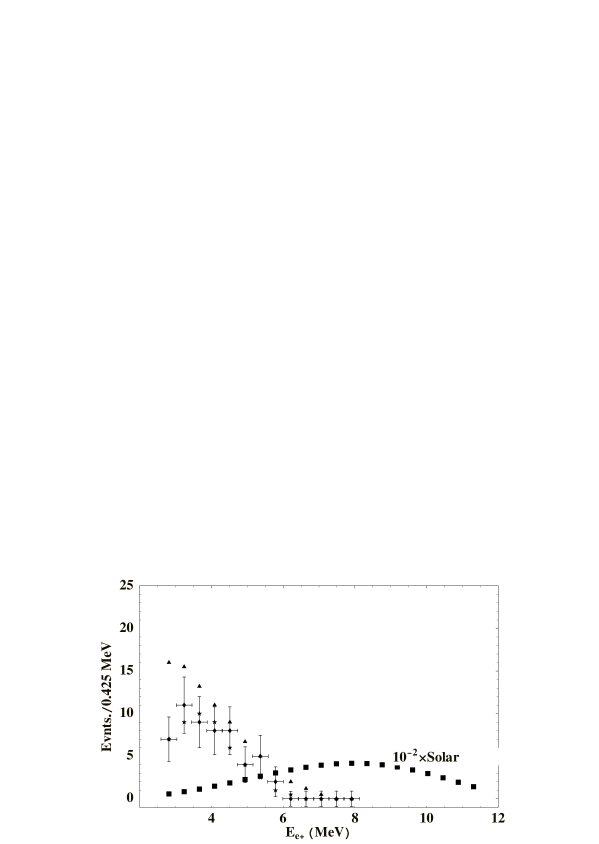
Figure 1: The KamLAND positron spectra from reactor antineutrinos (from Fig.5 in Ref.[1]): measured (145.5 days), MC expectations in absence of oscillations and best fit including neutrino oscillations ($\Delta m^{2}=6.9\times 10^{-5}$ eV², $\sin^{2}\theta=1$, respectively points with error-bars, triangles and stars). The “solar” positron spectrum (black solid squares) obtained assuming the shape of the ${}^{8}B$ neutrino flux and a total normalization $10^{-2}\times\Phi({}^{8}B)$ (that is, an overall $\nu_{e}-\overline{\nu}_{e}$ conversion probability $\overline{P}\sim 1\%$).

The results of our simulation are summarized in Fig.1 where we show the “solar” positron spectrum obtained assuming the shape of the ${}^{8}B$ neutrino flux and a total normalization $10^{-2}\times\Phi({}^{8}B)$ which means an overall $\nu_{e}-\overline{\nu}_{e}$ conversion probability $\overline{P}\sim 1\%$.

In addition we have computed the expected signal coming from antineutrino reactors. A number of short baseline experiments (See Ref.[21, vogel2] and references therein) have previously measured the energy spectrum of reactors at distances where oscillatory effects have been shown to be inexistent. They have shown that the theoretical neutrino flux predictions are reliable within 2% [22]. The effective flux of antineutrinos released by the nuclear plants is a rather well understood function of the thermal power of the reactor and the amount of thermal power emitted during the fission of a given nucleus, which gives the total amount, and the isotopic composition of the reactor fuel which gives the spectral shape. Detailed tables for these magnitudes can be found in Ref. [21, vogel2mq]. For a given isotope the energy spectrum can be parametrized by an exponential expression [18] where the coefficients depend on the nature of the fissionable isotope (see Ref.[21] for explicit values). Along the year, between periods of refueling, the total effective flux changes with time as the fuel is expended and the isotope relative composition varies. We take the average of the relative fission yields over the live time as given by the experiment: ${}^{235}U=57\%$, ${}^{238}U=7.8\%$, ${}^{239}Pu=30\%$, ${}^{241}Pu=5.7\%$. In order to obtain the expected number of events at KamLAND, we sum the expectations for all the relevant reactor sources weighting each source by its power and distance to the detector (table II in Ref. [21]), assuming the same spectrum originated from each reactor. We sum over the nearby power reactors, we neglect farther Japanese and Korean reactors and even farther rest-of-the-world reactors which give only a minor additional contribution.

3 Analysis and Results

We will obtain upper bounds on the solar electron antineutrino appearance probability analyzing the observed KamLAND rates in three different ways. In the first one, we will make a standard $\chi^{2}$ analysis of the observed and expected solar signals in the 13 prompt positron energy bins considered by KamLAND [1]. In the second and third cases we will apply Gaussian and poissonian probabilistic considerations to the global rate seen by the experiment and to the individual event content in the highest energy bins ($E_{e}>6$ MeV) where KamLAND observes zero events. This null signal makes particularly simple the extraction of statistical conclusions in this case.

3.1 Analysis of the KamLAND Energy Spectrum

Here we fully use the binned KamLAND signal (see Fig. 5 in Ref.[1]) for estimating the parameters of solar electron antineutrino production from the method of maximum-likelihood. We minimize the quantity

$$\chi^{2} = \chi^{2}_{i=1,9}+\chi^{2}_{i=10,13}$$ (3)

where the first term correspond to the contribution of the first nine bins where the signal is large enough and the use of the Gaussian approximation is justified. The second term correspond to the latest bins where the observed and expected signals are very small and poissonian statistics is needed. The explicit expressions are:

$$\chi^{2}_{i=1,9} = \sum_{i=1,9}\frac{(S_{i}^{exp}-S_{i}^{teo})^{2}}{\sigma^{2}}$$ (4)

$$\chi^{2}_{i=10,13} = 2\sum_{i=10,13}S_{i}^{teo}-S_{i}^{exp}+S_{i}^{exp}\log\frac{S_{i}^{exp}}{S_{i}^{teo}}.$$ (5)

The quantities $S_{i}$ are the observed bin contents from KamLAND. The theoretical signals are in principle a function of three different parameters: the solar electron antineutrino appearance probability $\overline{p}$ and the neutrino oscillation parameters $(\Delta m^{2},\theta)$. Both contributions, the contribution from solar antineutrinos and that one from solar reactors, can be treated as different summands:

$$S_{i}(\overline{p},\Delta m^{2},\theta) = S_{i}^{solar}(\overline{p})+S_{i}^{reactor}(\Delta m^{2},\theta).$$ (6)

According to our model, the solar antineutrino appearance probability $\overline{p}$ is taken as a constant and we can finally write:

$$S_{i}(\overline{p},\Delta m^{2},\theta) = \overline{p}\times S_{i}^{0}+S_{i}^{reactor}(\Delta m^{2},\theta).$$ (7)

In this work we will take for the minimization values of the oscillation parameters those obtained when ignoring any solar antineutrinos (LMA solution $\Delta m^{2}=6.9\times 10^{-5}$ eV², $\sin^{2}\theta=1$ from Ref.[1]) and we will perform a one-parameter minimization with respect $\overline{p}$. This approximation is well justified because the solar antineutrino probability is clearly very small, We avoid in this way the simultaneous minimization with respect to the three parameters ($\overline{p},\Delta m^{2},\theta)$.

We perform a minimization of the one dimensional function $\chi^{2}(\overline{p})$. to test a particular oscillation hypothesis against the parameters of the best fit and obtain the allowed interval in $\overline{p}$ parameter space taking into account the asymptotic properties of the likelihood function, i.e. $\log{\cal L}-\log{\cal L}_{min}$ behaves asymptotically as a $\chi^{2}$ with one degree of freedom. In our case, the minimization can be performed analytically because of the simple, lineal, dependence. A given point in the confidence interval is allowed if the globally subtracted quantity fulfills the condition $\Delta\chi^{2}=\chi^{2}(\overline{p})-\chi_{\rm min}^{2}<\chi^{2}_{n}(CL)$. Where $\chi^{2}_{n=1}(90\%,95\%,...)=2.70,3.84,..$ are the quantiles for one degree of freedom.

Restricting to physical values of $\overline{p}$, the minimum of the $\chi^{2}$ function is obtained for $\overline{p}=0$. The corresponding confidence intervals are $\overline{p}<4.5\%$ (90% CL) and $\overline{p}<7.0\%$ (95% CL). We have explicitly checked, varying the concrete place where the division between “Gaussian” and “poissonian” bins is established in Expression 3, that the values of these upper limits are largely insensitive to details of our analysis. In particular, similar upper limits are obtained in the extreme cases: if Gaussian or poissonian statistics is employed for all 13 bins. These upper limits are considerably weaker than those obtained in the next section. One possible reason for that is that they are obtained applying asymptotic general arguments to the $\chi^{2}$ distribution, stronger, or more precise limits could be obtained if a Monte Carlo simulation of the distribution of the finite sample $\chi^{2}$ distribution is performed (where the boundary condition $\overline{p}>0$ should be properly included).

3.2 Analysis of the global rate and highest energy bins

We can make an estimation of the upper bound on the appearance solar electron antineutrino probability simply counting the number of observed events and subtracting the number of events expected from the best-fit oscillation solution. For our purposes this difference, which in this case is positive, can be interpreted as a hypothetical signal coming from solar antineutrinos ($\Delta m^{2}_{0}=6.9\times 10^{5}\ eV^{2},\sin^{2}\theta_{0}=1)$.:

$$S_{solar}=\overline{p}\times S_{solar}^{0} = S_{obs}-S_{react}(\Delta m^{2}_{0},\sin^{2}\theta_{0}).$$ (8)

Putting [1] $S_{obs}=54.3\pm 7.5$ and $S_{react}(\Delta m^{2}_{0},\sin^{2}\theta_{0})=49\pm 1.3$, we obtain $S_{obs}-S_{react}<64.8\ (67.2)$ at 90 (95)% CL. From these numbers, the corresponding limits on solar electron antineutrino appearance probability are $\overline{p}<0.45\%,\ 0.52\%$ at 90 or 95% CL. These limits are valid for the neutrino energy range $E_{\nu}\sim 2-8$ MeV. In this case, due to the large range, the limits are better interpreted as limits on an energy-averaged probability according to expression 2.

In a similar approach, we use on continuation the binned KamLAND signal corresponding to the four highest energy bins (see Fig.1) which, as we will see, provide the strongest statistical significance and bounds. The reason for that is that the experiment KamLAND does not observe any signal here and, furthermore, the expected signal from oscillating neutrinos with LMA parameters is negligibly small.

Due to the small sample, we apply Poisson statistics to any of these bins and use the fact that a sum of Poisson variables of mean $\mu_{i}$ is itself a Poisson variable of mean $\sum\mu_{i}$. The background (here the reactor antineutrinos) and the signal (solar electron antineutrinos) are assumed to be independent Poisson Random variables with known means.

If no events are observed, and, in particular, no background is observed, the unified intervals [23, 17] $[0,\epsilon_{CL}]$ are $[0,2.44]$ at 90% CL and $[0,3.09]$ at 95% CL. From here, we obtain $\overline{p}\times S_{0}^{solar}<\epsilon_{CL}$ or $\overline{p}<\epsilon_{CL}/S_{0}^{solar}$. Taking the expected number of events in the first 145 days of data taking and in this energy range (6-8 MeV) we obtain: $\overline{p}<0.12\%$ (90% CL) and $\overline{p}<0.15\%$ (95% CL).

4 A model for solar antineutrino production

The combined action of spin flavor precession in a magnetic field and ordinary neutrino matter oscillations can produce an observable flux of $\overline{\nu}_{eR}$’s from the Sun in the case of the neutrino being a Majorana particle. In the simplest model, where a thin layer of highly chaotic of magnetic field is assumed at the bottom of the convective zone (situated at $R\sim 0.7R_{\odot}$), the antineutrino appearance probability at the exit of the layer $P(\overline{\nu})$ is basically equal to the appearance probability of antineutrinos at the earth [7, 6] ( see also Refs.[24] for some recent studies on RSFP solutions to the Solar Neutrino Problem). The quantity $P(\overline{\nu})$ is in general a function of the neutrino oscillation parameters $(\Delta m^{2},\theta)$, the neutrino intrinsic magnetic moment and also of the neutrino energy and the characteristics and magnitude of the solar magnetic field. However, in a accurate enough approximation, such probability can be factorized in a term depending only on the oscillation parameters and another one depending only on the spin-flavor precession parameters:

$$P(\overline{\nu})=\frac{1}{2}P_{e\mu}(\Delta m^{2},\theta)\times\left[1-\exp\left(-4\Omega^{2}\Delta r\right)\right]$$ (9)

where $P_{e\mu}$ is the $e-\mu$ solar conversion probability. We will assume in this work the LMA central values for $(\Delta m^{2},\theta)$ obtained from recent KamLAND data and which are compatible with the SNO observations in solar neutrinos [25], we will take $P_{e\mu}(\Delta m^{2},\theta)\simeq\langle P_{e\mu}\rangle^{exp,SNO}\simeq 0.4$. The second factor appearing in the expression contains the effect of the magnetic field. This quantity depends on the layer width $\Delta r$ ($\sim 0.1R_{\odot}$) and $\Omega^{2}\ \equiv\frac{1}{3}L_{0}\mu^{2}\langle B^{2}\rangle$, where $\langle B^{2}\rangle$ the r.m.s strength of the magnetic field and $L_{0}$ is a scale length ($L_{0}\sim 1000$ km). For small values of the argument we have the following approximate expression which is accurate enough for many applications

$$P(\overline{\nu})\simeq P_{e\mu}\times 2\Omega^{2}\Delta r=\kappa\ \mu^{2}\langle B^{2}\rangle$$

the solar astrophysical factor $\kappa\equiv 2/3P_{e\mu}L_{0}\Delta r$ is numerically $\kappa^{LMA}\simeq 2.8\times 10^{-44}$ MeV^-2. Upper limits on the antineutrino appearance probability can be translated into upper limits on the neutrino transition magnetic moment and the magnitude of the magnetic field in the solar interior. The results of the Formula 9 can be seen in Figure 2. An upper bound $\overline{p}<0.15-0.20\%$ (95% CL) implies an upper limit on the product of the intrinsic neutrino magnetic moment and the value of the convective solar magnetic field as $\mu B<2.3\times 10^{-21}$ MeV (95% CL). In Fig.2 we show the antineutrino probability as a function of the magnetic moment $\mu$ for fixed values of the magnitude of the magnetic field. For realistic values of other astrophysical solar parameters ($L_{0}\sim 1000$ km, $\Delta r\sim 0.1\ R_{\odot}$), these upper limits would imply that the neutrino magnetic moment is constrained to be, in the most desfavourable case, $\mu\mbox{$\leq$}3.9\times 10^{-12}\ \mu_{B}$ (95% CL) for a relatively small field $B=50$ kG. Stronger limits are obtained for slightly higher values of the magnetic field: $\mu\mbox{$\leq$}9.0\times 10^{-13}\ \mu_{B}$ (95% CL) for field $B=200$ kG and $\mu\mbox{$\leq$}2.0\times 10^{-13}\ \mu_{B}$ (95% CL) for field $B=1000$ kG. Let us note that these assumed values for the magnetic field at the base the solar convective zone are relatively mild and well within present astrophysical expectatives.

5 Conclusions

In summary in this work we investigate the possibility of detecting solar antineutrinos with the KamLAND experiment. These antineutrinos are predicted by spin-flavor solutions to the solar neutrino problem.

The KamLAND experiment is sensitive to potential antineutrinos originated from solar ⁸B neutrinos. We find that the results of the KamLAND experiment put relatively strict limits on the flux of solar electron antineutrinos $\Phi({}^{8}B)<1.1-3.5\times 10^{4}\ cm^{-2}\ s^{-1}$, and their energy averaged appearance probability ($P<0.15-0.50\%$). These limits are largely independent from any model on the solar magnetic field or any other astrophysical properties. As we remarked in Section 2.1, these upper limits on antineutrino probabilities and fluxes are still valid even if the antineutrino probabilities are significantly different from constant.

Next we assume a concrete model for antineutrino production where they are produced by spin-flavor precession in the convective solar magnetic field. In this model, the antineutrino appearance probability is given by a simple expression as $P(\overline{\nu})=\kappa\ \mu^{2}\langle B^{2}\rangle$ with $\kappa^{LMA}\simeq 2.8\times 10^{-44}$ MeV^-2. In the context of this model and assuming LMA central values for neutrino oscillation parameters ($\Delta m^{2}=6.9\times 10^{-5}$ eV², $\sin^{2}\theta=1$) [1], the upper bound $\overline{p}<0.15\%$ (95% CL) implies an upper limit on the product of the intrinsic neutrino magnetic moment and the value of the convective solar magnetic field as $\mu\ B<2.3\times 10^{-21}$ MeV (95% CL). For realistic values of other astrophysical solar parameters these upper limits would imply that the neutrino magnetic moment is constrained to be, in the most desfavourable case, $\mu\mbox{$\leq$}3.9\times 10^{-12}\ \mu_{B}$ (95% CL) for a relatively small field $B=50$ kG. For slightly higher values of the magnetic field: $\mu\mbox{$\leq$}9.0\times 10^{-13}\ \mu_{B}$ (95% CL) for field $B=200$ kG and $\mu\mbox{$\leq$}2.0\times 10^{-13}\ \mu_{B}$ (95% CL) for field $B=1000$ kG. These assumed values for the magnetic field at the base the solar convective zone are relatively mild and well within present astrophysical expectatives.

Acknowledgments

I would like to acknowledge many useful conversations with P. Aliani, M. Picariello and V. Antonelli. I acknowledge the financial support of the Spanish CYCIT funding agency.

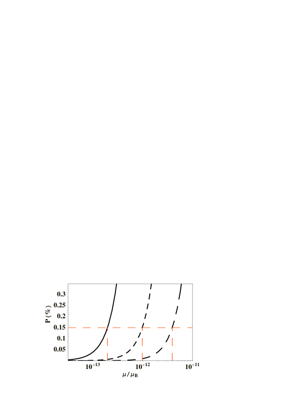
Figure 2: The solar antineutrino appearance probability $\overline{p}$ as a function of the transition neutrino magnetic moment, in units of Bohr magnetons $\mu_{B}$, for fixed values of the r.m.s solar magnetic field (Formula 9). From left (solid) to right (dashed), curves correspond to $B=1000,200,50$ kG. From the curves, an upper limit $\overline{p}<0.15\%$ implies $\mu<1.9\times 10^{-13}\mu_{B},9.0\times 10^{-13}\mu_{B},3.0\times 10^{-12}\mu_{B}$ respectively for each of the magnetic field above.

References

- [1] K. Eguchi et al. [Kamland Collaboration], arXiv:hep-ex/0212021.
- [2] J. N. Bahcall, M. C. Gonzalez-Garcia and C. Pena-Garay, arXiv:hep-ph/0212147. A. Bandyopadhyay, S. Choubey, R. Gandhi, S. Goswami and D. P. Roy, arXiv:hep-ph/0212146. W. l. Guo and Z. z. Xing, arXiv:hep-ph/0212142. M. Maltoni, T. Schwetz and J. W. Valle, arXiv:hep-ph/0212129. G. L. Fogli, E. Lisi, A. Marrone, D. Montanino, A. Palazzo and A. M. Rotunno, arXiv:hep-ph/0212127. V. Barger and D. Marfatia, arXiv:hep-ph/0212126. G. Barenboim, L. Borissov and J. Lykken, arXiv:hep-ph/0212116.
- [3] M. Apollonio et al. (CHOOZ coll.), hep-ex/9907037, Phys. Lett. B 466 (1999) 415. M. Apollonio et al., Phys. Lett. B 420 (1998) 397. F. Boehm et al.,Phys. Rev. D62 (2000) 072002 [hep-ex/0003022].
- [4] Y. F. Wang [Palo Verde Collaboration], Int. J. Mod. Phys. A 16S1B, 739 (2001); F. Boehm et al., Phys. Rev. D 64, 112001 (2001).
- [5] P. Aliani, V. Antonelli, M. Picariello and E. Torrente-Lujan, JHEP 0302:025,2003.
- [6] E. Torrente-Lujan, Prepared for 2nd ICRA Network Workshop: The Chaotic Universe: Theory, Observations, Computer Experiments, Rome, Italy, 1-5 Feb 1999. E. Torrente-Lujan, arXiv:hep-ph/9912225. E. Torrente-Lujan, Phys. Rev. D 59, 093006 (1999). E. Torrente-Lujan, Phys. Rev. D 59, 073001 (1999). E. Torrente-Lujan, arXiv:hep-ph/9602398. V. B. Semikoz and E. Torrente-Lujan, Nucl. Phys. B 556, 353 (1999). E. Torrente-Lujan, arXiv:hep-ph/0210037. E. Torrente Lujan, Phys. Rev. D 53, 4030 (1996).
- [7] E. Torrente-Lujan, Phys. Lett. B 441, 305 (1998).
- [8] J. N. Bahcall, M. H. Pinsonneault and S. Basu, Astrophys. J. 555, 990 (2001).
- [9] Q. R. Ahmad et al. [SNO Collaboration], Phys. Rev. Lett. 89, 011301 (2002).
- [10] Q. R. Ahmad et al. [SNO Collaboration], Phys. Rev. Lett. 89, 011302 (2002).
- [11] P. Aliani, V. Antonelli, R. Ferrari, M. Picariello and E. Torrente-Lujan, Phys. Rev. D 67 (2003) 013006.
- [12] A. Strumia, C. Cattadori, N. Ferrari and F. Vissani, arXiv:hep-ph/0205261. A. Bandyopadhyay, S. Choubey, S. Goswami and D. P. Roy, Phys. Lett. B 540, 14 (2002). V. Barger, D. Marfatia, K. Whisnant and B. P. Wood, Phys. Lett. B 537, 179 (2002). J. N. Bahcall, M. C. Gonzalez-Garcia and C. Pena-Garay, arXiv:hep-ph/0204314. S. Pascoli and S. T. Petcov, arXiv:hep-ph/0205022. P. C. de Holanda and A. Y. Smirnov, arXiv:hep-ph/0205241. R. Foot and R. R. Volkas, arXiv:hep-ph/0204265.
- [13] P. Aliani, V. Antonelli, R. Ferrari, M. Picariello and E. Torrente-Lujan, arXiv:hep-ph/0206308. S. Khalil and E. Torrente-Lujan, J. Egyptian Math. Soc. 9, 91 (2001) [arXiv:hep-ph/0012203]. E. Torrente-Lujan, arXiv:hep-ph/9902339.
- [14] P. Aliani, V. Antonelli, M. Picariello and E. Torrente-Lujan, Nucl. Phys. B634 (2002) 393-409. P. Aliani, V. Antonelli, M. Picariello and E. Torrente-Lujan, Nucl. Phys. Proc. Suppl. 110, 361 (2002) [arXiv:hep-ph/0112101]. P. Aliani, V. Antonelli, R. Ferrari, M. Picariello and E. Torrente-Lujan, arXiv:hep-ph/0205061.
- [15] V. Barger, D. Marfatia and K. Whisnant, arXiv:hep-ph/0106207.
- [16] E. Torrente-Lujan, Nucl. Phys. Proc. Suppl. 87, 504 (2000). E. Torrente-Lujan, Phys. Lett. B 494, 255 (2000).
- [17] “Review of Particle Properties”, K. Hagiwara et al. (Particle Data Group), Phys. Rev. D 66 (2002) 010001
- [18] P. Vogel and J. F. Beacom, Phys. Rev. D 60, 053003 (1999).
- [19] P. Aliani, V. Antonelli, M. Picariello and E. Torrente-Lujan, New J. Phys. 5 (2003) 2. P. Aliani, V. Antonelli, R. Ferrari, M. Picariello and E. Torrente-Lujan, arXiv:hep-ph/0211062. P. Aliani, V. Antonelli, M. Picariello and E. Torrente-Lujan, arXiv:hep-ph/0208089.
- [20] G.Horton-Smith, Neutrinos and Implications for Physics Beyond the Standard Model, Stony Brook, Oct. 11-13, 2002. http://insti.physics.sunysb.edu/itp/conf/neutrino.html A.Suzuki. Texas in Tuscany, XXI Symposium on Relativistic Astrophysics Florence, Italy, December 9-13, 2002. http://www.arcetri.astro.it/ texaflor/.
- [21] H. Murayama and A. Pierce, Phys. Rev. D 65 (2002) 013012. [vogel2] P. Vogel, A. Engel, Phys. Rev. D39, 3378 (1989).
- [22] A. Piepke [Kamland collaboration], Nucl. Phys. Proc. Suppl. 91, 99 (2001)
- [23] G. J. Feldman and R. D. Cousins, Phys. Rev. D 57, 3873 (1998).
- [24] E. K. Akhmedov, arXiv:hep-ph/0207342. E. K. Akhmedov and J. Pulido, Phys. Lett. B 553, 7 (2003). E. K. Akhmedov and J. Pulido, Phys. Lett. B 553, 7 (2003). B. C. Chauhan, arXiv:hep-ph/0204160. B. C. Chauhan, S. Dev and U. C. Pandey, Phys. Rev. D 59, 083002 (1999) [Erratum-ibid. D 60, 109901 (1999)]. U. C. Pandey, B. C. Chauhan and S. Dev, Mod. Phys. Lett. A 13, 3201 (1998). B. C. Chauhan and J. Pulido, Phys. Rev. D 66, 053006 (2002). E. K. Akhmedov and J. Pulido, Phys. Lett. B 529, 193 (2002). J. Pulido, Astropart. Phys. 18, 173 (2002). E. K. Akhmedov and J. Pulido, Phys. Lett. B 485, 178 (2000). J. Pulido and E. K. Akhmedov, Astropart. Phys. 13, 227 (2000).
- [25] P. Aliani, V. Antonelli, M. Picariello and E. Torrente-Lujan, arXiv:hep-ph/0212212.