We investigate the deeply virtual Compton scattering (DVCS) in the color dipole approach, implementing the dipole cross section through the saturation model, which interpolates successfully between soft and hard regimes. The imaginary and real part of the DVCS amplitude are obtained and the results are compared to the available data.

 

1 Introduction

The investigation of hard exclusive reactions in the Bjorken limit is a reliable acces of obtaining information into details on the structure of the nucleon which could not be obtained considering inclusive deep inelastic processes. The probe provided by the photon works as a clean tool reactions in order to extract reliable knowledge on the substructure of strongly interacting particles complementar to exclusive vector meson production [1]. The recent data from the DESY $ep$ collider HERA on exclusive diffractive virtual Compton process [2, 3] (DVCS) at large $Q^{2}$ becomes an important source to study the partons, in particular gluons, inside the proton for nonforward kinematics and its relation with the forward one. These features are encoded in the formalism of the so-called skewed parton distributions, where dynamical correlations between partons with different momenta are taken into account. A considerable interest of the DVCS process lies in the particular access it gives to these generalized parton distributions (GDP) through the interference term with the Bethe-Heitler process. The high energy situation at HERA gives the important opportunity to constrain the gluon contribution to GPDs and to study the evolution in virtuality $Q^{2}$ of the quark and gluon distributions. On the other hand, recently the color dipole formalism has provided a simultaneous description of photon induced process. The inclusive deep inelastic reaction and the photon diffractive dissociation has been successfully described and the study of other exclusive processes such as DVCS is an important test of the color dipole approach.

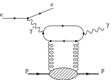
Figure 1: The two leading DVCS QCD diagrams. The LO diagram in the QCD picture on the left graph and the NLO diagram on the right.

The color dipole model of diffraction is a simple unified picture of diffractive processes which provides a large phenomenology on the Deep Inelastic Scattering (DIS) regime. In the proton rest frame, the DVCS process can be seen as a succession in time of three factorisable subprocesses: i) the photon fluctuates in a quark-antiquark pair, ii) this coulour dipole interacts with the proton target, iii) the quark pair annihilates in a real photon. Using as kinematic variables the $\gamma^{*}p$ c.m.s. energy squared $s=W^{2}=(p+q)^{2}$, where $p$ and $q$ are the proton and the photon momenta respectively, the photon virtuality squared $Q^{2}=-q^{2}$ and the Bjorken scale $x=Q^{2}/(W^{2}+Q^{2})$, the corresponding amplitude at zero momentum transfer reads as,

$${\cal I}m\,{\cal A}_{T,L}(s,Q^{2},\,t=0) = \sigma^{\gamma^{*}p}_{T,\,L}(x,\,Q^{2})=\int_{0}^{1}dz\,\int d^{2}\mbox{\boldmath$r$}\,|\Psi_{T,\,L}(z,\,\mbox{\boldmath$r$},\,Q^{2})|^{2}\,\sigma_{dip}(\tilde{x},\,\mbox{\boldmath$r$}^{2})\,,$$ (1)

$$|\Psi_{T}(z,\mbox{\boldmath$r$},\,Q^{2})|^{2} = \frac{6\alpha_{\mathrm{em}}}{4\,\pi^{2}}\,\sum_{f}e_{f}^{2}\,\left\{[z^{2}+(1-z)^{2}]\,\varepsilon^{2}\,K_{1}^{2}(\varepsilon\,\mbox{$r$})+m_{f}^{2}\,\,K_{0}^{2}(\varepsilon\,\mbox{$r$})\right\}\,,$$ (2)

$$|\Psi_{L}(z,\mbox{\boldmath$r$},\,Q^{2})|^{2} = \frac{6\alpha_{\mathrm{em}}}{\pi^{2}}\,\sum_{f}e_{f}^{2}\,\left\{Q^{2}\,z^{2}(1-z)^{2}\,K_{0}^{2}(\varepsilon\,\mbox{$r$})\right\}\,,$$ (3)

where $\Psi_{T,\,L}$ are the photon wave function for transverse ($T$) and longitudinal ($L$) photons, respectively. They are well known from usual QED coupling, where $r$ defines the relative transverse separation of the pair (dipole) and $z$, $(1-z)$, are the longitudinal momentum fractions of the quark (antiquark). The auxiliary variable $\varepsilon^{2}=z(1-z)\,Q^{2}+m^{2}_{f}$ depends on the quark mass, $m_{f}$. The $K_{0,1}$ are the McDonald functions and summation is performed over the quark flavors.

The dipole cross section $\sigma_{dip}$ describing the dipole-proton interaction is substantially affected by non-perturbative content. There are several phenomenological implementations for this quantity. The main feature in a successful model is to be able to match the soft (low $Q^{2}$) and hard (large $Q^{2}$) regimes in a unified way. This has been achieved in models using Regge approach [4], QCD color transparency phenomena [5] and/or hybrid ones mixing non-perturbative functional approach and Regge phenomenology [6]. Phenomenological analysis including a parton saturation phenomenon at high energies has been considered, for instance in [7, 8].

In the present work we follow the quite successful saturation model [9], which interpolates between the small and large dipole configurations, providing color transparency behavior, $\sigma_{dip}\sim\mbox{\boldmath$r$}^{2}$, as $\mbox{\boldmath$r$}\rightarrow 0$ and constant behavior, $\sigma_{dip}\sim\sigma_{0}$, at large dipoles. The parameters of the model have been obtained from an adjustment to small $x$ HERA data. Its free-parameter application to diffractive DIS has been also quite successful [10]. The parametrisation for the dipole cross section takes the eikonal-like form,

$$\sigma_{dip}(\tilde{x},\,\mbox{\boldmath$r$}^{2}) = \sigma_{0}\,\left[\,1-\exp\left(-\frac{\,Q_{s}^{2}(x)\,\mbox{\boldmath$r$}^{2}}{4}\right)\,\right]\,,$$ (4)

$$Q_{s}^{2}(x) = \left(\frac{x_{0}}{\tilde{x}}\right)^{\lambda}\,\,\mathrm{GeV}^{2}\,,$$ (5)

where the saturation scale $Q_{s}^{2}$ defines the onset of the saturation phenomenon, which depends on energy. The parameters were obtained from a fit to the HERA data producing $\sigma_{0}=23.03\,(29.12)$ mb, $\lambda=0.288\,(0.277)$ and $x_{0}=3.04\cdot 10^{-4}\,(0.41\cdot 10^{-4})$ for a 3-flavor (4-flavor) analysis [9]. An additional parameter is the effective light quark mass, $m_{f}=0.14$ GeV. It is worth to mention that the quark mass plays the role of a regulator for the photoproduction ($Q^{2}=0$) cross section. The charm quark mass is considered to be $m_{c}=1.5$ GeV. A smooth transition to the photoproduction limit is obtained with a modification of the Bjorken variable as,

$$\tilde{x}=x\,\left(\,1+\frac{4\,m_{f}^{2}}{Q^{2}}\,\right)\,.$$ (6)

Recently, a new implementation of the model including QCD evolution [11] (labeled in the following BGK model) has appeared. It will be considered in the calculation to be presented in the last section. Now, the dipole cross section depends on the gluon distribution in the following way,

$$\sigma_{dip}(\tilde{x},\,\mbox{\boldmath$r$}^{2}) = \sigma_{0}\,\left[\,1-\exp\left(-\frac{\,\pi^{2}\,\mbox{\boldmath$r$}^{2}\,\alpha_{s}(\mu^{2})\,\tilde{x}\,G(\tilde{x},\mu^{2})}{3\,\sigma_{0}}\right)\,\right]\,,$$ (7)

$$x\,G(x,\mu^{2}) = A_{g}\,x^{-\lambda_{g}}\,(1-x)^{5.6}\,,$$ (8)

where $\mu^{2}=C/\mbox{\boldmath$r$}^{2}+\mu_{0}^{2}$. The parameters ($C$ and $\mu_{0}^{2}$) are determined from a fit to DIS data. The flavor number is taken to be equal to 3. The overall normalization $\sigma_{0}=23.03$ mb is kept fixed (labeled fit 1 in Ref. [11]). The function $G(x,\mu^{2})$ is evolved with the leading order DGLAP evolution equation for the gluon density with initial scale $Q_{0}^{2}=1$ GeV². The improvement preserves the main features of the low-$Q^{2}$ and transition regions, while providing QCD evolution in the large-$Q^{2}$ domain.

In this paper we test the validity of the saturation model in the particular case of the DVCS: $\gamma^{*}p\rightarrow\gamma p$, where the final photon is real. The DVCS consists in the simplest exclusive diffractive process as it does not imply uncertainties due to the composite meson wave function in the final state like in the vector meson production, $\gamma^{*}p\rightarrow Vp$. On the other hand, as we will see, the restriction to the transverse part of the photon wave function (at the leading twist), due to the real photon, enhances the contribution of larger dipole configurations and therefore the sensitivity, w.r.t the inclusive DIS case, to the soft content of the proton and the transition between the hard and soft regimes. This is why we believe that the DVCS process provides a particularly relevant test, in a parameter free way, of the saturation model. The recent cross section measurements from H1 [2] and ZEUS [3] at HERA allow us now to confront the saturation model prediction.

The paper is organized as follows. In the next section we address the main formulae of the DVCS process in the color dipole picture applying the dipole cross section given by the saturation model in order to investigate and to calculate the imaginary and real part of the referred amplitude. In the last section we compare the results obtained with the DVCS measurement of the H1 Collaboration, taking into account the three(four)-flavor analysis model. The results obtained using the recent QCD improvement to the original model are also presented. There, we discuss the different characteristics coming from the distinct analysis and present a qualitative study of the DVCS cross section using the saturation model.

2 Deeply virtual Compton scattering in the color dipole picture

In this section we establish the deeply virtual Compton scattering amplitude and the profile function expressions.

Applying the color dipole approach to the DVCS process, the imaginary part of the amplitude at zero momentum transfer reads as,

$${\cal I}m\,{\cal A}\,(s,Q^{2},t=0)=\int_{0}^{1}dz\,\int d^{2}\mbox{\boldmath$r$}\,\Phi_{T}(z,\,\mbox{\boldmath$r$},\,Q^{2})\,\sigma_{dip}(\tilde{x},\,\mbox{\boldmath$r$}^{2})\,,$$ (9)

$$\Phi_{T}(z,\,\mbox{\boldmath$r$},\,Q^{2})\equiv\Psi_{T}^{*}(z,\,\mbox{\boldmath$r$},\,Q_{1}^{2}=Q^{2})\,\Psi_{T}(z,\,\mbox{\boldmath$r$},\,Q_{2}^{2}=0)\,,$$ (10)

$$\Phi_{T}=\frac{6\alpha_{\mathrm{em}}}{4\,\pi^{2}}\,\sum_{f}e_{f}^{2}\,\left\{[z^{2}+(1-z)^{2}]\,\varepsilon_{1}\,K_{1}(\varepsilon_{1}\,\mbox{$r$})\,\varepsilon_{2}\,K_{1}(\varepsilon_{2}\,\mbox{$r$})+m_{f}^{2}\,\,K_{0}(\varepsilon_{1}\,\mbox{$r$})\,K_{0}(\varepsilon_{2}\,\mbox{$r$})\right\}\,,$$ (11)

where $\varepsilon^{2}_{1,\,2}=z(1-z)\,Q_{1,\,2}^{2}+m_{f}^{2}$.

The relative contributions from dipoles of different sizes can be analyzed with the weight (profile) function,

$$W(\mbox{\boldmath$r$},Q^{2})=\int_{0}^{1}\,dz\;r\;\Phi_{T}(z,\mbox{\boldmath$r$},Q^{2})\;\sigma_{dip}\,(\tilde{x},\,\mbox{\boldmath$r$}^{2})\,.$$ (12)

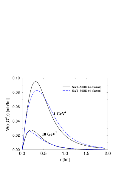
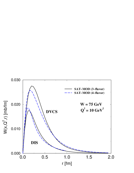
Figure 2: (a) The weight function $W(\mbox{\boldmath$r$},Q^{2})$ as a function of the dipole size $r$ at fixed c.m.s energy $W=75$ GeV for two virtualities: $Q^{2}=1$ GeV² and $Q^{2}=10$ GeV². The solid lines correspond to a 3-flavor analysis whereas the long-dashed ones are for the 4-flavor case. (b) Comparison between the profile function for DVCS and inclusive DIS processes at $Q^{2}=10$ GeV², using the same notation.

In Fig. (2-a), the weight function $W(\mbox{\boldmath$r$},Q^{2})$ is shown as a function of the dipole size $r$ at fixed c.m.s energy $W=75$ GeV and at two virtualities. The dipole cross section is taken from Eq. (4). We analyze the $r$-profile for a low virtuality $Q^{2}=1$ GeV² and for a large one, $Q^{2}=10$ GeV². Our conclusions are similar to those in Ref. [12], i.e. as the virtualities increase the contribution of large dipole configurations diminishes in a sizable way. The calculation was performed using both a 3-flavor and a 4-flavor analysis. The inclusion of the charm content gives a slightly lower normalization for the profile and by consequence for the total cross section. It is worth to mention that the situation is different in the inclusive DIS case, where the transverse wave function is symmetric on $\varepsilon_{1,2}$ [for instance, see Eqs. (2) and (11)] and the results including charm slightly differ from those using only light quarks. This is shown in Fig. (2-b) where one compares the DVCS and inclusive DIS profiles at $Q^{2}=10$ GeV² using light quarks and adding charm contribution. The impact of charm is smaller in the inclusive DIS case than in the DVCS process. Furthermore, it is verified that the DVCS profile selects larger dipole sizes in contrast to the inclusive DIS profile, even in the analysis including charm. Therefore, DVCS is more sensitive to the non-perturbative (soft) content of the scattering process.

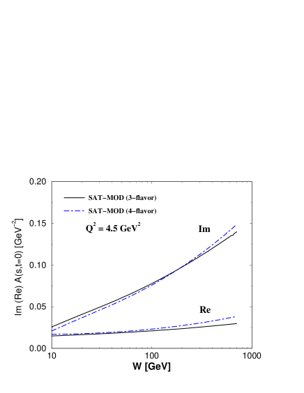
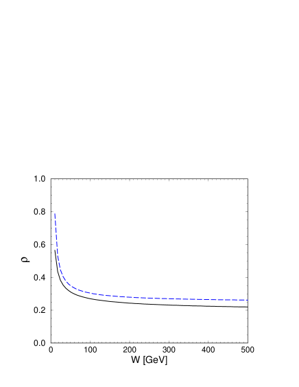
Figure 3: (a) The imaginary and real part of the DVCS amplitude as a function of the c.m.s. energy $W$ at $Q^{2}=4.5$ GeV². (b) The ratio real to imaginary part, the parameter $\rho$ as a function of $W$ at $Q^{2}=4.5$ GeV². The solid lines correspond to the 3-flavor analysis and the long-dashed ones to the 4-flavor analysis.

In order to compute the real part of the DVCS amplitude in the approach above, we have considered the dispersion relations as done in of Ref. [12]. In Fig. (3-a) both the imaginary and real part of the amplitude using the saturation model are shown as a function of c.m.s. energy $W$ at $Q^{2}=4.5$ GeV². The ratio of the real to imaginary part, the $\rho$ parameter, is presented in the Fig. (3-b). The analysis was done considering the light quarks (the solid lines) and also including the charm content (the long-dashed lines). The latter gives a lower overall normalization for the amplitudes, as referred before. The procedure in order to obtain the real part of amplitude and the $\rho$ parameter was taken from Ref. [13], where a two-power adjustment to the imaginary part of the amplitude is made,

$${\cal I}m\,{\cal A}\,(s,t=0)=A_{1}\,\left(\frac{W^{2}}{W_{0}^{2}}\right)^{\lambda_{1}}+A_{2}\,\left(\frac{W^{2}}{W_{0}^{2}}\right)^{\lambda_{2}}\,,$$ (13)

and the real part and $\rho$ are given by,

$${\cal R}e\,{\cal A}\,(s,t=0) = A_{1}\,\left(\frac{W^{2}}{W_{0}^{2}}\right)^{\lambda_{1}}\,\tan\left(\frac{\pi\,\lambda_{1}}{2}\right)+A_{2}\,\left(\frac{W^{2}}{W_{0}^{2}}\right)^{\lambda_{2}}\tan\left(\frac{\pi\,\lambda_{1}}{2}\right)\,,$$ (14)

$$\rho = \frac{\tan(\pi\,\lambda_{1}/2)+A_{2}/A_{1}\,(W^{2}/W_{0}^{2})^{\lambda_{2}-\lambda_{1}}\,\tan(\pi\,\lambda_{2}/2)}{1+A_{2}/A_{1}\,(W^{2}/W_{0}^{2})^{\lambda_{2}-\lambda_{1}}}\,.$$ (15)

The parameters obtained from a 3-flavor (4-flavor) analysis are presented in Table (1). The effect in the DVCS total cross section is of order 12 % in the overall normalisation at $W=75$ GeV ($\rho\approx 0.35$). From Fig. (3-b), the $\rho$ parameter depends weakly on $W$ for $W\geq 100$ GeV, tending asymptotically to $\rho\approx 0.3$.

Parameter	(3-flavor)	(4-flavor)
$A_{1}$	-0.056	-0.0336373
$A_{2}$	0.0368	0.0285722
$\lambda_{1}$	-0.060	-0.202454
$\lambda_{2}$	0.1059	0.152216
$W_{0}^{2}$	0.3746	8.28475

Table 1: Parameters of the two-power adjustment to the imaginary part of the amplitude, with a 3-flavor (4-flavor) analysis.

Finaly, we calculate the ratio between the imaginary parts of the forward $t=0$ amplitudes for DIS and DVCS, $\mathrm{R}={\cal I}m\,\,\mathrm{DIS}/\,{\cal I}m\,\,\mathrm{DVCS}$. This quantity is quite interesting as it shows the importance of the skewing effect. In Fig. (4) are shown the results obtained from the 3-flavor (solid line) and 4-flavor (dashed line) analysis of the saturation model at fixed $W=75$ GeV as a function of the virtuality $Q^{2}$. The obtained values are slightly above those from an aligned jet model analysis in Ref. [14] and below those from the dipole analysis in Ref. [12].

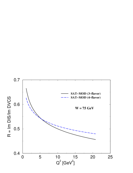
Figure 4: The ratio of the imaginary parts of the DIS and DVCS amplitudes as a function of $Q^{2}$ at fixed $W=75$ GeV. The solid lines correspond to the 3-flavor analysis and the long-dashed ones to the 4-flavor analysis.

3 Results and conclusions

We are able now to compare our results with the H1 Collaboration DVCS measurement at the photon level [2]. The final expression for the DVCS cross section is written as,

$$\sigma(\gamma^{*}\,p\rightarrow\gamma\,p) = \frac{1}{B}\,\left.\frac{d\sigma}{dt}\right|_{t=0}\,,$$ (16)

$$\left.\frac{d\sigma}{dt}\right|_{t=0} = \frac{[\,{\cal I}m\,{\cal A}(s,0)\,]^{2}}{16\,\pi}\,(1+\rho^{2})\,,$$ (17)

where $B$ is the $t$ slope parameter and comes from a simple exponential parametrisation and the $\rho$ parameter has been determined in the previous section. The $B$ value has never been measured for DVCS. The H1 publication compares its cross section measurement to several predictions for $5<B<9$ GeV^-2 [2]. As a first calculation, we present the results considering the saturation model for the 3-flavor analysis. The plots present an upper (lower) value corresponding to the slope values $B=5$ GeV^-2 ($B=9$ GeV^-2). In Fig. (5-a) the DVCS cross section is shown as a function of $W$ at fixed $Q^{2}=4.5$ GeV² and in Fig. (5-b) as a function of $Q^{2}$ at fixed $W=75$ GeV. We have verified that the inclusion of charm produces a normalization slightly lower than using only the light quarks where one considers the same $B$ value. This feature is more pronounced in the cross section as a function of energy, whereas is less significant in the $Q^{2}$ behaviour. Concerning the choice of the quark mass values it should be noted that, taking $m_{f}=0$ increases the cross sections for the 3-flavor (4-flavor) analysis by a factor 1.15 (1.17) at $W$=20 GeV down to 1.13 (1.16) at $W$=120 GeV at the average $Q^{2}=4.5$ GeV². This factor increases slightly for lower $Q^{2}$ values. Keeping $m_{f}$ fixed enhances the overall normalization for lower $m_{c}$, as usual.

As a second calculation, we present the results considering the saturation model for the 4-flavor analysis. The plots present an upper (lower) value corresponding to the slope values $B=5$ GeV^-2 ($B=9$ GeV^-2). In the Fig. (6-a) the DVCS cross section is shown as a function of $W$ at fixed $Q^{2}=4.5$ GeV² and in Fig. (6-b) as a function of $Q^{2}$ at fixed $W=75$ GeV. The conclusions are similar as in the 3-flavor case.

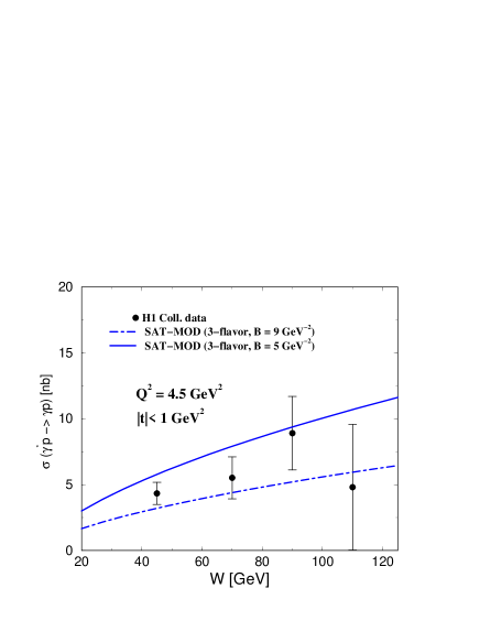
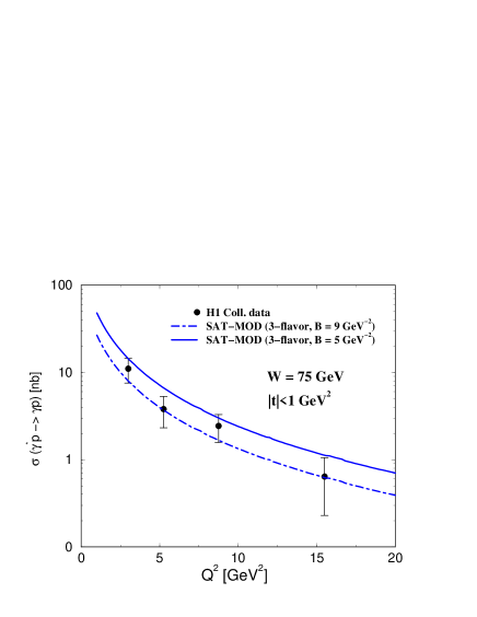
Figure 5: (a) Saturation model: a 3-flavor analysis. The photon level DVCS cross section as a function of the c.m.s. energy $W$ at $Q^{2}=4.5$ GeV² considering the band for the slope $5<B<9$ GeV^-2 . (b) The DVCS cross section as a function of the virtuality $Q^{2}$ at fixed $W=75$ GeV, considering the same notation.

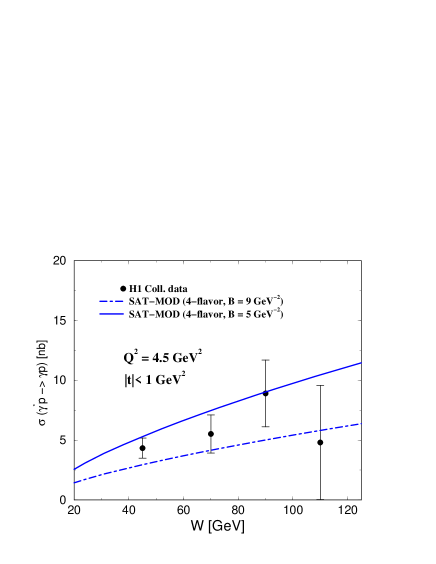
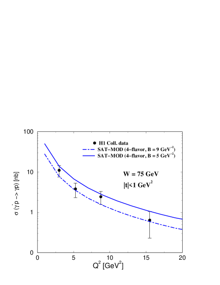
Figure 6: (a) Saturation model: a 4-flavor analysis. The photon level DVCS cross section as a function of the c.m.s. energy $W$ at $Q^{2}=4.5$ GeV² considering the band for the slope $5<B<9$ GeV^-2 . (b) The DVCS cross section as a function of the virtuality $Q^{2}$ at fixed $W=75$ GeV, using the same notation.

In what follows, due to the absence of a consistent constraint on the normalization, we will use the $B$ value which fits the best with the H1 measurement for each prediction. In Fig. (7) the following calculations are presented: (i) the saturation model for a 3-flavor analysis (solid line); (ii) the saturation model for a 4-flavor analysis (dashed line) ; (iii) the QCD improved saturation model (dot-dashed line), given by Eq. (8). The corresponding slope values are shown in the plot. We have not included the real part of the amplitude for the BGK case. The present result shows how important it is to measure the $B$ slope in order to discriminate among the available approaches. It should be stressed that the result from the BGK model deserves more studies, since a 4-flavor analysis was not done yet and skewed effects needed in DVCS are not available in this model.

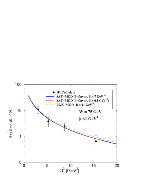
Figure 7: (a) The photon level DVCS cross section as a function of virtuality $Q^{2}$ at fixed $W=75$ GeV. The plots correspond to the 3-flavor and 4-flavor analysis of the saturation model (solid and dashed lines) and the BGK model (dot-dashed line). The corresponding $B$ slopes are also presented.

It is timely to perform a qualitative analysis in order to obtain a clear physical interpretation using the saturation model, as done for the DIS case in [9]. In the following we should consider for simplicity the particular case $m_{f}=0$. The imaginary part of the DVCS amplitude is given by the integrations over the dipole size $r$ and longitudinal momentum fraction $z$ in Eq. (9). One can use the small approximation argument for the Bessel function $K_{1}(x)$, such that $K_{1}(x)=1/x$ for $x\ll 1$ and is exponentially suppressed for $x\gg 1$. Then, we can write:

$${\cal I}m\,{\cal A}\,(s,t=0)\sim\int_{0}^{4/Q^{2}}\frac{d\mbox{$r$}^{2}}{\mbox{$r$}^{2}}\,\sigma_{dip}\,(\tilde{x},\,\mbox{\boldmath$r$}^{2})+\int_{4/Q^{2}}^{\infty}\frac{d\mbox{$r$}^{2}}{\mbox{$r$}^{2}}\,\left(\frac{1}{Q^{2}\,\mbox{$r$}^{2}}\right)\sigma_{dip}\,(\tilde{x},\,\mbox{\boldmath$r$}^{2})$$ (18)

where the first term is domainated by symmetric contributions, i.e. the quark and the antiquark constituting the dipole share almost the same momentum fraction $z$ and the distribution on that variable is uniform around the mean value $z=1/2$. The second term is domainated by aligned jet or asymmetric configurations, where $z$ or $(1-z)$ takes a vanishing value and the $z$ integration is restricted to $z\raisebox{-1.42262pt}{$\stackrel{{\scriptstyle<}}{{\scriptstyle{\sim}}}$}1/(Q^{2}\,\mbox{$r$}^{2})$.

In order to proceed in the qualitative analysis, one can use an approximate form for the dipole cross section from the saturation model; $\sigma_{dip}=\sigma_{0}\,\mbox{$r$}^{2}\,Q_{s}^{2}/4$ for $\mbox{$r$}^{2}\leq 4/Q_{s}^{2}$ and $\sigma_{dip}=\sigma_{0}$ for $\mbox{$r$}^{2}>4/Q_{s}^{2}$. The saturation scale is given by $Q_{s}^{2}(x)=1/R_{0}^{2}\simeq x^{-\lambda}$. Therefore, if the typical dipole size, $1/Q$, is much smaller than the mean distance between partons $R_{0}^{2}(x)$, the expression for the amplitude becomes,

$${\cal I}m\,{\cal A}\,(s,t=0) \sim \int_{0}^{4/Q^{2}}\frac{d\mbox{$r$}^{2}}{\mbox{$r$}^{2}}\,\left(\frac{\sigma_{0}\,\mbox{$r$}^{2}\,Q_{s}^{2}(x)}{4}\right)+\int_{4/Q^{2}}^{4/Q_{s}^{2}(x)}\frac{d\mbox{$r$}^{2}}{\mbox{$r$}^{2}}\,\left(\frac{1}{Q^{2}\,\mbox{$r$}^{2}}\right)\,\left(\frac{\sigma_{0}\,\mbox{$r$}^{2}\,Q_{s}^{2}(x)}{4}\right)$$ (19)

$$+\int_{4/Q_{s}^{2}(x)}^{\infty}\frac{d\mbox{$r$}^{2}}{\mbox{$r$}^{2}}\,\left(\frac{1}{Q^{2}\,\mbox{$r$}^{2}}\right)\,\sigma_{0}\,,$$

where the first term comes from symmetric configurations and the remaining ones from the asymmetric configurations. The final result in this case reads as,

$${\cal I}m\,{\cal A}\,(s,t=0) \sim \frac{\sigma_{0}\,Q_{s}^{2}(x)}{Q^{2}}\,\left[1+\log\left(\frac{Q^{2}}{Q_{s}^{2}(x)}\right)\,\right]\,,$$ (20)

$$\sigma(\gamma^{*}\,p\rightarrow\gamma\,p) \sim \left(\frac{Q_{s}^{2}(x)}{Q^{2}}\right)^{2}\simeq\frac{x^{-\lambda}}{Q^{4}}=\frac{W^{4\,\lambda}}{Q^{4}}\,,$$ (21)

where the large logarithm in Eq. (20) comes from the intermediate region $2/Q<\mbox{$r$}<2R_{0}(x)$ and the remaining comes from the regions $\mbox{$r$}<2/Q$ and $\mbox{$r$}>2R_{0}(x)$. The last expression gives the DVCS cross section at large $Q^{2}$ and small $x$.

The other interesting case is when the typical dipole size, $1/Q$, is larger than the mean distance between partons, $R_{0}(x)$. The contributions to the amplitude now become,

$${\cal I}m\,{\cal A}\,(s,t=0)\sim\int_{0}^{4/Q^{2}}\frac{d\mbox{$r$}^{2}}{\mbox{$r$}^{2}}\,\left(\frac{\sigma_{0}\,\mbox{$r$}^{2}\,Q_{s}^{2}(x)}{4}\right)+\int_{4/Q_{s}^{2}(x)}^{4/Q^{2}}\frac{d\mbox{$r$}^{2}}{\mbox{$r$}^{2}}\,\sigma_{0}+\int_{4/Q^{2}}^{\infty}\frac{d\mbox{$r$}^{2}}{\mbox{$r$}^{2}}\,\left(\frac{1}{Q^{2}\,\mbox{$r$}^{2}}\right)\,\sigma_{0}\,,$$ (22)

where the two first terms correspond to symmetric configurations and the last one to the aligned jet configuration. Performing the integrals over the dipole size, the amplitude can be written as:

$${\cal I}m\,{\cal A}\,(s,t=0) \sim \sigma_{0}\,\left[1+\log\left(\frac{Q_{s}^{2}(x)}{Q^{2}}\right)\,\right]\,,$$ (23)

$$\sigma(\gamma^{*}\,p\rightarrow\gamma\,p) \sim \sigma_{0}^{2}\,\log^{2}\left(\frac{Q_{s}^{2}(x)}{Q^{2}}\right)\simeq\,{\cal C}\,\log^{2}\,(W^{2})\,,$$ (24)

where now the logarithmic contribution comes from the intermediate region $2R_{0}(x)<r<2/Q$ and the remaining from regions $r<2R_{0}(x)$ and $r>2/Q$. The last expression above gives the behavior of the DVCS cross section at low $Q^{2}$. The qualitative results above can be contrasted with the DIS case, where the $\gamma^{*}p$ total cross section grows as $\sim W^{2\lambda}/Q^{2}$ at high $Q^{2}$, whereas at low $Q^{2}$ it behaves as $\sim\ln\,(W^{2})$. It is worth mentioning the scaling of the amplitude in the ratio of the variables $\tau=Q_{s}^{2}(x)/Q^{2}$, which is called the geometric scaling in the DIS case.

In conclusion, our results are comparable with the color dipole analysis in [12], obtaining a good agreement with DVCS cross sections on the $W$ and $Q^{2}$ dependences. We have tested the saturation model in the exclusive DVCS process, showing its consistency. The utilized dipole cross section interpolates successfully the soft and hard regions, producing a smooth transition between them. In particular, the sensibility to the inclusion of charm content seems to be more pronounced compared with the inclusive DIS case. This can be investigated in more details when measurements with higher virtuality will become available. A simple qualitative picture for the DVCS process can be drawn, presenting a clear scaling property. The QCD improvement provides good agreement with data requiring a higher $B$ slope in contrast with the original model. The present analysis also shows the importance of a measurement of the $B$ slope for the DVCS process.

References

- [1] A. C. Caldwell and M. S. Soares, Nucl. Phys. A 696 (2001) 125-137 [hep-ph/0101085].
- [2] C. Adloff et al. [H1 Collaboration], Phys. Lett. B 517 (2001) 47 [hep-ex/0107005].
- [3] ZEUS Collaboration, paper #825 submitted to ICHEP02, Amsterdam, 2002.
- [4] J. R. Forshaw, G. Kerley and G. Shaw, Phys. Rev. D 60 (1999) 074012 [hep-ph/9903341].
- [5] M. McDermott, L. Frankfurt, V. Guzey and M. Strikman, Eur. Phys. J. C 16 (2000) 641 [hep-ph/9912547].
- [6] A. Donnachie and H. G. Dosch, Phys. Lett. B 502 (2001) 74 [hep-ph/0010227].
- [7] M. B. Gay Ducati and M. V. Machado, Phys. Rev. D 65 (2002) 114019 [hep-ph/0111093].
- [8] M. A. Betemps, M. B. Gay Ducati and M. V. Machado, Phys. Rev. D 66 (2002) 014018 [hep-ph/0111473].
- [9] K. Golec-Biernat and M. Wusthoff, Phys. Rev. D 59 (1999) 014017 [hep-ph/9807513].
- [10] K. Golec-Biernat and M. Wusthoff, Phys. Rev. D 60 (1999) 114023 [hep-ph/9903358].
- [11] J. Bartels, K. Golec-Biernat and H. Kowalski, Phys. Rev. D 66 (2002) 014001 [hep-ph/0203258].
- [12] M. McDermott, R. Sandapen and G. Shaw, Eur. Phys. J. C 22 (2002) 655 [hep-ph/0107224].
- [13] L. Frankfurt, M. McDermott and M. Strikman, JHEP 0103 (2001) 045 [hep-ph/0009086].
- [14] L. L. Frankfurt, A. Freund and M. Strikman, Phys. Rev. D 58, 114001 (1998) [Erratum-ibid. D 59, 119901 (1999)] [hep-ph/9710356].