Abstract

We study two aspects of the CFL phase of QCD in the NJL approximation. The first one is the issue of the dependence on $\mu$ of the ultraviolet cutoff in the gap equation, which is solved allowing a running coupling constant. The second one is the dependence of the gap on the strange quark mass; using the high density effective theory we perform an expansion in the parameter $(m_{s}/\mu)^{2}$ after checking that its numerical validity is very good already at first order.

1 Introduction

The existence of color superconductivity at very large densities and low temperature is an established consequence of QCD (for general reviews see [1], and [2]). Since at lower densities one cannot employ perturbative QCD, a popular approach in this regime is the use of a Nambu-Jona Lasinio (NJL) model. The mathematical procedure consists in solving the mean field gap equation and selecting the solution which minimizes the free energy. At sufficiently high densities, for three massless flavors, the condensation pattern leads to a conserved diagonal subgroup of color plus flavor (color-flavor locked phase, briefly CFL phase [3, 4]); this phase continues to exist when the strange quark mass is non vanishing, but not too large [5, 6]. An interesting property of the CFL phase, proved by Rajagopal and Wilczek [7], is its electrical neutrality, which implies that the densities of $u$, $d$ and $s$ quarks are equal. A stable bulk requires not only e.m. neutrality, but also color neutrality. It should also be a color singlet, but according to ref. [8] in a color neutral macroscopic system imposing this property does not essentially change the free energy. Alford and Rajagopal [9] have shown that in neutral CFL (with finite strange quark mass) quarks pair with a unique common Fermi momentum. The neutrality result is basic to our calculations below. It allows the use of a well defined approximation of QCD at high density (high density effective theory HDET), see [10, 11, 12] and, for a review, [13].

In this letter we address two aspects of CFL for QCD modeled by a NJL four fermion interaction. Even though NJL is only a model, it offers simple expressions that can be helpful in clarifying physical issues; therefore a better understanding of its dynamics is significant. The two aspects concern the role of the ultraviolet cutoff in the NJL interaction and the relevance of the effects due to the strange quark mass. As for the first point, the cutoff is usually fixed once for all and considered among the parameters of the model. However, when working at varying large densities the choice of the appropriate cutoff is rather subtle. It is suggestive to consider, for instance, a solid where there is naturally a maximum frequency, the Debye frequency. One expects that when particles become closer the ultraviolet cutoff extends to larger momenta. The appropriate physical simulation of the real situation would then require a cutoff increasing with the chemical potential, rather than a unique fixed cutoff. Our analysis suggests that, in order to get sensible results from the NJL model, the ultraviolet cutoff should similarly increase with density. The results we obtain for the physical quantities, below in this paper, show unequivocally that this is indeed the case. In the text we will explain in more detail the essential difficulties (such as a decreasing gap for larger densities) in which the theory would run into if taken with a fixed cutoff. We shall propose and apply a convenient procedure to solve the problem in terms of a redefinition of the NJL coupling constant such as to make it cutoff dependent. In Section 2 we discuss this issue in the CFL model with massless quarks and we find the optimal choice for the dependence of the ultraviolet cutoff on the quark chemical potential.

The second aspect we want to discuss is the role played by the non vanishing strange quark mass. We address it in Section 3, where we provide semi-analytical results for the dependence of the various gap parameters on $m_{s}$. CFL with a massive strange quark represents a more realistic case in which our previous discussion can be applied; we include both the triplet and the sextet gaps and perform a perturbative expansion in $m_{s}^{2}/\mu^{2}$, obtaining simple expressions for the first non trivial term in the expansion. We compare this expansion with the numerical results from the complete gap equations and we find that indeed the first perturbative term adequately describes the full dependence. We implement from the very beginning the electrical neutrality for the CFL phase and, as already observed, this allows the use of the HDET already applied for the 2SC case [14]; for completeness also the simpler massless case is treated by the same formalism. We notice that the gap equation with finite strange quark mass has already been discussed in [5, 15]. Besides the use of HDET, our main contribution in this context is to provide semi-analytical results for the mass dependence of the CFL gaps. We conclude the paper with an Appendix where we list some results and integrals related to the gap equation.

2 NJL running coupling constant

When the NJL interaction is used for modelling QCD at vanishing temperature and density, one can fix the UV cutoff $\Lambda$ such as to get realistic quark constituent masses. Typically the cutoff is chosen between 600 and 1000 MeV for masses ranging between 200 and 400 MeV. In any case $\Lambda$ is thought of as fixed once for all. This gives no problems at zero density, however leads to difficulties when one tries to simulate QCD at finite chemical potential. In fact, at finite density one takes as relevant degrees of freedom all the fermions with momenta in a shell around the Fermi surface. The thickness of the shell is measured by a cutoff $\delta$, which is the cutoff for momenta measured from the Fermi surface. This cutoff is chosen to be much smaller than the chemical potential $\mu$ and much larger than the gap; $\delta$ is related to the NJL cutoff $\Lambda$ by the relation $\Lambda=\mu+\delta$, because $\Lambda$ is the greatest momentum allowed by the NJL model. This relation is however problematic when one is interested in the behavior of the theory for varying $\mu$. The constraint $\Lambda=\mu+\delta$ would force $\delta$ to vanish for increasing $\mu$, starting from $\mu<\Lambda$. In turns this gives rise to a vanishing gap. In fact, we recall from the simplest version of the BCS theory that the gap has a typical behavior $\Delta\approx 2\delta\exp[-2/(G\rho)]$, where $\rho$ is the density of the states at the Fermi surface ($\rho\propto\mu^{2}$) and $G$ is the NJL coupling constant. Therefore decreasing the volume of the shell has the effect of reducing the gap, with a quantitatively different reduction from the state density $\rho$ and the thickness $\delta$. The decreasing of $\Delta$ with $\mu$ does not correspond to the asymptotic ($\mu\to\infty$) QCD behavior, which is characterized by an increase of the gap with $\mu$, though with a vanishing ratio $\Delta/\mu$ [16]. The uncorrect behavior of $\Delta$ arises because the model is taken to be valid only for momenta up to $\Lambda$ which forbids to go to values of $\mu$ of the order or higher than $\Lambda$. Clearly this constitutes an obstacle in physical situations where the typical chemical potential is about 400 or 500 MeV (e.g. in compact stellar objects) with a $\delta$ of the order 150 or 200 MeV. In fact it turns out difficult, if not impossible, to explore higher values of $\mu$ for any reasonable choice of $\Lambda$.

In this paper we make a proposal to overcome this situation. We start by noticing that the phenomenology at zero temperature and density is completely determined by the meson decay coupling constant $f_{\pi}$ and by the constituent quark mass, or equivalently by the chiral condensate. In the NJL model these two quantities are fixed by two equations (see for a review [17]), one fixing $f_{\pi}$ and the other the chiral gap equation. These equations depend on the cutoff $\Lambda$ and on the NJL coupling $G$. Our proposal consists in assuming the coupling $G$ to be a function of $\Lambda$ in such a way that $f_{\pi}$ assumes its experimental value and that the chiral gap equation is satisfied for any choice of $\Lambda$.

To be more explicit, we write the Nambu-Jona Lasinio equations with a three dimensional cutoff $\Lambda$ [17]; the equation for the $\pi$ leptonic decay constant reads :

$$f_{\pi}^{2}=3m^{*\,2}\int\frac{d^{3}p}{(2\pi)^{3}}\frac{1}{E_{p}^{3}}\,\theta\left({\Lambda-|\vec{p}|}\right)=-\frac{3m^{*\,2}}{2\pi^{2}}\left[\frac{\Lambda}{\sqrt{m^{*\,2}+\Lambda^{2}}}-{\rm arcsinh}\frac{\Lambda}{m^{*}}\right]\ ,$$ (1)

where $m^{*}$ is the constituent mass at $\mu=0$ which is determined by the self-consistency condition:

$$m^{*}=m_{0}+\frac{4m^{*}}{3\pi^{2}}G(\Lambda)\int_{0}^{\Lambda}\frac{p^{2}dp}{\sqrt{p^{2}+m^{*\,^{2}}}}\ ;$$ (2)

$m_{0}$ is the quark current mass which is assumed in this Section to be zero. $G(\Lambda)$ is the NJL coupling having dimension mass^-2; it could be understood as the effect of a fictitious gluon propagator [3]:

$$i\,D^{\mu\nu}_{ab}=\,i\,\frac{g^{\mu\nu}\delta^{ab}}{\Lambda^{2}}\ ,$$ (3)

and $\Lambda^{2}G(\Lambda)$ would take the role of the square of the strong coupling constant. Eq. (1), with $f_{\pi}=93$ MeV, implicitly defines the function $m^{*}=m^{*}(\Lambda)$ which we use in eq. (2) to get the function $G=G(\Lambda)$. The result of this analysis is in fig. 1.

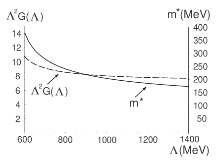
Figure 1: The running NJL coupling constant $G$ (dashed line) and the running constituent mass $m^{*}$ (in MeV, solid line) as functions of $\Lambda$ (in MeV). $\Lambda$ is the ultraviolet cutoff. The vertical axis on the left refers to $\Lambda^{2}G(\Lambda)$, while the axis on the right refers to $m^{*}$.

Our choice implies that a NJL model is defined at any scale by using the appropriate $G(\Lambda)$. Whereas in the usual case we have to keep the momenta smaller than the cutoff, now, for any given momenta, we can fix the cutoff in such a way that it is much bigger than the momenta. The phenomenology of the chiral world is clearly unaffected by this procedure; in fact it turns out that the constituent mass acquires a weak dependence on the cutoff, and therefore it can be fixed at the most convenient value. Also the quantity $G(\Lambda)\Lambda^{2}$ decreases weakly with the cutoff. In applying these considerations to the calculations at finite density, we have only to use the appropriate value of the coupling as given by $G(\mu+\delta)$, where now $\mu+\delta$ has nothing to do with the value of $\Lambda$ chosen to fit the chiral world. To give an explicit example we consider the CFL phase with massless quarks. There are two independent gaps $\Delta$ and $\Delta_{9}$ ($\Delta_{9}=-2\Delta$ if the pairing is only in the antitriplet channel) and the gap equations are [3, 13]:

$$\Delta = -\,\frac{\mu^{2}G}{6\pi^{2}}\left(\Delta_{9}\ {\rm arcsinh}\frac{\delta}{|\Delta_{9}|}-2\Delta\ {\rm arcsinh}\frac{\delta}{|\Delta|}\right)\,,$$ (4)

$$\Delta_{9} = -\,\frac{4\mu^{2}G\Delta}{3\pi^{2}}\ {\rm arcsinh}\frac{\delta}{|\Delta|}\ .$$ (5)

If one uses a fixed value for $\Lambda=\mu+\delta$, as for instance in ref. [18], one gets a non monotonic behavior of the gap, as it can be seen from fig. 2, (dashed line); a similar behavior was found in [18] (their fig. 1), albeit a different choice of the parameters produces some numerical differences.

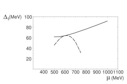
Figure 2: The CFL gap $\Delta$ for massless quarks, as obtained from eq. 5, versus the quark chemical potential for the two cases discussed in the text. Solid line: running NJL coupling $G(\mu+\delta)$ and cutoff $\delta=c\mu$, with $c=0.35$; dashed line: $\delta=\Lambda-\mu$, where $\Lambda=800$ MeV, and $G(\Lambda)=13.3$ GeV^-2. The picture shows the different qualitative behavior with $\mu$ of the gap.

On the other hand the solid line shows an increasing behavior of the gap. We see that in this way one reproduces qualitatively the behavior found in QCD for asymptotic chemical potential [16]. This result is obtained by the running NJL coupling $G(\mu+\delta)$, with the following choice of the cutoff $\delta$:

$$\delta=c\,\mu$$ (6)

with $c$ a fixed constant ($c=0.35$ in fig. 2). The reason for this choice is that, as discussed above, when increasing $\mu$, we do not want to reduce the ratio of the number of the relevant degrees of freedom to the volume of the Fermi sphere. Requiring the fractional importance to be constant is equivalent to require eq. (6).

In fig. 3, we plot the gap parameter $\Delta_{1}$ (the results for $\Delta_{9}$ are similar) as a function of $c$ for three different values of the chemical potential. In general there exists a window of values for $c$:

$$c=0.35\pm 0.10\ ,$$ (7)

where the gap parameters are less dependent on $c$. This is therefore the range of $c$ we shall assume below.

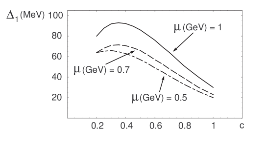
Figure 3: Gap parameter $\Delta_{1}$ as a function of $c$, where $\delta=c\,\mu$; the quarks are massless. The three curves are obtained for three values of the quark chemical potential: $\mu=1.0,\,0.7,\,0.5$ GeV.

It can be also noted that the result for the QCD superconducting model we are considering here has its counterpart in solid state physics, where the analysis of [19] shows a linear increase of $\delta$ with $\mu$ similar to eq. (6).

These results, valid for the massless case, are confirmed by a complete numerical analysis including the effect of a strange mass. This will be discussed in the subsequent section.

3 Effective lagrangian for gapless quarks

The massive case is considerably more involved, and the simple set of equations (5) has to be substituted by a system of 5 equations [5] that can be only solved numerically. In [18] the CFL phase with massive strange quark was also considered. In comparison with [5] the derivation we present here has the advantage of offering semi-analytical results, thanks to an expansion in powers of $m_{s}/\mu$. We principally differ from ref. [18] for the different treatment of the cutoff, as discussed in the previous section, and for the inclusion of pairing in both the antitriplet and the sextet color channel. The possibility of a semi-analytical treatment rests on the HDET approximation. This effective lagrangian approach was extended in [14] to the 2SC phase with massive quarks and here we treat the three flavor case.

In the HDET one introduces effective velocity dependent fields, corresponding to the positive energy solutions of the field equations: $\psi_{\alpha,i,\vec{n}}(x)$ where $\alpha,\,i$ are color and flavor indices, $\vec{n}=\vec{v}/|\vec{v}|$, and $\vec{v}$ is the quark velocity defined by the equation

$$p^{\mu}=\mu v^{\mu}+\ell^{\mu}$$ (8)

with $v^{\mu}=(0,\vec{v})$. The effective fields $\psi_{\alpha,i\,\vec{n}}(x)$ are expressed in terms of Fourier-transformed quark fields $\tilde{\psi}_{\alpha,i}(p)$ as follows

$$\psi_{\alpha,i\,\vec{n}}(x)={\cal P}_{+}\int\frac{d^{4}p}{(2\,\pi)^{4}}\,e^{i\,(p-\mu v)\cdot x}\,\tilde{\psi}_{\alpha,i}(p)\ .$$ (9)

Here ${\cal P}_{+}$ is the positive energy projector, defined, together with ${\cal P}_{-}$, by the formula

$${\cal P}_{\pm}=\frac{1\pm(\vec{\alpha}\cdot\vec{v}+x_{i}\,\gamma^{0})}{2}\ ,$$ (10)

where $x_{i}=m_{i}/\mu$ and $m_{i}$ is the mass of the quark having flavor $i$. We now change the color-flavor basis introducing new fields $\psi^{A}_{\vec{n}}$ as follows:

$$\psi_{\alpha,i,\vec{n}}(x)\,=\,\sum_{A=1}^{9}\frac{\lambda^{A}_{\alpha i}}{\sqrt{2}}\,\psi^{A}_{\vec{n}}(x)\ ,$$ (11)

where $\lambda_{A}$ with $A=1,\dots,8$ are the usual Gell-mann matrices and $\lambda_{9}=\sqrt{2/3}\,\lambda_{0}$. We also introduce the Nambu-Gor’kov doublet

$$\chi_{A}=\frac{1}{\sqrt{2}}\left(\begin{array}[]{c}\psi^{A}_{\vec{n}}\\ C\,\psi^{A,*}_{-\vec{n}}\end{array}\right)\ .$$ (12)

In the $\chi_{A}$ basis the lagrangian of the quarks, including the quark-gluon interaction and the gap therm can be written in momentum space as follows:

$${\cal L}={\cal L}_{0}+{\cal L}_{1}+{\cal L}_{\Delta}\ .$$ (13)

${\cal L}_{0}$ is the kinetic term while ${\cal L}_{1}$ describes the quark-gluon interaction. They are given by:

$${\cal L}_{0} = \sum_{\vec{n}}\sum_{A,B=1}^{9}\,\chi_{A}^{\dagger}\,\left(\begin{array}[]{cc}{\bf\,V_{AB}\cdot\ell}&0\\ 0&{\bf\,\tilde{V}_{AB}\cdot\ell}\end{array}\right)\,\chi_{B}\ ,$$ (16)

$${\cal L}_{1} = \,ig\,\sum_{\vec{n}}\sum_{A,B=1}^{9}\,\chi_{A}^{\dagger}\,\left(\begin{array}[]{cc}{\bf H_{AB}\cdot}A&0\\ 0&-{\bf\tilde{H}_{AB}}^{*}\cdot A\end{array}\right)\,\chi_{B}\ .$$ (19)

We have introduced the symbols

$${\bf\,V_{AB}\cdot\ell} = Tr\left[T_{A}\,T_{B}\,{\cal V}^{\mu}\right]\ell_{\mu}~{},~{}~{}~{}~{}~{}~{}~{}~{}~{}~{}~{}~{}~{}{\bf\tilde{V}_{AB}\cdot\ell}=Tr\left[T_{A}\,T_{B}\,\tilde{\cal V}^{\mu}\right]\ell_{\mu}$$ (20)

$${\bf\,H_{AB}\cdot}A = H^{\mu}_{AmB}\cdot A^{m}_{\mu}=\,\frac{1}{\sqrt{2}}\,Tr\left[T_{A}\,T_{m}\,T_{B}\,{\cal V}^{\mu}\right]A^{m}_{\mu}~{},$$ (21)

$${\bf\tilde{H}_{AB}\cdot}A = {\tilde{H}}^{\mu}_{AmB}\cdot A^{m}_{\mu}=\,\frac{1}{\sqrt{2}}\,Tr\left[T_{A}\,T_{m}\,T_{B}\,\tilde{\cal V}^{\mu}\right]A^{m}_{\mu}\ .$$ (22)

In these equations $T_{A}=\lambda_{A}/\sqrt{2}$, $A^{m}_{\mu}$ is the gluon field, and ${\cal V}^{\mu}$ denotes the matrix

$${\cal V}^{\mu}_{ij}=\left(\begin{array}[]{ccc}{\cal V}^{\mu}_{u}&0&0\\ 0&{\cal V}^{\mu}_{d}&0\\ 0&0&{\cal V}^{\mu}_{s}\end{array}\right)$$ (23)

with ${\cal V}^{\mu}_{i}=(1,\,\vec{v}_{i})$ for each flavor $i$; a similar definition holds for $\tilde{\cal V}^{\mu}_{ij}$, with $\tilde{\cal V}^{\mu}_{i}=(1,\,-\,\vec{v}_{i})$. In the limit $m_{u}=m_{d}\approx 0$ one has $v_{u}=v_{d}=1\ ,~{}~{}~{}v_{s}=\sqrt{1-x_{s}^{2}}=\sqrt{1-m_{s}^{2}/\mu_{s}^{2}}$.

Let us now turn to the gap term ${\cal L}_{\Delta}$. We consider CFL condensation in both the antisymmetric $\bar{\bf 3}_{A}$ and in the symmetric ${\bf 6}_{S}$ channels. We assume equal masses (actually zero) for the up and down quarks and neglect quark-antiquark chiral condensates, whose contribution is expected to negligible in the very large $\mu$ limit. Also the contribution from the repulsive ${\bf 6}_{S}$ channel is expected to be small, but we include it because the gap equations are consistent only with condensation in both the ${\bf 6}_{S}$ and the $\bar{\bf 3}_{A}$ channels. The condensate we consider is therefore

$$<\psi_{\alpha i}\,C\,\gamma_{5}\,\,\psi_{\beta j}>\sim\left(\Delta_{ij}\,\epsilon^{\alpha\beta I}\epsilon_{ijI}+G_{ij}\,(\delta^{\alpha i}\,\delta^{\beta j}+\delta^{\alpha j}\,\delta^{\beta i})\right)\ .$$ (24)

The first term on the r.h.s accounts for the condensation in the $\bar{\bf 3}_{A}$ channel and the second one describes condensation in ${\bf 6}_{S}$ channel. As we assume $m_{u}=m_{d}$, we put

$$\Delta_{us}=\Delta_{ds}\equiv\Delta\ ,~{}~{}~{}~{}~{}~{}~{}~{}~{}~{}~{}~{}\Delta_{ud}\equiv\Delta_{12}\ ,$$ (25)

$$G_{uu}=G_{du}=G_{ud}=G_{dd}\equiv G_{1}\ ,~{}~{}~{}~{}~{}~{}~{}~{}~{}~{}~{}~{}G_{us}=G_{ds}\equiv G_{2}\ ,~{}~{}~{}~{}~{}~{}~{}~{}~{}~{}~{}G_{ss}\equiv G_{3}\ ,$$ (26)

which reduces the number of independent gap parameters to five. We stress that we impose electrical and color neutrality, which, as shown in ref. [7], is indeed satisfied in the color-flavor locked phase of QCD because in this phase the three light quarks number densities are equal $n_{u}=n_{d}=n_{s}$, with no need for electrons, i.e. $n_{e}=0$. As a consequence, the Fermi momenta of the three quarks are equal:

$$p_{F,\,u}\,=\,p_{F,\,d}\,=\,p_{F,\,s}\,\equiv\,p_{F}\,\ ,$$ (27)

which, in terms of the quark chemical potentials and Fermi velocities can be written as

$$\mu_{u}|\vec{v}_{u}|\,=\,\mu_{d}|\vec{v}_{d}|\,=\,\mu_{s}|\vec{v}_{s}|\ .$$ (28)

It follows that the wave function of the quark-quark condensate has no dependence on the Fermi energies and the condensation can be described in the mean field approximation by the following lagrangian term containing only the effective fields $\psi_{\alpha i,\,\pm}$:

$${\cal L}_{\Delta}=-\frac{\Delta_{ij}\,\epsilon^{\alpha\beta I}\epsilon_{ijI}+G_{ij}\,(\delta^{\alpha i}\,\delta^{\beta j}+\delta^{\alpha j}\,\delta^{\beta i})}{2}\,\sum_{\vec{n}}\,\psi^{T}_{\alpha i,\,-}\,C\,\gamma_{5}\,\psi_{\beta j,\,+}\,+\,h.c.$$ (29)

Using the Nambu-Gor’kov fields one rewrites (29) as follows:

$${\cal L}_{\Delta}=\sum_{\vec{n}}\sum_{A,B=1}^{9}\,\chi_{A}^{\dagger}\,\left(\begin{array}[]{cc}0&\gamma_{5}\,\otimes\,{\bf\Delta_{AB}}\\ \gamma_{5}\,\otimes\,{\bf\Delta_{AB}^{\dagger}}&0\end{array}\right)\,\chi_{B}$$ (30)

where

$${\bf\Delta_{AB}}={\bf\Delta_{AB}}({\bar{\bf 3}})+{\bf\Delta_{AB}}({\bf 6})$$ (31)

and

$${\bf\Delta_{AB}}({\bar{\bf 3}})=\left(\begin{array}[]{cccc}\Delta_{12}\,I_{3}&0&0&0\\ 0&\Delta\,I_{4}&0&0\\ 0&0&\frac{1}{3}\left(4\,\Delta-\Delta_{12}\right)&\frac{\sqrt{2}}{3}\left(\Delta-\Delta_{12}\right)\\ 0&0&\frac{\sqrt{2}}{3}\left(\Delta-\Delta_{12}\right)&-\frac{2}{3}\left(\Delta_{12}+2\,\Delta\right)\end{array}\right)$$ (32)

$${\bf\Delta_{AB}}({\bf 6})=\left(\begin{array}[]{cccc}G_{1}\,I_{3}&0&0&0\\ 0&G_{2}\,I_{4}&0&0\\ 0&0&G_{1}-\frac{4}{3}(G_{2}-G_{3})&\frac{\sqrt{2}}{3}(3G_{1}-2G_{3}-G_{2})\\ 0&0&\frac{\sqrt{2}}{3}(3G_{1}-2G_{3}-G_{2})&\frac{2}{3}(3G_{1}+2G_{2}+G_{3})\end{array}\right)\ ,\\$$ (33)

where $I_{n}$ stays for the $n\times n$ identity matrix. The nine eigenvalues of the matrix ${\bf\Delta_{AB}}$ are reported in the Appendix. From the lagrangian

$${\cal L}_{0}\,+\,{\cal L}_{\Delta}=\sum_{\vec{n}}\sum_{A,B=1}^{9}\,\chi_{A}^{\dagger}\,\left(\begin{array}[]{cc}{\bf\,V_{AB}\cdot\ell}&\gamma_{5}\,\otimes\,{\bf\Delta_{AB}}\\ \gamma_{5}\,\otimes\,{\bf\Delta_{AB}^{\dagger}}&{\bf\,\tilde{V}_{AB}\cdot\ell}\end{array}\right)\,\chi_{B}\,=\sum_{\vec{n}}\sum_{A,B=1}^{9}\,\chi_{A}^{\dagger}S^{-1}_{AB}(\ell)\chi_{B}$$ (34)

the fermionic propagator is obtained:

$$S_{AB}(\ell)=\left(\begin{array}[]{cc}{\bf\frac{\displaystyle 1}{\displaystyle\Delta\tilde{V}\cdot\ell\Delta^{-1}\,V\cdot l-\Delta^{2}}\,\Delta\tilde{V}\cdot\ell\Delta^{-1}}&{\bf-\frac{\displaystyle 1}{\displaystyle\Delta\,\tilde{V}\cdot\ell\,\Delta^{-1}\,V\cdot l-\Delta^{2}}\,\gamma_{5}\,\otimes\,\Delta}\\ &\\ {\bf-\frac{\displaystyle 1}{\displaystyle\Delta V\cdot\ell\,\Delta^{-1}\,\tilde{V}\cdot l-\Delta^{2}}\,\gamma_{5}\,\otimes\Delta}&{\bf\frac{\displaystyle 1}{\displaystyle\Delta V\cdot\ell\,\Delta^{-1}\tilde{V}\cdot l-\Delta^{2}}\,\Delta V\cdot\ell\,\Delta^{-1}}\end{array}\right)_{AB}$$

The off-diagonal matrix $S_{AB}^{12}$ (1, 2= NG indices) is the anomalous component of the quark propagator, which is what we need to write down the gap equations. In matrix form they are as follows

$$-{\bf\Delta_{AB}}=-\frac{i\,G(\mu+\delta)\,p_{F}^{2}}{4\,\pi^{3}}\,H_{AaC}^{\mu}\,H_{DbB}^{\nu*}\,\int_{-\delta}^{+\delta}d\ell_{\parallel}\int_{-\infty}^{+\infty}d\ell_{0}\delta^{ab}\,g_{\mu\nu}\,S^{12}_{CD}(l)\,,$$ (35)

where the color-flavor symbols $H_{AaB}^{\mu}$ have been defined in (22) and the running NJL coupling is computed at $\mu+\delta$, according to the previous discussion. In eq. (35) $\delta=c\mu$ is the cutoff discussed in section 2. The gap equations can be numerically solved; results for $m_{s}=250$ MeV and $c=0.35$ are reported in Fig. 4.

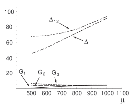
Figure 4: The five gap parameters vs. the chemical potential $\mu$; results obtained by the numerical solution of the exact gap equations, for $m_{s}=250$ MeV and $\delta=0.35\mu$. The upper curve refers to $\Delta_{12}$, while the middle one refers to $\Delta$. The lower curves are the data obtained for the three sextet gap parameters $|G_{1}|$, $|G_{2}|$ and $|G_{3}|$. Gaps and $\mu$ are expressed in MeV.

A semi-analytical solution can be found by performing an expansion in the strange quark mass:

$$x_{s}=\frac{m_{s}}{\mu_{s}}\approx\frac{m_{s}}{\mu}\ll 1\ .$$ (36)

Here $\mu=\mu_{u}=\mu_{d}$, $\mu_{s}=\mu+\delta\mu$ with $\delta\mu={\cal O}(m_{s}/\mu)^{2}$. We define:

$$\Delta_{1} = \Delta_{12}+G_{1}\equiv\Delta^{0}_{1}+\epsilon_{1}x_{s}^{2}~{},~{}~{}~{}~{}\Delta_{9}=-\,2\,\Delta_{12}+4\,G_{1}\equiv\Delta^{0}_{9}+\epsilon_{9}x_{s}^{2}\,,$$ (37)

$$\Delta \equiv \frac{4\Delta_{1}^{0}-\Delta_{9}^{0}}{6}-\xi_{1}x_{s}^{2}~{},~{}~{}G_{2}\equiv\frac{2\Delta_{1}^{0}+\Delta_{9}^{0}}{6}-\xi_{2}x_{s}^{2}~{},~{}~{}G_{3}\equiv\frac{2\Delta_{1}^{0}+\Delta_{9}^{0}}{6}-\xi_{3}x_{s}^{2}\ ,$$ (39)

where $\Delta^{0}_{1},\Delta^{0}_{9}$ are the values for massless quarks and can be obtained from eqns. (5). For $m_{s}\neq 0$ the number of gaps increases from 2 to 5, but eqns. (39) give immediately the solutions for any value of $m_{s}$ (with the proviso $x_{s}=m_{s}^{2}/\mu^{2}\ll 1$) if one knows the parameters $\xi=(\epsilon_{1},\epsilon_{9},\xi_{1},\xi_{2},\xi_{3})$. They can be obtained by solving the system of 5 linear algebraic equations

$${\bf A}\cdot{\bf\xi}={\bf f}\ .$$ (40)

The matrices ${\bf A}$ and $f$ are reported in the appendix. Numerical results for the parameters $\bf\xi$ are in Table 1. For a strange mass of $250$ MeV we find the rate $\Delta_{9}/\Delta_{1}$ equal to $-2.365$ for $\mu=500$ MeV and $-2.33$ for $\mu=1000$ MeV.

$\mu$	$\epsilon_{1}$	$\epsilon_{9}$	$\xi_{1}$	$\xi_{2}$	$\xi_{3}$
500	-35.29	90.48	33.63	-2.06	-6.20
700	-44.86	102.93	41.16	-3.10	-8.72
1000	-61.21	135.08	55.69	-4.42	-12.23

Table 1: Values of the ${\xi}$ components, obtained by means of the $5\times 5$ system of linear equations. In the gap equations we have made the choice $\delta=0.35\,\mu$. All the gaps and $\mu$’s are expressed in MeV.

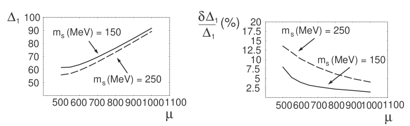
Figure 5: Gap parameter $\Delta_{1}=\Delta_{12}+G_{1}$ as a function of $\mu$. Left panel: results for two different values of the strange quark mass, $m_{s}=150,\,250$ MeV (curves are obtained by means of the perturbative gap equations). Right panel: relative variation $\delta\Delta_{1}/\Delta_{1}=[\Delta_{1}(m_{s})-\Delta_{1}(0)]/\Delta_{1}(0)$. In this plot $\delta=0.35\mu$. Gaps and $\mu$’s are expressed in MeV.

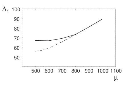
Figure 6: This diagram shows the difference between the exact numerical calculation of the gap $\Delta_{1}$ for $m_{s}=250$ MeV (solid line) and the approximate result obtained through the expansion in $m_{s}$ (dashed line). Units are MeV.

From these results we can compute the dependence of the various gaps on $\mu$. For $\Delta_{1}$ it is reported (for two values of the strange quark mass) in fig.5. We stress that the approximation we consider here is indeed very good in the range of parameters we have considered in the present paper, i.e. $m_{s}=150-250$ MeV and $\mu=500-1000$ MeV. As an example, fig. 6 shows the approximate solution for $\Delta_{1}$ (solid line), which differs only by a few percent from the exact solution (dashed line), except in the lower region of $\mu$. These results are obtained for a mass of 250 MeV; for smaller values the effect is even less relevant.

4 Conclusions

A main point in this work has been to clarify the issue of the dependence on $\mu$ of the ultraviolet cutoff in the NJL model and its application to CFL phase of QCD. A convenient procedure consists in re-defining the NJL coupling such as to make it cutoff dependent. The application to the CFL model with $m_{s}\not=0$ leads, in the approximation of the high density effective theory, to an expansion in the parameter $(m_{s}/\mu)^{2}$, whose numerical validity is very good already at first order. Both triplet and sextet gaps are included. The gap parameters are obtained as functions of the chemical potential and their behavior is consistent with the expected asymptotic limits.

Appendix

Eigenvalues of the gap matrix

The eigenvalues of the gap matrix for CFL with massive strange quark are as follows: $\Delta_{1}=\dots=\Delta_{5}=\Delta_{12}+G_{1}$, $\Delta_{6}=\Delta_{7}=\Delta+G_{2}$, $\Delta_{8/9}=\frac{1}{2}\left(x-z\pm\sqrt{(x+z)^{2}+4y^{2}}\right)$ where $x,y,z$ are given by

$$x = \frac{1}{3}(4\Delta-\Delta_{12})+G_{1}-\frac{4}{3}(G_{2}-G_{3})\,,$$ (41)

$$y = \frac{\sqrt{2}}{3}(\Delta-\Delta_{12})+\sqrt{2}\left(G_{1}-\frac{G_{2}}{3}-\frac{\sqrt{2}G_{3}}{3}\right)\,,$$ (42)

$$z = \frac{2}{3}(\Delta_{12}+2\Delta)-\frac{2}{3}(3G_{1}+2G_{2}+G_{3})\,.$$ (43)

Matrices ${\bf\xi}$, ${\bf A}$, $\bf f$

We write down explicitly the matrices ${\bf\xi}$, ${\bf A}$, $\bf f$ defined in the text

$${\bf\xi}^{T}=\left(\epsilon_{1}\ \epsilon_{9}\ \xi_{1}\ \xi_{2}\ \xi_{3}\right)\ ;$$ (44)

$${\bf A}=\left(\begin{array}[]{ccccc}\alpha&\beta&-\frac{2}{9}b(-g_{1}+2g_{9}-g_{19})&\frac{2}{9}b(-g_{1}+2g_{9}-g_{19})&\frac{2}{9}b(g_{1}-g_{9}+2g_{19})\\ \alpha&\beta&-1-\frac{b}{9}(7g_{1}+4g_{9}+g_{19})&-1+\frac{b}{9}(g_{1}+4g_{9}+g_{19})&-\frac{b}{9}(4g_{1}+2g_{9}+2g_{19})\\ \alpha&\beta&-\frac{4}{3}-\frac{2b}{9}(5g_{1}+2g_{9}+g_{19})&\frac{4}{3}-\frac{2b}{9}(7g_{1}-2g_{9}-g_{19})&-\frac{4}{3}-\frac{2b}{9}(-g_{1}+g_{9}+2g_{19})\\ 0&0&-\frac{\sqrt{2}}{3}\left(1+\frac{b}{3}(5g_{1}-g_{19})\right)&\frac{\sqrt{2}}{3}\left(1-\frac{b}{3}(g_{1}-g_{19})\right)&-\frac{2\sqrt{2}}{3}\left(1+\frac{b}{3}(g_{1}-g_{19})\right)\\ \gamma&1&\frac{4}{3}-\frac{2b}{9}4g_{1}&-\frac{4}{3}-\frac{16b}{9}g_{1}&\frac{2}{3}+\frac{4b}{9}g_{1}\end{array}\right)$$ (45)

where we have defined $b=G(\mu+\delta)\mu^{2}/2\pi^{2}$, $\alpha=1-\frac{2}{3}b\,h_{1}$, $\beta=\frac{1}{3}b\,h_{9}$, $\gamma=\frac{8b}{3}h_{1}$; finally

$${\bf f}=\left(\begin{array}[]{c}b\left(-\frac{\tilde{I}^{0}_{1}}{3}+\frac{\tilde{I}^{0}_{9}}{6}-\frac{1}{18}(f_{1}+f_{9}-4f_{19})\right)\cr b\left(-\frac{\tilde{I}^{0}_{1}}{2}+\frac{\tilde{I}^{0}_{9}}{4}-\frac{1}{18}(5f_{1}-f_{9}-2f_{19})\right)\cr b\left(\frac{5}{18}\left(-2\tilde{I}^{0}_{1}+2\tilde{I}^{0}_{9}\right)+\frac{1}{18}(11f_{1}-f_{9}-4f_{19})\right)\\ b\left(\frac{1}{18\sqrt{2}}(-7\tilde{I}^{0}_{1}-\tilde{I}^{0}_{9})+\frac{\sqrt{2}}{18}(\frac{17}{2}f_{1}+f_{19}))\right)\cr b\left(\frac{16}{9}\tilde{I}^{0}_{1}+\frac{10}{18}f_{1}\right)\end{array}\right)\ .$$ (46)

The values of the parameters $f_{j}$, $g_{j}$, $\tilde{I}^{0}_{j}$, $h_{k}$ are listed below.

$$f_{1} = \frac{1}{2\pi i}\Delta^{0}_{1}J^{\delta}(\Delta^{0}_{1})~{},~{}~{}~{}f_{9}=\frac{1}{2\pi i}\Delta^{0}_{9}J^{\delta}(\Delta^{0}_{9})~{},~{}~{}~{}f_{19}=\frac{1}{2\pi i}\Delta^{0}_{1}J^{\delta}(\Delta^{0}_{1},\Delta^{0}_{9})\ ,$$ (47)

$$g_{1} = \frac{1}{2\pi i}I^{\delta}(\Delta^{0}_{1})~{},~{}~{}~{}g_{9}=\frac{1}{2\pi i}I^{\delta}(\Delta^{0}_{9})~{},~{}~{}~{}g_{19}=\frac{1}{2\pi i}I^{\delta}(\Delta^{0}_{1},\Delta^{0}_{9})\ ,$$ (49)

$$\tilde{I}^{0}_{j} = \Delta^{0}_{j}{\rm arcsinh}\left|\frac{\delta}{\Delta^{0}_{j}}\right|~{},~{}~{}~{}h_{k}={\rm arcsinh}\left|\frac{\delta}{\Delta^{0}_{j}}\right|-1\ .$$ (50)

In this expression we use the following parametric integrals:

$$I^{\delta}(x) = \int_{-\delta}^{\delta}d^{2}l\,\frac{V\cdot l\,\tilde{V}\cdot l+x^{2}}{D(x)^{2}}=2\,\pi\,i\left(-{\rm arcsinh}\left|\frac{\delta}{x}\right|+\frac{\delta}{\sqrt{\delta^{2}+x^{2}}}\right)\ ,$$ (51)

$$I^{\delta}(x_{1},x_{2}) = \int_{-\delta}^{\delta}d^{2}l\,\frac{V\cdot l\,\tilde{V}\cdot l+x_{1}\,x_{2}}{D(x_{1})\,D(x_{2})}=$$ (52)

$$= \frac{2\,\pi}{i}\left[{\rm arcsinh}\left|\frac{\delta}{x_{2}}\right|+\frac{x_{1}(x_{1}+x_{2})}{x_{2}^{2}-x_{1}^{2}}\left({\rm arcsinh}\left|\frac{\delta}{x_{2}}\right|-{\rm arcsinh}\left|\frac{\delta}{x_{1}}\right|\right)\right]\ ,$$

$$J^{\delta}(x) = \int_{-\delta}^{\delta}d^{2}l\,\frac{l_{\parallel}^{2}}{D(x)^{2}}=i\,\pi\left({\rm arcsinh}\left|\frac{\delta}{x}\right|-\frac{\delta}{\sqrt{\delta^{2}+x^{2}}}\right)\,,$$ (53)

$$J^{\delta}(x_{1},x_{9}) = \int_{-\delta}^{\delta}d^{2}l\,\frac{l_{\parallel}^{2}}{D(x_{1})D(x_{9})}=\frac{i\,\pi}{2(x_{1}^{2}-x_{9}^{2})}\left[-2\,\delta\left(\sqrt{x_{1}^{2}+\delta^{2}}-\sqrt{x_{9}^{2}+\delta^{2}}\right)\right.$$ (54)

$$\left.+2\,x_{1}^{2}\,{\rm arcsinh}\left|\frac{\delta}{x_{1}}\right|-2\,x_{9}^{2}\,{\rm arcsinh}\left|\frac{\delta}{x_{9}}\right|\right]\ .$$

Acknowledgements

We wish to thank M. Mannarelli for useful discussions. One of us, G. N., wishes to thank the CERN theory group for the very kind hospitality.

References

[1]
K. Rajagopal and F. Wilczek,
[arXiv:hep-ph/0011333].
[2]
M. Alford, Ann. Rev. Nucl. Part. Sci.51 (2001) 131
[arXiv:hep-ph/0102047].
[3]
M. G. Alford, K. Rajagopal and F. Wilczek,
Phys. Lett. B 422 (1998) 247 [arXiv:hep-ph/9711395].
[4]
R. Rapp, T. Schaefer, E. V. Shuryak and M. Velkovsky,
Phys. Rev. Lett. 81 (1998) 53 [arXiv:hep-ph/9711396].
[5]
M. G. Alford, J. Berges and K. Rajagopal,
Nucl. Phys. B 558 (1999) 219 [arXiv:hep-ph/9903502].
[6]
T. Schaefer and F. Wilczek,
Phys. Rev. D 60 (1999) 074014 [arXiv:hep-ph/9903503].
[7]
K. Rajagopal and F. Wilczek,
Phys. Rev. Lett. 86, 3492 (2001) [arXiv:hep-ph/0012039].
[8]
P. Amore, M. C. Birse, J. A. McGovern and N. R. Walet,
Phys. Rev. D 65 (2002) 074005 [arXiv:hep-ph/0110267].
[9]
M. Alford and K. Rajagopal,
JHEP 0206 (2002) 031 [arXiv:hep-ph/0204001].
[10]
D. K. Hong,
Phys. Lett. B 473 (2000) 118 [arXiv:hep-ph/9812510];
D. K. Hong,
Nucl. Phys. B 582 (2000) 451 [arXiv:hep-ph/9905523].
[11]
S. R. Beane, P. F. Bedaque and M. J. Savage,
Phys. Lett. B 483 (2000) 131 [arXiv:hep-ph/0002209].
[12]
R. Casalbuoni, R. Gatto and G. Nardulli,
Phys. Lett. B 498 (2001) 179 [Erratum-ibid. B 517
(2001) 483] [arXiv:hep-ph/0010321].
[13]
G. Nardulli,
Riv. Nuovo Cim. 25N3 (2002) 1 [arXiv:hep-ph/0202037].
[14]
R. Casalbuoni, F. De Fazio, R. Gatto, G. Nardulli and M. Ruggieri,
Phys. Lett. B 547 (2002) 229 [arXiv:hep-ph/0209105].
[15]
M. G. Alford, J. Berges and K. Rajagopal,
Phys. Rev. Lett. 84 (2000) 598 [arXiv:hep-ph/9908235].
[16]
D. T. Son,
Phys. Rev. D 59 (1999) 094019 [arXiv:hep-ph/9812287].
[17]
S. P. Klevansky,
Rev. Mod. Phys. 64 (1992) 649.
[18]
A. W. Steiner, S. Reddy and M. Prakash,
Phys. Rev. D 66, 094007 (2002) [arXiv:hep-ph/0205201].
[19]L. P. Gorkov, T. K. Melik-Barchudarov, Zh. Eksp. Teor. Fiz. 40 (1961)
1452.