CERN-TH/2003-018

Multiphoton Radiation in Leptonic $W$-Boson Decays^⋆

W. Płaczek^a,b  and  S. Jadach^c,b

^aInstitute of Computer Science, Jagellonian University,
ul. Nawojki 11, 30-072 Cracow, Poland,
^bCERN, TH Division, CH-1211 Geneva 23, Switzerland,
^cInstitute of Nuclear Physics,
ul. Radzikowskiego 152, 31-342 Cracow, Poland,

We present the calculation of multiphoton radiation effects in leptonic $W$-boson decays in the framework of the Yennie–Frautschi–Suura exclusive exponentiation. This calculation is implemented in the Monte Carlo event generator WINHAC for single $W$-boson production in hadronic collisions at the parton level. Some numerical results obtained with the help of this program are also presented.

To be submitted to European Physical Journal C

• Work partly supported by the Polish Government grants KBN 2P03B00122 and KBN 5P03B09320, the EC FP5 contract HPRN-CT-2000-00149, the EC FP5 Centre of Excellence “COPIRA” under the contract No. IST-2001-37259.

CERN-TH/2003-018
January 2003

1 Introduction

Studying the $W$-boson physics is an important way of testing the Standard Model (SM) and searching for “new physics”. It can be done in both the electron–positron and hadron colliders. In $e^{+}e^{-}$ collisions, the main source of $W$ bosons is the process of $W$-pair production. This process was one of the most important subjects of the LEP2 experiments at CERN, run in the years 1996–2000, see e.g. Refs. [1, 2]. It also belongs to the main topics of a research programme of future linear colliders (LC), see e.g. Ref. [3]. In this process one can measure precisely the $W$-boson mass and width as well as non-abelian triple and quartic gauge-boson couplings. In hadron colliders (proton–proton or proton–antiproton), the main source of $W$ bosons is the process of single-$W$ production. The most precise measurements of the $W$-boson mass and width in hadron colliders come from this process, see e.g. Ref. [4]. It can also be used to extract parton distribution functions (PDFs) and to measure parton luminosities [5].

Among radiative corrections that affect the $W$-boson observables considerably is the photon radiation in leptonic $W$ decays. It distorts $W$-invariant-mass distributions reconstructed from $W$-decay products in $e^{+}e^{-}$ experiments [6, 7] or $W$-transverse-mass distributions obtained in hadron-collider experiments [8]. These distortions are strongly acceptance-dependent, see e.g. Refs. [8, 7]. This radiation also affects lepton pseudorapidity distribution, which is the main tool for the PDFs and parton luminosities measurements in the hadron colliders. Therefore, precise theoretical predictions for the photon radiation in the leptonic $W$ decays is of great importance for both types of high-energy particle colliders. In order to be fully applicable in a realistic experimental situation, such predictions have to be provided in terms of a Monte Carlo event generator (MCEG).

The ${\cal O}(\alpha)$ electroweak (EW) radiative corrections in the on-shell $W$ decays were calculated analytically a long time ago by several authors [9, 10, 11, 12]. In the case of the $W$-pair production in the $e^{+}e^{-}$ colliders, the calculations of the ${\cal O}(\alpha)$ EW corrections in a double-pole approximation (DPA) were done in Refs. [13] and [14]. The latter were implemented in the MCEG RacoonWW [14]. For single-$W$ production in hadronic collisions, the respective ${\cal O}(\alpha)$ EW corrections were calculated in Refs. [15, 8, 16, 17]. The MCEG for this process, including pure QED ${\cal O}(\alpha)$ corrections, was provided long ago by Berends and Kleiss [18]. A two-real-photon radiation cross section in $W$ decays was calculated in Ref. [19]. On the other hand, the MC package PHOTOS [20] provides a universal tool for the generation of photon radiation in particle decays up to ${\cal O}(\alpha^{2}$) in the leading-log (LL) approximation. It was used in the MCEG YFSWW [21] for the simulation of radiative $W$ decays for the $W$-pair production process in $e^{+}e^{-}$ collisions.

To date, however, none of the existing MCEG for $W$-boson physics included multiphoton radiation in leptonic $W$ decays through exclusive QED exponentiation. Therefore, the influence of higher-order radiative corrections on the $W$-boson observables was difficult to assess. In this paper, we provide the first calculation of the multiphoton radiation in leptonic $W$ decays in the framework of the Yennie–Frautschi–Suura exclusive exponentiation [22]. This calculation is implemented in the MCEG for single-$W$ production in quark–antiquark collisions called WINHAC [23]. It is a starting point for the full MC program for Drell–Yan-like single-$W$ production at the proton–antiproton (Tevatron) and proton–proton (LHC) colliders. The presented calculation as well as the respective MC algorithm can also be implemented in the MCEG for $W$-pair production in the $e^{+}e^{-}$ collisions, such as YFSWW.

The paper is organized as follows. In Section 2 we provide spin amplitudes for the Born-level process and for the process with single-photon radiation in $W$ decays. In Section 3 we discuss the YFS exponentiation in leptonic $W$-boson decays. Numerical results are presented in Section 4. Section 5 summarizes the paper and gives some outlook. Finally, the appendices contain supplementary formulae.

2 Spin amplitudes

In the calculation of matrix elements for the process of single-$W$ production in hadronic collisions, we use the spin amplitude formalism of Ref. [24]. In this approach, spinors are expressed in the Weyl basis, the vector-boson polarizations in the Cartesian basis, and the spin amplitudes are evaluated numerically for arbitrary four-momenta and masses of fermions and bosons. This evaluation amounts, in practice, to multiplying 2$\times$2 $c$-number matrices by 2-dimensional $c$-number vectors. We give below the general spin amplitudes for arbitrary fermions in the initial and in the final states, and apply them later on to the single-$W$ production in $q\bar{q}$ collisions with leptonic $W$ decays.

2.1 Born level

Figure 1: The Born-level Feynman diagram for single-$W$ production in fermion–antifermion collisions.

The Born-level Feynman diagram for single-$W$ production in fermion–antifermion collisions

$$f_{1}(p_{1},\sigma_{1})+\bar{f_{2}}(p_{2},\sigma_{2})\longrightarrow W^{\pm}(Q,\lambda)$$ (1)

is depicted in Fig. 1, where $(p_{i},\sigma_{i})$ denotes the four-momentum and helicity ($\sigma_{i}=\pm 1$) of the corresponding fermion, while $(Q,\lambda)$ is the four-momentum and polarization of the $W$-boson ($\lambda=1,2,3$). The fermions $f_{1}$ and $f_{2}$ are members of $SU(2)_{L}$ doublets with opposite values of the weak-isospin third component and the pair $f_{1}\bar{f_{2}}$ is the $SU(3)_{c}$ singlet. The spin amplitudes for this process, in the convention of Ref. [24], read

$${\cal M}_{P}^{(0)}(\sigma_{1},\sigma_{2};\lambda)=-\frac{ieV_{f_{1}f_{2}}}{\sqrt{2}s_{W}}\,\omega_{-\sigma_{1}}(p_{1})\,\omega_{\sigma_{2}}(p_{2})\,\sigma_{2}\,S\left(p_{2},\epsilon_{W}^{\ast}(Q,\lambda),p_{1}\right)_{-\sigma_{2},\sigma_{1}}^{-},$$ (2)

where $e$ is the positron electric charge, $V_{f_{1}f_{2}}$ is the element of the weak-mixing matrix (the CKM matrix for quarks, the MNS matrix for leptons), $s_{W}=\sin\theta_{W}$, with $\theta_{W}$ the weak-mixing (Weinberg) angle;

$$\omega_{\pm}(p)=\sqrt{p^{0}\pm|\vec{p}|}\,;$$ (3)

$\epsilon_{W}(Q,\lambda)$ is the $W$-boson polarization vector ($\ast$ denotes the $c$-number conjugation); and $S(\ldots)$ is the spinorial string function, given explicitly in Appendix A. The above spin amplitudes are identical for any colour singlet of the initial fermion pair $f_{1}\bar{f_{2}}$.

Figure 2: The Born-level Feynman diagram for $W$-boson decay.

The spin amplitudes for the Born-level $W$-boson decay:

$$W^{\pm}(Q,\lambda)\longrightarrow f_{1}(q_{1},\tau_{1})+\bar{f_{2}}(q_{2},\tau_{2}),$$ (4)

shown diagrammatically in Fig. 2, are given by

$${\cal M}_{D}^{(0)}(\lambda;\tau_{1},\tau_{2})=-\frac{ieCV_{f_{1}f_{2}}}{\sqrt{2}s_{W}}\,\omega_{-\tau_{1}}(q_{1})\,\omega_{\tau_{2}}(q_{2})\,\tau_{2}\,S\left(q_{1},\epsilon_{W}(Q,\lambda),q_{2}\right)_{\tau_{1},-\tau_{2}}^{-},$$ (5)

where $\tau_{1,2}$ denote the helicities of the final-state fermions, and $C$ is the colour factor

$$C=\left\{\begin{array}[]{l}\sqrt{3}:\hskip 5.69054pt\mathrm{for\ quarks,}\\ 1:\hskip 15.649pt\mathrm{\rm for\ leptons.}\end{array}\right.$$ (6)

The above spin amplitudes can be easily translated from the vector-boson Cartesian basis into the helicity basis, using the following transformations:

$${\cal M}_{hel}(\lambda=\pm) =\frac{1}{\sqrt{2}}\,\left[\,\mp{\cal M}(\lambda=1)-i{\cal M}(\lambda=2)\,\right]\,,$$ (7)

$${\cal M}_{hel}(\lambda=0) ={\cal M}(\lambda=3).$$

Then, the Born-level matrix element for the single-$W$ production and decay is given by the coherent sum of the above spin amplitudes over the $W$-boson polarizations multiplied by the Breit-Wigner function corresponding to the $W$ propagator:

$${\cal M}^{(0)}(\sigma_{1},\sigma_{2};\tau_{1},\tau_{2})\,=\,\frac{1}{Q^{2}-M_{W}^{2}+i\gamma_{W}(Q^{2})}\,\sum_{\lambda}{\cal M}_{P}^{(0)}(\sigma_{1},\sigma_{2};\lambda)\,{\cal M}_{D}^{(0)}(\lambda;\tau_{1},\tau_{2}),$$ (8)

where

$$\gamma_{W}(Q^{2})=\left\{\begin{array}[]{l}M_{W}\Gamma_{W}:\hskip 25.60747pt\text{in the fixed-width scheme,}\\ Q^{2}\Gamma_{W}/M_{W}:\hskip 5.69054pt\text{in the running-width scheme.}\end{array}\right.$$ (9)

It is known that the fixed-width and running-width schemes are connected by an appropriate rescaling of the line-shape parameters, here $M_{W}$ and $\Gamma_{W}$ [25].

2.2 ${\cal O}(\alpha)$ corrections

The cross section for Drell–Yan-like $W$ production in hadronic collisions is dominated by the resonant single-$W$ process. Therefore, it can be described to a good accuracy with the help of the leading-pole approximation (LPA) [15, 17]. The non-LPA contributions are important only for specific high-$W$-invariant-mass observables (e.g. in “new physics” searches). In this paper we concentrate on the resonant $W$ production; the non-resonant contributions will be included later on. The ${\cal O}(\alpha)$ EW radiative corrections to the resonant single-$W$ production and decay can be divided in a gauge-invariant way into the initial-state corrections (ISR), initial–final interferences (non-factorizable corrections) and the final-state corrections (FSR), see e.g. Refs. [15, 17]. The leading ISR (mass-singular) QED corrections can be absorbed in the parton distribution functions, in a way similar to the leading QCD corrections [8, 26, 17]. In general, the ISR corrections have a rather minor effect on the single-$W$ observables at hadron colliders [8, 26]. The non-factorizable corrections are negligible in resonant $W$-boson production [15, 8]. On the contrary, the FSR corrections affect various $W$ observables considerably [8]. This paper is devoted to the FSR, and the other corrections will be considered in the future. More precisely, our aim here is to give a theoretical description of the QED part of the FSR corrections in the framework of the YFS exclusive exponentiation.

It is known that in processes involving the $W$-bosons, the electroweak corrections cannot be split in a gauge-invariant way into the pure-QED and pure-weak ones. However, one can extract some parts of photonic corrections that are gauge-independent, see e.g. Refs. [9, 15]. In this paper we follow the approach of Ref. [9], where only the infrared-singular and fermion-mass-logarithmic terms are extracted from the virtual ${\cal O}(\alpha)$ EW corrections and combined with the real-photon contributions. They form the so-called QED-like corrections. The rest of the virtual photonic corrections can be combined with the genuine weak-boson corrections to form the so-called weak-like corrections. Another solution, based on the YFS separation of the infrared (IR) QED terms, was presented in Ref. [15]. It differs from the previous one by subleading (non-log) terms. It can also be easily implemented in our calculations. In this approach, however, the weak-like corrections are slightly larger numerically. Of course, when the whole ${\cal O}(\alpha)$ EW corrections are included these two approaches are equivalent. Since in this paper we deal with QED-like corrections only, we have chosen the solution of Ref. [9], which is closer to the full ${\cal O}(\alpha)$ calculation. This, however, may change in the future when also the weak-like corrections are included.

The major portion of the electroweak corrections can be taken into account by using the so-called $G_{\mu}$ scheme, i.e. parametrizing the cross section by the Fermi constant $G_{\mu}$ instead of the fine-structure constant $\alpha$, see e.g. Refs. [27, 17]. In our case, this amounts to the replacement

$$\alpha=\frac{e^{2}}{4\pi}\>\longrightarrow\>\alpha_{G_{\mu}}=\frac{\sqrt{2}G_{\mu}M_{W}^{2}s_{W}^{2}}{\pi}$$ (10)

in the hard-process parts of the matrix elements.

2.2.1 Virtual and real soft-photon corrections

The virtual QED-like correction to the leptonic $W$-boson decay, extracted from Ref. [9], reads

$$\delta^{v}_{\rm QED}(M,m_{l})=\frac{\alpha}{\pi}\left[2\left(\ln\frac{M}{m_{l}}-1\right)\ln\frac{m_{\gamma}}{M}+\ln^{2}\frac{M}{m_{l}}+\frac{1}{2}\ln\frac{M}{m_{l}}\right],$$ (11)

where $M$ is the $W$ invariant mass (i.e. $M^{2}=Q^{2}$), $m_{l}$ is the charged-lepton mass and $m_{\gamma}$ a dummy photon mass (an IR regulator). After combining the virtual correction with the real-soft-photon contribution, one obtains the virtual$\,+\,$real-soft-photon correction (cf. e.g. Refs. [9, 10]):

$$\delta^{v+s}_{\rm QED}(M,m_{l})=\frac{\alpha}{\pi}\left[2\left(\ln\frac{M}{m_{l}}-1\right)\ln\frac{2k_{s}}{M}+\frac{3}{2}\ln\frac{M}{m_{l}}-\frac{\pi^{2}}{6}+1\right],$$ (12)

where $k_{s}$ is the soft-photon cut-off, i.e. the maximum energy of the soft real photon up to which its contribution has been integrated over. When the above correction is combined with the appropriate real-hard-photon contribution integrated over the remaining photon phase space, one obtains the total QED-like correction to the $W$-boson width [9, 18]

$$\delta^{tot}_{\rm QED}=\frac{\alpha}{\pi}\left(\frac{77}{24}-\frac{\pi^{2}}{3}\right)\simeq-1.89\times 10^{-4},$$ (13)

which does not contain mass-logarithmic terms, in accordance with the KLN-theorem [28, 29], and is small numerically. The above formulae were obtained in the small-lepton-mass approximation, $m_{l}\ll M$, which means that the terms ${\cal O}(m_{l}^{2}/M^{2})$ were neglected.

2.2.2 Real hard-photon radiation

Figure 3: The Feynman diagrams for $W$-boson decay including single real-photon radiation (in the unitary gauge).

Here we present the scattering amplitudes for single hard-photon radiation in leptonic $W$-boson decays using the spin-amplitude formalism of Ref. [24] and the notation introduced in the previous subsections. For the process

$$W^{\pm}(Q,\lambda)\longrightarrow f_{1}(q_{1},\tau_{1})+\bar{f_{2}}(q_{2},\tau_{2})+\gamma(k,\kappa),$$ (14)

given by the Feynman diagrams in Fig. 3, we obtain the ${\cal O}(\alpha)$ spin amplitudes

$${\cal M}_{D}^{(1)} (\lambda;\tau_{1},\tau_{2},\kappa)=-\frac{ie^{2}CV_{f_{1}f_{2}}}{\sqrt{2}s_{W}}\,\omega_{-\tau_{1}}(q_{1})\,\omega_{\tau_{2}}(q_{2})\,\tau_{2}$$ (15)

$$\times\Bigg{\{} \left(\frac{Q_{f_{1}}\,q_{1}\cdot\epsilon_{\gamma}^{\ast}}{k\cdot q_{1}}-\frac{Q_{f_{2}}\,q_{2}\cdot\epsilon_{\gamma}^{\ast}}{k\cdot q_{2}}-\frac{Q_{W}\,Q\cdot\epsilon_{\gamma}^{\ast}}{k\cdot Q}\right)S\left(q_{1},\epsilon_{W}(Q,\lambda),q_{2}\right)_{\tau_{1},-\tau_{2}}^{-}$$

$$+\frac{Q_{f_{1}}}{2\,k\cdot q_{1}}S\left(q_{1},\epsilon_{\gamma}^{\ast}(k,\kappa),k,\epsilon_{W}(Q,\lambda),q_{2}\right)_{\tau_{1},-\tau_{2}}^{-}$$

$$-\frac{Q_{f_{2}}}{2\,k\cdot q_{2}}S\left(q_{1},\epsilon_{W}(Q,\lambda),k,\epsilon_{\gamma}^{\ast}(k,\kappa),q_{2}\right)_{\tau_{1},-\tau_{2}}^{-}$$

$$-\frac{Q_{W}\,k\cdot\epsilon_{W}}{2\,k\cdot Q}S\left(q_{1},\epsilon_{\gamma}^{\ast}(k,\kappa),q_{2}\right)_{\tau_{1},-\tau_{2}}^{-}+\frac{Q_{W}\,\epsilon_{W}\cdot\epsilon_{\gamma}^{\ast}}{2\,k\cdot Q}S\left(q_{1},k,q_{2}\right)_{\tau_{1},-\tau_{2}}^{-}\Bigg{\}},$$

where $\epsilon_{\gamma}(k,\kappa)$ is the $\kappa$th polarization vector of the photon with four-momentum $k$ (because the photon is massless, $\kappa=1,2$); $Q_{f_{1}},\,Q_{f_{2}}$ and $Q_{W}$ are the electric charges (in units of the positron charge) of the fermions $f_{1},\,f_{2}$ and the $W$-boson, respectively; they satisfy the condition: $Q_{W}=Q_{f_{1}}-Q_{f_{2}}$. The spinorial functions $S(\ldots)$ are given explicitly in Appendix A. The QED gauge invariance for these amplitudes means that

$${\cal M}_{D}^{(1)}(\epsilon_{\gamma}\rightarrow k)=0.$$ (16)

We have checked numerically that after the replacement $\epsilon_{\gamma}\rightarrow k$ in Eq. (15), the values of the spin amplitudes are consistent with zero within the double-precision accuracy.

Then, the matrix element for single-$W$ production and radiative $W$ decay can be obtained through

$${\cal M}^{(1)}(\sigma_{1},\sigma_{2};\tau_{1},\tau_{2},\kappa)=\frac{1}{Q^{2}-M_{W}^{2}+i\gamma_{W}(Q^{2})}\sum_{\lambda}{\cal M}_{P}^{(0)}(\sigma_{1},\sigma_{2};\lambda)\,{\cal M}_{D}^{(1)}(\lambda;\tau_{1},\tau_{2},\kappa),$$ (17)

where the lowest-level spin amplitude ${\cal M}_{P}^{(0)}$ for the single-$W$ production is given in Eq. (2). This matrix element is a coherent convolution of non-radiative spin amplitudes for $W$ production and radiative spin amplitudes for $W$ decay. This means that it describes the photon radiation in the $W$-decay stage only.

As was noticed in Ref. [18], the matrix element for the single-photon radiation in the Drell–Yan-like $W$ production process can be, in the fixed-width scheme, split gauge-invariantly into the sum of matrix elements for radiative $W$ production convoluted with non-radiative $W$ decay and non-radiative $W$ production convoluted with radiative $W$ decay. This can be achieved by exploiting the partial fraction decomposition of a product of $W$-boson propagators arising when photon is emitted from an intermediate $W$-boson line [18]. This simple decomposition, however, does not work in the running-width scheme. In this case we have

$$\frac{1}{Q^{2}-M_{W}^{2}+i\gamma_{W}(Q^{2})}\,\frac{1}{{Q^{\prime}}^{2}-M_{W}^{2}+i\gamma_{W}({Q^{\prime}}^{2})}=$$ (18)

$$\bigg{[}\underbrace{\frac{1}{2kQ^{\prime}}\,\frac{1}{{Q^{\prime}}^{2}-M_{W}^{2}+i\gamma_{W}({Q^{\prime}}^{2})}}_{\mathrm{\leftarrow\,production}}-\underbrace{\frac{1}{Q^{2}-M_{W}^{2}+i\gamma_{W}(Q^{2})}\,\frac{1}{2kQ}}_{\mathrm{decay\,\rightarrow}}\bigg{]}\frac{1}{1+i\Gamma_{W}/M_{W}},$$

where $Q$ and $Q^{\prime}$ are the $W$-boson four-momenta before and after the emission of the photon with four-momentum $k$: $Q^{\prime}=Q-k$. The two terms in the square brackets correspond to the radiative production and the radiative decay, respectively, but they are multiplied by the factor $(1+i\Gamma_{W}/M_{W})^{-1}$. So in the case of the running-width scheme, the partial fraction decomposition of the $W$-propagator works modulo this multiplicative factor. However, including the running $W$-boson width in the case of the photon radiation off the $W$-line leads to a violation of the QED Ward identity, see e.g. Refs. [30, 31]. As was shown in Ref. [30], in order to restore the respective Ward identity it is sufficient to include the light-fermion-loop corrections to the $WW\gamma$ vertex. In the small-fermion-mass approximation this amounts to multiplying the respective radiative amplitude by the factor

$$G_{\rm FLS}=1+i\frac{\Gamma_{W}}{M_{W}}.$$ (19)

When we multiply our Eq. (18) by $G_{\rm FLS}$, the factor outside the square brackets on the r.h.s. drops out, and we obtain the decomposition of the corresponding amplitude into the radiative production and the radiative decay – exactly as in the fixed-width scheme. Therefore, our matrix element of Eq. (17) for single-$W$ production with radiative decays is valid also in the running-width scheme. Let us finally remark that although the compensating factor $G_{\rm FLS}$ was derived for the pure light-fermion-loop contribution to the $W$-boson width, the respective Ward identity is satisfied for any numerical value of $\Gamma_{W}$. So, in particular, one may use the radiatively corrected value of the $W$-width.

It should also be noted that in order to preserve a gauge-independent definition of the $W$-boson mass and width beyond the leading order, one should use, in both the fixed- and running-width schemes, the pole rather than on-shell $W$ mass and width, see e.g. Refs. [32, 33].

3 The YFS exponentiation in leptonic $W$ decays

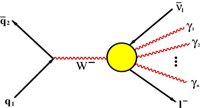
Figure 4: Production of a single $W^{-}$ in quark–antiquark collisions with multiphoton radiation in $W$-boson decay.

As was mentioned in the Introduction, the main purpose of this work is to provide a theoretical prediction for the multiphoton radiation in leptonic $W$-boson decays within the YFS exclusive exponentiation scheme. In this paper we consider the process of single-$W$ production in hadronic collisions at the parton level, i.e.

$$q_{1}(p_{1})+\bar{q}_{2}(p_{2})\longrightarrow W^{\pm}(Q)\longrightarrow l(q_{l})+\nu(q_{\nu})+\gamma(k_{1})+\ldots+\gamma(k_{n}),\>\>\>(n=0,1,\ldots),$$ (20)

depicted diagrammatically in Fig. 4. Here we do not rely on the small-lepton-mass approximation, i.e. the formulae below are given for arbitrary final-state lepton masses.

The ${\cal O}(\alpha)$ QED YFS-exponentiated total cross section for this process reads

$$\sigma^{tot}_{\rm YFS}=\sum_{n=0}^{\infty}\int\frac{d^{3}q_{l}}{q_{l}^{0}}\frac{d^{3}q_{\nu}}{q_{\nu}^{0}}\rho_{n}^{(1)}(p_{1},p_{2},q_{1},q_{2},k_{1},\ldots,k_{n}),$$ (21)

where

$$\rho_{n}^{(1)}=\,e^{Y(Q,q_{l};k_{s})}\,\frac{1}{n!} \prod_{i=1}^{n}\frac{d^{3}k_{i}}{k_{i}^{0}}\tilde{S}(Q,q_{l},k_{i})\theta(k_{i}^{0}-k_{s})\,\delta^{(4)}\left(p_{1}+p_{2}-q_{l}-q_{\nu}-\sum_{i=1}^{n}k_{i}\right)$$ (22)

$$\times\left[\,\bar{\beta}_{0}^{(1)}(p_{1},p_{2},q_{l},q_{\nu})+\sum_{i=1}^{n}\frac{\bar{\beta}_{1}^{(1)}(p_{1},p_{2},q_{l},q_{\nu},k_{i})}{\tilde{S}(Q,q_{l},k_{i})}\,\right];$$

here,

$$\tilde{S}(Q,q_{l},k)=-\frac{\alpha}{4\pi^{2}}\left(\frac{Q}{kQ}-\frac{q_{l}}{kq_{l}}\right)^{2}$$ (23)

is the soft-photon radiation (eikonal) factor and

$$Y(Q,q_{l};k_{s})=2\alpha\left[\Re B(Q,q_{l};m_{\gamma})+\tilde{B}(Q,q_{l};m_{\gamma},k_{s})\right]$$ (24)

the YFS form factor, where $B$ and $\tilde{B}$ are the virtual- and real-photon IR YFS functions, given explicitly in Appendix B for arbitrary four-momenta and masses of charged particles. These IR functions are regularized with the dummy photon mass $m_{\gamma}$, which cancels out in their sum. The real-photon function $\tilde{B}$ depends also on the soft-photon energy cut-off $k_{s}\ll E_{CM}$, which means that it was integrated analytically over the photons with energies $E_{\gamma}\leq k_{s}$. The photons with energies $E_{\gamma}>k_{s}$ are generated exclusively with the help of Monte Carlo techniques. The soft cut-off $k_{s}$ is a dummy parameter, i.e. the resulting cross section does not depend on it, which can be checked both analytically (e.g. by differentiating Eq. (22) over $k_{s}$) and numerically (by evaluating the cross section for different values of $k_{s}$). One of the advantages of exponentiation is that $k_{s}$ can be put arbitrarily low without causing any part of the cross section to become negative – in contrast to fixed-order calculations. In Eq. (22), $\bar{\beta}_{0}^{(1)}$ and $\bar{\beta}_{1}^{(1)}$ are the YFS non-IR functions, calculated perturbatively through ${\cal O}(\alpha)$. We present them below in the centre-of-mass (CM) frame of the incoming quarks, i.e. the rest frame of $W$, with the $+z$ axis pointing in the quark $q_{1}$ direction.

The function $\bar{\beta}_{0}^{(1)}$ is given by

$$\bar{\beta}_{0}^{(1)}(p_{1},p_{2},q_{l},q_{\nu})=\bar{\beta}_{0}^{(0)}(p_{1},p_{2},q_{l},q_{\nu})\left[\,1+\delta^{(1)}(Q,q_{l},q_{\nu})\,\right],$$ (25)

where $\bar{\beta}_{0}^{(0)}$ is related to the Born-level cross section through

$$\frac{1}{2}\bar{\beta}_{0}^{(0)}=\frac{1}{\sqrt{\lambda(1,m_{l}/M,m_{\nu}/M)}}\,\frac{d\sigma_{0}}{d\Omega_{l}}=\frac{1}{16s\,(2\pi)^{2}}\,\frac{1}{12}\sum\left|{\cal M}^{(0)}\right|^{2},$$ (26)

with $s=(q_{1}+q_{2})^{2}=Q^{2}$ and $\lambda(x,y,z)=x^{2}+y^{2}+z^{2}-2xy-2xz-2yz$. The factor $\frac{1}{12}=\frac{1}{4}\cdot\frac{1}{3}$ corresponds to averaging over the initial-state quark spins and colours (the colour contents has been extracted explicitly), and the sum $\sum$ runs over all the initial- and final-state spin indices. In Eq. (25), the correction

$$\delta^{(1)}(Q,q_{l},q_{\nu})=\delta^{v}_{\rm EW}(Q,q_{l},q_{\nu};m_{\gamma})-2\alpha\Re B(Q,q_{l};m_{\gamma})$$ (27)

is the 1st order non-IR correction to the $\bar{\beta}_{0}$ function, where $\delta^{v}_{\rm EW}$ is the ${\cal O}(\alpha)$ EW virtual correction. Since in this paper we limit ourselves to the QED-like corrections, from Eqs. (11) and (59) we have

$$\delta_{\rm QED}^{(1)}(Q,q_{l})=\frac{\alpha}{\pi}\left(\ln\frac{M}{m_{l}}+\frac{1}{2}\right).$$ (28)

Although Eqs. (11) and (59) were obtained in the small-lepton-mass approximation, $m_{l}\ll M$, we have checked that the above formula remains true for arbitrary lepton mass $m_{l}<M$ (of course, under the assumption that $\delta_{\rm QED}^{v}$ contains only the IR- and mass-singular terms).

The function $\bar{\beta}_{1}^{(1)}$ is the YFS non-IR function corresponding to the single-real-hard photon radiation. It is related to differential cross sections through

$$\frac{1}{2}\bar{\beta}_{1}^{(1)}(p_{1},p_{2},q_{l},q_{\nu},k)=\frac{1}{\sqrt{\Lambda(k)}}\,\frac{d\sigma_{1}}{d\Omega_{l}k^{0}dk^{0}d\Omega_{k}}-\tilde{S}(Q,q_{l},k)\,\frac{1}{\sqrt{\lambda}}\,\frac{d\sigma_{0}}{d\Omega_{l}},$$ (29)

where

$$\frac{d\sigma_{1}}{d\Omega_{l}k^{0}dk^{0}d\Omega_{k}}=\frac{\sqrt{\Lambda(k)}}{32s\,(2\pi)^{5}}\,\frac{1}{12}\sum\left|{\cal M}^{(1)}\right|^{2},$$ (30)

with

$$\sqrt{\Lambda(k)}=\frac{2\,|\vec{q}_{l}|^{2}}{|\vec{q}_{l}|(M-k^{0})+q_{l}^{0}|\vec{k}|\cos\theta_{lk}}$$ (31)

the phase-space factor (coming from the phase-space integration eliminating the energy-momentum conservation $\delta^{(4)}$-function for single-photon radiation), where $\theta_{lk}=\angle(\vec{q}_{l},\vec{k})$; in the soft-photon limit $\Lambda(k\rightarrow 0)\rightarrow\lambda$. The sum $\sum$ in Eq. (30) again runs over the initial- and final-state spin indices, this time inluding also those of the radiative photon. Thus, we finally have

$$\bar{\beta}_{1}^{(1)}(p_{1},p_{2},q_{l},q_{\nu},k)=\frac{1}{16s\,(2\pi)^{5}}\,\frac{1}{12}\sum\left|{\cal M}^{(1)}\right|^{2}-\tilde{S}(Q,q_{l},k)\bar{\beta}_{0}^{(0)}(p_{1},p_{2},q_{l},q_{\nu}).$$ (32)

There are several advantages in using the matrix elements of Section 2. Firstly, the respective spin amplitudes are derived without the assumption of the energy-momentum conservation. Therefore, they can be used directly in evaluations of the above YFS $\bar{\beta}$-functions over the multiphoton phase space, without the need to resort to any “reduction procedure”, which reduces the multiphoton phase space to the $0$-photon phase space for $\bar{\beta}_{0}$ and the $1$-photon phase space for $\bar{\beta}_{1}$, see e.g. [22, 34]. Secondly, since the spin amplitudes are obtained for massive fermions, there is no need to use any phase-space slicing or subtraction methods in order to separate mass singularities [17]. Using spin amplitudes instead of explicit analytical formulae for the squared matrix elements may also be useful for some dedicated studies, such as investigation of various $W$-polarization contributions, “new physics” searches (spin amplitudes can be easily modified to include some “new physics” components), etc. And, which is important in practice, the numerical evaluation of the matrix elements based on the above spin amplitudes is fast in terms of CPU time.

In computing the matrix element $\sum\left|{\cal M}^{(1)}\right|^{2}$ we observed a loss of numerical precision $\sim$ ${\cal O}(0.1\%$) when the angle between the radiative photon and the electron (positron), $\theta_{e\gamma}$, was $\sim$ ${\cal O}(10^{-6}$). It turned out that most of this precision loss was coming from huge numerical cancellations between the terms in the universal eikonal factor of Eq. (15) (the factor in front of the first $S$-function). We improved this by correcting the above matrix element according to

$$\sum\left|{\cal M}^{(1)}\right|^{2}\longrightarrow\sum\left|{\cal M}^{(1)}\right|^{2}+\delta_{coll},$$ (33)

where

$$\delta_{coll}=\left[\,16\pi^{3}\tilde{S}(Q,q_{l},k)-e^{2}\sum_{\kappa}\left|\frac{q_{l}\cdot\epsilon_{\gamma}^{\ast}(\kappa)}{k\cdot q_{l}}-\frac{Q\cdot\epsilon_{\gamma}^{\ast}(\kappa)}{k\cdot Q}\right|^{2}\,\right]\sum\left|{\cal M}^{(0)}\right|^{2}.$$ (34)

Algebraically, the two terms in the square brackets are identical. Numerically, however, they can differ for ultra-collinear photon radiation, owing to huge cancellations in the second term leading to a loss of numerical precision. Therefore, this correction effectively replaces the numerically unstable part of the matrix element $\sum\left|{\cal M}^{(1)}\right|^{2}$ corresponding to the second term in Eq. (34) with the numerically safe one corresponding to the first term, obtained directly from the particles four-momenta. We have checked that the above modification is sufficient for the numerical precision of ${\cal O}(10^{-4}$) for $\theta_{e\gamma}\lesssim 10^{-6}$ and of ${\cal O}(10^{-8}$) for the total cross section. By looking at Eq. (32) one can notice that the part of the matrix element $\sum\left|{\cal M}^{(1)}\right|^{2}$ that is proportional to the soft-photon factor $\tilde{S}$ exactly cancels in the calculation of the $\bar{\beta}_{1}^{(1)}$ function. We could, therefore, perform this cancellation algebraically and thus avoid the above numerical problems. We, however, keep this term in $\sum\left|{\cal M}^{(1)}\right|^{2}$ because apart from the YFS exponentiation we want to have in our program also the non-exponentiated, fixed-order ${\cal O}(\alpha)$ calculation. Since it is now calculated in the same way as the second term in Eq. (32), it exactly cancels numerically in the evaluation of the $\bar{\beta}_{1}^{(1)}$ function.

This completes our description of the cross section for process (20) with the ${\cal O}(\alpha)$ QED YFS exponentiation. In order to compute this cross section and generate events, we have developed an appropriate MC algorithm, which will be described in detail elsewhere [23]. We will complete this paper by presenting some results of numerical tests of the corresponding MC program, called WINHAC.

4 Numerical results

We performed several numerical tests of the MC event generator WINHAC, which implements the calculations presented above. Here we discuss some of the results. We considered the following process:

$$d+\bar{u}\longrightarrow W^{-}\longrightarrow l+\bar{\nu_{l}},$$ (35)

where $l=e,\,\mu,\,\tau$. We have checked that the results remain unchanged when we switch to the corresponding process of $W^{+}$ production and decay. Our MC calculations were done using the $G_{\mu}$ scheme and the fixed-width scheme. All the results below, unless stated otherwise, have been obtained for the following input parameters:

$$m_{d}=3\times 10^{-3}\,{\rm GeV},\>\>\>\>\>\>m_{u}=6\times 10^{-3},\>\>\>\>\>\>V_{ud}=1,\>\>\>\>\>\>m_{\nu_{l}}=0,$$ (36)

$$m_{e}=0.511\times 10^{-3}\,{\rm GeV},\>\>\>\>\>\>m_{\mu}=0.10565836\,{\rm GeV},\>\>\>\>\>\>m_{\tau}=1.77703\,{\rm GeV},$$

$$M_{W}=80.423\,{\rm GeV},\>\>\>\>\>\>M_{Z}=91.1882\,{\rm GeV}$$

$$s_{W}^{2}=1-\frac{M_{W}^{2}}{M_{Z}^{2}},\>\>\>\>\>\>\Gamma_{W}=\frac{3G_{\mu}M_{W}^{3}}{2\sqrt{2}\pi}\left(1+\frac{2\alpha_{s}}{3\pi}\right),$$

$$\alpha=137.03599976,\>\>\>\>\>\>G_{\mu}=1.16639\times 10^{-5}\,{\rm GeV}^{-2},\>\>\>\>\>\>\alpha_{s}=0.1185,$$

$$E_{CM}=\sqrt{s}=M_{W}.$$

4.1 General tests

We have performed several numerical tests of the MC event generator WINHAC aimed at checking the correctness of the implemented matrix elements as well as the corresponding MC algorithm.

In order to cross-check the matrix elements presented here, we implemented in our MC program the matrix elements of Ref. [18], which in the following we shall call B&K. These latter matrix elements were obtained in the small-lepton-mass approximation $m_{l}\ll M_{W}$; their precision therefore is of ${\cal O}(m_{l}^{2}/M_{W}^{2}$), which for electrons gives ${\cal O}(10^{-10}$). Since our spin amplitudes are obtained for massive fermions, we performed the comparisons of these matrix elements for electronic $W$-boson decays. We did this by taking the difference between the corresponding MC weights on an event-by-event basis and calculating the average of this difference over the whole MC sample. For both the Born-level and ${\cal O}(\alpha)$ matrix elements, we reached an agreement at the level of $\sim 10^{-8}$.

Then, we performed several tests to check the MC algorithm of the program WINHAC. An important test of the algorithm for MC integration and event generation according to Eq. (21) is to reproduce fixed-order calculations. The strict Born-level cross section can be obtained from Eq. (21) by truncating the perturbation series in $\alpha$ at the lowest-order term, which amounts to

$$\sigma_{0}^{tot}=\int\frac{d^{3}q_{l}}{q_{l}^{0}}\frac{d^{3}q_{\nu}}{q_{\nu}^{0}}\,\rho_{0}^{(0)}\,e^{-Y}\,.$$ (37)

Within the multiphoton MC algorithm, this means calculating an appropriate weight if the photon number $n=0$ and setting it to zero if $n>0$. The Born-level total cross section can be easily calculated analytically. In the small-fermion-mass approximation and in the fixed-width scheme it reads

$$\sigma_{0}^{tot}=\frac{\alpha_{G_{\mu}}^{2}\pi|V_{q_{1}q_{2}}|^{2}}{36s_{W}^{4}}\,\frac{s}{(s-M_{W}^{2})^{2}+M_{W}^{2}\Gamma_{W}^{2}}\,.$$ (38)

Calculation	$\sigma_{0}^{tot}$ [nb]
	$e$	$\mu$	$\tau$
Analytical	$8.8872\>\>\>\>\>\;$	$8.8872\>\>\>\>\>\;$	$8.8872\>\>\>\>\>\;$
WINHAC	$8.8869\,(2)$	$8.8873\,(2)$	$8.8808\,(2)$

Table 1: The results for the total Born-level cross section from the MC program WINHAC compared with the analytical calculation in the small-fermion-mass approximation. The numbers in parentheses are statistical errors for the last digits.

In Table 1 we compare the results for the total Born cross section for $e$, $\mu$ and $\tau$ in the final state, calculated with the MC program WINHAC with those obtained from the analytical formula of Eq. (38). We see a very good agreement between these two calculations for $e$ and $\mu$. For $\tau$ they differ by $\sim 0.1\%$, which can be explained by the $\tau$-mass effects (they are not negligible as in the case of $e$ and $\mu$).

In a similar way, the first-order cross section can be obtained from Eq. (21) by truncating the perturbative series at ${\cal O}(\alpha)$ beyond the Born level, i.e.

$$\sigma_{1}^{tot} =\int\frac{d^{3}q_{l}}{q_{l}^{0}}\frac{d^{3}q_{\nu}}{q_{\nu}^{0}}\,\delta^{(4)}(p_{1}+p_{2}-q_{l}-q_{\nu})\,\bar{\beta}_{0}^{(0)}\left[\,1+\delta_{\rm QED}^{(1)}+Y\,\right]$$ (39)

$$+\int\frac{d^{3}q_{l}}{q_{l}^{0}}\frac{d^{3}q_{\nu}}{q_{\nu}^{0}}\frac{d^{3}k}{k^{0}}\,\delta^{(4)}(p_{1}+p_{2}-q_{l}-q_{\nu}-k)\left[\,\bar{\beta}_{1}^{(1)}+\tilde{S}\bar{\beta}_{0}^{(0)}\,\right]\theta(k^{0}-k_{s})\,,$$

where the first term on the r.h.s. corresponds to the Born plus virtual and real-soft-photon contribution, and the second term to the real-hard-photon contribution. In practice, this means that the first term is evaluated within the multiphoton algorithm only for $n=0$, the second only for $n=1$, otherwise the appropriate MC weights are set to zero.

Calculation	$\delta_{1}=\sigma_{1}^{tot}/\sigma_{0}^{tot}-1$
	$e$	$\mu$	$\tau$
WINHAC	$-1.5\,(3)\times 10^{-4}$	$-2.2\,(3)\times 10^{-4}$	$-0.3\,(2)\times 10^{-4}$

Table 2: The results for the ${\cal O}(\alpha)$ QED-like correction to the total cross section from the MC program WINHAC. The numbers in parentheses are statistical errors for the last digits.

In Table 2 we show the results from the program WINHAC for the pure ${\cal O}(\alpha)$ QED-like correction to the total cross section. As can be seen, the results for $e$ and $\mu$ are in good agreement with the numerical value of total QED-like correction to the $W$-boson width as given in Eq. (13). For $\tau$ we observe the difference of $\sim 1.5\times 10^{-4}$, which again can be explained by the $\tau$-mass effects.

$k_{0}$	$e$		$\mu$
	WINHAC	B&K	WINHAC	B&K
$0.01$	$19.69\,(3)$	$19.7$	$10.11\,(2)$	$10.1$
$0.05$	$11.61\,(2)$	$11.6$	$5.92\,(1)$	$5.9$
$0.10$	$8.31\,(2)$	$8.3$	$4.22\,(1)$	$4.2$
$0.15$	$6.47\,(2)$	$6.5$	$3.27\,(1)$	$3.3$
$0.20$	$5.23\,(1)$	$5.2$	$2.63\,(1)$	$2.6$
$0.30$	$3.61\,(1)$	$3.6$	$1.80\,(1)$	$1.8$
$0.40$	$2.57\,(1)$	$2.6$	$1.27\,(1)$	$1.3$
$0.50$	$1.84\,(1)$	$1.8$	$0.91\,(1)$	$0.9$
$0.60$	$1.29\,(1)$	$1.3$	$0.63\,(1)$	$0.6$
$0.70$	$0.86\,(1)$	$0.9$	$0.42\,(1)$	$0.4$
$0.80$	$0.52\,(1)$	$0.5$	$0.25\,(1)$	$0.2$
$0.90$	$0.24\,(1)$	$0.2$	$0.11\,(1)$	$0.1$

Table 3: The fraction of events (in %) with a photon energy greater than $k_{0}$ at ${\cal O}(\alpha)$ from the MC program WINHAC and from the MC program of Berends & Kleiss [18] (denoted as B&K) for $E_{CM}=90\,$GeV. The numbers in parentheses are statistical errors for the last digits.

In Table 3 we compare the results for the ${\cal O}(\alpha)$ hard-photon correction as a function of the lower photon-energy cut-off $k_{0}$, i.e.

$$\delta_{1}^{h}(k_{0})=\frac{1}{\sigma_{1}^{tot}}\int_{k_{0}}dE_{\gamma}\,\frac{d\sigma_{1}}{E_{\gamma}}\;\times 100\%\,,$$ (40)

for the centre-of-mass energy $E_{CM}=90\,$GeV, obtained from the program WINHAC and from the B&K MC program [18]. The results of these two programs agree very well within the statistical errors.

As the above fixed-order results from WINHAC have been obtained in the framework of the YFS-type multiphoton algorithm, they make us strongly confident in the correctness of the corresponding MC algorithm.

Calculation	$\sigma^{tot}\,$[nb]
	$e$	$\mu$	$\tau$
Fixed ${\cal O}(\alpha)$-level	$8.88564\,(14)$	$8.88539\,(12)$	$8.88047\,(10)$
YFS exponentiation	$8.88390\>\>\>(6)$	$8.88443\>\>\>(9)$	$8.87859\>\>\>(9)$
$\delta_{exp}=(\sigma_{\rm YFS}^{tot}-\sigma_{1}^{tot})/\sigma_{0}^{tot}$	$-2.0\,(1)\times 10^{-4}$	$-1.1\,(1)\times 10^{-4}$	$-2.1\,(0)\times 10^{-4}$

Table 4: The results for the fixed-${\cal O}(\alpha)$ and the YFS-exponentiated total cross section from the MC program WINHAC. The numbers in parentheses are statistical errors for the last digits.

In Table 4 we give the results for the total cross section at the fixed ${\cal O}(\alpha)$-level and including the YFS exponentiation as given in Eq. (21). The YFS-exponentiation corrections beyond ${\cal O}(\alpha)$ are $\sim 10^{-4}$, i.e. of the expected size of higher-order corrections.

4.2 Distributions

Figure 5: Distributions of the charged-lepton energy for BARE and CALO acceptances.

Figure 6: Distributions of the hardest-photon energy for BARE and CALO acceptances.

Figure 7: Distributions of the cosine of the hardest-photon polar angle for BARE and CALO acceptances.

Here we presents the results from WINHAC for some distributions at the Born level, with ${\cal O}(\alpha)$ QED-like corrections and including the YFS exponentiation. These results are given for two kinds of event selection: BARE – where the corresponding observables are obtained from bare-lepton four-momenta and no cuts are applied, and CALO – where the photon four-momenta are combined with the charged-lepton four-momenta if the opening angle between their directions $\angle(\vec{q}_{l},\vec{k})\leq 5^{\circ}$; such photons are discarded. No extra cuts are applied. The BARE acceptance is closer to experimental event selections for muons, while the CALO is closer to the ones for electrons. We, however, use them for both types of final states.

In Fig. 5 we present the distributions of the electron and muon energy for the fixed ${\cal O}(\alpha)$ corrections and for the YFS exponentiation. The upper plots show the absolute distributions for the BARE and CALO acceptances, respectively, while the lower plots show the relative differences between these two calculations, also for the BARE and CALO acceptances. At the Born level, the charged-lepton energy is fixed at $E_{l}\approx\frac{1}{2}\sqrt{s}$; therefore, the energy tails for $E_{l}<\frac{1}{2}\sqrt{s}$ in the above plots are the result of the real-photon radiation in $W$-boson decay. The YFS-exponentiation corrections beyond the fixed ${\cal O}(\alpha)$-level are large for the BARE acceptance: up to $\sim 15\%$ for electrons and up to $\sim 8\%$ for muons – they differ for these two decay channels. For the CALO acceptance these corrections are smaller, up to $\sim 4\%$, and they are almost identical for electrons and muons. This is because in this case the large corrections due to lepton-mass-log terms have been excluded by the photon–lepton recombination. As can be seen, the largest (negative) corrections are in the first radiative bin (i.e. the second highest one in the upper plots) and they change sign for low lepton energies.

In Fig. 6 we show the distributions of the hardest photon energy for the electron and muon $W$-decay channels. The notation is similar to that in Fig. 5. Again, for the BARE acceptance the YFS-exponentiation corrections beyond the fixed ${\cal O}(\alpha)$-level are large and different for these two channels: up to $\sim 15\%$ for electrons and up to $\sim 7\%$ for muons. For CALO they are smaller, $\sim 4\%$, and similar in the two channels. The corrections are largest for soft photons and decrease with the photon energy.

Finally, in Fig. 7 we show the distributions of the cosine of the hardest photon polar angle with respect to the incoming quark direction; the notation is as in Fig. 6. For the BARE acceptance the YFS-exponentiation corrections beyond the fixed ${\cal O}(\alpha)$-level are large and almost constant: $\sim 28\%$ for electrons and $\sim 14\%$ for muons. For CALO they are smaller, $6$–$7\%$, and similar in the electron and muon channels.

As can be seen from Figs. 5–7, the YFS exponentiation affects sizeably radiative events. All the above distributions have been obtained for the parton-level $W$-boson production at fixed CMS energy. In the actual proton–(anti)proton collisions the parton–parton CMS energy can change, which leads to an enhancement of the FSR corrections, in particular those due to the YFS exponentiation. This will be investigated elsewhere [35].

5 Summary and outlook

In this paper we have presented the calculations of the YFS QED exponentiation in leptonic $W$-boson decays. We have provided the fully massive spin amplitudes for the single $W$-boson production and decay, including the single-real-photon radiation in $W$ decays. We have obtained the numerically stable representations of the YFS form factor for the charged-particle decay. All this has been applied to the process of Drell–Yan-like $W$-boson production in hadronic collisions and implemented, at the parton level, in the Monte Carlo event generator WINHAC 1.0. For this purpose, an efficient multiphoton MC algorithm has been developed. The above spin amplitudes have been cross-checked with the independent analytical representations of the appropriate matrix elements [18] and they have been found to be in very good numerical agreement. We have also performed several numerical tests of the implemented MC algorithm. The results of these tests make us confident in the correctness of this MC algorithm.

Numerically, the YFS-exponentiation corrections beyond the fixed ${\cal O}(\alpha)$ calculations are at the level of $\sim 10^{-4}$ for the total cross section, which is the result of the KLN-theorem. However, for some distributions they can amount to between a few and over $20$ per cent. These corrections can be significantly reduced when a calorimetric-like recombination of radiative photons and charged leptons is applied. Such a treatment is experimentally natural for the electrons in the final state, but less obvious for the muons.

Here we presented the calculations for the QED-like corrections in the leptonic $W$-boson decays and for the parton-level $W$-production process only. We are planning to extend this, in the future, to the full proton–(anti)proton collisions and to include other ${\cal O}(\alpha)$ electroweak corrections. The next step would be the inclusion of the NLO QCD effects as well as soft-gluon resummation corrections. We are also going to perform further tests of the program WINHAC at the ${\cal O}(\alpha)$ and beyond, particularly comparisons with independent calculations for various observables. Last, but not least, the full documentation of the MC program WINHAC [23] is in preparation (to be submitted to Computer Physics Communications). There, the details of the corresponding MC algorithm will be given.

In this paper, we applied the QED YFS exponentiation in leptonic $W$-boson decays to the single-$W$ production process at hadron colliders. However, it can also be used to describe the photon radiation in $W$ decays in the processes of $W$-pair production at both hadron and electron–positron colliders. In particular, it can be rather easily implemented in our MC event generator YFSWW [21] for $W^{+}W^{-}$ production in $e^{+}e^{-}$ collisions, which will be necessary for the future linear colliders [3].

Acknowledgements

We would like to thank D. Bardin and B.F.L. Ward for useful discussions. We acknowledge the kind support of the CERN TH and EP Divisions.

Appendix A Spinorial string functions

Here we provide explicit formulae for the spinorial string functions introduced in Section 2. The general such function in the two-component Weyl-spinor basis reads [24]

$$S(p_{i},a_{1},\ldots,a_{n},p_{j})_{\sigma_{i}\sigma_{j}}^{\alpha}=\chi_{\sigma_{i}}^{\dagger}(p_{i})\left[a_{1},\ldots,a_{n}\right]^{\alpha}\chi_{\sigma_{j}}(p_{j}),$$ (41)

where

$$\chi_{+}(p)=\frac{1}{\sqrt{2|\vec{p}|(|\vec{p}|+p^{3})}}\genfrac{[}{]}{0.0pt}{}{|\vec{p}|+p^{3}}{p^{1}+ip^{2}},\>\>\>\>\>\>\>\chi_{-}(p)=\frac{1}{\sqrt{2|\vec{p}|(|\vec{p}|+p^{3})}}\genfrac{[}{]}{0.0pt}{}{-p^{1}+ip^{2}}{|\vec{p}|+p^{3}}$$ (42)

are the two-component Pauli spinors corresponding to an external fermion with four-momentum $p=(p^{0},\vec{p})=(p^{0},p^{1},p^{2},p^{3})$; for $p^{3}=-|\vec{p}|$ we choose

$$\chi_{+}(p)=\genfrac{[}{]}{0.0pt}{}{0}{1},\>\>\>\>\>\>\>\chi_{-}(p)=\genfrac{[}{]}{0.0pt}{}{-1}{\>\>\>0}.$$ (43)

The internal part of the above string function

$$\left[a_{1},\ldots,a_{n}\right]^{\alpha}=(\hbox to0.0pt{/\hss}a_{1})_{\alpha}(\hbox to0.0pt{/\hss}a_{2})_{-\alpha}\ldots(\hbox to0.0pt{/\hss}a_{n})_{(-1)^{n+1}\alpha}$$ (44)

is the product of 2$\times$2 $c$-number matrices, where

$$(\hbox to0.0pt{/\hss}a)_{\pm}=\left[\begin{array}[]{cc}a^{0}\mp a^{3}&\mp(a^{1}-ia^{2})\\ \mp(a^{1}-ia^{2})&a^{0}\pm a^{3}\\ \end{array}\right]$$ (45)

with $a=(a^{0},a^{1},a^{2},a^{3})$ the four-vector in the Minkowski space.

As can be seen, the spinorial function $S$ can be easily evaluated numerically for arbitrary $n$. One can just compute a product of internal 2$\times$2 matrices $(\hbox to0.0pt{/\hss}a_{i})_{\alpha}$, and then multiply the resulting matrix by the external 2-dimensional $c$-number vectors $\chi$. However, the numerical evaluation is more efficient if, instead of matrix-by-matrix multiplication, one performs matrix-by-vector multiplication. In our computation of the function $S$, we start from multiplying the left-hand-side vector $\chi^{\dagger}$ by the matrix $(\hbox to0.0pt{/\hss}a_{1})_{\alpha}$, and continue by multiplying the resulting vectors by the consecutive matrices $(\hbox to0.0pt{/\hss}a_{i})_{\alpha}$ until we reach the last matrix, $(\hbox to0.0pt{/\hss}a_{n})_{\alpha}$. The computation is completed by performing the scalar product of the final vector of the above multiplication with the right-hand-side vector $\chi$.

Three polarization vectors of a massive vector-boson with four-momentum $k=(k^{0},\vec{k})=(k^{0},k^{1},k^{2},k^{3})$ and the mass $m$ are, in the Cartesian basis, given by

$$\epsilon^{\mu}(k,\lambda=1) =\frac{1}{|\vec{k}|k_{T}}\,\left(0,k^{1}k^{3},k^{2}k^{3},-k_{T}^{2}\right),$$ (46)

$$\epsilon^{\mu}(k,\lambda=2) =\frac{1}{k_{T}}\,\left(0,-k^{2},k^{1},0\right),$$

$$\epsilon^{\mu}(k,\lambda=3) =\frac{k^{0}}{m|\vec{k}|}\,\left(\frac{|\vec{k}|^{2}}{k^{0}},k^{1},k^{2},k^{3}\right),$$

where $k_{T}=\sqrt{(k^{1})^{2}+(k^{2})^{2}}$ is the transverse momentum. For massless vector bosons, such as photons, $\epsilon^{\mu}(\lambda=3)=0$, i.e. there are only two non-zero polarizations $\epsilon^{\mu}(\lambda=1)$ and $\epsilon^{\mu}(\lambda=2)$. Helicity eigenstates can be obtained from the above polarization vectors through

$$\epsilon_{hel}(k,\lambda=\pm) =\frac{1}{\sqrt{2}}\,\left[\,\mp\epsilon(k,\lambda=1)-i\epsilon(k,\lambda=2)\,\right]\,,$$ (47)

$$\epsilon_{hel}(k,\lambda=0) =\epsilon(k,\lambda=3).$$

Appendix B The YFS IR functions

In Ref. [36] we provided the general formulae for the YFS IR functions $\Re B$ and $\tilde{B}$ for a pair of charged particles of arbitrary masses and four-momenta. This representation works very well for particle production or scattering processes; however, it becomes numerically unstable for charged-particle decays. Therefore, for the process

$$W^{\pm}(Q)\longrightarrow l^{\pm}(q)+\overset{(-)}{\nu_{l}}(q^{\prime}),$$ (48)

we have to obtain different representations for these functions. A specific feature of the above process is that a QED-radiation dipole is stretched between a decaying particle ($W$) and a decay product ($l$). For such a dipole, a four-momentum transfer between its constituents is non-negative:

$$t=(Q-q)^{2}\geq 0,$$ (49)

in contrast to scattering processes. In such a case, the corresponding IR integrals have to be calculated in a slightly different way than was done in Ref. [36] for $t<0$. Special care is also needed for the limiting case $t=0$, which occurs for the two-body $W$-boson leptonic decay when the neutrino mass is neglected. For the sake of numerical stability, it has to be treated separately.

The YFS virtual- and real-photon IR functions for a pair of charged particles with the four-momenta $(Q,\,q)$ are defined as follows [22]

$$B(Q,q;m_{\gamma}) =\frac{i}{8\pi^{3}}\int\frac{d^{4}k}{k^{2}-m_{\gamma}^{2}+i\varepsilon}\left(\frac{2q-k}{k^{2}-2kq+i\varepsilon}-\frac{2Q-k}{k^{2}-2kQ+i\varepsilon}\right)^{2},$$ (50)

$$\tilde{B}(Q,q;m_{\gamma},k_{s}) =-\frac{1}{8\pi^{2}}\int_{k^{0}<k_{s}}\frac{d^{3}k}{k^{0}}\left(\frac{q}{kq}-\frac{Q}{kQ}\right)^{2},$$ (51)

where $m_{\gamma}$ is a dummy photon mass used to regularize the IR-divergent integrals ($m_{\gamma}\ll k_{s}$), while $k_{s}$ is the soft-photon cut-off, up to which the integration over the real-photon four-momenta is carried over analytically ($k_{s}\ll Q^{0}$). The explicit analytical formulae for these functions are presented below.

B.1 The virtual-photon IR function

The virtual-photon IR function reads as follows:

I.

$t=(Q-q)^{2}>0$:

$$2\alpha\Re B(Q,q;m_{\gamma})=\frac{\alpha}{\pi}\left\{\left[\,\nu A(Q,q)-1\,\right]\,\ln\frac{m_{\gamma}^{2}}{Mm}+\frac{1}{2}A_{1}(Q,q)-\nu A_{3}(Q,q)\right\},$$ (52)

with

$$A(Q,q) =\frac{1}{\lambda}\ln\frac{\lambda+\nu}{Mm},$$ (53)

$$A_{1}(Q,q) =\frac{M^{2}-m^{2}}{t}\ln\frac{M}{m}-\frac{2\lambda^{2}}{t}\,A(Q,q)-2,$$ (54)

$$A_{3}(Q,q) =A(Q,q)\,\ln\frac{2\lambda}{Mm}+\frac{1}{\lambda}\bigg{[}\frac{1}{4}\left(\ln\frac{\lambda+\nu}{M^{2}}+2\ln\frac{\lambda-\nu+M^{2}}{t}\right)\ln\frac{\lambda+\nu}{M^{2}}$$

$$+\frac{1}{4}\left(\ln\frac{\lambda+\nu}{m^{2}}-2\ln\frac{\lambda+\nu-m^{2}}{m^{2}}\right)\ln\frac{\lambda+\nu}{m^{2}}$$

$$+\frac{1}{2}\ln\eta\ln(1+\eta)-\frac{1}{2}\ln\zeta\ln(1+\zeta)+\Re\mathrm{Li}_{2}(-\eta)-\Re\mathrm{Li}_{2}(-\zeta)\bigg{]},$$ (55)

where

$$\nu=Qq,\>\>\>\>\lambda=\sqrt{(\nu-Mm)(\nu+Mm)},\>\>\>\>Q^{2}=M^{2},\>\>q^{2}=m^{2},\>\>M>m\,,$$ (56)

$$t=M^{2}+m^{2}-2\nu,\>\>\>\>\>\>\>\>Mm\leq\nu<\frac{1}{2}\left(M^{2}+m^{2}\right)\,,$$

$$\eta=\frac{m^{2}t}{2\lambda(2\lambda+\nu-m^{2})},\>\>\>\>\>\>\>\>\zeta=\frac{\lambda+\nu}{m^{2}}\,\eta\,,$$

and

$$\mathrm{Li}_{2}(y)=-\int_{0}^{y}\frac{dx}{x}\ln(1-x),\>\>\>\>\>\>\>\>|\arg(1-y)|<\pi,$$ (57)

is the Spence dilogarithm function.

II.

$t=(Q-q)^{2}=0$:

$$2\alpha\Re B(Q,q;m_{\gamma})=\frac{\alpha}{\pi}\left\{\left(\frac{M^{2}+m^{2}}{M^{2}-m^{2}}\ln\frac{M}{m}-1\right)\left(\ln\frac{m_{\gamma}^{2}}{Mm}+\frac{1}{2}\right)\right\}\,.$$ (58)

In the limit $m\ll M$ we get

$$2\alpha\Re B(Q,q;m_{\gamma})\underset{m\ll M}{=}\frac{\alpha}{\pi}\left\{2\left(\ln\frac{M}{m}-1\right)\ln\frac{m_{\gamma}}{M}+\ln^{2}\frac{M}{m}-\frac{1}{2}\ln\frac{M}{m}-\frac{1}{2}\right\}\,.$$ (59)

B.2 The real-photon IR function

For the real-photon IR function we obtain

I.

$t=(Q-q)^{2}>0$:

$$\tilde{B}(Q,q;m_{\gamma},k_{s})=\frac{\alpha}{\pi}\,\bigg{\{} \left[\,\nu A(Q,q)-1\,\right]\,\ln\frac{4k_{s}^{2}}{m_{\gamma}^{2}}-\frac{M^{2}}{2}A_{4}(Q,Q)-\frac{m^{2}}{2}A_{4}(q,q)$$ (60)

$$-\nu A_{4}(Q,q)\bigg{\}},$$

with

$$A_{4}(p,p) =\frac{1}{p^{2}\beta}\ln\frac{1-\beta}{1+\beta},\>\>\>\>\>\>\>\>\beta=\frac{|\vec{p}|}{p^{0}},$$ (61)

$$A_{4}(Q,q) =\frac{1}{\kappa}\left\{\ln\left|\frac{V^{2}}{t}\right|\sum_{i=0}^{1}(-1)^{n+1}\left[\,X(z_{i};y_{1},y_{4},y_{2},y_{3})+R(z_{i})\,\right]\right\}\,,$$ (62)

where

$$R(z)=Y_{14}(z)+Y_{21}(z)+Y_{32}(z)-Y_{34}(z)$$ (63)

$$\hskip 28.45274pt+\frac{1}{2}X(z;y_{1},y_{2},y_{3},y_{4})X(z;y_{2},y_{3},y_{1},y_{4})\,,$$

$$Y_{ij}(z)=2Z_{ij}(z)+\frac{1}{2}\ln^{2}\left|\frac{z-y_{i}}{z-y_{j}}\right|\,,$$

$$Z_{ij}(z)=\Re\mathrm{Li}_{2}\left(\frac{y_{j}-y_{i}}{z-y_{i}}\right)\,,$$

$$X(z;a,b,c,d)=\ln\left|\frac{(z-a)(z-b)}{(z-c)(z-d)}\right|\,,$$

and

$$z_{0}=\frac{|\vec{q}|}{T}\,,\hskip 139.4185ptz_{1}=\frac{|\vec{Q}|}{T}-1\,;$$ (64)

$$y_{1}=-\frac{1}{2T}\left[\,T+\Omega-\frac{\omega\delta+\kappa}{t}\,V\,\right],\hskip 14.22636pty_{2}=y_{1}-\frac{\kappa V}{tT}\,,$$

$$y_{3}=-\frac{1}{2T}\left[\,T-\Omega+\frac{\omega\delta+\kappa}{V}\,\right],\hskip 25.60747pty_{4}=y_{3}+\frac{\kappa}{TV}\,;$$

$$\kappa=\sqrt{(\omega^{2}-t)(\delta^{2}-t)}\,,\hskip 14.22636pt\delta=M-m,\>\>\omega=M+m\,,$$

$$T=\sqrt{\Delta^{2}-t}\,,\>\>V=\Delta+T,\hskip 14.22636pt\Delta=Q^{0}-q^{0},\>\>\Omega=Q^{0}+q^{0}\,,$$

while $\nu$ and $A(Q,q)$ are as given in the previous subsection. We have checked that this analytical representation is numerically stable for $t\gtrsim 10^{-10}\,\mathrm{GeV}^{2}$, when computed in any Lorentz frame, which is neither $W$ nor $l$ rest frame. In these frames we need an explicit analytical formula for $A_{4}(p,p)$ in the limit $\beta\rightarrow 0$. It reads

$$A_{4}(p,p)\underset{p=(m,\vec{0})}{=}-\frac{2}{m^{2}}\,.$$ (65)

In the $W$ rest frame, i.e. for $Q=(M,\vec{0})$, the function $A_{4}(Q,q)$ can be simplified to get

$$A_{4}(Q,q){=}\frac{1}{2M\bar{q}}\bigg{[} \ln\frac{M-E+\bar{q}}{M-E-\bar{q}}\ln\frac{E+\bar{q}}{M}-2\ln\frac{2\bar{q}(M-E+\bar{q})}{Mm}\ln\frac{E+\bar{q}}{M}$$ (66)

$$+ 2\Re\mathrm{Li}_{2}\left(\frac{E-\bar{q}}{M}\right)-2\Re\mathrm{Li}_{2}\left(\frac{E+\bar{q}}{M}\right)$$

$$+ \Re\mathrm{Li}_{2}\left(\frac{M-E-\bar{q}}{-2\bar{q}}\right)-\Re\mathrm{Li}_{2}\left(\frac{M-E+\bar{q}}{2\bar{q}}\right)$$

$$+ \Re\mathrm{Li}_{2}\left(\frac{M(E+\bar{q})-m^{2}}{2M\bar{q}}\right)-\Re\mathrm{Li}_{2}\left(\frac{M(E-\bar{q})-m^{2}}{-2M\bar{q}}\right)\,\bigg{]}\,,$$

where $E=q^{0},\,\bar{q}=|\vec{q}|$.

I.

$t=(Q-q)^{2}=0$:

For $t=0$ the functions $A(Q,q),A_{4}(Q,Q),A_{4}(q,q)$ can remain the same as for $t>0$, but we need a new, numerically stable, representation for the function $A_{4}(Q,q)$. It can be cast in the form

$$A_{4}(Q,q)=\frac{1}{\mu^{2}}\left[\,\ln\frac{2\Delta^{2}}{\mu^{2}}\ln\left|\frac{\xi_{2}\xi_{3}}{\xi_{1}}\right|+U(z_{1})-U(z_{0})\right]\,,$$ (67)

where

$$U(z)=\frac{1}{2}\ln^{2}\left|\frac{(z-y_{1})(z-y_{2})}{z-y_{3}}\right|+\ln|z-y_{1}|\ln\frac{|z-y_{1}|}{(z-y_{2})^{2}}$$ (68)

$$\hskip 28.45274pt+2\Re\mathrm{Li}_{2}\left(\frac{y_{2}-y_{1}}{z-y_{1}}\right)+2\Re\mathrm{Li}_{2}\left(\frac{y_{3}-y_{2}}{z-y_{2}}\right)\,;$$

$$\xi_{i}=\frac{z_{0}-y_{i}}{z_{1}-y_{i}}\,,\hskip 14.22636ptz_{0}=\frac{|\vec{q}|}{\Delta}\,,\>\>\>\>z_{1}=\frac{|\vec{Q}|}{\Delta}-1\,;$$

$$y_{1}=\frac{q^{0}}{\Delta}\,,\>\>\>\>y_{2}=y_{1}-\frac{\mu^{2}}{2\Delta^{2}}\,,\>\>\>\>y_{3}=-y_{1}+\frac{2m^{2}}{\mu^{2}}\,;$$

$$\Delta=Q^{0}-q^{0}\,,\>\>\>\>\mu^{2}=M^{2}-m^{2}\,.$$

In the $W$ rest frame we get

$$A_{4}(Q,q)\underset{Q=(M,\vec{0})}{=}-\frac{2}{M^{2}-m^{2}}\left[\,\ln^{2}\frac{M}{m}+\mathrm{Li}_{2}\left(\frac{M^{2}-m^{2}}{M^{2}}\right)\,\right]\,.$$ (69)

Then, in the small-lepton-mass limit, $m\ll M$, we obtain a simple expression for the function $\tilde{B}$ in the $W$ rest frame:

$$2\alpha\tilde{B}(Q,q;m_{\gamma},k_{s})\underset{m\ll M}{=}\frac{\alpha}{\pi}\left\{2\left(\ln\frac{M}{m}-1\right)\ln\frac{2k_{s}}{m_{\gamma}}-\ln^{2}\frac{M}{m}+\ln\frac{M}{m}+1-\frac{\pi^{2}}{6}\right\}.$$ (70)

After combining this with the virtual-photon function of Eq. (59), we obtain a simple expression for the YFS form factor in the $W$ rest frame:

$$Y(Q,q;k_{s})\underset{m\ll M}{=}\frac{\alpha}{\pi}\left\{2\left(\ln\frac{M}{m}-1\right)\ln\frac{2k_{s}}{M}+\frac{1}{2}\ln\frac{M}{m}-\frac{1}{2}-\frac{\pi^{2}}{6}\right\}.$$ (71)

As can be seen see explicitly, it is free of the IR singularity as well as of the Sudakov double-logarithms.

References

- [1] G. Altarelli, T. Sjöstrand, and F. Zwirner, editors, Physics at LEP2 (CERN 96-01, Geneva, 1996), 2 vols.
- [2] S. Jadach, G. Passarino, and R. Pittau, editors, Reports of the Working Groups on Precision Calculations for LEP2 Physics (CERN 2000-009, Geneva, 2000).
- [3] ECFA/DESY LC Physics Working Group, J. A. Aguilar-Saavedra et al., TESLA Technical Design Report Part III: Physics at an Linear Collider, SLAC-REPRINT-2001-002, DESY-01-011, DESY-2001-011, DESY-01-011C, DESY-2001-011C, DESY-TESLA-2001-23, DESY-TESLA-FEL-2001-05, ECFA-2001-209, Mar. 2001, hep-ph/0106315.
- [4] G. Altarelli and M. Mangano, editors, Proceedings of the Workshop on Standard Model Physics (and More) at the LHC (CERN 2000-004, Geneva, 2000).
- [5] M. Dittmar, F. Pauss, and D. Zurcher, Phys. Rev. D56, 7284 (1997), hep-ex/9705004.
- [6] W. Beenakker, F. A. Berends, and A. P. Chapovsky, Phys. Lett. B435, 233 (1998), hep-ph/9805327.
- [7] S. Jadach, W. Płaczek, M. Skrzypek, B. F. L. Ward, and Z. Wa̧s, Phys. Rev. D61, 113010 (2000).
- [8] U. Baur, S. Keller, and D. Wackeroth, Phys. Rev. D59, 013002 (1998).
- [9] W. J. Marciano and A. Sirlin, Phys. Rev. D8, 3612 (1973).
- [10] J. Fleischer and F. Jegerlehner, Z. Phys. C26, 629 (1985).
- [11] D. Bardin, S. Riemann, and T. Riemann, Z. Phys. C32, 121 (1986).
- [12] A. Denner and T. Sack, Z. Phys. C46, 653 (1990).
- [13] W. Beenakker, F. A. Berends, and A. P. Chapovsky, Nucl. Phys. B548, 3 (1999), hep-ph/9811481.
- [14] A. Denner, S. Dittmaier, M. Roth, and D. Wackeroth, Nucl. Phys. B587, 67 (2000), hep-ph/0006307.
- [15] D. Wackeroth and W. Hollik, Phys. Rev. D55, 6788 (1997).
- [16] V. A. Zykunov, Lowest order electroweak radiative corrections to the single production in polarized hadron hadron collisions, High energy physics and quantum field theory, Tver (2000), p. 399, hep-ph/0107059.
- [17] S. Dittmaier and M. Krämer, Phys. Rev. D65, 073007 (2002), hep-ph/0109062.
- [18] F. Berends and R. Kleiss, Z. Phys. C27, 365 (1985).
- [19] U. Baur and T. Stelzer, Phys. Rev. D61, 073007 (2000), hep-ph/9910206.
- [20] E. Barberio, B. van Eijk, and Z. Wa̧s, Comput. Phys. Commun. 66, 115 (1991), ibid. 79, 291 (1994).
- [21] S. Jadach, W. Płaczek, M. Skrzypek, B. F. L. Ward, and Z. Wa̧s, Comput. Phys. Commun. 140, 432 (2001), hep-ph/0103163.
- [22] D. R. Yennie, S. Frautschi, and H. Suura, Ann. Phys. (NY) 13, 379 (1961).
- [23] S. Jadach and W. Płaczek, WINHAC 1.00: The Monte Carlo Event Generator for Single -Boson Production with Leptonic Decays in Hadron Collisions, available from the authors; documentation in preparation.
- [24] K. Hagiwara and D. Zeppenfeld, Nucl. Phys. B274, 1 (1986).
- [25] D. Y. Bardin, A. Leike, T. Riemann, and M. Sachwitz, Phys. Lett. B206, 539 (1988).
- [26] S. Haywood et al., Electroweak Physics, in [4].
- [27] J. Fleischer, F. Jegerlehner, and M. Zrałek, Z. Phys. C42, 409 (1989).
- [28] T. Kinoshita, J. Math. Phys. 3, 650 (1962).
- [29] T. D. Lee and M. Nauenberg, Phys. Rev. B133, 1549 (1964).
- [30] U. Baur and D. Zeppenfeld, Phys. Rev. Lett. 75, 1002 (1995).
- [31] E. Argyres et al., Phys. Lett. B358, 339 (1995).
- [32] M. Passera and A. Sirlin, Phys. Rev. D58, 113010 (1998), hep-ph/9804309.
- [33] A. Sirlin, Recent developments in the study of unstable particle processes, Proceedings of the IVth International Symposium on Radiative Corrections (RADCOR 98): “Applications of Quantum Field Theory to Phenomenology”, Barcelona, 1998, ed. by J. Sola (World Scientific, Singapore, 1999), p. 546, hep-ph/9811467.
- [34] S. Jadach and B. F. L. Ward, Comput. Phys. Commun. 56, 351 (1990).
- [35] W. Płaczek and S. Jadach, in preparation.
- [36] S. Jadach, W. Płaczek, M. Skrzypek, and B. F. L. Ward, Phys. Rev. D54, 5434 (1996).