Abstract

An investigation of the $s$-wave channels in meson-meson scattering is performed within a $U(3)$ chiral unitary approach. Our calculations are based on a chiral effective Lagrangian which includes the $\eta^{\prime}$ as an explicit degree of freedom and incorporates important features of the underlying QCD Lagrangian such as the axial $U(1)$ anomaly. We employ a coupled channel Bethe-Salpeter equation to generate poles from composed states of two pseudoscalar mesons. Our results are compared with experimental phase shifts up to $1.5\,\mathrm{GeV}$ and effects of the $\eta^{\prime}$ within this scheme are discussed.

PACS:	12.39.Fe, 11.10.St, 11.80.Gw, 14.40.-n
Keywords:	Chiral Lagrangians, quasi-bound states, coupled channels,
	$U(3)$ chiral perturbation theory, $\eta^{\prime}$.

1 Introduction

The $SU(3)_{L}\times SU(3)_{R}$ chiral symmetry of QCD is spontaneously broken down to $SU(3)_{V}$ giving rise to eight pseudoscalar Goldstone bosons, the pions, kaons, and the eta. At low energies the interactions among these Goldstone bosons are described well in chiral perturbation theory (ChPT) which is the effective field theory of QCD. The Green functions are ordered in powers of the small meson masses and momenta, such that they are organized as Taylor expansions. This systematic perturbative chiral expansion is limited to the low energy region. At higher energies, the accuracy of the chiral series decreases, until convergence finally fails and becomes useless. One reason for the failure of convergence is, e.g., the exchange of resonances between the mesons in scattering processes. The resonances appear as poles in the scattering amplitude and cannot be generated to any order in a plain series expansion. Nevertheless it has been shown that, when combined with non-perturbative methods such as Lippmann-Schwinger equations (LSE) which are employed in such a way as to ensure unitarity, the chiral Lagrangian is able to reproduce a number of observed resonances both in the purely mesonic sector and under the inclusion of baryons, see e.g. [1, 2, 3, 4, 5, 6, 7]. Within these approaches effective coupled channel potentials are derived from the chiral meson Lagrangian and iterated in Lippmann-Schwinger equations, or in the relativistic case Bethe-Salpeter equations (BSE). (For simplicity we will not distinguish between the two.) The BSE generates dynamically quasi-bound states of the mesons and baryons and accounts for the exchange of resonances without including them explicitly. The usefulness of this approach lies in the fact that from a small set of parameters a large variety of data can be explained.

In the purely mesonic sector Oller and Oset have used the BSE to probe the system of two interacting mesons. Employing the lowest order $SU(3)$ chiral Lagrangian they were able to generate a number of scalar resonances at around $1\,\mathrm{GeV}$, which could be identified with the observed resonances $f_{0}(980)$ and $a_{0}(980)$ [3]. Furthermore, the resulting scattering cross sections were matched in good agreement with experimental data. By considering fourth order ChPT in a subsequent work [4] the results were extended to account for further resonances below $1\,\mathrm{GeV}$, e.g. the lowest-lying vector mesons $\rho$, $K^{\ast}$. The authors find agreement with data at energies up to $\sqrt{s}\simeq 1.2\,\mathrm{GeV}$ . (Similar results are obtained in a fully relativistic $SU(2)$ ChPT approach [5].)

The $\eta^{\prime}(958)$, on the other hand, cannot be generated in coupled channel approaches by these two-meson states due to its pseudoscalar nature. In fact, the $\eta^{\prime}$ meson is considered to be the singlet counterpart of the octet of Goldstone bosons $(\pi,K,\eta)$. The extra mass of the $\eta^{\prime}$ is due to the axial $U(1)$ anomaly which prevents it from being a Goldstone boson. In the large $N_{c}$ limit the axial $U(1)$ anomaly vanishes yielding nine Goldstone bosons. The $\eta^{\prime}$ is then the ninth Goldstone boson with a mass comparable with the other mesons. It is thus possible to combine the $\eta^{\prime}$ meson with the octet of Goldstone bosons. To this end, we will extend the chiral Lagrangian by including the $\eta^{\prime}$ explicitly and without employing large $N_{c}$ rules. We use the fourth order $U(3)$ chiral effective Lagrangian, see e.g. [8, 9], to evaluate the interaction kernel for the BSE. All possible two-meson states are taken into account in a relativistic BSE approach to calculate the propagators of the pertinent quasi-bound states. By restricting ourselves to conventional $SU(3)$ chiral Lagrangians and neglecting the $\eta^{\prime}$ we are then able to study its effects in the coupled channel analysis which may offer new insights into the importance of the axial anomaly. The inclusion of the $\eta^{\prime}$ may not only produce new resonances in the spectrum due to the appearance of new channels, but can in principle also destroy the agreement with the well established resonances of $SU(3)$ coupled channel analyses below $1\,\mathrm{GeV}$. Even if the channels which involve the $\eta^{\prime}$ are below threshold and cannot contribute to physical processes directly, they can have effects on channels with two Goldstone bosons via mixing. Our investigation provides an important check whether a similar agreement with experiment as in the $SU(3)$ case can be obtained in the presence of the $\eta^{\prime}$.

In the meson-baryon sector, the $SU(3)$ coupled channel formalism has already been extended to include the $\eta^{\prime}$, and meson-baryon scattering processes together with photoproduction of $\eta$ and $\eta^{\prime}$ on the proton have been investigated [7]. Within their approach the authors find substantial changes with respect to the original work in the $SU(3)$ sector [2]. Even after fitting the parameters in their approach, they were not able to achieve good agreement with experimental data in contrast to [2]. Sizeable effects of the $\eta^{\prime}$ were also observed in the processes in which the $\eta^{\prime}$ is not an external particle, but contributes via virtual $\eta^{\prime}$-baryon states [10]. It is hence worthwile investigating whether the inclusion of the $\eta^{\prime}$ in the purely mesonic sector destroys the good agreement of previous investigations with experimental data and whether one needs to finetune the parameters in order to reachieve agreement. It could well be that – as in the case of [7] – the inclusion of the $\eta^{\prime}$ does not allow for an overall good description of the data, even if there is no significantly big branching ratio to the $\eta^{\prime}$ and a Goldstone boson for the resonances discussed in the present work.

The inclusion of the $\eta^{\prime}$ furthermore allows for a consistent treatment of $\eta_{8}$-$\eta_{0}$ mixing. In the $SU(3)$ framework, the $\eta$ is treated as the octet state $\eta_{8}$ with its mass being at its physical value $m_{\eta}=547\,\mathrm{MeV}$, while some effects of the $\eta^{\prime}$, after integrating it out from the theory, are hidden in coupling constants of the effective Lagrangian at next-to-leading order [11, 12]. In [9] it was shown that $\eta_{8}$-$\eta_{0}$ mixing does not follow the usually assumed one-mixing-angle scheme, but must be parametrized in terms of two angles even at leading order, if large $N_{c}$ counting rules are not imposed. In order to account for this unusual behavior, one needs to include the $\eta^{\prime}$ field explicitly.

Two-meson systems consisting of an $\eta^{\prime}$ and a Goldstone boson will lead to contributions in meson-meson scattering, e.g., the $\pi\eta^{\prime}$ decay mode of the $s$-wave resonance $a_{0}(1450)$ is seen by the Crystal Barrel experiment [13] and the experimentally well studied $f_{0}(1500)$ has an $\eta\eta^{\prime}$ decay mode [14]. In [15] the possibility that the $J^{PC}=1^{-+}$ exotics observed at BNL [16, 17] and CERN [18] may be resonances in $\eta\pi$ and $\eta^{\prime}\pi$ scattering was investigated. The authors come to the conclusion that it is indeed possible to describe the appearance of exotics by means of a coupled channel treatment of the $\eta\pi$ and $\eta^{\prime}\pi$ systems. Within that work, however, it was not checked whether the inclusion of $\eta^{\prime}$ channels destroys the overall agreement of the coupled channel analysis for $p$-wave meson-meson scattering at energies below $1.2\,\mathrm{GeV}$. Our investigation will shed some light on the importance of the $\eta^{\prime}$ channels within coupled channel approaches for $s$-wave resonances and can be extended to $p$-waves. This may help to understand the role of the axial anomaly and gluons in the structure of these resonances.

This work is organized as follows. In Sec. 2 we introduce the kinematics and solve the Bethe-Salpeter equation. The identification of poles in the complex continuation of the two-particle propagator is discussed in Sec. 3 and Sec. 4 contains the results of the analysis.

2 Bethe-Salpeter Equation

2.1 Kinematics

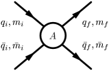
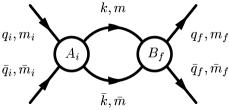
Figure 1: Momenta and masses used in the four point scattering amplitudes and chain links. The center-of-mass momentum is denoted by $p=q_{i}+\bar{q}_{i}=q_{f}+\bar{q}_{f}=k+\bar{k}$.

In this section we introduce our notation for the kinematics of the Bethe-Salpeter equation. We will work in the relativistic framework, restrict ourselves to $s$-waves and put all momenta on-shell (see below). The momenta and masses of a four-point scattering process are given in Fig. 1. A general scalar amplitude $A$ depends only on scalar combinations of the momenta which can be expressed in terms of the Mandelstam variables. The Mandelstam invariants $s$, $t$ and $u$ are defined as the center-of-mass energy squared $s=(q_{i}+\bar{q}_{i})^{2}=p^{2}$, the momentum transfer $t=(q_{i}-q_{f})^{2}$ and the crossed momentum transfer $u=(q_{i}-\bar{q}_{f})^{2}$. The constraint $s+t+u=q_{i}^{2}+\bar{q}_{i}^{2}+q_{f}^{2}+\bar{q}_{f}^{2}=m_{i}^{2}+\bar{m}_{i}^{2}+m_{f}^{2}+\bar{m}_{f}^{2}$ allows one to neglect the combination $t+u$ in favor of $t-u$. The scalar amplitude can be written as $A(s,t-u)$. Since we are only interested in scalar, i.e. $s$-wave or $l=0$, resonances, we must separate channels of different total angular momentum. The amplitude $A$ in our approach is a fourth order polynomial in the momenta. Hence, $A$ can be decomposed as

$$A=\mathop{\textstyle\sum}\nolimits\nolimits_{l}A_{l}J_{l}=A_{s}J_{s}+A_{p}J_{p}+A_{d}J_{d},$$ (1)

where the partial wave operator $J_{l}$ is a polynomial of degree $l$ in $t-u$. The $J_{l}$ read

$$J_{s}= \mathrel{}1,$$

$$J_{p}= \mathrel{}h_{\mu\nu}q_{i}^{\mu}q_{f}^{\nu}=\frac{t-u}{4}+\frac{(q_{i}^{2}-\bar{q}_{i}^{2})(q_{f}^{2}-\bar{q}_{f}^{2})}{4s},$$

$$J_{d}= \mathrel{}D_{\mu\nu\,\rho\sigma}\,q^{\mu}_{i}q^{\nu}_{i}q_{f}^{\rho}q_{f}^{\sigma}=J_{p}^{2}-\frac{h_{\mu\nu}q_{i}^{\mu}q_{i}^{\nu}\,h_{\rho\sigma}q_{f}^{\rho}q_{f}^{\sigma}}{d-1},$$ (2)

and in $d=4$ space-time dimensions they are proportional to Legendre polynomials in the cosine of the scattering angle. The metric $h$ of the $(d-1)$-dimensional space transverse to $p$ is given by

$$h_{\mu\nu}=-g_{\mu\nu}+p_{\mu}p_{\nu}/p^{2}.$$ (3)

The partial wave operators $J_{l}$ can be given in terms of spin projectors, e.g. the spin-$2$ projector

$$D^{\mu\nu}{}_{\rho\sigma}={\textstyle\frac{1}{2}}h^{\mu}_{\rho}h^{\nu}_{\sigma}+{\textstyle\frac{1}{2}}h^{\mu}_{\sigma}h^{\nu}_{\rho}-h^{\mu\nu}h_{\rho\sigma}/(d-1).$$ (4)

The spin projectors are totally symmetric in the upper (lower) indices, orthogonal to $p$ and have the property that every pair of upper (lower) indices is traceless; they project to the spin-$n$ components of a general tensor of rank $n$. This formalism allows us to extract the $s$-wave part of the amplitude $A$.

2.2 Bethe-Salpeter Equation

$$\parbox{85.35826pt}{\centering\includegraphics{scalars2a.eps}\@add@centering}=\parbox{85.35826pt}{\centering\includegraphics{scalars2b.eps}\@add@centering}+\parbox{142.26378pt}{\centering\includegraphics{scalars2c.eps}\@add@centering}$$

Figure 2: Bethe-Salpeter equation for the interaction kernel $A$ (empty circle) and solution $T$ (shaded circle).

The Bethe-Salpeter equation for the two-particle propagator $T$ from a local interaction $A$ is given by [5]

$$T(p,q_{i},q_{f})=A(p,q_{i},q_{f})+\int\frac{i\,d^{d}k}{(2\pi)^{d}}\,\frac{T(p,q_{i},k)A(p,k,q_{f})}{(k^{2}-m^{2})(\bar{k}^{2}-\bar{m}^{2})}.$$ (5)

or diagrammatically in Fig. 2. Combinatorial factors for two identical particles in the loop have to be taken into account, but we prefer to keep this form of the BSE and modify the amplitudes accordingly. In that case $A$ must be the four-point amplitude from ChPT multiplied by $-\frac{1}{2}$ in order for $T$ to be proportional to a bubble chain with the correct factors from perturbation theory. The factor of $\frac{1}{2}$ is the symmetry factor of two identical particle multiplets in a loop and $-1$ stems from factors of $i$ in the vertices and propagators.

We can further simplify the integral in the BSE (5), since we are only interested in the physically relevant piece of the solution $T$ with all momenta put on the mass shell. The amplitude $A$ contains in general off-shell parts which deliver via the integral a contribution even to the on-shell part of the solution $T$. However, these off-shell parts yield exclusively chiral logarithms which – besides being numerically small – can be absorbed by redefining the regularization scale of the loop integral. Furthermore the off-shell parts are not uniquely defined in ChPT. We will therefore set all the momenta in the amplitudes in (5) on-shell. The BSE then simplifies to the arithmetic equation

$$T=A+TGA,$$ (6)

with $G$ being the scalar loop integral in dimensional regularization

$$G_{m\bar{m}}(p^{2})= \mathrel{}\int\frac{i\,d^{d}k}{(2\pi)^{d}}\,\frac{1}{(k^{2}-m^{2})((k-p)^{2}-\bar{m}^{2})}$$

$$= \mathrel{}\frac{1}{16\pi^{2}}\bigg{[}-1+\ln\frac{m\bar{m}}{\mu^{2}}+\frac{m^{2}-\bar{m}^{2}}{p^{2}}\ln\frac{m}{\bar{m}}$$

$$\qquad\qquad\quad\mathord{}-\frac{2\sqrt{\lambda_{m\bar{m}}(p^{2})}}{p^{2}}\mathop{\mathrm{artanh}}\nolimits\frac{\sqrt{\lambda_{m\bar{m}}(p^{2})}}{(m+\bar{m})^{2}-p^{2}}\bigg{]}$$

$$\lambda_{m\bar{m}}(p^{2})= \mathrel{}\big{(}(m-\bar{m})^{2}-p^{2}\big{)}\big{(}(m+\bar{m})^{2}-p^{2}\big{)}.$$ (7)

The scattering matrix $S$ is given by

$$S=1-iCTC\qquad\mbox{with }C^{2}=-2\mathop{\mathrm{Im}}\nolimits G$$ (8)

which is unitary due to the identity $2\mathop{\mathrm{Im}}\nolimits T=-TC^{2}T^{\ast}$. The phase of the unit complex number $S$ is parametrized by the scattering phase $\delta$ defined by $S=\exp(2i\delta)$. For an ideal resonance $\delta$ increases by $180^{\circ}$.

The generalization to $n$ coupled channels is achieved by promoting $A$, $T$, $G$, $C$ and $S$ to $n\times n$ matrices. The matrix $A$ contains the interaction kernels among the channels, $G$ is diagonal with the loop integrals for the channels as elements. The unitary scattering matrix $S$ can be given in terms of eigenvectors and eigenphases.

3 Propagator in the Complex Plane

3.1 Branch cuts

Since the integral has physical significance only for real values of $E=\sqrt{s}$, we will refer to the set of real $E$ as the ‘physical real axis’. In the coupled channel analysis, however, we would like to identify structures on the real axis with poles of the analytic continuation in the lower half of the complex plane. The analytical continuation of $G_{m\bar{m}}(E^{2})$ inherits several branch cuts from its constituent functions and we use the following conventions. The branch cut of $\sqrt{x}$ is just below the negative real axis, the branch cuts of $\mathop{\mathrm{artanh}}\nolimits{x}$ are below the negative real axis from $-1$ and above the real axis from $+1$. The resulting branch cut in $I$ is below the positive real axis of $E$ starting at the threshold point $m+\bar{m}$. This Riemann sheet is commonly referred to as the ‘physical’ sheet.

Figure 3: Branch cuts in ‘physical’ sheet (left) and our choice of Riemann sheet (right). Shown are paths from points $E_{i}$ to the physical real axis $E\in{\mathbb{R}}$. The branching point $m+\bar{m}$ is moved slightly down for reasons of presentation.

Unfortunately, it is not well suited for finding physically relevant poles. This can be seen as follows: a relevant pole is a pole in the lower half of the complex plane and close to the physical real axis which has a strong influence on observables. Points $E$ in the upper half of the complex plane or below threshold (e.g. $E_{1}$, $E_{2}$, $E_{3}$ in Fig. 3 left) can be connected with a straight vertical line $\gamma$ ($\gamma_{1}$, $\gamma_{2}$, $\gamma_{3}$) to the physical real axis. The length of $\gamma$ is $|\mathop{\mathrm{Im}}\nolimits p|$ and $E$ is as close to the physical real axis as possible. Points $E$ in the lower half of the complex plane above threshold (e.g. $E^{\prime}_{4}$), on the other hand, are not close to the physical real axis, because the length of the paths connecting $E$ to the physical real axis (such as $\gamma^{\prime}_{4}$, $\gamma^{\prime\prime}_{4}$) exceeds $|\mathop{\mathrm{Im}}\nolimits E|$. The vertical path towards the real axis ($\gamma^{\prime\prime\prime}_{4}$) crosses the branch cut and ends in an unphysical real axis.

As a matter of fact, the region below the physical real axis and above threshold turns out to be the most interesting of all, because here physically relevant poles occur. Therefore it is better to consider the ‘physical’ sheet with the branch cut rotated down by $90^{\circ}$ (Fig. 3 right). Every point in that rotated sheet is as close as possible to the physical real axis and the loop integral function defined on the rotated sheet is

$$G_{m\bar{m}}(E^{2})\mapsto G_{m\bar{m}}(E^{2})-\frac{\sqrt{-\lambda_{m\bar{m}}(E^{2})}}{8\pi E^{2}}\,\theta\bigl{(}-\mathop{\mathrm{Im}}\nolimits E\bigr{)}\,\theta\bigl{(}\mathop{\mathrm{Re}}\nolimits(E-m-\bar{m})\bigr{)},$$ (9)

with $\theta(x)$ being the unit step function with $\theta(0)=0$. With this choice for the analytic continuation of the loop integral most poles that are relevant for the physical real axis – except those which are related to cusps (cf. next section) – are in the same sheet, whereas other investigations have to take several sheets into account, in order to observe the physically relevant poles.

Figure 4: A cusp at threshold and the corresponding pair of poles. The branch cut can be perturbed so that both poles reside on the same Riemann sheet.

3.2 Cusps

When the modified integral (9) is used for all channels in a coupled channel approach, most of the poles can be seen simultaneously. Nevertheless, some relevant poles may still be hidden behind a branch cut. This is the case if there are cusp resonances in the spectrum. Cusps are discontinuities of the derivative of the full amplitude and they occur at the threshold energy of each channel. Cusp resonances can be generated by the configuration of poles as shown in Fig. 4. In the rotated Riemann sheet no poles are seen, but there is one pole just behind the branch cut on either side. When the branch cut is moved around these two poles the situation becomes clearer. The real axis below threshold is close to the pole at $E_{1}$. The amplitude will therefore have a peak at $\mathop{\mathrm{Re}}\nolimits E_{1}$, but only the increase on the right of the resonance is below threshold and physical; the peak itself lies on an unphysical real axis. Above threshold it is just the opposite, the peak at $\mathop{\mathrm{Re}}\nolimits E_{2}$ is hidden and only the decline on the left is physical. The cusp resonance is therefore the interplay between two poles and a branch cut. It is even more instructive to consider both poles as manifestations of the same pole disturbed by the branch cut singularity: At a pole the denominator is zero. Going from one sheet to another corresponds to adding some function to the propagator integral in the denominator. Assuming this function to be small, the root will be shifted by a small amount giving rise to a nearby pole on the new sheet. When $E_{1}$ and $E_{2}$ are considered one, the cusp can be considered as a common resonance with the middle part removed by the branch cut. In the scattering phase a cusp will correspond to an increase of considerably less than $\pi$ as for usual resonances, because the sharp increase at the center is eliminated.

4 Results and Comparison

We can now employ the Bethe-Salpeter equation as presented in Sec. 2, in order to fit to scattering data of two pseudoscalar mesons. In $U(3)$ ChPT the fundamental pseudoscalar mesons are the Goldstone bosons $(\pi,K,\eta)$ with their singlet counterpart, the $\eta^{\prime}(958)$. The potential $A$ is derived from the chiral $U(3)$ Lagrangian by calculating the tree diagrams up to fourth chiral order and taking $\eta$-$\eta^{\prime}$ mixing into account where we employ the two-mixing angle scheme as described in [9]. Tadpoles and crossed diagrams which are not included in our approach have been shown to yield numerically small effects in scattering processes in the physical region and can furthermore be partially absorbed by redefining chiral parameters. We have therefore neglected both tadpoles and crossed diagrams and restrict ourselves to the tree diagrams in the calculation of the potential $A$.

We work with the Lagrangian found in [9, 19]

$${\mathcal{L}}= \mathrel{}{\textstyle\frac{1}{4}}f^{2}\langle\partial^{\mu}U^{\dagger}\partial_{\mu}U\rangle+{\textstyle\frac{1}{2}}f^{2}\mathop{\mathrm{Re}}\nolimits\langle U^{\dagger}\chi\rangle+i{\textstyle\frac{1}{3}}\sqrt{6}\,v_{3}^{(1)}(\ln\det U)\mathop{\mathrm{Im}}\nolimits\langle U^{\dagger}\chi\rangle+{\textstyle\frac{1}{12}}f^{2}m_{0}^{2}(\ln\det U)^{2}$$ (10)

$$\mathord{}+\beta_{0}^{(0)}\langle\partial^{\mu}U^{\dagger}\partial^{\nu}U\partial_{\mu}U^{\dagger}\partial_{\nu}U\rangle+\beta_{3}^{(0)}\langle\partial^{\mu}U^{\dagger}\partial_{\mu}U\partial^{\nu}U^{\dagger}\partial_{\nu}U\rangle$$

$$\mathord{}+2\beta_{5}^{(0)}\mathop{\mathrm{Re}}\nolimits\langle\partial^{\mu}U^{\dagger}\partial_{\mu}UU^{\dagger}\chi\rangle+2\beta_{8}^{(0)}\mathop{\mathrm{Re}}\nolimits\langle U^{\dagger}\chi U^{\dagger}\chi\rangle+\ldots$$

where $\chi=2B\mathop{\mathrm{diag}}\nolimits(\hat{m},\hat{m},m_{s})$ is the quark mass matrix in the isospin limit and $m_{0}$ denotes the mass of the $\eta^{\prime}$ in the chiral limit. We have omitted all terms that are irrelevant or are not considered here, in particular we have only taken the most relevant terms from the fourth chiral order Lagrangian according to the OZI rule. We replace the quark masses $\hat{m}$, $m_{s}$ and the constant $f$ by the fourth chiral order expressions (without loops) for the pion, kaon masses $M_{\pi}=138\,\mathrm{MeV}$, $M_{K}=496\,\mathrm{MeV}$ and the pion decay constant $F_{\pi}=92.4\,\mathrm{MeV}$. The interaction kernel $A$ for the Bethe-Salpeter equation are the tree level amplitudes from the Lagrangian separated in angular momentum and isospin channels. As an example we state the $4\pi$ vertex with $J=0$, $I=2$,

$$A=\frac{s-2M_{\pi}^{2}}{2F_{\pi}^{2}}-\frac{4\beta_{0}^{(0)}}{F_{\pi}^{4}}\bigl{(}s-2M_{\pi}^{2}\bigr{)}^{2}-\frac{4\beta_{3}^{(0)}}{3F_{\pi}^{4}}\bigl{(}4M_{\pi}^{4}-2M_{\pi}^{2}s+s^{2}\bigr{)}+\frac{4\beta_{5}^{(0)}M_{\pi}^{2}s}{F_{\pi}^{4}}-\frac{16\beta_{8}^{(0)}M_{\pi}^{4}}{F_{\pi}^{4}}.$$

For the particle propagators we use the standard propagators for scalar particles with the physical masses of the particles.

In this section we present a fit to scattering data from [20] ($K\pi$), [21, 22] ($\pi\pi$, $I=2$) and [23]. The work [23] is a collection of $\pi\pi$ scattering data from [21, 22, 24, 25, 26, 27, 28, 29, 30, 31, 32, 33, 34, 35, 36, 37, 38] and $K\pi$ scattering data from [39, 40]. Having replaced the quark masses and $f$ by the meson masses and $F_{\pi}$ as described above, the only free parameters left are the regularization scale $\mu$ in $G$ and the coupling constants of the effective Lagrangian.

4.1 SU(3) ChPT

We first restrict ourselves to the conventional chiral $SU(3)$ Lagrangian. This is done by omitting all possible vertices which include the $\eta^{\prime}$ field. Later on we will proceed by including the $\eta^{\prime}$ field explicitly. By comparison we can then pin down the effects of the $\eta^{\prime}$ within this approach. The parameters entering in the pure $SU(3)$ case are besides the regularization scale $\mu$ only the known parameters $\beta_{k}$, $k=0,\ldots,8$, from $SU(3)$ ChPT. However, there is a slight difference in so far as that we keep the low-energy constant (LEC) $\beta_{0}$ from the fourth order Lagrangian explicitly. Usually this contact term is absorbed into other terms of the Lagrangian by employing a Cayley-Hamilton matrix identity [19], but for processes including the $\eta^{\prime}$ it seems to be more convenient to keep this term [41]. The values of some of the LECs $\beta_{k}$, involved in the Cayley-Hamilton identity change accordingly. The LECs $\beta_{1}$, $\beta_{2}$, $\beta_{4}$, $\beta_{6}$, and $\beta_{7}$ are then compatible with zero within their phenomenologically determined error bars and we neglect them as an approximation. This estimate for the LECs has been proven to be quite successful in [9, 41] and suggests that the important physics for the considered processes is included in the remaining parameters $\beta_{0}$, $\beta_{3}$, $\beta_{5}$, and $\beta_{8}$. The omission of the first parameters is also motivated by the observation that they can be interpreted as OZI violating corrections of the latter ones. Of course, an improved fit to data might be obtained by fine-tuning these suppressed parameters, but no additional insight is gained and none of our conclusions change. We therefore consider the reduced set of parameters $\beta_{0}^{(0)},\beta_{3}^{(0)},\beta_{5}^{(0)}$ and $\beta_{8}^{(0)}$ with their values given by

$$\begin{array}[]{lll}\beta_{0}^{(0)}=(0.6\pm 0.1)\times 10^{-3},&&\beta_{3}^{(0)}=(-0.5\pm 0.1)\times 10^{-3},\\ \beta_{5}^{(0)}=(1.4\pm 0.2)\times 10^{-3},&&\beta_{8}^{(0)}=(0.2\pm 0.2)\times 10^{-3}.\end{array}$$ (11)

while neglecting the remaining LECs $\beta_{k}$. Using this set of parameters we will compare the results for the phase shifts with available experimental data. The results presented in the paper have been obtained by employing the central values for the LECs in Eq. (11), but variations within the given ranges for the parameters do not lead to substantial differences in the results. We furthermore restricted ourselves first to a single scale parameter $\mu=1\,\mathrm{GeV}$ for all channels and energies. However, with such a simplified choice the calculated phase in the $I={\textstyle\frac{1}{2}}$ channel turned out to be slightly above the data points. This feature can also be seen in [4, 42]. By lowering the scale down to $\mu=0.8\,\mathrm{GeV}$ in that particular channel we are easily able to improve the fit. This indicates that our approach neglects further contributions in the $I={\textstyle\frac{1}{2}}$ channel which we mimic by fine-tuning the scale $\mu$. The results are summarized in Tab. 1 and Fig. 5.

$$\begin{array}[]{|ll|c|}\hline\cr I&\mbox{resonance}&\mbox{pole}\\ \hline\cr 0&f_{0}(400-1200)&\phantom{0}448-263i\\ 0&f_{0}(980)&\phantom{0}983-\phantom{0}14i\\ {\textstyle\frac{1}{2}}&K_{0}^{*}(900)&\phantom{0}740-246i\\ 1&a_{0}(980)^{<}&1081-\phantom{0}36i\\ 1&a_{0}(980)^{>}&\phantom{0}791-\phantom{0}75i\\ \hline\cr\end{array}$$

Table 1: Pole positions (MeV) of scalar channels from the $SU(3)$ chiral Lagrangian and using the parameter set in (11).

In the $I=0$ channel matching is remarkable up to energies around $E_{\mathrm{cm}}=1.2\,\mathrm{GeV}$, the linear increase from threshold to just below $1\,\mathrm{GeV}$ is due to the $\sigma$ or $f_{0}(400-1200)$ resonance and the $f_{0}(980)$ resonance can be clearly seen by a sudden phase shift of $180^{\circ}$. These resonances are associated with poles at $(448-263i)\,\mathrm{MeV}$ and $(983-14i)\,\mathrm{MeV}$. This is in reasonable agreement with recent results for light scalar mesons obtained from Dalitz plot analyses of charm decays in the Fermilab experiment E791 [43]. By analyzing the decay $D^{+}\rightarrow\pi^{-}\pi^{+}\pi^{+}$ [44] strong evidence of the $\sigma$ was found with a mass of $478\pm 17\,\mathrm{MeV}$ and a width of $324\pm 21\,\mathrm{MeV}$ which corresponds to twice the imaginary part of the pole position. From the analysis of the $D_{s}^{+}\rightarrow\pi^{-}\pi^{+}\pi^{+}$ decay [45] the mass and the width of the $f_{0}(980)$ were remeasured to be $975\pm 3\,\mathrm{MeV}$ and $44\pm 4\,\mathrm{MeV}$, respectively.

Our results start deviating from the experimental phase shifts at around $E_{\mathrm{cm}}=1.2\,\mathrm{GeV}$, however, this is not very surprising since higher particle effects which are omitted in this scheme, in particular the $4\pi$ channel, will become important at these energies [46]. In the $I={\textstyle\frac{1}{2}}$ channel a broad resonance, the $\kappa$ or $K_{0}^{\ast}(900)$, can be seen extending from threshold to about $1\,\mathrm{GeV}$, which is related to a pole at $(740-246i)\,\mathrm{MeV}$. Again, we have good agreement with data up to energies of $E_{\mathrm{cm}}=1.3\,\mathrm{GeV}$. In the $I=1$ channel a sharp increase just below $1\,\mathrm{GeV}$ is due to the $a_{0}(980)$ resonance, which manifests as a cusp in the scattering amplitude. A possible cusp interpretation of the $a_{0}$ has already been given in [47]. In our analysis it corresponds to poles at $(1081-36i)\,\mathrm{MeV}$ and $(791-75i)\,\mathrm{MeV}$ (see the discussion about cusps in Sec. 3). These poles are both hidden on our standard Riemann sheet, the first pole lies on the Riemann sheet corresponding to the physical region between the branching points of $\pi\eta$ at $682\,\mathrm{MeV}$ and $KK$ at $988\,\mathrm{MeV}$ and the second one corresponding to the Riemann sheet above the $KK$ branching point. Therefore, the $a_{0}$ appears as a resonance with its central part cut away and the phase shift is less than $180^{\circ}$. For the $I={\textstyle\frac{3}{2}}$ and $I=2$ channels reasonable agreement with experiment is achieved for center-of mass energies up to $E_{\mathrm{cm}}=1.5\,\mathrm{GeV}$ and no significant increase of the phase shifts is observed.

4.2 U(3) ChPT

We now extend the chiral Lagrangian to its $U(3)$ form by including the $\eta^{\prime}$ explicitly. In order to compare the results with the pure $SU(3)$ analysis we make the same choice for the parameters (11), while the additional LECs of the $U(3)$ Lagrangian are set to zero. This approximation yields good results and we refrain from performing a better fit to existing data by fine-tuning the new couplings. The resulting scattering phases are shown in Fig. 6 and the pole positions are given in Tab. 2. We note that up to $1.5\,\mathrm{GeV}$ there are no considerable differences to $SU(3)$ ChPT. In particular, the inclusion of the $\eta^{\prime}$ channels does not yield any new resonances in the considered energy range up to $1.5\,\mathrm{GeV}$.

$$\begin{array}[]{|ll|c|}\hline\cr I&\mbox{resonance}&\mbox{pole}\\ \hline\cr 0&f_{0}(400-1200)&\phantom{0}459-233i\\ 0&f_{0}(980)&\phantom{0}994-\phantom{0}10i\\ {\textstyle\frac{1}{2}}&K_{0}^{*}(900)&\phantom{0}737-248i\\ 1&a_{0}(980)^{<}&1061-\phantom{0}55i\\ 1&a_{0}(980)^{>}&\phantom{0}761-\phantom{0}62i\\ \hline\cr\end{array}$$

Table 2: Pole positions (MeV) of scalar channels from the $U(3)$ chiral Lagrangian and using the parameter set in (11).

This is a non-trivial observation, since the inclusion of $\eta^{\prime}$ channels might have disturbed the agreement with experimental data of the pure $SU(3)$ case via coupling between the channels as has been observed in the meson-baryon sector [7]. In the purely mesonic sector, on the other hand, the effects of the $\eta^{\prime}$ decouple to a large extent from the interactions of the Goldstone bosons. Remarkably, the results are insensitive to the value of $\tilde{v}_{2}^{(1)}={\textstyle\frac{1}{4}}f^{2}-{\textstyle\frac{1}{2}}\sqrt{6}v_{3}^{(1)}$ which is mainly responsible for $\eta\eta^{\prime}$ mixing [9]. Variation of its value from $\tilde{v}_{2}^{(1)}={\textstyle\frac{1}{4}}f^{2}$ with omitted $1/N_{c}$-suppressed piece $v_{3}^{(1)}$ down to $\tilde{v}_{2}^{(1)}=0$ for suppressed mixing does not alter our results considerably.

The similarity of the $SU(3)$ and $U(3)$ results with the same set of parameters depends on a Cayley-Hamilton identity which can be utilized to absorb the parameter $\beta_{0}$ by some of the other LECs. In the $SU(3)$ case this identitiy involves the parameters $\beta_{0},\ldots,\beta_{3}$, whereas for $U(3)$ the additional parameters $\beta_{13},\ldots,\beta_{16}$ are included, see [41]. Our choice of setting the new parameters $\beta_{13},\ldots,\beta_{16}$ to zero does not change the results with respect to the $SU(3)$ case, since we kept $\beta_{0}$ explicitly. If, on the other hand, we would have preferred to absorb $\beta_{0}$, the equivalence of both schemes could have only been restored by taking non-vanishing values for $\beta_{13},\ldots,\beta_{16}$ in the $U(3)$ Lagrangian as given by the Cayley-Hamilton identity.

There are, however, small differences between the $SU(3)$ and $U(3)$ results, if the same set of parameters is employed, and they are most easily seen in the positions of the poles in Tab. 1 and Tab. 2 which change by up to $30\,\mathrm{MeV}$. These changes give a measure for the importance of the $\eta^{\prime}$ contributions within this approach. In the $SU(3)$ framework some effects of the $\eta^{\prime}$ are hidden in the coupling constants of the fourth order chiral Lagrangian [9, 11, 12], whereas in the $U(3)$ theory the $\eta^{\prime}$ is treated as a dynamical degree of freedom. Hence, in order to reproduce the $SU(3)$ results more accurately, the coupling constants would have to be modified slightly compensating the $\eta^{\prime}$ contributions in the $U(3)$ framework.

4.3 Comparison with previous work

It is instructive to compare the present investigation with previous work on coupled meson channels. In [3] the second order $SU(3)$ Lagrangian was sufficient to reproduce the measured scattering data below $1\,\mathrm{GeV}$. This work was done in cut-off regularization and with a reduced set of channels. When setting all fourth order couplings to zero in our approach we obtain very similar scattering data, with or without the $\eta^{\prime}$ channels, which shows that at leading order the $\eta^{\prime}$ has hardly any effect on low energy physics.

In [4], for example, the approach was extended by including the fourth order Lagrangian and a full analysis of the scalar and vector channels in $SU(3)$ ChPT was performed. By adjusting the LECs the authors were able to obtain good agreement for all presented data. The main difference to our scheme is the expansion of the scattering amplitude. For the amplitude $A$ at a vertex we use the sum of the second and fourth order amplitudes $A=A_{2}+A_{4}$, whereas in [4] the inverse amplitude (IAM) expansion

$$A=A_{2}(A_{2}-A_{4})^{-1}A_{2}=A_{2}+A_{4}+A_{4}A_{2}^{-1}A_{4}+\ldots$$ (12)

was used which is equal in fourth order. Both approaches differ significantly at energies well above $E_{\mathrm{cm}}=1\,\mathrm{GeV}$. This difference can be easily understood by investigating the asymptotic dependence of $A$ with respect to the energy squared $s$. The amplitudes $A_{2}$ and $A_{4}$ are linear and quadratic in $s$, respectively. While in our scheme the introduction of fourth order couplings increases the asymptotic power of $A$ to two, it is decreased to zero in the other scheme.

In a couple of papers on this subject the results were refined. In the work [48] a full IAM analysis with manifest regularization independence, but without manifest unitarity is performed. The main advantage of this approach is the direct compatibility with chiral perturbation theory from which the one-loop amplitude is taken. Here, the $K\pi$, $I={\textstyle\frac{1}{2}}$, scattering phase agrees with the experimental data. This is possibly due to the $t$ and $u$ channel loops that are included in the full IAM analysis. When they are dropped as in [4] or our analysis the scattering phase is increased. The effect of those loops can be simulated by a change of renormalization scale, this is what we did by lowering $\mu$ to $0.8\,\mathrm{GeV}$ in this particular channel.

Finally, we would like to comment on a possible extension to $SU(3)$ or $U(3)$ of the $SU(2)$ analysis described in [5] where emphasis was put on renormalization. For each channel a separate counterterm polynomial was introduced to account for the infinities of the loop integral. The success of this method relies on the fact that there are only three channels in $SU(2)$, $\pi\pi$ with $(I,J)$ equals $(0,0)$, $(1,1)$ and $(2,0)$. In $SU(3)$ or $U(3)$ ChPT, however, more than ten channels exist and each of them would require different coefficients for the polynomials. With such a large number of coefficients agreement with experimental data is easily achieved without constraining most of the parameters and the method would lose its predictive power.

5 Conclusions

In this work we have analyzed meson-meson scattering from the $SU(3)$ and $U(3)$ chiral effective Lagrangians in the $s$-wave channel by means of a coupled channel Bethe-Salpeter equation. We have presented the Bethe-Salpeter equation and solved it for a local interaction kernel. Resonances are identified by relating them to poles in the analytical continuation of the scattering cross section and multiplets of composed states of two fundamental pseudoscalar mesons, i.e. $(\pi,K,\eta,\eta^{\prime})$, are discussed.

We first investigated the $SU(3)$ case. The fourth order Lagrangian was simplified by taking only the most relevant parameters according to the OZI rule into account, which are $\beta_{0}^{(0)}$, $\beta_{3}^{(0)}$, $\beta_{5}^{(0)}$ and $\beta_{8}^{(0)}$. In the isospin $I=0$ and $I={\textstyle\frac{1}{2}}$ channels we were able to fit the scattering phases up to about $1.2$-$1.3\,\mathrm{GeV}$, in analogy to results found, e.g., in [4]. Above $1.2\,\mathrm{GeV}$ deviations from the experimental phase shifts are observed as expected due to the omission of higher particle states, e.g., the $4\pi$ channel should become important in the $I=0$ channel at these energies. For the $I={\textstyle\frac{3}{2}}$ and $I=2$ channels reasonable agreement with experiment is achieved for center-of mass energies up to $1.5\,\mathrm{GeV}$ and no significant increase of the phase shifts is observed.

In a second step, the analysis was extended to $U(3)$ ChPT by including the $\eta^{\prime}$ explicitly. Employing the same choice for the LECs as in the $SU(3)$ case and neglecting new couplings of the $\eta^{\prime}$ which are also OZI suppressed (more generally: the 1/$N_{c}$ suppressed couplings) the results in this energy region were not altered considerably and again the spectrum could be reproduced. This is a non-trivial statement, since the coupling between the $\eta^{\prime}$ channels with the other ones may have destroyed the agreement of the pure $SU(3)$ case, and is in contradistinction to the results recently obtained in the meson-baryon sector [7]. Nevertheless, small effects from the inclusion of the $\eta^{\prime}$ are observed which would require a slight readjustment of the coupling constants, in order to reproduce the results of the $SU(3)$ case. In our approach and with our choice of the parameter values the inclusion of the $\eta^{\prime}$ does not yield new resonances below $1.5\,\mathrm{GeV}$ that could be interpreted as quasi-bound states of the $\eta^{\prime}$ with a Goldstone boson.

We should mention that our fit to the phase shifts is not unique. The OZI violating parameters which we have neglected here do not necessarily need to be small and can contribute to meson-meson scattering. However, a small variation of these parameters could always be compensated by small variations of $\beta_{0}^{(0)}$, $\beta_{3}^{(0)}$, $\beta_{5}^{(0)}$ and $\beta_{8}^{(0)}$. The choice of the parameters made in the present investigation is in so far appealing as it takes only a minimal set of four LECs into account while setting the remaining OZI violated couplings to zero. Further phenomenological input such as the three pion decays of the $\eta$ and $\eta^{\prime}$ [49] may help to extract the values of some of the LECs more precisely and clarify if this simplifying assumption for the LECs was justified.

Figures

Figure 5: Scattering data from $SU(3)$ chiral Lagrangians and experimental data from [23] (all plots), [20] ($K\pi$), [21, 22] ($\pi\pi$, $I=2$). The $S$-matrix elements are parametrized as $S=\sqrt{2\zeta}e^{2i\delta}$ where $\delta$ is the phase and $\zeta$ the magnitude.

Figure 6: Scattering data from $U(3)$ chiral Lagrangians with experimental data points from [23] (all plots), [20] ($K\pi$), [21, 22] ($\pi\pi$, $I=2$). The $S$-matrix elements are parametrized as $S=\sqrt{2\zeta}e^{2i\delta}$ where $\delta$ is the phase and $\zeta$ the magnitude.

References

- [1] N. Kaiser, P. B. Siegel and W. Weise, “Chiral dynamics and the low-energy interaction”, Nucl. Phys. A594 (1995) 325, nucl-th/9505043.
- [2] N. Kaiser, T. Waas and W. Weise, “ chiral dynamics with coupled channels: and photoproduction”, Nucl. Phys. A612 (1997) 297, hep-ph/9607459.
- [3] J. A. Oller and E. Oset, “Chiral symmetry amplitudes in the s-wave isoscalar and isovector channels and the , , scalar mesons”, Nucl. Phys. A620 (1997) 438, hep-ph/9702314.
- [4] J. A. Oller, E. Oset and J. R. Pelaez, “Meson meson and meson baryon interactions in a chiral non-perturbative approach”, Phys. Rev. D59 (1999) 074001, hep-ph/9804209.
- [5] J. Nieves and E. Ruiz Arriola, “Bethe-Salpeter approach for unitarized chiral perturbation theory”, Nucl. Phys. A679 (2000) 57, hep-ph/9907469.
- [6] J. Caro Ramon, N. Kaiser, S. Wetzel and W. Weise, “Chiral dynamics with coupled channels: Inclusion of p-wave multipoles”, Nucl. Phys. A672 (2000) 249, nucl-th/9912053.
- [7] S. D. Bass, S. Wetzel and W. Weise, “Axial dynamics in and photoproduction”, Nucl. Phys. A686 (2001) 429, hep-ph/0007293.
- [8] R. Kaiser and H. Leutwyler, “Large in chiral perturbation theory”, Eur. Phys. J. C17 (2000) 623, hep-ph/0007101.
- [9] N. Beisert and B. Borasoy, “ mixing in chiral perturbation theory”, Eur. Phys. J. A11 (2001) 329, hep-ph/0107175.
- [10] S. Wetzel, private communication.
- [11] G. Ecker, J. Gasser, A. Pich and E. de Rafael, “The role of resonances in chiral perturbation theory”, Nucl. Phys. B321 (1989) 311.
- [12] P. Herrera-Siklody, “Matching of and chiral perturbation theories”, Phys. Lett. B442 (1998) 359, hep-ph/9808218.
- [13] A. Abele, “ annihilation at rest into ”, Phys. Rev. D57 (1998) 3860.
- [14] Crystal Barrel Collaboration, C. Amsler et al., “High statistics study of decay into ”, Phys. Lett. B353 (1995) 571.
- [15] S. D. Bass and E. Marco, “Final state interaction and a light mass ’exotic’ resonance”, Phys. Rev. D65 (2002) 057503, hep-ph/0108189.
- [16] E852 Collaboration, D. R. Thompson et al., “Evidence for exotic meson production in the reaction at ”, Phys. Rev. Lett. 79 (1997) 1630, hep-ex/9705011.
- [17] E852 Collaboration, E. I. Ivanov et al., “Observation of exotic meson production in the reaction at ”, Phys. Rev. Lett. 86 (2001) 3977, hep-ex/0101058.
- [18] Crystal Barrel Collaboration, A. Abele et al., “Exotic state in anti- annihilation at rest into (spectator)”, Phys. Lett. B423 (1998) 175.
- [19] P. Herrera-Siklody, J. I. Latorre, P. Pascual and J. Taron, “Chiral effective Lagrangian in the large- limit: The nonet case”, Nucl. Phys. B497 (1997) 345, hep-ph/9610549.
- [20] R. Mercer et al., “ scattering phase shifts determined from the reactions and ”, Nucl. Phys. B32 (1971) 381.
- [21] W. Hoogland et al., “Isospin-two phase shifts from an experiment at ”, Nucl. Phys. B69 (1974) 266.
- [22] M. J. Losty et al., “A study of -scattering from interactions at ”, Nucl. Phys. B69 (1974) 185.
- [23] T. Ishida, “- scattering phaseshift database”, http://amaterasu.kek.jp/sigma/database/pipip/.
- [24] J. P. Baton, G. Laurens and J. Reignier, “ phase shifts from Chew-Low extrapolations of at ”, Phys. Lett. B33 (1970) 528.
- [25] J. P. Baton, G. Laurens and J. Reignier, “ elastic cross section from Chew-Low extrapolations of reaction at ”, Phys. Lett. B33 (1970) 525.
- [26] N. M. Cason et al., “Study of scattering amplitudes in the reaction at ”, Phys. Rev. D28 (1983) 1586.
- [27] P. Estabrooks and A. D. Martin, “ phase shift analysis below the threshold”, Nucl. Phys. B79 (1974) 301.
- [28] S. D. Protopopescu et al., “ partial wave analysis from reactions and at ”, Phys. Rev. D7 (1973) 1279.
- [29] L. Rosselet et al., “Experimental study of K(e) decays”, Phys. Rev. D15 (1977) 574.
- [30] V. Srinivasan et al., “ interactions below from data at ”, Phys. Rev. D12 (1975) 681.
- [31] D. H. Cohen, T. Ferbel, P. Slattery and B. Werner, “Study of scattering in the isotopic spin- channel”, Phys. Rev. D7 (1973) 661.
- [32] E. Colton et al., “Measurement of elastic cross sections”, Phys. Rev. D3 (1971) 2028.
- [33] J. P. Prukop et al., “ scattering below from at ”, Phys. Rev. D10 (1974) 2055.
- [34] W. Hoogland et al., “Measurement and analysis of the system produced at small momentum transfer in the reaction at ”, Nucl. Phys. B126 (1977) 109.
- [35] J. H. Scharenguivel, L. J. Gutay, D. H. Miller, F. T. Meiere and S. Marateck, “Experimental determination of the low mass I=0 s-wave phase shift using a method which is consistent with the off-mass-shell dependence of current algebra”, Nucl. Phys. B22 (1970) 16.
- [36] B. Hyams et al., “ phase shift analysis from to ”, Nucl. Phys. B64 (1973) 134.
- [37] A. Zylbersztejn et al., “Further results on K(e) decay and energy dependence of low-energy phase shift”, Phys. Lett. B38 (1972) 457.
- [38] G. Grayer et al., “High statistics study of the reaction : Apparatus, method of analysis, and general features of results at ”, Nucl. Phys. B75 (1974) 189.
- [39] D. Aston et al., “A study of scattering in the reaction at ”, Nucl. Phys. B296 (1988) 493.
- [40] P. Estabrooks et al., “Study of scattering using the reactions and at ”, Nucl. Phys. B133 (1978) 490.
- [41] N. Beisert and B. Borasoy, “The decay in chiral perturbation theory”, Nucl. Phys. A705 (2002) 433, hep-ph/0201289.
- [42] J. A. Oller, E. Oset and J. R. Pelaez, “The decay within a chiral unitary approach”, Phys. Rev. D62 (2000) 114017, hep-ph/9911297.
- [43] Fermilab E791 Collaboration, I. Bediaga, “Light scalar mesons and in charm meson decays”, hep-ex/0208039.
- [44] E791 Collaboration, E. M. Aitala et al., “Experimental evidence for a light and broad scalar resonance in decay”, Phys. Rev. Lett. 86 (2001) 770, hep-ex/0007028.
- [45] E791 Collaboration, E. M. Aitala et al., “Study of the decay and measurement of masses and widths”, Phys. Rev. Lett. 86 (2001) 765, hep-ex/0007027.
- [46] R. Kaminski, L. Lesniak and B. Loiseau, “Three channel model of meson meson scattering and scalar meson spectroscopy”, Phys. Lett. B413 (1997) 130, hep-ph/9707377.
- [47] M. Uehara, “Revisit to low mass scalar mesons via unitarized chiral perturbation theory”, hep-ph/0204020.
- [48] A. Gomez Nicola and J. R. Pelaez, “Meson meson scattering within one loop chiral perturbation theory and its unitarization”, Phys. Rev. D65 (2002) 054009, hep-ph/0109056.
- [49] N. Beisert and B. Borasoy, “Hadronic decays of and with coupled channels”, hep-ph/0301058, to appear in Nucl. Phys. A.