hep-ph/0302021

IFIC/03-03

ZU-TH02/03

Solar Neutrino Masses and Mixing from Bilinear R-Parity Broken Supersymmetry: Analytical versus Numerical Results

M. A. Díaz1, M. Hirsch2, W. Porod3, J. C. Romão2,4 and J. W. F. Valle2

1 Facultad de Física, Universidad Católica de Chile
Av. Vicuña Mackenna 4860, Santiago, Chile

2 AHEP Group, Instituto de Física Corpuscular – C.S.I.C./Universitat de València
Edificio de Institutos de Paterna, Apartado 22085, E–46071 València, Spain

3 Institut für Theoretische Physik, Universität Zürich,
CH-8057 Zürich, Switzerland

4 Departamento de Física and CFIF, Instituto Superior Técnico
Av. Rovisco Pais 1,    1049-001 Lisboa, Portugal

We give an analytical calculation of solar neutrino masses and mixing at one-loop order within bilinear R-parity breaking supersymmetry, and compare our results to the exact numerical calculation. Our method is based on a systematic perturbative expansion of R-parity violating vertices to leading order. We find in general quite good agreement between approximate and full numerical calculation, but the approximate expressions are much simpler to implement. Our formalism works especially well for the case of the large mixing angle MSW solution (LMA-MSW), now strongly favoured by the recent KamLAND reactor neutrino data.

1 Introduction

Solar neutrino experiments, including the measurement of the neutral current rate for solar neutrinos by the SNO collaboration Ahmad:2002jz provide a solid evidence for solar neutrino conversions Maltoni:2002ni . This has been recently confirmed by the first results from the KamLAND experiment using reactor (anti)-neutrinos :2002dm , Pakvasa:2003zv . Combining the information from reactors with all of the solar neutrino data leads to the best fit point Maltoni:2002aw :

tan2θsol=0.46,Δm2sol=6.9×10⁵eV2,formulae-sequencesuperscript2𝜃𝑠𝑜𝑙0.46Δsuperscript𝑚2𝑠𝑜𝑙6.9superscript105superscripteV2\tan^{2}\theta{sol}=0.46,\qquad\Delta m^{2}{sol}=6.9\times 10^{-5}~{}\rm{eV}^{2}\,, (1)

confirming that the solar neutrino mixing angle is large, but significantly non-maximal. The 3σ3𝜎3\sigma region for θ𝜃\theta is:

0.29tan2θsol0.86,0.29superscript2𝜃𝑠𝑜𝑙0.860.29\leq\tan^{2}\theta{sol}\leq 0.86, (2)

based on a combination of all experimental data. However, one finds a significant reduction of the allowed Δm2solΔsuperscript𝑚2𝑠𝑜𝑙\Delta m^{2}{sol} range. As shown in Ref. Maltoni:2002aw , the pre-KamLAND LMA-MSW region is now split into two sub-regions. At 3σ3𝜎3\sigma (1 dof.) one obtains

5.1×10⁵eV2Δm2sol9.7×105eV2,1.2×104eV2Δm2sol1.9×104eV2.formulae-sequence5.1superscript105superscripteV2Δsuperscriptm2sol9.7superscript105superscripteV21.2superscript104superscripteV2Δsuperscriptm2sol1.9superscript104superscripteV25.1\times 10^{-5}~{}\rm{eV}^{2}\leq\Delta m^{2}{sol}\leq 9.7\times 10^{-5}~{}\rm{eV}^{2},\\ 1.2\times 10^{-4}~{}\rm{eV}^{2}\leq\Delta m^{2}{sol}\leq 1.9\times 10^{-4}~{}\rm{eV}^{2}. (3)

Altogether, KamLAND results exclude all oscillation solutions except for the large mixing angle MSW solution (LMA-MSW) to the solar neutrino problem Gonzalez-Garcia:1999aj .

On the other hand, current atmospheric neutrino data require oscillations involving νμντsubscript𝜈𝜇subscript𝜈𝜏\nu_{\mu}\leftrightarrow\nu_{\tau}  Fukuda:1998mi . The most recent global analysis gives Maltoni:2002ni ,

sin2θatm=0.5,Δm2atm=2.5×10³eV2formulae-sequencesuperscript2𝜃𝑎𝑡𝑚0.5Δsuperscript𝑚2𝑎𝑡𝑚2.5superscript103superscripteV2\sin^{2}\theta{atm}=0.5\,,\>\Delta m^{2}{atm}=2.5\times 10^{-3}~{}\rm{eV}^{2}\> (4)

with the 3σ𝜎\sigma ranges (1 d.o.f.)

0.3sin2θatm0.70.3superscript2𝜃𝑎𝑡𝑚0.7\displaystyle 0.3\leq\sin^{2}\theta{atm}\leq 0.7 (5)
1.2×10³eV2Δm2atm4.8×103eV2.1.2superscript103superscripteV2Δsuperscriptm2atm4.8superscript103superscripteV2\displaystyle 1.2\times 10^{-3}~{}\rm{eV}^{2}\leq\Delta m^{2}{atm}\leq 4.8\times 10^{-3}~{}\rm{eV}^{2}\,. (6)

These data have triggered a rush of theoretical and phenomenological papers on models of neutrino masses and mixings, most of which introduce a large mass scale in order to implement various variants of the see-saw mechanism seesaw , Mohapatra:1980yp , Schechter:1981cv . Broken R-parity supersymmetry provides a theoretically interesting and phenomenologically viable alternative to the origin of neutrino mass and mixing Ross:1985yg . Here we focus on the simplest case of supersymmetry with bilinear R-parity breaking Diaz:1997xc . In contrast to the seesaw mechanism, here neutrino masses are generated at the electro-weak scale. Such low-scale schemes for neutrino masses have the advantage of being testable also in accelerator experiments Bartl:2000yh -Hirsch:2002ys through the decay properties of the lightest supersymmetric particle if the LSP is a neutralino Porod:2000hv , Mukhopadhyaya:1998xj , Choi:1999tq , a slepton Hirsch:2002ys or a stop Restrepo:2001me , Allanach:1999bf .

Supersymmetric models with explicit bilinear breaking of R-parity (BRpV) deCampos:1995av , Banks:1995by , deCarlos:1996du , Akeroyd:1997iq , BRpVrecent , BRpVother , BRpV_tau , BRpVmore provide a simple and calculable framework for neutrino masses and mixing angles in agreement with the experimental data Hirsch:2000ef . In this model the atmospheric neutrino mass scale is generated at tree-level, through an effective ‘low-scale” variant of the seesaw mechanism Ross:1985yg . In contrast, the solar mass and mixings are generated radiatively Hirsch:2000ef . Tree-level neutrino masses within BRpV have been treated extensively in the literature.

This paper is mainly devoted to the solar neutrino masses and mixing. An accurate and reliable calculational method is now necessary in order to confront the model with the new experimental data from KamLAND and other neutrino experiments. A complete one-loop calculation of the neutrino-neutralino mass matrix has been given Hirsch:2000ef but is rather complex. On the other hand, approximations to the full 1-loop calculation which exist in the literature Chun:2002vp have not been tested yet against the full calculation. Especially in view of future experimental sensitivities we think such a “benchmark” is important.

In this paper we give an accurate determination of neutrino mass and mixing within an analytical approximation and obtain formulae which can be rather simple, in some cases. For definiteness we will stick to the case of explicit BRpV only. This is the simplest of all R parity violating models. It can be considered either as a minimal three–parameter extension of the MSSM (with no new particles) valid up to some very high unification energy scale, or as the effective description of a more fundamental theory in which the breaking of R-parity is spontaneous Masiero:1990uj , Romao:vu , spo:2 . The latter implies the absence of trilinear R-parity breaking parameters in the superpotential 111Alternatively, such absence may arise from suitable symmetries Mira:2000gg .

This paper is organized as follows. In Sec. 2 we introduce the main features of the model and the relevant mass matrices and corresponding diagonalization matrices. In particular we identify the relevant Feynman graph topologies and rules, and derive approximate formulae for the couplings relevant for the determination of radiatively induced solar neutrino mass scale. We give approximate formulas for the bottom quark/squark loop as well as for the charged scalar loop. In Sec. 3 we check the accuracy of our approximation formulas by a comparison with a full numerical calculation, studying first the role of the simplest bottom-sbottom loop, then the charged scalar loop, before comparing the sum of the two to the full numerical result. In 4 we give simplified approximation formulas for the solar mass and solar mixing angle and conclude and summarize our results in 5.

2 BRpV Formalism

In this section we introduce the main features of the model and the relevant mass matrices, and develop approximate formulas, first for couplings and then for the radiative contributions to the neutrino masses due to the exchange of bottom and sbottom quarks, and due to charged scalars and charged fermion loops.

2.1 BRpV Model

The minimal BRpV model we are working with is characterized by the presence of three extra bilinear terms in the superpotential analogous to the μ𝜇\mu term present in the MSSM

W=WYuk+εab(μH^daH^ub+ϵiL^iaH^ub)𝑊subscript𝑊𝑌𝑢𝑘subscript𝜀𝑎𝑏𝜇superscriptsubscript^𝐻𝑑𝑎superscriptsubscript^𝐻𝑢𝑏subscriptitalic-ϵ𝑖superscriptsubscript^𝐿𝑖𝑎superscriptsubscript^𝐻𝑢𝑏W=W_{Yuk}+\varepsilon_{ab}\left(-\mu\widehat{H}_{d}^{a}\widehat{H}_{u}^{b}+\epsilon_{i}\widehat{L}_{i}^{a}\widehat{H}_{u}^{b}\right) (7)

where WYuksubscript𝑊𝑌𝑢𝑘W_{Yuk} includes the usual MSSM Yukawa terms, μ𝜇\mu is the Higgsino mass term of the MSSM, and ϵisubscriptitalic-ϵ𝑖\epsilon_{i} are the three new terms which violate R-Parity and lepton number. The smallness of ϵisubscriptitalic-ϵ𝑖\epsilon_{i} may arise dynamically (the product of a Yukawa coupling times a singlet sneutrino vacuum expectation value) in models with spontaneous breaking of R parity Masiero:1990uj .

Alternatively, the smallness of the ϵisubscriptitalic-ϵ𝑖\epsilon_{i} may arise from suitable family symmetries Mira:2000gg . In fact any solution to the μ𝜇\mu problem Giudice:1988yz potentially explains also the “ϵisubscriptitalic-ϵ𝑖\epsilon_{i}-problem” Nilles:1996ij . In fact a common origin for the ϵisubscriptitalic-ϵ𝑖\epsilon_{i} terms responsible for the explanation of the neutrino anomalies, and the μ𝜇\mu term accounting for electroweak symmetry breaking can be ascribed to a suitable horizontal symmetry that may also predict their ratio, as in Mira:2000gg .

In addition we have the corresponding soft supersymmetry breaking terms in the scalar potential,

Vsoft=Vsoft+εab(BμHdaHub+BiϵiL~iaHub)subscript𝑉𝑠𝑜𝑓𝑡subscriptsuperscript𝑉𝑠𝑜𝑓𝑡subscript𝜀𝑎𝑏𝐵𝜇superscriptsubscript𝐻𝑑𝑎superscriptsubscript𝐻𝑢𝑏subscript𝐵𝑖subscriptitalic-ϵ𝑖superscriptsubscript~𝐿𝑖𝑎superscriptsubscript𝐻𝑢𝑏V_{soft}=V^{\prime}_{soft}+\varepsilon_{ab}\left(-B\mu H_{d}^{a}H_{u}^{b}+B_{i}\epsilon_{i}\widetilde{L}_{i}^{a}H_{u}^{b}\right) (8)

where B𝐵B and the three Bisubscript𝐵𝑖B_{i} have units of mass and in Vsoftsubscriptsuperscript𝑉𝑠𝑜𝑓𝑡V^{\prime}_{soft} we include all the usual mass and trilinear supersymmetry breaking terms of the MSSM.

2.2 Rotation Matrices

If the effective RpV parameters are smaller than the weak scale, we can work in a perturbative expansion defined by ξ1much-less-than𝜉1\xi\ll 1, where ξ𝜉\xi denotes a 3×4343\times 4 matrix given as Hirsch:1998kc

ξi1subscript𝜉𝑖1\displaystyle\xi_{i1} =\displaystyle= gM2μ2Δ0Λisuperscript𝑔subscript𝑀2𝜇2subscriptΔ0subscriptΛ𝑖\displaystyle\frac{g^{\prime}M_{2}\mu}{2\Delta_{0}}\Lambda_{i} (9)
ξi2subscript𝜉𝑖2\displaystyle\vbox to20.0pt{}\xi_{i2} =\displaystyle= gM1μ2Δ0Λi𝑔subscript𝑀1𝜇2subscriptΔ0subscriptΛ𝑖\displaystyle-\frac{gM_{1}\mu}{2\Delta_{0}}\Lambda_{i} (10)
ξi3subscript𝜉𝑖3\displaystyle\vbox to20.0pt{}\xi_{i3} =\displaystyle= ϵiμ+Mγ~vu4Δ0Λisubscriptitalic-ϵ𝑖𝜇subscript𝑀~𝛾subscript𝑣𝑢4subscriptΔ0subscriptΛ𝑖\displaystyle-\frac{\epsilon_{i}}{\mu}+\frac{M_{\tilde{\gamma}}v_{u}}{4\Delta_{0}}\Lambda_{i} (11)
ξi4subscript𝜉𝑖4\displaystyle\vbox to20.0pt{}\xi_{i4} =\displaystyle= Mγ~vd4Δ0Λisubscript𝑀~𝛾subscript𝑣𝑑4subscriptΔ0subscriptΛ𝑖\displaystyle-\frac{M_{\tilde{\gamma}}v_{d}}{4\Delta_{0}}\Lambda_{i} (12)

where Δ0subscriptΔ0\Delta_{0} is the determinant of the 4×4444\times 4 neutralino mass matrix, Mγ~=g2M1+g2M2subscript𝑀~𝛾superscript𝑔2subscript𝑀1superscript𝑔2subscript𝑀2M_{\tilde{\gamma}}=g^{2}M_{1}+g^{\prime 2}M_{2} and

Λi=μvi+vdϵisubscriptΛ𝑖𝜇subscript𝑣𝑖subscript𝑣𝑑subscriptitalic-ϵ𝑖\Lambda_{i}=\mu v_{i}+v_{d}\epsilon_{i} (13)

The neutralino/neutrino mass matrix is diagonalized by a 7×7777\times 7 rotation matrix 𝒩𝒩{\cal N} according to

𝒩𝐌F0𝒩1=𝐌F0diagsuperscript𝒩subscript𝐌superscript𝐹0superscript𝒩1superscriptsubscript𝐌superscript𝐹0d𝑖𝑎𝑔{\cal N}^{*}{\bf M}_{F^{0}}{\cal N}^{-1}={\bf M}_{F^{0}}^{\mathrm{d}iag} (14)

and the eigenvectors are given by

Fi0=𝒩ijψjsubscriptsuperscript𝐹0𝑖subscript𝒩𝑖𝑗subscript𝜓𝑗F^{0}_{i}={\cal N}_{ij}\psi_{j} (15)

using the basis ψ=(iλ,iλ3,H~d1,H~u2,νe,νμ,ντ)𝜓𝑖superscript𝜆𝑖superscript𝜆3superscriptsubscript~𝐻𝑑1superscriptsubscript~𝐻𝑢2subscript𝜈𝑒subscript𝜈𝜇subscript𝜈𝜏\psi=(-i\lambda^{\prime},-i\lambda^{3},\widetilde{H}_{d}^{1},\widetilde{H}_{u}^{2},\nu_{e},\nu_{\mu},\nu_{\tau}). In this approximation, the rotation matrix can be written as

𝒩(NNξVνTξVνT)superscript𝒩matrixsuperscript𝑁superscript𝑁superscript𝜉superscriptsubscript𝑉𝜈𝑇𝜉superscriptsubscript𝑉𝜈𝑇{\cal N}^{*}\approx\left(\matrix{N^{*}&N^{*}\xi^{\dagger}\cr-V_{\nu}^{T}\xi&V_{\nu}^{T}}\right) (16)

Here, N𝑁N is the rotation matrix that diagonalizes the 4×4444\times 4 MSSM neutralino mass matrix, Vνsubscript𝑉𝜈V_{\nu} is the rotation matrix that diagonalizes the tree level neutrino 3×3333\times 3 mass matrix, and ξij1much-less-thansubscript𝜉𝑖𝑗1\xi_{ij}\ll 1 are the expansion parameters Hirsch:1998kc , Now96 . The terms we need are

VνTξ=(00bϵ~1000bϵ~20a1|Λ|a2|Λ|a3|Λ|+bϵ~3a4|Λ|)superscriptsubscript𝑉𝜈𝑇𝜉matrix00𝑏subscript~italic-ϵ1000𝑏subscript~italic-ϵ20subscript𝑎1Λsubscript𝑎2Λsubscript𝑎3Λ𝑏subscript~italic-ϵ3subscript𝑎4ΛV_{\nu}^{T}\xi=\left(\matrix{0&0&b\tilde{\epsilon}_{1}&0\cr 0&0&b\tilde{\epsilon}_{2}&0\cr a_{1}|\vec{\Lambda}|&a_{2}|\vec{\Lambda}|&a_{3}|\vec{\Lambda}|+b\tilde{\epsilon}_{3}&a_{4}|\vec{\Lambda}|}\right) (17)

where b=1/μ𝑏1𝜇b=-1/\mu,

a1=gM2μ2Δ0,a2=gM1μ2Δ0,a3=Mγ~vu4Δ0,a4=Mγ~vd4Δ0,formulae-sequencesubscript𝑎1superscript𝑔subscript𝑀2𝜇2subscriptΔ0formulae-sequencesubscript𝑎2𝑔subscript𝑀1𝜇2subscriptΔ0formulae-sequencesubscript𝑎3subscript𝑀~𝛾subscript𝑣𝑢4subscriptΔ0subscript𝑎4subscript𝑀~𝛾subscript𝑣𝑑4subscriptΔ0\displaystyle a_{1}={{g^{\prime}M_{2}\mu}\over{2\Delta_{0}}}\,,\quad a_{2}=-{{gM_{1}\mu}\over{2\Delta_{0}}}\,,\quad a_{3}={{M_{\tilde{\gamma}}v_{u}}\over{4\Delta_{0}}}\,,\quad a_{4}=-{{M_{\tilde{\gamma}}v_{d}}\over{4\Delta_{0}}}\,, (18)

The ϵ~~italic-ϵ\tilde{\epsilon} parameters in eq. (17) are defined as ϵ~i=(VνT)ijϵjsubscript~italic-ϵ𝑖superscriptsuperscriptsubscript𝑉𝜈𝑇𝑖𝑗subscriptitalic-ϵ𝑗\tilde{\epsilon}_{i}=\left(V_{\nu}^{T}\right)^{ij}\epsilon_{j}, and are given by

ϵ~1subscript~italic-ϵ1\displaystyle\tilde{\epsilon}_{1} =\displaystyle= ϵe(Λμ2+Λτ2)Λe(Λμϵμ+Λτϵτ)Λμ2+Λτ2Λe2+Λμ2+Λτ2subscriptitalic-ϵ𝑒superscriptsubscriptΛ𝜇2superscriptsubscriptΛ𝜏2subscriptΛ𝑒subscriptΛ𝜇subscriptitalic-ϵ𝜇subscriptΛ𝜏subscriptitalic-ϵ𝜏superscriptsubscriptΛ𝜇2superscriptsubscriptΛ𝜏2superscriptsubscriptΛ𝑒2superscriptsubscriptΛ𝜇2superscriptsubscriptΛ𝜏2\displaystyle{{\epsilon_{e}(\Lambda_{\mu}^{2}+\Lambda_{\tau}^{2})-\Lambda_{e}(\Lambda_{\mu}\epsilon_{\mu}+\Lambda_{\tau}\epsilon_{\tau})}\over{\sqrt{\Lambda_{\mu}^{2}+\Lambda_{\tau}^{2}}\sqrt{\Lambda_{e}^{2}+\Lambda_{\mu}^{2}+\Lambda_{\tau}^{2}}}}
ϵ~2subscript~italic-ϵ2\displaystyle\tilde{\epsilon}_{2} =\displaystyle= ΛτϵμΛμϵτΛμ2+Λτ2subscriptΛ𝜏subscriptitalic-ϵ𝜇subscriptΛ𝜇subscriptitalic-ϵ𝜏superscriptsubscriptΛ𝜇2superscriptsubscriptΛ𝜏2\displaystyle{{\Lambda_{\tau}\epsilon_{\mu}-\Lambda_{\mu}\epsilon_{\tau}}\over{\sqrt{\Lambda_{\mu}^{2}+\Lambda_{\tau}^{2}}}} (19)
ϵ~3subscript~italic-ϵ3\displaystyle\tilde{\epsilon}_{3} =\displaystyle= ΛϵΛe2+Λμ2+Λτ2Λitalic-ϵsuperscriptsubscriptΛ𝑒2superscriptsubscriptΛ𝜇2superscriptsubscriptΛ𝜏2\displaystyle{{\vec{\Lambda}\cdot\vec{\epsilon}}\over{\sqrt{\Lambda_{e}^{2}+\Lambda_{\mu}^{2}+\Lambda_{\tau}^{2}}}}

On the other hand the chargino/charged slepton mass matrix is diagonalized with two different 5×5555\times 5 mass matrices,

𝒰𝐌F+𝒱1=𝐌F+diagsuperscript𝒰subscript𝐌superscript𝐹superscript𝒱1superscriptsubscript𝐌superscript𝐹d𝑖𝑎𝑔{\cal U}^{*}\,{\bf M}_{F^{+}}{\cal V}^{-1}={\bf M}_{F^{+}}^{\mathrm{d}iag} (20)

with the eigenvectors satisfying

FRi+=𝒱ijψj+,FLi=𝒰ijψjformulae-sequencesubscriptsuperscript𝐹𝑅𝑖subscript𝒱𝑖𝑗subscriptsuperscript𝜓𝑗subscriptsuperscript𝐹𝐿𝑖subscript𝒰𝑖𝑗subscriptsuperscript𝜓𝑗F^{+}_{Ri}={\cal V}_{ij}\psi^{+}_{j}\,,\qquad F^{-}_{Li}={\cal U}_{ij}\psi^{-}_{j} (21)

in the basis ψ+=(iλ+,H~21,eR+,μR+,τR+)superscript𝜓𝑖superscript𝜆superscriptsubscript~𝐻21superscriptsubscript𝑒𝑅superscriptsubscript𝜇𝑅superscriptsubscript𝜏𝑅\psi^{+}=(-i\lambda^{+},\widetilde{H}_{2}^{1},e_{R}^{+},\mu_{R}^{+},\tau_{R}^{+}) and ψ=(iλ,H~12,eL,μL,τL)superscript𝜓𝑖superscript𝜆superscriptsubscript~𝐻12superscriptsubscript𝑒𝐿superscriptsubscript𝜇𝐿superscriptsubscript𝜏𝐿\psi^{-}=(-i\lambda^{-},\widetilde{H}_{1}^{2},e_{L}^{-},\mu_{L}^{-},\tau_{L}^{-}), and with the Dirac fermions being

Fi+=(FRi+FLi¯)superscriptsubscript𝐹𝑖matrixsubscriptsuperscript𝐹𝑅𝑖missing-subexpression¯subscriptsuperscript𝐹𝐿𝑖F_{i}^{+}=\left(\matrix{F^{+}_{Ri}\cr\cr\overline{F^{-}_{Li}}}\right) (22)

To first order in the R-Parity violating parameters we have

𝒱(VVξRTVRξRVR),𝒰(UUξLVLξLVL)formulae-sequence𝒱matrix𝑉𝑉subscriptsuperscript𝜉𝑇𝑅subscriptsuperscript𝑉𝑅subscriptsuperscript𝜉𝑅subscriptsuperscript𝑉𝑅𝒰matrix𝑈𝑈subscriptsuperscript𝜉𝐿subscriptsuperscript𝑉𝐿subscript𝜉𝐿subscriptsuperscript𝑉𝐿{\cal V}\approx\left(\matrix{V&V\xi^{T}_{R}\cr-V^{\ell}_{R}\xi^{*}_{R}&V^{\ell}_{R}}\right)\,,\qquad{\cal U}\approx\left(\matrix{U&U\xi^{\dagger}_{L}\cr-V^{{\ell}*}_{L}\xi_{L}&V^{{\ell}*}_{L}}\right) (23)

where VLsubscriptsuperscript𝑉𝐿V^{{\ell}*}_{L} and VRsubscriptsuperscript𝑉𝑅V^{\ell}_{R} diagonalize the charged lepton mass matrix according to VL𝐌VR=𝐌diagsubscriptsuperscript𝑉𝐿superscript𝐌subscriptsuperscript𝑉𝑅subscriptsuperscript𝐌d𝑖𝑎𝑔V^{{\ell}*}_{L}{\bf M}^{\ell}V^{\ell\dagger}_{R}={\bf M}^{\ell}_{\mathrm{d}iag}. For the purposes of our approximate formula, it is sufficient to take ξR=𝟎2×3subscript𝜉𝑅subscript023\xi_{R}={\bf 0}_{2\times 3}, because the mixing between right-handed leptons and the charginos is supressed with respect to ξLsubscript𝜉𝐿\xi_{L} by a factor of ml/MSUSYsubscript𝑚𝑙subscript𝑀𝑆𝑈𝑆𝑌m_{l}/M_{SUSY} Hirsch:1998kc , Now96 . Note, that we can choose VL=VR=𝟏3×3subscriptsuperscript𝑉𝐿subscriptsuperscript𝑉𝑅subscript133V^{{\ell}*}_{L}=V^{\ell\dagger}_{R}={\bf 1}_{3\times 3}. We then have

ξLi1=a1LΛi,ξLi2=a2LΛi+bϵiformulae-sequencesuperscriptsubscript𝜉𝐿𝑖1subscriptsuperscript𝑎𝐿1subscriptΛ𝑖superscriptsubscript𝜉𝐿𝑖2subscriptsuperscript𝑎𝐿2subscriptΛ𝑖𝑏subscriptitalic-ϵ𝑖\xi_{L}^{i1}=a^{L}_{1}\Lambda_{i}\,,\qquad\xi_{L}^{i2}=a^{L}_{2}\Lambda_{i}+b\epsilon_{i} (24)

and

a1L=g2Δ+,a2L=g2vu2μΔ+formulae-sequencesuperscriptsubscript𝑎1𝐿𝑔2subscriptΔsuperscriptsubscript𝑎2𝐿superscript𝑔2subscript𝑣𝑢2𝜇subscriptΔa_{1}^{L}={g\over{\sqrt{2}\Delta_{+}}}\,,\qquad a_{2}^{L}=-{{g^{2}v_{u}}\over{2\mu\Delta_{+}}} (25)

where Δ+subscriptΔ\Delta_{+} is the determinant of the 2×2222\times 2 chargino mass matrix.

In the BRpV model the charged Higgs fields mix with the charged sleptons forming an 8×8888\times 8 mass matrix Hirsch:2000ef , which is diagonalized by a rotation matrix 𝐑S±subscript𝐑superscript𝑆plus-or-minus{\bf R}_{S^{\pm}}. The construction of 𝐑S±subscript𝐑superscript𝑆plus-or-minus{\bf R}_{S^{\pm}} to first order in small (RpV) parameters is quite straightforward but lengthy. The interested reader can find the details in Appendix A.

2.3 Approximate Couplings

The relevant Feynman rules for the bottom-sbottom loops are, in the case of left sbottoms:

[Uncaptioned image]

with

OLijbnb~subscriptsuperscript𝑂𝑏𝑛~𝑏𝐿𝑖𝑗\displaystyle O^{bn\tilde{b}}_{Lij} =\displaystyle= Rj1b~hb𝒩i3Rj2b~2g32tW𝒩i1subscriptsuperscript𝑅~𝑏𝑗1subscript𝑏subscriptsuperscript𝒩𝑖3subscriptsuperscript𝑅~𝑏𝑗22𝑔32subscript𝑡𝑊subscriptsuperscript𝒩𝑖1\displaystyle-R^{\tilde{b}}_{j1}h_{b}{\cal N}^{*}_{i3}-R^{\tilde{b}}_{j2}{{2g}\over{3\sqrt{2}}}t_{W}{\cal N}^{*}_{i1}
ORijbnb~subscriptsuperscript𝑂𝑏𝑛~𝑏𝑅𝑖𝑗\displaystyle O^{bn\tilde{b}}_{Rij} =\displaystyle= Rj1b~g2(𝒩i213tW𝒩i1)Rj2b~hb𝒩i3subscriptsuperscript𝑅~𝑏𝑗1𝑔2subscript𝒩𝑖213subscript𝑡𝑊subscript𝒩𝑖1subscriptsuperscript𝑅~𝑏𝑗2subscript𝑏subscriptsuperscript𝒩𝑖3\displaystyle R^{\tilde{b}}_{j1}{g\over{\sqrt{2}}}\left({\cal N}_{i2}-{\textstyle{1\over 3}}t_{W}{\cal N}_{i1}\right)-R^{\tilde{b}}_{j2}h_{b}{\cal N}^{*}_{i3} (26)

where tW=tanθWsubscript𝑡𝑊subscript𝜃𝑊t_{W}=\tan\theta_{W}. After approximating the rotation matrix 𝒩𝒩{\cal N} we find that expressions similar to eq. (26) with the replacement 𝒩N𝒩N{\cal N}\rightarrow{\mathrm{N}} are valid when the neutral fermion is a neutralino. When the neutral fermion F0superscript𝐹0F^{0} is a neutrino, the following expressions hold

OLijbnb~subscriptsuperscript𝑂𝑏𝑛~𝑏𝐿𝑖𝑗\displaystyle O^{bn\tilde{b}}_{Lij} \displaystyle\approx Rj1b~hb(a3|Λ|δi3+bϵ~i)+Rj2b~2g32tWa1|Λ|δi3subscriptsuperscript𝑅~𝑏𝑗1subscript𝑏subscript𝑎3Λsubscript𝛿superscript𝑖3𝑏subscript~italic-ϵsuperscript𝑖subscriptsuperscript𝑅~𝑏𝑗22𝑔32subscript𝑡𝑊subscript𝑎1Λsubscript𝛿superscript𝑖3\displaystyle R^{\tilde{b}}_{j1}h_{b}\left(a_{3}|\vec{\Lambda}|\delta_{i^{\prime}3}+b\tilde{\epsilon}_{i^{\prime}}\right)+R^{\tilde{b}}_{j2}{{2g}\over{3\sqrt{2}}}t_{W}a_{1}|\vec{\Lambda}|\delta_{i^{\prime}3}
ORijbnb~subscriptsuperscript𝑂𝑏𝑛~𝑏𝑅𝑖𝑗\displaystyle O^{bn\tilde{b}}_{Rij} \displaystyle\approx Rj1b~g2(13tWa1a2)|Λ|δi3+Rj2b~hb(a3|Λ|δi3+bϵ~i)subscriptsuperscript𝑅~𝑏𝑗1𝑔213subscript𝑡𝑊subscript𝑎1subscript𝑎2Λsubscript𝛿superscript𝑖3subscriptsuperscript𝑅~𝑏𝑗2subscript𝑏subscript𝑎3Λsubscript𝛿superscript𝑖3𝑏subscript~italic-ϵsuperscript𝑖\displaystyle R^{\tilde{b}}_{j1}{g\over{\sqrt{2}}}\left({\textstyle{1\over 3}}t_{W}a_{1}-a_{2}\right)|\vec{\Lambda}|\delta_{i^{\prime}3}+R^{\tilde{b}}_{j2}h_{b}\left(a_{3}|\vec{\Lambda}|\delta_{i^{\prime}3}+b\tilde{\epsilon}_{i^{\prime}}\right) (27)

where i=i4superscript𝑖𝑖4i^{\prime}=i-4 label one of the neutrinos. Rjkb~subscriptsuperscript𝑅~𝑏𝑗𝑘R^{\tilde{b}}_{jk} are the rotation matrices connecting weak and mass eigenstate basis for the scalar bottom quarks. In case of no intergenerational mixing in the squark sector Rjkb~subscriptsuperscript𝑅~𝑏𝑗𝑘R^{\tilde{b}}_{jk} can be parameterized by just one diagonalizing angle θb~subscript𝜃~𝑏\theta_{\tilde{b}}.

The relevant Feynman rule for the charged Higgs/slepton loops is

[Uncaptioned image]

where the OLijkcnssubscriptsuperscript𝑂𝑐𝑛𝑠𝐿𝑖𝑗𝑘O^{cns}_{Lijk} and ORijkcnssubscriptsuperscript𝑂𝑐𝑛𝑠𝑅𝑖𝑗𝑘O^{cns}_{Rijk} couplings are given in Appendix B in Eqs. (B, B).

After approximating the rotation matrices 𝒰𝒰{\cal U}, and 𝒱𝒱{\cal V} in the chargino sector, and 𝒩𝒩{\cal N} in the neutralino sector we find approximate expressions for these couplings that we will use below. These formulae are collected in Eqs. (69, 70, 71, B) of Appendix B.

2.4 Relevant Topologies

We now give the structure of the mass matrices relevant for the determination of solar neutrino masses and mixings. While in the BRpV model the atmospheric anomaly is explained at the tree-level, the solar neutrino masses and mixings are both generated radiatively. In particular, the “solar angle” has no meaning at the tree level due to the degeneracy of the two lightest neutrinos in this limit.

Diagonalizing the tree-level neutrino mass matrix first and adding then the 1-loop corrections before re-diagonalization the resulting neutrino/neutralino mass matrix has non-zero entries in the neutrino/neutrino, the neutrino/neutralino and in the neutralino/neutralino sectors. We have found that the most important part of the 1-loop neutrino masses derives from the neutrino/neutrino sector and that the 1-loop induced neutrino/neutralino mixing is usually subdominant.

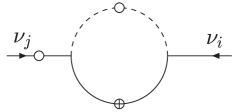
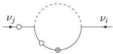
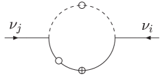
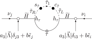
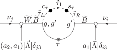
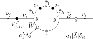
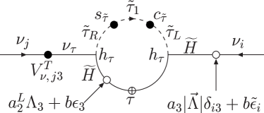
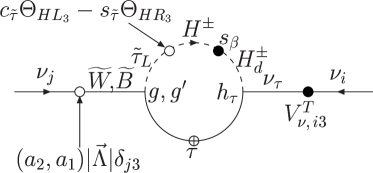
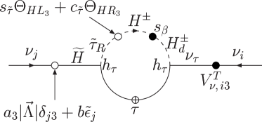
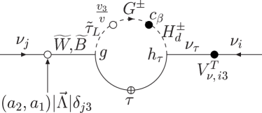
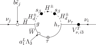
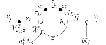
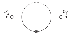
The relevant topologies for the one loop calculation of neutrino masses are then illustrated in Fig.1.
Refer to caption Refer to caption Refer to caption
Refer to caption Refer to caption
Figure 1: Topologies for neutrino self-energies in the BRpV supersymmetric model

Here our conventions are as follows: open circles with a cross inside indicate genuine mass insertions which flip chirality. On the other hand open circles without a cross correspond to small R-Parity violating projections, indicating how much of an Rp-even/odd mass eigenstate is present in a given Rp-odd/even weak eigenstate. Strictly speaking these projections are really coupling matrices attached to the vertices, and this is what appears in the numerical code. However, given the smallness of Rp-violating effects, the “insertion-method” proves to be a rather useful tool to develop an analytical perturbative expansion and to acquire some simple understanding of the results.

2.5 Bottom-sbottom loops

The simplest contribution to the radiatively induced neutrino mass arises from loops involving bottom quarks and squarks is given by Hirsch:2000ef

Π~ij(0)=Nc16π2r(ORjrbnb~OLirbnb~+OLjrbnb~ORirbnb~)mbB0(0,mb2,mr2)subscript~Π𝑖𝑗0subscript𝑁𝑐16superscript𝜋2subscript𝑟subscriptsuperscript𝑂𝑏𝑛~𝑏𝑅𝑗𝑟subscriptsuperscript𝑂𝑏𝑛~𝑏𝐿𝑖𝑟subscriptsuperscript𝑂𝑏𝑛~𝑏𝐿𝑗𝑟subscriptsuperscript𝑂𝑏𝑛~𝑏𝑅𝑖𝑟subscript𝑚𝑏subscript𝐵00superscriptsubscript𝑚𝑏2superscriptsubscript𝑚𝑟2\widetilde{\Pi}_{ij}(0)=-{{N_{c}}\over{16\pi^{2}}}\sum_{r}\left(O^{bn\tilde{b}}_{Rjr}O^{bn\tilde{b}}_{Lir}+O^{bn\tilde{b}}_{Ljr}O^{bn\tilde{b}}_{Rir}\right)m_{b}B_{0}(0,m_{b}^{2},m_{r}^{2}) (28)

B0(0,mb2,mr2)subscript𝐵00superscriptsubscript𝑚𝑏2superscriptsubscript𝑚𝑟2B_{0}(0,m_{b}^{2},m_{r}^{2}) is the usual Passarino-Veltman function Passarino:1978jh , FFLP . This contribution can be expressed as being proportional to the difference of two B0subscript𝐵0B_{0} functions,

ΔB0b~1b~2=B0(0,mb2,mb~12)B0(0,mb2,mb~22)Δsuperscriptsubscript𝐵0subscript~𝑏1subscript~𝑏2subscript𝐵00superscriptsubscript𝑚𝑏2superscriptsubscript𝑚subscript~𝑏12subscript𝐵00superscriptsubscript𝑚𝑏2superscriptsubscript𝑚subscript~𝑏22\Delta B_{0}^{\tilde{b}_{1}\tilde{b}_{2}}=B_{0}(0,m_{b}^{2},m_{\tilde{b}_{1}}^{2})-B_{0}(0,m_{b}^{2},m_{\tilde{b}_{2}}^{2}) (29)

as follows

ΔΠ~ij=Ncmb16π22sb~cb~hb2ΔB0b~1b~2[ϵ~iϵ~jμ2+a3b(ϵ~iδj3+ϵ~jδi3)|Λ|+(a32+aLaRhb2)δi3δj3|Λ|2]Δsubscript~Π𝑖𝑗subscript𝑁𝑐subscript𝑚𝑏16superscript𝜋22subscript𝑠~𝑏subscript𝑐~𝑏superscriptsubscript𝑏2Δsuperscriptsubscript𝐵0subscript~𝑏1subscript~𝑏2delimited-[]subscript~italic-ϵ𝑖subscript~italic-ϵ𝑗superscript𝜇2subscript𝑎3𝑏subscript~italic-ϵ𝑖subscript𝛿𝑗3subscript~italic-ϵ𝑗subscript𝛿𝑖3Λsuperscriptsubscript𝑎32subscript𝑎𝐿subscript𝑎𝑅subscriptsuperscript2𝑏subscript𝛿𝑖3subscript𝛿𝑗3superscriptΛ2\Delta\widetilde{\Pi}_{ij}=-{{N_{c}m_{b}}\over{16\pi^{2}}}2s_{\tilde{b}}c_{\tilde{b}}h_{b}^{2}\Delta B_{0}^{\tilde{b}_{1}\tilde{b}_{2}}\left[{{\tilde{\epsilon}_{i}\tilde{\epsilon}_{j}}\over{\mu^{2}}}+a_{3}b\left(\tilde{\epsilon}_{i}\delta_{j3}+\tilde{\epsilon}_{j}\delta_{i3}\right)|\vec{\Lambda}|+\left(a_{3}^{2}+\frac{a_{L}a_{R}}{h^{2}_{b}}\right)\delta_{i3}\delta_{j3}|\vec{\Lambda}|^{2}\right] (30)

where we have defined

aR=g2(13tWa1a2),aL=g223tWa1formulae-sequencesubscript𝑎𝑅𝑔213subscript𝑡𝑊subscript𝑎1subscript𝑎2subscript𝑎𝐿𝑔223subscript𝑡𝑊subscript𝑎1a_{R}={g\over{\sqrt{2}}}\left({1\over 3}t_{W}a_{1}-a_{2}\right)\,,\qquad a_{L}={g\over{\sqrt{2}}}\,{2\over 3}t_{W}a_{1} (31)

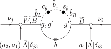
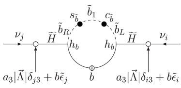
The different contributions can be understood as coming from the graphs corresponding to the first topology of Fig. 1. They have been depicted in more detail in Fig. 2,
Refer to caption Refer to caption
Figure 2: Bottom–Sbottom diagrams for solar neutrino mass in the BRpV model

where we have adopted the following conventions: a) as before, open circles correspond to small R-parity violating projections, indicating how much of a weak eigenstate is present in a given mass eigenstate, (b) full circles correspond to R-parity conserving projections and (c) open circles with a cross inside indicate genuine mass insertions which flip chirality.

The open and full circles should really appear at the vertices since the particles propagating in the loop are the mass eigenstates. We have however separated them to better identify the origin of the various terms. There is another set of graphs analogous to the previous ones which corresponds to the heavy sbottom. They are obtained from the previous graphs making the replacement b~1b~2subscript~𝑏1subscript~𝑏2\tilde{b}_{1}\rightarrow\tilde{b}_{2}, sb~cb~subscript𝑠~𝑏subscript𝑐~𝑏s_{\tilde{b}}\rightarrow c_{\tilde{b}} and cb~sb~subscript𝑐~𝑏subscript𝑠~𝑏c_{\tilde{b}}\rightarrow-s_{\tilde{b}}. Note that for all contributions to the 2×2222\times 2 submatrix corresponding to the light neutrinos the divergence from B0(0,mb2,mb~12)subscript𝐵00superscriptsubscript𝑚𝑏2superscriptsubscript𝑚subscript~𝑏12B_{0}(0,m_{b}^{2},m_{\tilde{b}_{1}}^{2}) is canceled by the divergence from B0(0,mb2,mb~22)subscript𝐵00superscriptsubscript𝑚𝑏2superscriptsubscript𝑚subscript~𝑏22B_{0}(0,m_{b}^{2},m_{\tilde{b}_{2}}^{2}), making finite the contribution from bottom-sbottom loops to this submatrix, as it should be, since the mass is fully “calculable”.

2.6 Charged Scalar-Charged Fermion Loops

Another contribution to the radiatively induced neutrino mass comes from charged-scalar/charged-fermion loops, given as Hirsch:2000ef

Π~ij(0)=116π2k,r(ORkjrcnsOLkircns+OLkjrcnsORkircns)mkB0(0,mk2,mr2)subscript~Π𝑖𝑗0116superscript𝜋2subscript𝑘𝑟subscriptsuperscript𝑂𝑐𝑛𝑠𝑅𝑘𝑗𝑟subscriptsuperscript𝑂𝑐𝑛𝑠𝐿𝑘𝑖𝑟subscriptsuperscript𝑂𝑐𝑛𝑠𝐿𝑘𝑗𝑟subscriptsuperscript𝑂𝑐𝑛𝑠𝑅𝑘𝑖𝑟subscript𝑚𝑘subscript𝐵00superscriptsubscript𝑚𝑘2superscriptsubscript𝑚𝑟2\widetilde{\Pi}_{ij}(0)=-{1\over{16\pi^{2}}}\sum_{k,r}\left(O^{cns}_{Rkjr}O^{cns}_{Lkir}+O^{cns}_{Lkjr}O^{cns}_{Rkir}\right)m_{k}B_{0}(0,m_{k}^{2},m_{r}^{2}) (32)

The structure of the contribution from charged Higgs/slepton loops is substantially more complex than that of the bottom-sbottom loop considered above. It can be expressed as

ΔΠ~ijΔsubscript~Π𝑖𝑗\displaystyle\hskip-8.53581pt\Delta\widetilde{\Pi}_{ij} =\displaystyle\hskip-5.69054pt=\hskip-5.69054pt mτ16π2[Cijτ~2τ~1ΔB0τ~2τ~1+CijH±τ~1ΔB0H±τ~1+CijH±τ~2ΔB0H±τ~2\displaystyle{{m_{\tau}}\over{16\pi^{2}}}\left[\vbox to18.0pt{}C_{ij}^{\tilde{\tau}_{2}\tilde{\tau}_{1}}\Delta B_{0}^{\tilde{\tau}_{2}\tilde{\tau}_{1}}+C_{ij}^{H^{\pm}\tilde{\tau}_{1}}\Delta B_{0}^{H^{\pm}\tilde{\tau}_{1}}+C_{ij}^{H^{\pm}\tilde{\tau}_{2}}\Delta B_{0}^{H^{\pm}\tilde{\tau}_{2}}\right. (33)
+CijH±L~1ΔB0H±L1+CijH±L~2ΔB0H±L2+CijG±L~1ΔB0G±L1superscriptsubscript𝐶𝑖𝑗superscript𝐻plus-or-minussubscript~𝐿1Δsuperscriptsubscript𝐵0superscript𝐻plus-or-minussubscript𝐿1superscriptsubscript𝐶𝑖𝑗superscript𝐻plus-or-minussubscript~𝐿2Δsuperscriptsubscript𝐵0superscript𝐻plus-or-minussubscript𝐿2superscriptsubscript𝐶𝑖𝑗superscript𝐺plus-or-minussubscript~𝐿1Δsuperscriptsubscript𝐵0superscript𝐺plus-or-minussubscript𝐿1\displaystyle\hskip 34.1433pt+C_{ij}^{H^{\pm}{\tilde{L}}_{1}}\Delta B_{0}^{H^{\pm}L_{1}}+C_{ij}^{H^{\pm}{\tilde{L}}_{2}}\Delta B_{0}^{H^{\pm}L_{2}}+C_{ij}^{G^{\pm}{\tilde{L}}_{1}}\Delta B_{0}^{G^{\pm}L_{1}}
+CijG±L~2ΔB0G±L2+CijG±τ~1τ~2ΔB0G±τ~1τ~2+CijG±H±τ~1τ~2ΔB0G±H±τ~1τ~2superscriptsubscript𝐶𝑖𝑗superscript𝐺plus-or-minussubscript~𝐿2Δsuperscriptsubscript𝐵0superscript𝐺plus-or-minussubscript𝐿2superscriptsubscript𝐶𝑖𝑗superscript𝐺plus-or-minussubscript~𝜏1subscript~𝜏2Δsuperscriptsubscript𝐵0superscript𝐺plus-or-minussubscript~𝜏1subscript~𝜏2superscriptsubscript𝐶𝑖𝑗superscript𝐺plus-or-minussuperscript𝐻plus-or-minussubscript~𝜏1subscript~𝜏2Δsuperscriptsubscript𝐵0superscript𝐺plus-or-minussuperscript𝐻plus-or-minussubscript~𝜏1subscript~𝜏2\displaystyle\hskip 34.1433pt+C_{ij}^{G^{\pm}{\tilde{L}}_{2}}\Delta B_{0}^{G^{\pm}L_{2}}+C_{ij}^{G^{\pm}\tilde{\tau}_{1}\tilde{\tau}_{2}}\Delta B_{0}^{G^{\pm}\tilde{\tau}_{1}\tilde{\tau}_{2}}+C_{ij}^{G^{\pm}H^{\pm}\tilde{\tau}_{1}\tilde{\tau}_{2}}\Delta B_{0}^{G^{\pm}H^{\pm}\tilde{\tau}_{1}\tilde{\tau}_{2}}
+(ij)]\displaystyle\hskip 34.1433pt\left.\vbox to14.0pt{}+(i\leftrightarrow j)\right]

where

ΔB0XYB0(0,mτ2,mX2)B0(0,mτ2,mY2);X,Y=(G±,H±,L1,L2,τ~1,τ~2)formulae-sequenceΔsuperscriptsubscript𝐵0𝑋𝑌subscript𝐵00superscriptsubscript𝑚𝜏2subscriptsuperscript𝑚2𝑋subscript𝐵00superscriptsubscript𝑚𝜏2superscriptsubscript𝑚𝑌2𝑋𝑌superscript𝐺plus-or-minussuperscript𝐻plus-or-minussubscript𝐿1subscript𝐿2subscript~𝜏1subscript~𝜏2\displaystyle\Delta B_{0}^{XY}\equiv B_{0}(0,m_{\tau}^{2},m^{2}_{X})-B_{0}(0,m_{\tau}^{2},m_{Y}^{2})\ ;\ X,Y=(G^{\pm},H^{\pm},L_{1},L_{2},\tilde{\tau}_{1},\tilde{\tau}_{2})
ΔB0G±τ~1τ~2cτ~2B0(0,mτ2,mτ~12)+sτ~2B0(0,mτ2,mτ~22)B0(0,mτ2,mG±2)Δsuperscriptsubscript𝐵0superscript𝐺plus-or-minussubscript~𝜏1subscript~𝜏2superscriptsubscript𝑐~𝜏2subscript𝐵00subscriptsuperscript𝑚2𝜏subscriptsuperscript𝑚2subscript~𝜏1superscriptsubscript𝑠~𝜏2subscript𝐵00subscriptsuperscript𝑚2𝜏subscriptsuperscript𝑚2subscript~𝜏2subscript𝐵00subscriptsuperscript𝑚2𝜏subscriptsuperscript𝑚2superscript𝐺plus-or-minus\displaystyle\Delta B_{0}^{G^{\pm}\tilde{\tau}_{1}\tilde{\tau}_{2}}\equiv c_{\tilde{\tau}}^{2}\,B_{0}(0,m^{2}_{\tau},m^{2}_{\tilde{\tau}_{1}})+s_{\tilde{\tau}}^{2}\,B_{0}(0,m^{2}_{\tau},m^{2}_{\tilde{\tau}_{2}})-B_{0}(0,m^{2}_{\tau},m^{2}_{G^{\pm}})
ΔB0G±H±τ~1τ~2cβ2B0(0,mτ2,mG±2)+sβ2B0(0,mτ2,mH±2)Δsuperscriptsubscript𝐵0superscript𝐺plus-or-minussuperscript𝐻plus-or-minussubscript~𝜏1subscript~𝜏2subscriptsuperscript𝑐2𝛽subscript𝐵00subscriptsuperscript𝑚2𝜏subscriptsuperscript𝑚2superscript𝐺plus-or-minussubscriptsuperscript𝑠2𝛽subscript𝐵00subscriptsuperscript𝑚2𝜏subscriptsuperscript𝑚2superscript𝐻plus-or-minus\displaystyle\Delta B_{0}^{G^{\pm}H^{\pm}\tilde{\tau}_{1}\tilde{\tau}_{2}}\equiv c^{2}_{\beta}\,B_{0}(0,m^{2}_{\tau},m^{2}_{G^{\pm}})+s^{2}_{\beta\,}B_{0}(0,m^{2}_{\tau},m^{2}_{H^{\pm}}) (34)
cτ~2B0(0,mτ2,mτ~12)sτ~2B0(0,mτ2,mτ~22)superscriptsubscript𝑐~𝜏2subscript𝐵00subscriptsuperscript𝑚2𝜏subscriptsuperscript𝑚2subscript~𝜏1superscriptsubscript𝑠~𝜏2subscript𝐵00subscriptsuperscript𝑚2𝜏subscriptsuperscript𝑚2subscript~𝜏2\displaystyle\hskip 73.97716pt-c_{\tilde{\tau}}^{2}\,B_{0}(0,m^{2}_{\tau},m^{2}_{\tilde{\tau}_{1}})-s_{\tilde{\tau}}^{2}\,B_{0}(0,m^{2}_{\tau},m^{2}_{\tilde{\tau}_{2}})

and

Cijτ~2τ~1=sτ~cτ~{2ga1|Λ|[gVν,j3Ta1LΛ312(ga2+ga1)|Λ|δj3]δi3\displaystyle C_{ij}^{\tilde{\tau}_{2}\tilde{\tau}_{1}}=s_{\tilde{\tau}}c_{\tilde{\tau}}\left\{\vbox to12.0pt{}\sqrt{2}g^{\prime}a_{1}|\vec{\Lambda}|\left[gV^{T}_{\nu,j3}a_{1}^{L}\Lambda_{3}-{\textstyle{1\over{\sqrt{2}}}}(ga_{2}+g^{\prime}a_{1})|\vec{\Lambda}|\delta_{j3}\right]\delta_{i3}\phantom{\hskip 85.35826pt}\right.
+hτ2(bϵ~i+a3|Λ|δi3cβv3vVν,i3T)[bϵ~j+a3|Λ|δj3Vν,j3T(a2LΛ3+bϵ3)]}\displaystyle\left.\hskip 62.59605pt\vbox to12.0pt{}+h_{\tau}^{2}\left(b\tilde{\epsilon}_{i}+a_{3}|\vec{\Lambda}|\delta_{i3}-c_{\beta}{\textstyle{{v_{3}}\over{v}}}V^{T}_{\nu,i3}\right)\left[b\tilde{\epsilon}_{j}+a_{3}|\vec{\Lambda}|\delta_{j3}-V^{T}_{\nu,j3}(a_{2}^{L}\Lambda_{3}+b\epsilon_{3})\right]\right\}
CijH±τ~1=sβΘHL3{cτ~hτVν,i3T[gVν,j3Ta1LΛ312(ga2+ga1)|Λ|δj3]\displaystyle C_{ij}^{H^{\pm}\tilde{\tau}_{1}}=-s_{\beta}\Theta_{HL_{3}}\left\{\vbox to12.0pt{}c_{\tilde{\tau}}h_{\tau}V^{T}_{\nu,i3}\Big{[}gV^{T}_{\nu,j3}a_{1}^{L}\Lambda_{3}-{\textstyle{1\over{\sqrt{2}}}}(ga_{2}+g^{\prime}a_{1})|\vec{\Lambda}|\delta_{j3}\Big{]}\right.
+sτ~hτ2Vν,i3T[bϵ~j+a3|Λ|δj3Vν,j3T(a2LΛ3+bϵ3)]}\displaystyle\left.\hskip 99.58464pt\vbox to12.0pt{}+s_{\tilde{\tau}}h_{\tau}^{2}V^{T}_{\nu,i3}\Big{[}b\tilde{\epsilon}_{j}+a_{3}|\vec{\Lambda}|\delta_{j3}-V^{T}_{\nu,j3}(a_{2}^{L}\Lambda_{3}+b\epsilon_{3})\Big{]}\right\}
CijH±τ~2=sβΘHR3{sτ~hτVν,i3T[gVν,j3Ta1LΛ312(ga2+ga1)|Λ|δj3]\displaystyle C_{ij}^{H^{\pm}\tilde{\tau}_{2}}=s_{\beta}\Theta_{HR_{3}}\left\{\vbox to12.0pt{}s_{\tilde{\tau}}h_{\tau}V^{T}_{\nu,i3}\Big{[}gV^{T}_{\nu,j3}a_{1}^{L}\Lambda_{3}-{\textstyle{1\over{\sqrt{2}}}}(ga_{2}+g^{\prime}a_{1})|\vec{\Lambda}|\delta_{j3}\Big{]}\right.
cτ~hτ2Vν,i3T[bϵ~j+a3|Λ|δj3Vν,j3T(a2LΛ3+bϵ3)]}\displaystyle\left.\hskip 85.35826pt\vbox to12.0pt{}-c_{\tilde{\tau}}h_{\tau}^{2}V^{T}_{\nu,i3}\Big{[}b\tilde{\epsilon}_{j}+a_{3}|\vec{\Lambda}|\delta_{j3}-V^{T}_{\nu,j3}(a_{2}^{L}\Lambda_{3}+b\epsilon_{3})\Big{]}\right\}
CijH±L1=sβΘ~HL1hτgVν,i3TVν,j1Ta1LΛ3superscriptsubscript𝐶𝑖𝑗superscript𝐻plus-or-minussubscript𝐿1subscript𝑠𝛽subscript~Θ𝐻subscript𝐿1subscript𝜏𝑔subscriptsuperscript𝑉𝑇𝜈𝑖3subscriptsuperscript𝑉𝑇𝜈𝑗1superscriptsubscript𝑎1𝐿subscriptΛ3\displaystyle C_{ij}^{H^{\pm}L_{1}}=-s_{\beta}\widetilde{\Theta}_{HL_{1}}\,h_{\tau}gV^{T}_{\nu,i3}V^{T}_{\nu,j1}a_{1}^{L}\Lambda_{3}
CijH±L2=sβΘ~HL2hτgVν,i3TVν,j2Ta1LΛ3superscriptsubscript𝐶𝑖𝑗superscript𝐻plus-or-minussubscript𝐿2subscript𝑠𝛽subscript~Θ𝐻subscript𝐿2subscript𝜏𝑔subscriptsuperscript𝑉𝑇𝜈𝑖3subscriptsuperscript𝑉𝑇𝜈𝑗2superscriptsubscript𝑎1𝐿subscriptΛ3\displaystyle C_{ij}^{H^{\pm}L_{2}}=-s_{\beta}\widetilde{\Theta}_{HL_{2}}\,h_{\tau}gV^{T}_{\nu,i3}V^{T}_{\nu,j2}a_{1}^{L}\Lambda_{3}
CijG±L1=cβv1vhτgVν,i3TVν,j1Ta1LΛ3superscriptsubscript𝐶𝑖𝑗superscript𝐺plus-or-minussubscript𝐿1subscript𝑐𝛽subscript𝑣1𝑣subscript𝜏𝑔subscriptsuperscript𝑉𝑇𝜈𝑖3subscriptsuperscript𝑉𝑇𝜈𝑗1superscriptsubscript𝑎1𝐿subscriptΛ3\displaystyle C_{ij}^{G^{\pm}L_{1}}=-c_{\beta}{{{v_{1}}\over v}}\,h_{\tau}gV^{T}_{\nu,i3}V^{T}_{\nu,j1}a_{1}^{L}\Lambda_{3} (35)
CijG±L2=cβv2vhτgVν,i3TVν,j2Ta1LΛ3superscriptsubscript𝐶𝑖𝑗superscript𝐺plus-or-minussubscript𝐿2subscript𝑐𝛽subscript𝑣2𝑣subscript𝜏𝑔subscriptsuperscript𝑉𝑇𝜈𝑖3subscriptsuperscript𝑉𝑇𝜈𝑗2superscriptsubscript𝑎1𝐿subscriptΛ3\displaystyle C_{ij}^{G^{\pm}L_{2}}=-c_{\beta}{{{v_{2}}\over v}}\,h_{\tau}gV^{T}_{\nu,i3}V^{T}_{\nu,j2}a_{1}^{L}\Lambda_{3}
CijG±τ~1τ~2=cβv3vhτVν,i3T[gVν,j3Ta1LΛ312(ga2+ga1)|Λ|δj3]superscriptsubscript𝐶𝑖𝑗superscript𝐺plus-or-minussubscript~𝜏1subscript~𝜏2subscript𝑐𝛽subscript𝑣3𝑣subscript𝜏subscriptsuperscript𝑉𝑇𝜈𝑖3delimited-[]𝑔subscriptsuperscript𝑉𝑇𝜈𝑗3superscriptsubscript𝑎1𝐿subscriptΛ312𝑔subscript𝑎2superscript𝑔subscript𝑎1Λsubscript𝛿𝑗3\displaystyle C_{ij}^{G^{\pm}\tilde{\tau}_{1}\tilde{\tau}_{2}}=c_{\beta}{{{v_{3}}\over v}}\,h_{\tau}V^{T}_{\nu,i3}\left[\vbox to12.0pt{}gV^{T}_{\nu,j3}a_{1}^{L}\Lambda_{3}-{{1\over{\sqrt{2}}}}(ga_{2}+g^{\prime}a_{1})|\vec{\Lambda}|\delta_{j3}\right]
CijG±H±τ~1τ~2=hτgϵ~iVν,i3Tba1LΛ3superscriptsubscript𝐶𝑖𝑗superscript𝐺plus-or-minussuperscript𝐻plus-or-minussubscript~𝜏1subscript~𝜏2subscript𝜏𝑔subscript~italic-ϵ𝑖subscriptsuperscript𝑉𝑇𝜈𝑖3𝑏superscriptsubscript𝑎1𝐿subscriptΛ3\displaystyle C_{ij}^{G^{\pm}H^{\pm}\tilde{\tau}_{1}\tilde{\tau}_{2}}=h_{\tau}g\tilde{\epsilon}_{i}V^{T}_{\nu,i3}ba_{1}^{L}\Lambda_{3}

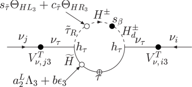
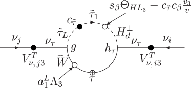
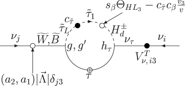
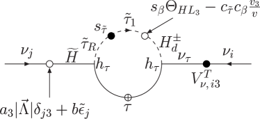
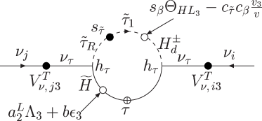
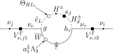
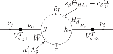
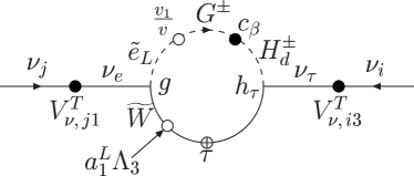
The result of Eq. (33) can be represented graphically for better understanding. The terms proportional to ΔB0τ~2τ~1Δsuperscriptsubscript𝐵0subscript~𝜏2subscript~𝜏1\Delta B_{0}^{\tilde{\tau}_{2}\tilde{\tau}_{1}} come from the graphs of Fig. 3. There is another set of four graphs corresponding to τ~2subscript~𝜏2\tilde{\tau}_{2}. These are found after making the replacements τ~1τ~2subscript~𝜏1subscript~𝜏2\tilde{\tau}_{1}\rightarrow\tilde{\tau}_{2}, sτ~cτ~subscript𝑠~𝜏subscript𝑐~𝜏s_{\tilde{\tau}}\rightarrow c_{\tilde{\tau}}, and cτ~sτ~subscript𝑐~𝜏subscript𝑠~𝜏c_{\tilde{\tau}}\rightarrow-s_{\tilde{\tau}}.

Refer to caption Refer to caption
Figure 3: Charged scalar contributions to solar neutrino masses in BRpV model: terms proportional to ΔB0τ~2τ~1Δsuperscriptsubscript𝐵0subscript~𝜏2subscript~𝜏1\Delta B_{0}^{\tilde{\tau}_{2}\tilde{\tau}_{1}}.

The diagrams in the first row are the ones that are equivalent to those in the bottom-sbottom loop. They have as characteristic feature the presence of two Rp-violating insertions (open circles) in the external legs. However, in contrast to the quark sector, R-parity violation can also appear in the charged internal lines running in the loops, since it occurs in the charged fermion sector. This explains the origin of the second row in Fig. 3. The presence of R-parity violating insertions in the internal lines of the second row in Fig. 3 correspond to the second topology in Fig. 1. The full diagrammatic explanation of the rest of the terms appearing in Eq. (33) is given in detail in Appendix  C.

3 Analytical versus Numerical results

In this section we will check the accuracy of the approximation formulas given in Sec. 2.5 and 2.6. We do this by comparing the results obtained with their use with a full numerical calculation of the one-loop contributions to the neutrino mass, whose details can be found in Ref. Hirsch:2000ef .

As will be explained in more detail below, the relative importance of the various loops depends on the - currently unknown - supersymmetric parameters. In order to reduce the number of free parameters in the following we will adopt the minimal constrained supergravity (mSUGRA) version of the MSSM. As a rule of thumb it can be said that the bottom-sbottom loop usually gives the main contribution to the neutrino mass matrix when the neutralino is the LSP. On the other hand, if the scalar tau is the LSP, both bottom-sbottom and charged scalar loops are of approximately comparable magnitudes.

We have therefore constructed two different random scans over SUSY parameter space. Both sets start with the following rather generous parameter ranges: M2subscript𝑀2M_{2} from [0,1.2] TeV, |μ|𝜇|\mu| from [0,2.5] TeV, m0subscript𝑚0m_{0} in the range [0,1.0] TeV, A0/m0subscript𝐴0subscript𝑚0A_{0}/m_{0} and B0/m0subscript𝐵0subscript𝑚0B_{0}/m_{0} [-3,3] and tanβ𝛽\tan\beta [2.5,10]. All randomly generated points were subsequently tested for consistency with the minimization (tadpole) conditions of the Higgs potential, as well as for phenomenological constraints from supersymmetric particle searches. We then selected points in which a) the lightest neutralino is the LSP (called set “Ntrl” in the following) or b) at least one of the charged sleptons was the LSP (called set “Stau” in the following). Note that in the Stau set m0<<M2much-less-thansubscript𝑚0subscript𝑀2m_{0}<<M_{2} and large μ𝜇\mu values are strongly preferred.

R-parity violating parameters are chosen in such a way that neutrino oscillation data are reproduced approximately. As discussed in the introduction, atmospheric neutrino experiments require a near-to-maximal atmospheric mixing angle θatm𝜃𝑎𝑡𝑚\theta{atm}, with Δm2atmΔsuperscript𝑚2𝑎𝑡𝑚\Delta m^{2}{atm} in the range given in Eq. (5). On the other hand reactor data constrain the electron-neutrino component in the third mass eigenstate to be small. And, finally, in combination with solar neutrino data, the KamLAND data require a θsol𝜃𝑠𝑜𝑙\theta{sol} in the range given in Eq. (2) with Δm2solΔsuperscript𝑚2𝑠𝑜𝑙\Delta m^{2}{sol} as given in Eq. (3). The latter ranges belong to the LMA-MSW region indicated by a solar-only global analysis of neutrino data given in Ref. Maltoni:2002ni . For completeness we also include the (pre-KamLAND) LOW and VAC-type solutions of the solar neutrino anomaly. In the following we will first discuss the bottom-sbottom and the charged scalar loops separately, before considering a calculation taking into account both loops in comparison to the full calculation.

3.1 Bottom-sbottom loop

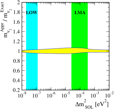
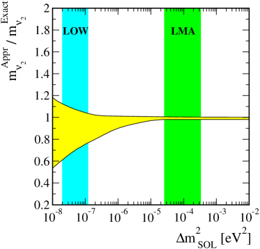
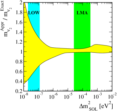
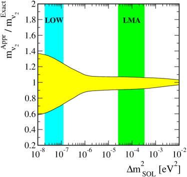
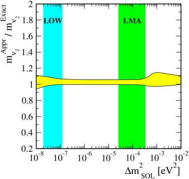
In Fig. 4 we show the ratio of the approximate-over-exact solar neutrino mass parameter mν2Appr/mν2exactsuperscriptsubscript𝑚subscript𝜈2𝐴𝑝𝑝𝑟superscriptsubscript𝑚subscript𝜈2𝑒𝑥𝑎𝑐𝑡m_{\nu_{2}}^{Appr}/m_{\nu_{2}}^{exact} versus Δm2solΔsuperscript𝑚2𝑠𝑜𝑙\Delta m^{2}{sol} for the case in which only the bottom-sbottom loop is taken into account, both in the approximate and in the exact calculation. The horizontal bands indicate attainable neutrino mass values when the parameters are scanned as indicated previously. As can be seen from the figure the approximate formula works quite well for points in both Ntrl and Stau sets, as long as the neutrino masses fall in the LMA-MSW range indicated by the right vertical bands. Note that the LMA-MSW and LOW bands indicated in the figure correspond to the full analysis of solar data only, presented in Ref. Maltoni:2002ni . The recent KamLAND reactor neutrino data rule out the LOW solution and restricts the LMA-MSW to somewhat narrower ranges indicated in Eq. (3). One finds that the mass values inferred from our present analytical approximation are always within 10 % or less of the exact numerical calculation of the bottom-sbottom loop. Larger deviations show up only in the Ntrl set, for very small neutrino masses, which we trace to the neglection of the 1-loop neutrino/neutralino mixing terms in our approximate treatment. Although not strictly ruled out by a solar-only global neutrino data analysis Maltoni:2002ni , these LOW and VAC-type solutions are now strongly disfavored by the latest KamLAND reactor neutrino data.
Refer to caption Refer to caption
Figure 4: Ratio mν2Appr/mν2exactsuperscriptsubscript𝑚subscript𝜈2𝐴𝑝𝑝𝑟superscriptsubscript𝑚subscript𝜈2𝑒𝑥𝑎𝑐𝑡m_{\nu_{2}}^{Appr}/m_{\nu_{2}}^{exact} versus Δm2solΔsuperscript𝑚2𝑠𝑜𝑙\Delta m^{2}{sol} in eV2𝑒superscript𝑉2eV^{2} for the sets Ntrl (left) and Stau (right), for a calculation involving only the bottom-sbottom loop. The vertical grid lines indicate the 90 % c.l. regions for the LOW and LMA solutions to the solar neutrino problem.

3.2 Charged scalar loop

Refer to caption Refer to caption
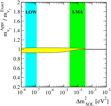
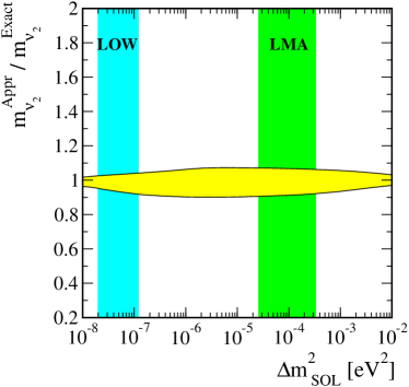
Figure 5: (mν2Appr/mν2exactsuperscriptsubscript𝑚subscript𝜈2𝐴𝑝𝑝𝑟superscriptsubscript𝑚subscript𝜈2𝑒𝑥𝑎𝑐𝑡m_{\nu_{2}}^{Appr}/m_{\nu_{2}}^{exact}) versus Δm2solΔsuperscript𝑚2𝑠𝑜𝑙\Delta m^{2}{sol} [eV2𝑒superscript𝑉2eV^{2}] for the sets Ntrl (left) and Stau (right), for a calculation involving only the charged scalar loop.

In Fig. 5 we show the ratio of the approximate-over-exact solar neutrino mass parameter mν2Appr/mν2exactsuperscriptsubscript𝑚subscript𝜈2𝐴𝑝𝑝𝑟superscriptsubscript𝑚subscript𝜈2𝑒𝑥𝑎𝑐𝑡m_{\nu_{2}}^{Appr}/m_{\nu_{2}}^{exact} plotted versus Δm2solΔsuperscript𝑚2𝑠𝑜𝑙\Delta m^{2}{sol}, for a calculation which takes into account only the charged scalar loop in both the approximate and the exact calculation. As can be seen from the figure the approximate formula is accurate for all points in the LMA-MSW region, indicated by the right vertical bands Maltoni:2002ni , both for the Stau and for the Ntrl sets. The only case where our analytic results gives a poorer approximation (to better than a factor-of-2) of the full numerical result is for the Ntrl set, when the neutrino mass falls in the LOW or VAC ranges, now strongly disfavored by the KamLAND results. We have checked numerically that for these very small neutrino masses all terms in eq. (33) are of approximately equal importance and there are significant cancellations among terms, which leads to a less reliable final result.

3.3 Comparison with full calculation
Refer to caption Refer to caption
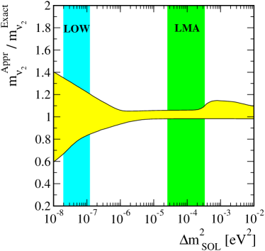
Figure 6: (mν2Appr/mν2exactsuperscriptsubscript𝑚subscript𝜈2𝐴𝑝𝑝𝑟superscriptsubscript𝑚subscript𝜈2𝑒𝑥𝑎𝑐𝑡m_{\nu_{2}}^{Appr}/m_{\nu_{2}}^{exact}) versus Δm2solΔsuperscript𝑚2𝑠𝑜𝑙\Delta m^{2}{sol} [eV2𝑒superscript𝑉2eV^{2}] for the set Ntrl (left) and the set Stau (right). mν2Apprsuperscriptsubscript𝑚subscript𝜈2𝐴𝑝𝑝𝑟m_{\nu_{2}}^{Appr} is the sum of the bottom-sbottom and charged scalar loops, while mν2exactsuperscriptsubscript𝑚subscript𝜈2𝑒𝑥𝑎𝑐𝑡m_{\nu_{2}}^{exact} is the numerical result for all loops. In case of LMA the approximation works always better than 10 %. For the LOW solution the typical error is of the order of 10 %, while in extreme cases errors up to 25 % can be found.

In supersymmetric models with mSUGRA-like boundary conditions the bottom-sbottom and the charged scalar loop usually give the most important contribution to the neutrino mass matrix. This is demonstrated in Fig. 6 (left) for the set Ntrl and in Fig. 6 (right) for the set Stau. In both figures we show the ratio of the approximate-over-exact solar neutrino mass parameter mν2Appr/mν2exactsuperscriptsubscript𝑚subscript𝜈2𝐴𝑝𝑝𝑟superscriptsubscript𝑚subscript𝜈2𝑒𝑥𝑎𝑐𝑡m_{\nu_{2}}^{Appr}/m_{\nu_{2}}^{exact} versus Δm2solΔsuperscript𝑚2𝑠𝑜𝑙\Delta m^{2}{sol} in eV2, where mν2Apprsuperscriptsubscript𝑚subscript𝜈2𝐴𝑝𝑝𝑟m_{\nu_{2}}^{Appr} is the approximate loop calculation involving the bottom-sbottom and the charged scalar loop, while mν2exactsuperscriptsubscript𝑚subscript𝜈2𝑒𝑥𝑎𝑐𝑡m_{\nu_{2}}^{exact} is the exact numerical computation taking into account all loops.

In the region of Δm2solΔsuperscript𝑚2𝑠𝑜𝑙\Delta m^{2}{sol} appropriate for the currently preferred LMA-MSW solution to the solar neutrino problem one finds that the approximate calculation reproduces the exact result better than 10 %. Only in the set Ntrl one finds larger deviations, up to 25 % in extreme cases, when Δm2solΔsuperscript𝑚2𝑠𝑜𝑙\Delta m^{2}{sol} lies in the LOW region, strongly disfavored by KamLAND. This is due to the larger errors in the bottom-sbottom calculation in this set for small neutrino masses as discussed above.

4 Simplified approximation formulas

4.1 The solar mass

First we note that for nearly all points in our random sets we find that mν2mν3much-less-thansubscript𝑚subscript𝜈2subscript𝑚subscript𝜈3m_{\nu_{2}}\ll m_{\nu_{3}}. In other words, bilinear R-parity breaking favors a hierarchical neutrino spectrum. Moreover, we have found numerically that the terms proportional to ϵ~i×ϵ~jsubscript~italic-ϵ𝑖subscript~italic-ϵ𝑗{\tilde{\epsilon}_{i}}\times{\tilde{\epsilon}_{j}} in the self energies in Eq. (30) give the most important contribution to mν2subscript𝑚subscript𝜈2m_{\nu_{2}} in the bottom-sbottom loop calculation in most points of our sets. If these terms are dominant one can find a very simple approximation for the bottom-sbottom loop contribution to mν2subscript𝑚subscript𝜈2m_{\nu_{2}}. It is given by

mν2316π2sin(2θb~)mbΔB0τ~2τ~1(ϵ~12+ϵ~22)μ2similar-to-or-equalssubscript𝑚subscript𝜈2316superscript𝜋22subscript𝜃~𝑏subscript𝑚𝑏Δsuperscriptsubscript𝐵0subscript~𝜏2subscript~𝜏1superscriptsubscript~italic-ϵ12superscriptsubscript~italic-ϵ22superscript𝜇2m_{\nu_{2}}\simeq\frac{3}{16\pi^{2}}\sin(2\theta_{\tilde{b}})m_{b}\Delta B_{0}^{\tilde{\tau}_{2}\tilde{\tau}_{1}}\ \frac{({\tilde{\epsilon}}_{1}^{2}+{\tilde{\epsilon}}_{2}^{2})}{\mu^{2}} (36)

We have checked numerically that Eq. (36) reproduces the result of the full approximative formula to high accuracy if mν20.3mν3subscript𝑚subscript𝜈20.3subscript𝑚subscript𝜈3m_{\nu_{2}}\leq 0.3m_{\nu_{3}} . Note also that Eq. (36) holds only if the 1-loop contributions to the neutrino mass matrix are smaller than the tree-level one. This condition requires that |ϵ|2/|Λ|1superscriptitalic-ϵ2Λ1|{\vec{\epsilon}}|^{2}/|\Lambda|\leq 1 approximately, i.e. the bilinear parameters ϵisubscriptitalic-ϵ𝑖\epsilon_{i} must be suppressed with respect to μ𝜇\mu. Note that such a suppression could, in principle, be motivated by suitable flavour symmetries Mira:2000gg .

Due to the more complicated structure of the charged scalar loop it is not possible to give a simple equation for mν2subscript𝑚subscript𝜈2m_{\nu_{2}} similar to Eq. (36) for the bottom-sbottom loop. However, for mν2subscript𝑚subscript𝜈2m_{\nu_{2}} larger than (few) ×104absentsuperscript104\times 10^{-4} we have found that the most important contributions to the charged scalar loop are the terms proportional to ΔB0τ~2τ~1Δsuperscriptsubscript𝐵0subscript~𝜏2subscript~𝜏1\Delta B_{0}^{\tilde{\tau}_{2}\tilde{\tau}_{1}}, ΔB0H±τ~1Δsuperscriptsubscript𝐵0superscript𝐻plus-or-minussubscript~𝜏1\Delta B_{0}^{H^{\pm}\tilde{\tau}_{1}} and ΔB0H±τ~2Δsuperscriptsubscript𝐵0superscript𝐻plus-or-minussubscript~𝜏2\Delta B_{0}^{H^{\pm}\tilde{\tau}_{2}} in Eq. (33). We note in passing that Eq. (36), with appropriate replacements, allows us to estimate the typical contributions to the charged scalar loop within a factor of 3similar-toabsent3\sim 3. However, such an estimate will be biased toward too small (large) mν2subscript𝑚subscript𝜈2m_{\nu_{2}} for scalar tau (neutralino) LSPs.

Refer to caption Refer to caption
Figure 7: (mν2Appr/mν2exactsuperscriptsubscript𝑚subscript𝜈2𝐴𝑝𝑝𝑟superscriptsubscript𝑚subscript𝜈2𝑒𝑥𝑎𝑐𝑡m_{\nu_{2}}^{Appr}/m_{\nu_{2}}^{exact}) versus Δm2solΔsuperscript𝑚2𝑠𝑜𝑙\Delta m^{2}{sol} [eV2𝑒superscript𝑉2eV^{2}] for the set Ntrl (left) and Stau (right). Shown is the result of the simplified approximation formula in Eq. (36) for the sbottom-bottom loop and taking into account only coefficients CH±τ~2subscript𝐶superscript𝐻plus-or-minussubscript~𝜏2C_{H^{\pm}\tilde{\tau}_{2}}, CH±τ~1subscript𝐶superscript𝐻plus-or-minussubscript~𝜏1C_{H^{\pm}\tilde{\tau}_{1}} and Cτ~2τ~1subscript𝐶subscript~𝜏2subscript~𝜏1C_{\tilde{\tau}_{2}\tilde{\tau}_{1}} in the charged scalar loop.

In Fig. (7) we show a comparison of our simplified approximation formula, including the simple form of the sbottom-bottom loop and the three most important coefficients for the charged scalar loop, as discussed above, to the full numerical calculation including all loops. As one can see, even the simplified version of our formula works surprisingly well in the LMA-MSW regime, although the agreement with the full calculation is now less good for the LOW region, as could have been expected from the results discussed previously.

4.2 The solar mixing angle

In the basis where the tree-level neutrino mass matrix is diagonal the mass matrix at one–loop level can be written as

m~ν=Vν(0)TmνVν(0)=(c1ϵ~1ϵ~1c1ϵ~1ϵ~2c1ϵ~1ϵ~3c1ϵ~2ϵ~1c1ϵ~2ϵ~2c1ϵ~2ϵ~3c1ϵ~3ϵ~1c1ϵ~3ϵ~2c0|Λ|2+c1ϵ~3ϵ~3)+subscript~𝑚𝜈superscriptsubscript𝑉𝜈0𝑇subscript𝑚𝜈superscriptsubscript𝑉𝜈0subscript𝑐1subscript~italic-ϵ1subscript~italic-ϵ1subscript𝑐1subscript~italic-ϵ1subscript~italic-ϵ2subscript𝑐1subscript~italic-ϵ1subscript~italic-ϵ3subscript𝑐1subscript~italic-ϵ2subscript~italic-ϵ1subscript𝑐1subscript~italic-ϵ2subscript~italic-ϵ2subscript𝑐1subscript~italic-ϵ2subscript~italic-ϵ3subscript𝑐1subscript~italic-ϵ3subscript~italic-ϵ1subscript𝑐1subscript~italic-ϵ3subscript~italic-ϵ2subscript𝑐0superscriptΛ2subscript𝑐1subscript~italic-ϵ3subscript~italic-ϵ3\displaystyle\widetilde{m}_{\nu}=V_{\nu}^{(0)T}m_{\nu}V_{\nu}^{(0)}=\left(\begin{array}[]{ccc}c_{1}\widetilde{\epsilon}_{1}\widetilde{\epsilon}_{1}&c_{1}\widetilde{\epsilon}_{1}\widetilde{\epsilon}_{2}&c_{1}\widetilde{\epsilon}_{1}\widetilde{\epsilon}_{3}\\ c_{1}\widetilde{\epsilon}_{2}\widetilde{\epsilon}_{1}&c_{1}\widetilde{\epsilon}_{2}\widetilde{\epsilon}_{2}&c_{1}\widetilde{\epsilon}_{2}\widetilde{\epsilon}_{3}\\ c_{1}\widetilde{\epsilon}_{3}\widetilde{\epsilon}_{1}&c_{1}\widetilde{\epsilon}_{3}\widetilde{\epsilon}_{2}&c_{0}|\vec{\Lambda}|^{2}+c_{1}\widetilde{\epsilon}_{3}\widetilde{\epsilon}_{3}\end{array}\right)+\cdots (40)

where the ϵ~isubscript~italic-ϵ𝑖\widetilde{\epsilon}_{i} were defined before in Eq. (2.2). Coefficients c0subscript𝑐0c_{0} and c1subscript𝑐1c_{1} contain couplings and supersymmetric masses. Since they cancel in the final expression for the angle their exact definition is not necessary in the following. Dots stand for other terms which we will assume to be less important in the following, see the discussion at the end of this subsection. This matrix can be diagonalized approximately under the condition

xc1|ϵ~|2c0|Λ|21𝑥subscript𝑐1superscript~italic-ϵ2subscript𝑐0superscriptΛ2much-less-than1\displaystyle x\equiv\frac{c_{1}|\vec{\widetilde{\epsilon}}|^{2}}{c_{0}|\vec{\Lambda}|^{2}}\ll 1 (41)

i.e. if the 1-loop contribution to the neutrino mass matrix is smaller than the tree-level contribution, as also discussed above for Eq. (36). Then

m~ν=c0|Λ|2(xϵ~1ϵ~1|ϵ~|2xϵ~1ϵ~2|ϵ~|2xϵ~1ϵ~3|ϵ~|2xϵ~2ϵ~1|ϵ~|2xϵ~2ϵ~2|ϵ~|2xϵ~2ϵ~3|ϵ~|2xϵ~3ϵ~1|ϵ~|2xϵ~3ϵ~2|ϵ~|21+xϵ~3ϵ~3|ϵ~|2)\displaystyle\widetilde{m}_{\nu}=c_{0}|\vec{\Lambda}|^{2}\left(\begin{array}[]{ccc}\displaystyle x\,\frac{\widetilde{\epsilon}_{1}\widetilde{\epsilon}_{1}}{|\vec{\widetilde{\epsilon}|^{2}}}&\displaystyle x\,\frac{\widetilde{\epsilon}_{1}\widetilde{\epsilon}_{2}}{|\vec{\widetilde{\epsilon}|^{2}}}&\displaystyle x\,\frac{\widetilde{\epsilon}_{1}\widetilde{\epsilon}_{3}}{|\vec{\widetilde{\epsilon}|^{2}}}\\[11.38109pt] \displaystyle x\,\frac{\widetilde{\epsilon}_{2}\widetilde{\epsilon}_{1}}{|\vec{\widetilde{\epsilon}|^{2}}}&\displaystyle x\,\frac{\widetilde{\epsilon}_{2}\widetilde{\epsilon}_{2}}{|\vec{\widetilde{\epsilon}|^{2}}}&\displaystyle x\,\frac{\widetilde{\epsilon}_{2}\widetilde{\epsilon}_{3}}{|\vec{\widetilde{\epsilon}|^{2}}}\\[11.38109pt] \displaystyle x\,\frac{\widetilde{\epsilon}_{3}\widetilde{\epsilon}_{1}}{|\vec{\widetilde{\epsilon}|^{2}}}&\displaystyle x\,\frac{\widetilde{\epsilon}_{3}\widetilde{\epsilon}_{2}}{|\vec{\widetilde{\epsilon}|^{2}}}&\displaystyle 1+x\,\frac{\widetilde{\epsilon}_{3}\widetilde{\epsilon}_{3}}{|\vec{\widetilde{\epsilon}|^{2}}}\end{array}\right) (45)

We now calculate the eigenvalues and eigenvectors of this matrix as series expansions in the small x𝑥x parameter. For the eigenvalues we get

m1subscript𝑚1\displaystyle m_{1} =\displaystyle= 00\displaystyle 0
m2subscript𝑚2\displaystyle m_{2} =\displaystyle= xc0|Λ|2|ϵ~|2+𝒪(x2)=c1(ϵ~12+ϵ~22)+𝒪(x2)\displaystyle x\,c_{0}\frac{|\vec{\Lambda}|^{2}}{|\vec{\widetilde{\epsilon}|^{2}}}+\mathcal{O}(x^{2})=c_{1}\left(\widetilde{\epsilon}_{1}^{2}+\widetilde{\epsilon}_{2}^{2}\right)+\mathcal{O}(x^{2}) (46)
m3subscript𝑚3\displaystyle m_{3} =\displaystyle= c0|Λ|2+c1ϵ~32+𝒪(x2)subscript𝑐0superscriptΛ2subscript𝑐1superscriptsubscript~italic-ϵ32𝒪superscript𝑥2\displaystyle c_{0}|\vec{\Lambda}|^{2}+c_{1}\widetilde{\epsilon}_{3}^{2}+\mathcal{O}(x^{2})

and for the first two eigenvalues (the third can also be easily obtained but it will not be necessary for the discussion of the solar mixing angle),

e1subscript𝑒1\displaystyle e_{1} =\displaystyle= (ϵ~2ϵ~1ϵ~12ϵ~12+ϵ~22,ϵ~12ϵ~12+ϵ~22, 0)subscript~italic-ϵ2subscript~italic-ϵ1superscriptsubscript~italic-ϵ12superscriptsubscript~italic-ϵ12superscriptsubscript~italic-ϵ22superscriptsubscript~italic-ϵ12superscriptsubscript~italic-ϵ12superscriptsubscript~italic-ϵ22 0\displaystyle\left(-\frac{\widetilde{\epsilon}_{2}}{\widetilde{\epsilon}_{1}}\,\sqrt{\frac{\widetilde{\epsilon}_{1}^{2}}{\widetilde{\epsilon}_{1}^{2}+\widetilde{\epsilon}_{2}^{2}}},\ \sqrt{\frac{\widetilde{\epsilon}_{1}^{2}}{\widetilde{\epsilon}_{1}^{2}+\widetilde{\epsilon}_{2}^{2}}},\ 0\right)
e2subscript𝑒2\displaystyle e_{2} =\displaystyle= (e2,1,e2,2,e2,3)subscript𝑒21subscript𝑒22subscript𝑒23\displaystyle\left(e_{2,1},e_{2,2},e_{2,3}\right) (47)

where up to 𝒪(x2)𝒪superscript𝑥2\mathcal{O}(x^{2}) we have,

e2,1subscript𝑒21\displaystyle e_{2,1} =\displaystyle= ϵ~1ϵ~3ϵ~32(ϵ~12+ϵ~22)+12ϵ~1ϵ~3ϵ~32(ϵ~12+ϵ~22)|ϵ~|4x2+𝒪(x3)\displaystyle-\frac{\widetilde{\epsilon}_{1}\widetilde{\epsilon}_{3}}{\sqrt{\widetilde{\epsilon}_{3}^{2}(\widetilde{\epsilon}_{1}^{2}+\widetilde{\epsilon}_{2}^{2})}}+\frac{1}{2}\,\frac{\widetilde{\epsilon}_{1}\widetilde{\epsilon}_{3}\sqrt{\widetilde{\epsilon}_{3}^{2}(\widetilde{\epsilon}_{1}^{2}+\widetilde{\epsilon}_{2}^{2})}}{|\vec{\widetilde{\epsilon}|^{4}}}\ x^{2}+\mathcal{O}(x^{3})
e2,2subscript𝑒22\displaystyle e_{2,2} =\displaystyle= ϵ~2ϵ~3ϵ~32(ϵ~12+ϵ~22)+12ϵ~2ϵ~3ϵ~32(ϵ~12+ϵ~22)|ϵ~|4x2+𝒪(x3)\displaystyle-\frac{\widetilde{\epsilon}_{2}\widetilde{\epsilon}_{3}}{\sqrt{\widetilde{\epsilon}_{3}^{2}(\widetilde{\epsilon}_{1}^{2}+\widetilde{\epsilon}_{2}^{2})}}+\frac{1}{2}\,\frac{\widetilde{\epsilon}_{2}\widetilde{\epsilon}_{3}\sqrt{\widetilde{\epsilon}_{3}^{2}(\widetilde{\epsilon}_{1}^{2}+\widetilde{\epsilon}_{2}^{2})}}{|\vec{\widetilde{\epsilon}|^{4}}}\ x^{2}+\mathcal{O}(x^{3}) (48)
e2,3subscript𝑒23\displaystyle e_{2,3} =\displaystyle= ϵ~32(ϵ~12+ϵ~22)|ϵ~|2x+(ϵ~12+ϵ~22ϵ~32)ϵ~32(ϵ~12+ϵ~22)|ϵ~|4x2+𝒪(x3)\displaystyle\frac{\sqrt{\widetilde{\epsilon}_{3}^{2}(\widetilde{\epsilon}_{1}^{2}+\widetilde{\epsilon}_{2}^{2})}}{|\vec{\widetilde{\epsilon}|^{2}}}\ x+\frac{\left(\widetilde{\epsilon}_{1}^{2}+\widetilde{\epsilon}_{2}^{2}-\widetilde{\epsilon}_{3}^{2}\right)\sqrt{\widetilde{\epsilon}_{3}^{2}(\widetilde{\epsilon}_{1}^{2}+\widetilde{\epsilon}_{2}^{2})}}{|\vec{\widetilde{\epsilon}|^{4}}}\ x^{2}+\mathcal{O}(x^{3})

Knowing the eigenvectors we can write down the rotation matrix that diagonalizes m~νsubscript~𝑚𝜈\widetilde{m}_{\nu},

V~νTm~νV~ν=diag(m1,m2,m3)superscriptsubscript~𝑉𝜈𝑇subscript~𝑚𝜈subscript~𝑉𝜈diagsubscript𝑚1subscript𝑚2subscript𝑚3\displaystyle\widetilde{V}_{\nu}^{T}\widetilde{m}_{\nu}\widetilde{V}_{\nu}=\hbox{diag}(m_{1},m_{2},m_{3}) (49)

where

V~νT=(e1,1e1,2e1,3e2,1e2,2e2,3e3,1e3,2e3,3)superscriptsubscript~𝑉𝜈𝑇subscript𝑒11subscript𝑒12subscript𝑒13subscript𝑒21subscript𝑒22subscript𝑒23subscript𝑒31subscript𝑒32subscript𝑒33\displaystyle\widetilde{V}_{\nu}^{T}=\left(\begin{array}[]{ccc}e_{1,1}&e_{1,2}&e_{1,3}\\ e_{2,1}&e_{2,2}&e_{2,3}\\ e_{3,1}&e_{3,2}&e_{3,3}\end{array}\right) (53)

The neutrino mixing matrix is then given by

U=(VνTV~νT)T𝑈superscriptsuperscriptsubscript𝑉𝜈𝑇superscriptsubscript~𝑉𝜈𝑇𝑇\displaystyle U=\left(V_{\nu}^{T}\widetilde{V}_{\nu}^{T}\right)^{T} (54)

Using the fact that Ue3subscript𝑈𝑒3U_{e3} has to be small one can get the following expression for the solar mixing angle:

tan2θsol=Ue22Ue12superscript2𝜃𝑠𝑜𝑙superscriptsubscript𝑈𝑒22superscriptsubscript𝑈𝑒12\displaystyle\tan^{2}\theta{sol}=\frac{U_{e2}^{2}}{U_{e1}^{2}} (55)

Now using the Eqs. (53), (4.2) and substituting in Eq. (54) we obtain the very simple expression for the solar mixing angle,

tan2θsol=ϵ~12ϵ~22superscript2𝜃𝑠𝑜𝑙superscriptsubscript~italic-ϵ12superscriptsubscript~italic-ϵ22\displaystyle\tan^{2}\theta{sol}=\frac{\widetilde{\epsilon}_{1}^{2}}{\widetilde{\epsilon}_{2}^{2}} (56)

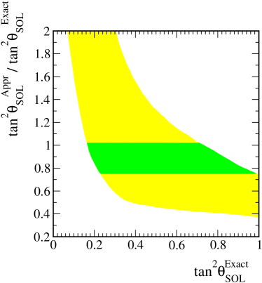
This formula is a very good approximation if the one–loop matrix has the structure ϵi×ϵjsubscriptitalic-ϵ𝑖subscriptitalic-ϵ𝑗\epsilon_{i}\times\epsilon_{j}, as is the case of the bottom-sbottom loop (and, to a lesser extend also for the charged scalar loop, which has one coefficient with the same index structure), and if mν3mν2much-greater-thansubscript𝑚subscript𝜈3subscript𝑚subscript𝜈2m_{\nu_{3}}\gg m_{\nu_{2}} . This is illustrated in Fig. 8.

In the left panel we show a calculation comparing for all points in the set Ntrl the approximate to the exact solar angle, while the right panel shows a subset of points using the cut sin(2θb~)ΔB0τ~2τ~1>0.022subscript𝜃~𝑏Δsuperscriptsubscript𝐵0subscript~𝜏2subscript~𝜏10.02\sin(2\theta_{\tilde{b}})\Delta B_{0}^{\tilde{\tau}_{2}\tilde{\tau}_{1}}>0.02. Note that this cut is designed such as to prefer points in which there is a sizeable contribution to the full 1-loop neutrino mass due to the bottom-sbottom loop. For points in which the charged scalar loop dominates eq. (56) gives only a factor-of-two estimate of the true solar angle.

Note finally that eq. (56) will fail completely, if ΛμΛτsubscriptΛ𝜇subscriptΛ𝜏\Lambda_{\mu}\equiv\Lambda_{\tau} and ϵμϵτsubscriptitalic-ϵ𝜇subscriptitalic-ϵ𝜏\epsilon_{\mu}\equiv\epsilon_{\tau}, since then ϵ~22=0superscriptsubscript~italic-ϵ220{\widetilde{\epsilon}_{2}^{2}}=0, see Eq. (2.2). This is the origin of the “sign condition” discussed in Hirsch:2000ef .
Refer to caption Refer to caption
Figure 8: (tan2θsolAppr/tan2θsolexactsuperscript2𝜃𝑠𝑜superscript𝑙𝐴𝑝𝑝𝑟superscript2𝜃𝑠𝑜superscript𝑙𝑒𝑥𝑎𝑐𝑡{\tan^{2}\theta{sol}}^{Appr}/{\tan^{2}\theta{sol}}^{exact}) versus tan2θsolexactsuperscript2𝜃𝑠𝑜superscript𝑙𝑒𝑥𝑎𝑐𝑡{\tan^{2}\theta{sol}}^{exact}. On the left panel the darker region contains over 90% of the points in our sample. In the right panel the points in the region shown satisfy the cut sin(2θb~)ΔB0τ~2τ~1>0.022subscript𝜃~𝑏Δsuperscriptsubscript𝐵0subscript~𝜏2subscript~𝜏10.02\sin(2\theta_{\tilde{b}})\Delta B_{0}^{\tilde{\tau}_{2}\tilde{\tau}_{1}}>0.02 .

5 Discussion and conclusions

We have presented an approximate calculation of the neutrino mass matrix at one-loop in supersymmetry with bilinearly broken R-parity. The method is based on a systematic perturbative expansion of R-parity violating vertices to leading order. We have identified the bottom-sbottom and the charged scalar loop as the most important ones, at least in supersymmetric models with mSUGRA-like boundary conditions. Taking into account only these loops, we have given explicit formulas and discussed their validity as well as the accuracy with which they describe solar neutrino mass and mixing parameters. This was done by comparing our analytical results to the exact numerical calculation. We have found that for the case of the large mixing MSW solution our formulas - even within the simplified form Eq. (36) and Eq. (56) - yield good agreement with the full numerical calculation, but are much simpler to implement than the full numerical one-loop calculation. The only solar neutrino “solutions” for which our analytical approximation is less accurate are those that are now ruled out by the recent reactor neutrino data from KamLAND.

Let us finally discuss some possible caveats to the success of our approximate treatment. One is the assumption that supersymmetry breaking mass terms are flavour diagonal, which we have adopted, motivated by constraints from flavour changing processes. Although such terms could be included into our approximate treatment, we have not done so, mainly due to the fact that the resulting formulas would be much more complicated and, therefore, of very limited practical use. A second concern is that our sample points were all generated using mSugra assumptions for the soft breaking masses. Clearly there are other possibilities to break supersymmetry and even though we expect that the bottom-sbottom loop and the charged scalar loop will still be well described by our approximation formulas, other loops, which we didn’t take into account, might be more important than what we have found in our data sets.

Acknowledgements

This work was supported by Spanish grant BFM2002-00345, by the European Commission RTN grant HPRN-CT-2000-00148 and the ESF Neutrino Astrophysics Network. M. H. is supported by a Spanish MCyT Ramon y Cajal contract. W. P. is supported by the ’Erwin Schrödinger fellowship No. J2095’ of the ‘Fonds zur Förderung der wissenschaftlichen Forschung’ of Austria FWF and partly by the Swiss ‘Nationalfonds’. M.A.D. was supported by Conicyt grant No. 1010974. J.R. was partly supported by the fellowship SFRH/BSAB/269/2002 from FCT (Portugal) with funds from the EU.

Appendix A Rotation Matrices

In the basis (Hd+,Hu+,e~L+,μ~L+,τ~L+,e~R+,μ~R+,τ~R+)superscriptsubscript𝐻𝑑superscriptsubscript𝐻𝑢superscriptsubscript~𝑒𝐿superscriptsubscript~𝜇𝐿superscriptsubscript~𝜏𝐿superscriptsubscript~𝑒𝑅superscriptsubscript~𝜇𝑅superscriptsubscript~𝜏𝑅(H_{d}^{+},H_{u}^{+},\widetilde{e}_{L}^{+},\widetilde{\mu}_{L}^{+},\widetilde{\tau}_{L}^{+},\widetilde{e}_{R}^{+},\widetilde{\mu}_{R}^{+},\widetilde{\tau}_{R}^{+}), one can write, to first order in R-parity violating parameters, the Goldstone rotation matrix as

𝐑G=[cβsβv1/vv2/vv3/v000sβcβ000000cβv1/vsβv1/v100000cβv2/vsβv2/v010000cβv3/vsβv3/v001000000001000000001000000001]subscript𝐑𝐺delimited-[]matrixsubscript𝑐𝛽subscript𝑠𝛽subscript𝑣1𝑣subscript𝑣2𝑣subscript𝑣3𝑣000subscript𝑠𝛽subscript𝑐𝛽000000subscript𝑐𝛽subscript𝑣1𝑣subscript𝑠𝛽subscript𝑣1𝑣100000subscript𝑐𝛽subscript𝑣2𝑣subscript𝑠𝛽subscript𝑣2𝑣010000subscript𝑐𝛽subscript𝑣3𝑣subscript𝑠𝛽subscript𝑣3𝑣001000000001000000001000000001{\bf R}_{G}=\left[\matrix{c_{\beta}&-s_{\beta}&v_{1}/v&v_{2}/v&v_{3}/v&0&0&0\cr s_{\beta}&c_{\beta}&0&0&0&0&0&0\cr-c_{\beta}v_{1}/v&s_{\beta}v_{1}/v&1&0&0&0&0&0\cr-c_{\beta}v_{2}/v&s_{\beta}v_{2}/v&0&1&0&0&0&0\cr-c_{\beta}v_{3}/v&s_{\beta}v_{3}/v&0&0&1&0&0&0\cr 0&0&0&0&0&1&0&0\cr 0&0&0&0&0&0&1&0\cr 0&0&0&0&0&0&0&1\cr}\right] (57)

where v2=vd2+vu2superscript𝑣2superscriptsubscript𝑣𝑑2superscriptsubscript𝑣𝑢2v^{2}=v_{d}^{2}+v_{u}^{2} to this order, and tanβ=vu/vd𝛽subscript𝑣𝑢subscript𝑣𝑑\tan\beta=v_{u}/v_{d}, as usual. We have also used the shorthand notation cβ(sβ)=cosβ(sinβ)subscript𝑐𝛽subscript𝑠𝛽𝛽𝛽c_{\beta}(s_{\beta})=\cos\beta(\sin\beta).

Neglecting the electron and muon Yukawa couplings, the rotation that diagonalizes the sleptons at tree level is given by (in the same basis as above)

𝐑τ~=[100000000100000000100000000100000000cτ~00sτ~00000100000000100000sτ~00cτ~]subscript𝐑~𝜏delimited-[]matrix100000000100000000100000000100000000subscript𝑐~𝜏00subscript𝑠~𝜏00000100000000100000subscript𝑠~𝜏00subscript𝑐~𝜏{\bf R}_{\tilde{\tau}}=\left[\matrix{1&0&0&0&0&0&0&0\cr 0&1&0&0&0&0&0&0\cr 0&0&1&0&0&0&0&0\cr 0&0&0&1&0&0&0&0\cr 0&0&0&0&c_{\tilde{\tau}}&0&0&s_{\tilde{\tau}}\cr 0&0&0&0&0&1&0&0\cr 0&0&0&0&0&0&1&0\cr 0&0&0&0&-s_{\tilde{\tau}}&0&0&c_{\tilde{\tau}}\cr}\right] (58)

After the rotations 𝐑τ~𝐑Gsubscript𝐑~𝜏subscript𝐑𝐺{\bf R}_{\tilde{\tau}}{\bf R}_{G} are performed, the charged scalar mass matrix is diagonalized up to small R-parity violating entries. In the approximation where there is no intergenerational mixing and hμhe0subscript𝜇subscript𝑒0h_{\mu}\approx h_{e}\approx 0, these are

𝚫𝐌𝐒±𝟐τ~=[0000000000X~HL1X~HL2X~HL300X~HR30X~HL10000000X~HL20000000X~HL300000000000000000000000X~HR3000000]𝚫subscriptsubscriptsuperscript𝐌2superscript𝐒plus-or-minus~𝜏delimited-[]matrix0000000000subscript~𝑋𝐻subscript𝐿1subscript~𝑋𝐻subscript𝐿2subscript~𝑋𝐻subscript𝐿300subscript~𝑋𝐻subscript𝑅30subscript~𝑋𝐻subscript𝐿10000000subscript~𝑋𝐻subscript𝐿20000000subscript~𝑋𝐻subscript𝐿300000000000000000000000subscript~𝑋𝐻subscript𝑅3000000{\bf\Delta M^{2}_{S^{\pm}}}_{\tilde{\tau}}=\left[\matrix{0&0&0&0&0&0&0&0\cr 0&0&\widetilde{X}_{HL_{1}}&\widetilde{X}_{HL_{2}}&\widetilde{X}_{HL_{3}}&0&0&\widetilde{X}_{HR_{3}}\cr 0&\widetilde{X}_{HL_{1}}&0&0&0&0&0&0\cr 0&\widetilde{X}_{HL_{2}}&0&0&0&0&0&0\cr 0&\widetilde{X}_{HL_{3}}&0&0&0&0&0&0\cr 0&0&0&0&0&0&0&0\cr 0&0&0&0&0&0&0&0\cr 0&\widetilde{X}_{HR_{3}}&0&0&0&0&0&0\cr}\right] (59)

where

X~HLi=XHLisubscript~𝑋𝐻subscript𝐿𝑖subscript𝑋𝐻subscript𝐿𝑖\displaystyle\widetilde{X}_{HL_{i}}=X_{HL_{i}} X~HRi=XHRi,(i=1,2)subscript~𝑋𝐻subscript𝑅𝑖subscript𝑋𝐻subscript𝑅𝑖𝑖12\displaystyle\widetilde{X}_{HR_{i}}=X_{HR_{i}},\ (i=1,2)
X~HL3=cτ~XuL3+sτ~XdR3subscript~𝑋𝐻subscript𝐿3subscript𝑐~𝜏subscript𝑋𝑢subscript𝐿3subscript𝑠~𝜏subscript𝑋𝑑subscript𝑅3\displaystyle\widetilde{X}_{HL_{3}}=c_{\tilde{\tau}}X_{uL_{3}}+s_{\tilde{\tau}}X_{dR_{3}} X~HR3=sτ~XHL3+cτ~XHR3subscript~𝑋𝐻subscript𝑅3subscript𝑠~𝜏subscript𝑋𝐻subscript𝐿3subscript𝑐~𝜏subscript𝑋𝐻subscript𝑅3\displaystyle\widetilde{X}_{HR_{3}}=-s_{\tilde{\tau}}X_{HL_{3}}+c_{\tilde{\tau}}X_{HR_{3}}
(60)

with

XHLi=sβXuLi+cβXdLisubscript𝑋𝐻subscript𝐿𝑖subscript𝑠𝛽subscript𝑋𝑢subscript𝐿𝑖subscript𝑐𝛽subscript𝑋𝑑subscript𝐿𝑖\displaystyle X_{HL_{i}}=s_{\beta}X_{uL_{i}}+c_{\beta}X_{dL_{i}} XHR3=sβXuR3+cβXdR3subscript𝑋𝐻subscript𝑅3subscript𝑠𝛽subscript𝑋𝑢subscript𝑅3subscript𝑐𝛽subscript𝑋𝑑subscript𝑅3\displaystyle X_{HR_{3}}=s_{\beta}X_{uR_{3}}+c_{\beta}X_{dR_{3}},  (i=1,3)
(61)

and

XuLi=14g2vdviμϵi12hτ2vdviδi3,subscript𝑋𝑢subscript𝐿𝑖14superscript𝑔2subscript𝑣𝑑subscript𝑣𝑖𝜇subscriptitalic-ϵ𝑖12superscriptsubscript𝜏2subscript𝑣𝑑subscript𝑣𝑖subscript𝛿𝑖3X_{uL_{i}}=\textstyle{1\over 4}g^{2}v_{d}v_{i}-\mu\epsilon_{i}-\textstyle{1\over 2}h_{\tau}^{2}v_{d}v_{i}\delta_{i3}\,, XdLi=vivdcβsβmν~2μϵicβsβ+14g2vuvi,subscript𝑋𝑑subscript𝐿𝑖subscript𝑣𝑖subscript𝑣𝑑subscript𝑐𝛽subscript𝑠𝛽superscriptsubscript𝑚~𝜈2𝜇subscriptitalic-ϵ𝑖subscript𝑐𝛽subscript𝑠𝛽14superscript𝑔2subscript𝑣𝑢subscript𝑣𝑖X_{dL_{i}}={{v_{i}}\over{v_{d}}}{{c_{\beta}}\over{s_{\beta}}}m_{\tilde{\nu}}^{2}-\mu\epsilon_{i}{{c_{\beta}}\over{s_{\beta}}}+\textstyle{1\over 4}g^{2}v_{u}v_{i}\,,
XuR3=12hτ(Aτv3+ϵ3vu),subscript𝑋𝑢subscript𝑅312subscript𝜏subscript𝐴𝜏subscript𝑣3subscriptitalic-ϵ3subscript𝑣𝑢X_{uR_{3}}=-\textstyle{1\over{\sqrt{2}}}h_{\tau}(A_{\tau}v_{3}+\epsilon_{3}v_{u})\,, XdR3=12hτ(μv3+ϵ3vd).subscript𝑋𝑑subscript𝑅312subscript𝜏𝜇subscript𝑣3subscriptitalic-ϵ3subscript𝑣𝑑X_{dR_{3}}=-\textstyle{1\over{\sqrt{2}}}h_{\tau}(\mu v_{3}+\epsilon_{3}v_{d})\,.
(62)

These mixings are removed with the rotation matrix 𝐑𝐗subscript𝐑𝐗{\bf R_{X}} given by

𝐑𝐗=[1000000001ΘHL1ΘHL2ΘHL300ΘHR30ΘHL11000000ΘHL20100000ΘHL300100000000100000000100ΘHR3000001]subscript𝐑𝐗delimited-[]matrix1000000001subscriptΘ𝐻subscript𝐿1subscriptΘ𝐻subscript𝐿2subscriptΘ𝐻subscript𝐿300subscriptΘ𝐻subscript𝑅30subscriptΘ𝐻subscript𝐿11000000subscriptΘ𝐻subscript𝐿20100000subscriptΘ𝐻subscript𝐿300100000000100000000100subscriptΘ𝐻subscript𝑅3000001{\bf R_{X}}=\left[\matrix{1&0&0&0&0&0&0&0\cr 0&1&\Theta_{HL_{1}}&\Theta_{HL_{2}}&\Theta_{HL_{3}}&0&0&\Theta_{HR_{3}}\cr 0&-\Theta_{HL_{1}}&1&0&0&0&0&0\cr 0&-\Theta_{HL_{2}}&0&1&0&0&0&0\cr 0&-\Theta_{HL_{3}}&0&0&1&0&0&0\cr 0&0&0&0&0&1&0&0\cr 0&0&0&0&0&0&1&0\cr 0&-\Theta_{HR_{3}}&0&0&0&0&0&1\cr}\right] (63)

in the small mixing approximation sinΘΘsimilar-to-or-equalsΘΘ\sin\Theta\simeq\Theta. Note that here we have defined

ΘHLiX~HLimH±2m~Li2,ΘHRiX~HRimH±2m~Ri2formulae-sequencesubscriptΘ𝐻subscript𝐿𝑖subscript~𝑋𝐻subscript𝐿𝑖subscriptsuperscript𝑚2superscript𝐻plus-or-minussubscriptsuperscript𝑚2subscript~𝐿𝑖subscriptΘ𝐻subscript𝑅𝑖subscript~𝑋𝐻subscript𝑅𝑖subscriptsuperscript𝑚2superscript𝐻plus-or-minussubscriptsuperscript𝑚2subscript~𝑅𝑖\Theta_{HL_{i}}\equiv\frac{\widetilde{X}_{HL_{i}}}{m^{2}_{H^{\pm}}-m^{2}_{\tilde{\ell}_{Li}}},\quad\Theta_{HR_{i}}\equiv\frac{\widetilde{X}_{HR_{i}}}{m^{2}_{H^{\pm}}-m^{2}_{\tilde{\ell}_{Ri}}} (64)

Putting everything together we get the final form of the charged scalar diagonalization matrix 𝐑X𝐑τ~𝐑Gsubscript𝐑𝑋subscript𝐑~𝜏subscript𝐑𝐺{\bf R}_{X}{\bf R}_{\tilde{\tau}}{\bf R}_{G} which can be expressed as

𝐑X𝐑τ~𝐑Gsubscript𝐑𝑋subscript𝐑~𝜏subscript𝐑𝐺\displaystyle{\bf R}_{X}{\bf R}_{\tilde{\tau}}{\bf R}_{G} =\displaystyle=
[cβsβv1/vv2/vv3/v000sβcβΘHL1ΘHL2Θ~HL300Θ~HR3sβΘHL1cβv1vcβΘHL1+sβv1v100000sβΘHL2cβv2vcβΘHL2+sβv2v010000sβΘHL3cτ~cβv3vcβΘHL3+cτ~sβv3v00cτ~00sτ~0000010000000010sβΘHR3+sτ~cβv3vcβΘHR3sτ~sβv3v00sτ~00cτ~]delimited-[]matrixsubscript𝑐𝛽subscript𝑠𝛽subscript𝑣1𝑣subscript𝑣2𝑣subscript𝑣3𝑣000subscript𝑠𝛽subscript𝑐𝛽subscriptΘ𝐻subscript𝐿1subscriptΘ𝐻subscript𝐿2subscript~Θ𝐻subscript𝐿300subscript~Θ𝐻subscript𝑅3subscript𝑠𝛽subscriptΘ𝐻subscript𝐿1subscript𝑐𝛽subscript𝑣1𝑣subscript𝑐𝛽subscriptΘ𝐻subscript𝐿1subscript𝑠𝛽subscript𝑣1𝑣100000subscript𝑠𝛽subscriptΘ𝐻subscript𝐿2subscript𝑐𝛽subscript𝑣2𝑣subscript𝑐𝛽subscriptΘ𝐻subscript𝐿2subscript𝑠𝛽subscript𝑣2𝑣010000subscript𝑠𝛽subscriptΘ𝐻subscript𝐿3subscript𝑐~𝜏subscript𝑐𝛽subscript𝑣3𝑣subscript𝑐𝛽subscriptΘ𝐻subscript𝐿3subscript𝑐~𝜏subscript𝑠𝛽subscript𝑣3𝑣00subscript𝑐~𝜏00subscript𝑠~𝜏0000010000000010subscript𝑠𝛽subscriptΘ𝐻subscript𝑅3subscript𝑠~𝜏subscript𝑐𝛽subscript𝑣3𝑣subscript𝑐𝛽subscriptΘ𝐻subscript𝑅3subscript𝑠~𝜏subscript𝑠𝛽subscript𝑣3𝑣00subscript𝑠~𝜏00subscript𝑐~𝜏\displaystyle\!\!\!\!\!\!\!\!\!\!\!\!\!\!\!\!\!\!\!\!\!\!\!\!\!\!\!\!\!\!\!\!\!\!\!\!\left[\matrix{c_{\beta}&-s_{\beta}&v_{1}/v&v_{2}/v&v_{3}/v&0&0&0\cr s_{\beta}&c_{\beta}&\Theta_{HL_{1}}&\Theta_{HL_{2}}&\widetilde{\Theta}_{HL_{3}}&0&0&\widetilde{\Theta}_{HR_{3}}\cr-s_{\beta}\Theta_{HL_{1}}-c_{\beta}{{v_{1}}\over v}&-c_{\beta}\Theta_{HL_{1}}+s_{\beta}{{v_{1}}\over v}&1&0&0&0&0&0\cr-s_{\beta}\Theta_{HL_{2}}-c_{\beta}{{v_{2}}\over v}&-c_{\beta}\Theta_{HL_{2}}+s_{\beta}{{v_{2}}\over v}&0&1&0&0&0&0\cr-s_{\beta}\Theta_{HL_{3}}-c_{\tilde{\tau}}c_{\beta}{{v_{3}}\over v}&-c_{\beta}\Theta_{HL_{3}}+c_{\tilde{\tau}}s_{\beta}{{v_{3}}\over v}&0&0&c_{\tilde{\tau}}&0&0&s_{\tilde{\tau}}\cr 0&0&0&0&0&1&0&0\cr 0&0&0&0&0&0&1&0\cr-s_{\beta}\Theta_{HR_{3}}+s_{\tilde{\tau}}c_{\beta}{{v_{3}}\over v}&-c_{\beta}\Theta_{HR_{3}}-s_{\tilde{\tau}}s_{\beta}{{v_{3}}\over v}&0&0&-s_{\tilde{\tau}}&0&0&c_{\tilde{\tau}}}\right]

where we have defined,

Θ~HL3=cτ~ΘHL3sτ~ΘHR3,Θ~HR3=sτ~ΘHL3+cτ~ΘHR3.formulae-sequencesubscript~Θ𝐻subscript𝐿3subscript𝑐~𝜏subscriptΘ𝐻subscript𝐿3subscript𝑠~𝜏subscriptΘ𝐻subscript𝑅3subscript~Θ𝐻subscript𝑅3subscript𝑠~𝜏subscriptΘ𝐻subscript𝐿3subscript𝑐~𝜏subscriptΘ𝐻subscript𝑅3\widetilde{\Theta}_{HL_{3}}=c_{\tilde{\tau}}\Theta_{HL_{3}}-s_{\tilde{\tau}}\Theta_{HR_{3}}\ ,\ \widetilde{\Theta}_{HR_{3}}=s_{\tilde{\tau}}\Theta_{HL_{3}}+c_{\tilde{\tau}}\Theta_{HR_{3}}\ .\ (66)

Appendix B Charged Higgs/slepton couplings

The couplings of the five (generalized to include also the three charged leptons) charginos to the eight charged scalars (including Higgs bosons and sleptons of both chiralities) and seven neutralinos (generalized to include also the three neutrinos) are given by Hirsch:2000ef

OLijkcnssubscriptsuperscript𝑂𝑐𝑛𝑠𝐿𝑖𝑗𝑘\displaystyle O^{cns}_{Lijk} =\displaystyle= Rk1S±hτ𝒩j7𝒱i5Rk2S±(g2𝒩j2𝒱i2+g2𝒩j1𝒱i2+g𝒩j4𝒱i1)subscriptsuperscript𝑅superscript𝑆plus-or-minus𝑘1subscript𝜏subscript𝒩𝑗7subscript𝒱𝑖5subscriptsuperscript𝑅superscript𝑆plus-or-minus𝑘2𝑔2subscript𝒩𝑗2subscript𝒱𝑖2superscript𝑔2subscript𝒩𝑗1subscript𝒱𝑖2𝑔subscript𝒩𝑗4subscript𝒱𝑖1\displaystyle R^{S^{\pm}}_{k1}h_{\tau}{\cal N}_{j7}{\cal V}_{i5}-R^{S^{\pm}}_{k2}\left({g\over{\sqrt{2}}}{\cal N}_{j2}{\cal V}_{i2}+{g^{\prime}\over{\sqrt{2}}}{\cal N}_{j1}{\cal V}_{i2}+g{\cal N}_{j4}{\cal V}_{i1}\right)
Rk5S±hτ𝒩j3𝒱i5g2(Rk6S±𝒩j1𝒱i3+Rk7S±𝒩j1𝒱i4+Rk8S±𝒩j1𝒱i5)subscriptsuperscript𝑅superscript𝑆plus-or-minus𝑘5subscript𝜏subscript𝒩𝑗3subscript𝒱𝑖5superscript𝑔2subscriptsuperscript𝑅superscript𝑆plus-or-minus𝑘6subscript𝒩𝑗1subscript𝒱𝑖3subscriptsuperscript𝑅superscript𝑆plus-or-minus𝑘7subscript𝒩𝑗1subscript𝒱𝑖4subscriptsuperscript𝑅superscript𝑆plus-or-minus𝑘8subscript𝒩𝑗1subscript𝒱𝑖5\displaystyle-R^{S^{\pm}}_{k5}h_{\tau}{\cal N}_{j3}{\cal V}_{i5}-g^{\prime}\sqrt{2}\left(R^{S^{\pm}}_{k6}{\cal N}_{j1}{\cal V}_{i3}+R^{S^{\pm}}_{k7}{\cal N}_{j1}{\cal V}_{i4}+R^{S^{\pm}}_{k8}{\cal N}_{j1}{\cal V}_{i5}\right)

where i𝑖i labels the charginos, j𝑗j labels neutralinos, and k𝑘k labels the charged scalars, respectively. For the the right-handed couplings the corresponding couplings are given by

ORijkcnssubscriptsuperscript𝑂𝑐𝑛𝑠𝑅𝑖𝑗𝑘\displaystyle O^{cns}_{Rijk} =\displaystyle= Rk1S±(g2𝒩j2𝒰i2+g2𝒩j1𝒰i2g𝒩j3𝒰i1)subscriptsuperscript𝑅superscript𝑆plus-or-minus𝑘1𝑔2subscript𝒩𝑗2subscript𝒰𝑖2superscript𝑔2subscript𝒩𝑗1subscript𝒰𝑖2𝑔subscript𝒩𝑗3subscript𝒰𝑖1\displaystyle R^{S^{\pm}}_{k1}\left({g\over{\sqrt{2}}}{\cal N}_{j2}\,{\cal U}_{i2}+{g^{\prime}\over{\sqrt{2}}}{\cal N}_{j1}\,{\cal U}_{i2}-g{\cal N}_{j3}\,{\cal U}_{i1}\right)
+Rk3S±(g2𝒩j2𝒰i3+g2𝒩j1𝒰i3g𝒩j5𝒰i1)subscriptsuperscript𝑅superscript𝑆plus-or-minus𝑘3𝑔2subscript𝒩𝑗2subscript𝒰𝑖3superscript𝑔2subscript𝒩𝑗1subscript𝒰𝑖3𝑔subscript𝒩𝑗5subscript𝒰𝑖1\displaystyle+R^{S^{\pm}}_{k3}\left({g\over{\sqrt{2}}}{\cal N}_{j2}\,{\cal U}_{i3}+{g^{\prime}\over{\sqrt{2}}}{\cal N}_{j1}\,{\cal U}_{i3}-g{\cal N}_{j5}\,{\cal U}_{i1}\right)
+Rk4S±(g2𝒩j2𝒰i4+g2𝒩j1𝒰i4g𝒩j6𝒰i1)subscriptsuperscript𝑅superscript𝑆plus-or-minus𝑘4𝑔2subscript𝒩𝑗2subscript𝒰𝑖4superscript𝑔2subscript𝒩𝑗1subscript𝒰𝑖4𝑔subscript𝒩𝑗6subscript𝒰𝑖1\displaystyle+R^{S^{\pm}}_{k4}\left({g\over{\sqrt{2}}}{\cal N}_{j2}\,{\cal U}_{i4}+{g^{\prime}\over{\sqrt{2}}}{\cal N}_{j1}\,{\cal U}_{i4}-g{\cal N}_{j6}\,{\cal U}_{i1}\right)
+Rk5S±(g2𝒩j2𝒰i5+g2𝒩j1𝒰i5g𝒩j7𝒰i1)subscriptsuperscript𝑅superscript𝑆plus-or-minus𝑘5𝑔2subscript𝒩𝑗2subscript𝒰𝑖5superscript𝑔2subscript𝒩𝑗1subscript𝒰𝑖5𝑔subscript𝒩𝑗7subscript𝒰𝑖1\displaystyle+R^{S^{\pm}}_{k5}\left({g\over{\sqrt{2}}}{\cal N}_{j2}\,{\cal U}_{i5}+{g^{\prime}\over{\sqrt{2}}}{\cal N}_{j1}\,{\cal U}_{i5}-g{\cal N}_{j7}\,{\cal U}_{i1}\right)
+Rk8S±hτ(𝒩j7𝒰i2𝒩j3𝒰i5)subscriptsuperscript𝑅superscript𝑆plus-or-minus𝑘8subscript𝜏subscript𝒩𝑗7subscript𝒰𝑖2subscript𝒩𝑗3subscript𝒰𝑖5\displaystyle+R^{S^{\pm}}_{k8}h_{\tau}\left({\cal N}_{j7}\,{\cal U}_{i2}-{\cal N}_{j3}\,{\cal U}_{i5}\right)

After approximating the rotation matrices 𝒰𝒰{\cal U}, and 𝒱𝒱{\cal V} in the chargino sector, and 𝒩𝒩{\cal N} in the neutralino sector we find the expressions given in Eqs.  (69)-(B). Note that we have divided them into cases where the charged fermion is a lepton or a chargino. For the left couplings when the charged fermion is a chargino we have,

OLijkcns=Rk2S±[g2a2Vi2+g2a1Vi2+ga4Vi1]|Λ|δj3subscriptsuperscript𝑂𝑐𝑛𝑠𝐿𝑖𝑗𝑘subscriptsuperscript𝑅superscript𝑆plus-or-minus𝑘2delimited-[]𝑔2subscript𝑎2subscript𝑉superscript𝑖2superscript𝑔2subscript𝑎1subscript𝑉superscript𝑖2𝑔subscript𝑎4subscript𝑉superscript𝑖1Λsubscript𝛿𝑗3O^{cns}_{Lijk}=R^{S^{\pm}}_{k2}\left[{g\over{\sqrt{2}}}a_{2}V_{i^{\prime}2}+{g^{\prime}\over{\sqrt{2}}}a_{1}V_{i^{\prime}2}+ga_{4}V_{i^{\prime}1}\right]|\vec{\Lambda}|\delta_{j3} (69)

where V𝑉V is the reduced 2×2222\times 2 chargino diagonalization matrix of the MSSM, and i=1,2superscript𝑖12i^{\prime}=1,2. If the charged fermion is a lepton we have

OLijkcnssubscriptsuperscript𝑂𝑐𝑛𝑠𝐿𝑖𝑗𝑘\displaystyle O^{cns}_{Lijk} =\displaystyle= Rk1S±hτVν,j3Tδi3+Rk5S±hτ(bϵ~j+a3|Λ|δj3)δi3subscriptsuperscript𝑅superscript𝑆plus-or-minus𝑘1subscript𝜏subscriptsuperscript𝑉𝑇𝜈𝑗3subscript𝛿𝑖3subscriptsuperscript𝑅superscript𝑆plus-or-minus𝑘5subscript𝜏𝑏subscript~italic-ϵ𝑗subscript𝑎3Λsubscript𝛿𝑗3subscript𝛿𝑖3\displaystyle R^{S^{\pm}}_{k1}h_{\tau}V^{T}_{\nu,j3}\delta_{i3}+R^{S^{\pm}}_{k5}h_{\tau}\left(b\tilde{\epsilon}_{j}+a_{3}|\vec{\Lambda}|\delta_{j3}\right)\delta_{i3} (70)
+[Rk6S±δi1+Rk7S±δi2+Rk8S±δi3]2ga1|Λ|δj3delimited-[]subscriptsuperscript𝑅superscript𝑆plus-or-minus𝑘6subscript𝛿𝑖1subscriptsuperscript𝑅superscript𝑆plus-or-minus𝑘7subscript𝛿𝑖2subscriptsuperscript𝑅superscript𝑆plus-or-minus𝑘8subscript𝛿𝑖32superscript𝑔subscript𝑎1Λsubscript𝛿𝑗3\displaystyle+\left[R^{S^{\pm}}_{k6}\delta_{i1}+R^{S^{\pm}}_{k7}\delta_{i2}+R^{S^{\pm}}_{k8}\delta_{i3}\right]\sqrt{2}g^{\prime}a_{1}|\vec{\Lambda}|\delta_{j3}

For the right-handed couplings when the charged fermion is a chargino we get

ORijkcnssubscriptsuperscript𝑂𝑐𝑛𝑠𝑅𝑖𝑗𝑘\displaystyle O^{cns}_{Rijk} =\displaystyle= Rk1S±[12(ga2+ga1)|Λ|δj3Ui2+g(bϵ~j+a3|Λ|δj3)Ui1]subscriptsuperscript𝑅superscript𝑆plus-or-minus𝑘1delimited-[]12𝑔subscript𝑎2superscript𝑔subscript𝑎1Λsubscript𝛿𝑗3subscript𝑈superscript𝑖2𝑔𝑏subscript~italic-ϵ𝑗subscript𝑎3Λsubscript𝛿𝑗3subscript𝑈superscript𝑖1\displaystyle R^{S^{\pm}}_{k1}\left[-{\textstyle{1\over{\sqrt{2}}}}(ga_{2}+g^{\prime}a_{1})|\vec{\Lambda}|\delta_{j3}U_{i^{\prime}2}+g(b\tilde{\epsilon}_{j}+a_{3}|\vec{\Lambda}|\delta_{j3})U_{i^{\prime}1}\right] (71)
Rk3S±gVν,j1TUi1Rk4S±gVν,j2TUi1Rk5S±gVν,j3TUi1+Rk8S±hτVν,j3TUi2subscriptsuperscript𝑅superscript𝑆plus-or-minus𝑘3𝑔subscriptsuperscript𝑉𝑇𝜈𝑗1subscript𝑈superscript𝑖1subscriptsuperscript𝑅superscript𝑆plus-or-minus𝑘4𝑔subscriptsuperscript𝑉𝑇𝜈𝑗2subscript𝑈superscript𝑖1subscriptsuperscript𝑅superscript𝑆plus-or-minus𝑘5𝑔subscriptsuperscript𝑉𝑇𝜈𝑗3subscript𝑈superscript𝑖1subscriptsuperscript𝑅superscript𝑆plus-or-minus𝑘8subscript𝜏subscriptsuperscript𝑉𝑇𝜈𝑗3subscript𝑈superscript𝑖2\displaystyle-R^{S^{\pm}}_{k3}gV^{T}_{\nu,j1}U_{i^{\prime}1}-R^{S^{\pm}}_{k4}gV^{T}_{\nu,j2}U_{i^{\prime}1}-R^{S^{\pm}}_{k5}gV^{T}_{\nu,j3}U_{i^{\prime}1}+R^{S^{\pm}}_{k8}h_{\tau}V^{T}_{\nu,j3}U_{i^{\prime}2}

where U𝑈U is the second 2×2222\times 2 chargino rotation matrix of the MSSM. Finally, if the charged fermion is a lepton one has

ORijkcnssubscriptsuperscript𝑂𝑐𝑛𝑠𝑅𝑖𝑗𝑘\displaystyle O^{cns}_{Rijk} =\displaystyle= Rk3S±[12(ga2+ga1)|Λ|δj3δi1gVν,j1Ta1LΛi]subscriptsuperscript𝑅superscript𝑆plus-or-minus𝑘3delimited-[]12𝑔subscript𝑎2superscript𝑔subscript𝑎1Λsubscript𝛿𝑗3subscript𝛿𝑖1𝑔subscriptsuperscript𝑉𝑇𝜈𝑗1superscriptsubscript𝑎1𝐿subscriptΛ𝑖\displaystyle-R^{S^{\pm}}_{k3}\left[{\textstyle{1\over{\sqrt{2}}}}(ga_{2}+g^{\prime}a_{1})|\vec{\Lambda}|\delta_{j3}\delta_{i1}-gV^{T}_{\nu,j1}a_{1}^{L}\Lambda_{i}\right]
Rk4S±[12(ga2+ga1)|Λ|δj3δi2gVν,j2Ta1LΛi]subscriptsuperscript𝑅superscript𝑆plus-or-minus𝑘4delimited-[]12𝑔subscript𝑎2superscript𝑔subscript𝑎1Λsubscript𝛿𝑗3subscript𝛿𝑖2𝑔subscriptsuperscript𝑉𝑇𝜈𝑗2superscriptsubscript𝑎1𝐿subscriptΛ𝑖\displaystyle-R^{S^{\pm}}_{k4}\left[{\textstyle{1\over{\sqrt{2}}}}(ga_{2}+g^{\prime}a_{1})|\vec{\Lambda}|\delta_{j3}\delta_{i2}-gV^{T}_{\nu,j2}a_{1}^{L}\Lambda_{i}\right]
Rk5S±[12(ga2+ga1)|Λ|δj3δi3gVν,j3Ta1LΛi]subscriptsuperscript𝑅superscript𝑆plus-or-minus𝑘5delimited-[]12𝑔subscript𝑎2superscript𝑔subscript𝑎1Λsubscript𝛿𝑗3subscript𝛿𝑖3𝑔subscriptsuperscript𝑉𝑇𝜈𝑗3superscriptsubscript𝑎1𝐿subscriptΛ𝑖\displaystyle-R^{S^{\pm}}_{k5}\left[{\textstyle{1\over{\sqrt{2}}}}(ga_{2}+g^{\prime}a_{1})|\vec{\Lambda}|\delta_{j3}\delta_{i3}-gV^{T}_{\nu,j3}a_{1}^{L}\Lambda_{i}\right]
Rk8S±hτ[Vν,j3T(a2LΛi+bϵi)(bϵ~j+a3|Λ|δj3)δi3]subscriptsuperscript𝑅superscript𝑆plus-or-minus𝑘8subscript𝜏delimited-[]subscriptsuperscript𝑉𝑇𝜈𝑗3superscriptsubscript𝑎2𝐿subscriptΛ𝑖𝑏subscriptitalic-ϵ𝑖𝑏subscript~italic-ϵ𝑗subscript𝑎3Λsubscript𝛿𝑗3subscript𝛿𝑖3\displaystyle-R^{S^{\pm}}_{k8}h_{\tau}\left[V^{T}_{\nu,j3}(a_{2}^{L}\Lambda_{i}+b\epsilon_{i})-(b\tilde{\epsilon}_{j}+a_{3}|\vec{\Lambda}|\delta_{j3})\delta_{i3}\right]

Appendix C Charged Scalar–Charged Fermion Loops

There are nine different terms contributing to the Charged Scalar-Charged Fermion loop, as it was shown in Eq. (33). All these terms give a finite contribution to the 2×2222\times 2 submatrix corresponding to the light neutrinos. In this Appendix we will explain with graphs the origin of the different terms. The conventions used were explained in section 2.6.

C.1 ΔB0τ~2τ~1Δsuperscriptsubscript𝐵0subscript~𝜏2subscript~𝜏1\Delta B_{0}^{\tilde{\tau}_{2}\tilde{\tau}_{1}}

The terms proportional to ΔB0τ~2τ~1Δsuperscriptsubscript𝐵0subscript~𝜏2subscript~𝜏1\Delta B_{0}^{\tilde{\tau}_{2}\tilde{\tau}_{1}} come from the graphs of Fig. 3 as explained in section 2.6.

C.2 ΔB0H+τ~1Δsuperscriptsubscript𝐵0superscript𝐻subscript~𝜏1\Delta B_{0}^{H^{+}\tilde{\tau}_{1}} and ΔB0H+τ~2Δsuperscriptsubscript𝐵0superscript𝐻subscript~𝜏2\Delta B_{0}^{H^{+}\tilde{\tau}_{2}}

Now consider the terms proportional to ΔB0H+τ~1Δsuperscriptsubscript𝐵0superscript𝐻subscript~𝜏1\Delta B_{0}^{H^{+}\tilde{\tau}_{1}} and ΔB0H+τ~2Δsuperscriptsubscript𝐵0superscript𝐻subscript~𝜏2\Delta B_{0}^{H^{+}\tilde{\tau}_{2}} in Eq. (33). Of these terms, the ones which are related to the charged Higgs mixing with staus, can be understood as coming from the four graphs of Fig. 9. Associated to these charged Higgs graphs are those related to the τ~1subscript~𝜏1\tilde{\tau}_{1} mixing with charged Higgs. These are given in Fig. 10.
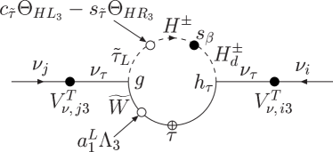
Refer to caption Refer to caption
Figure 9: H±superscript𝐻plus-or-minusH^{\pm} contribution to ΔB0H±τ~1Δsuperscriptsubscript𝐵0superscript𝐻plus-or-minussubscript~𝜏1\Delta B_{0}^{H^{\pm}\tilde{\tau}_{1}}
Refer to caption Refer to caption
Figure 10: τ~1subscript~𝜏1\tilde{\tau}_{1} contributions to ΔB0H±τ~1Δsuperscriptsubscript𝐵0superscript𝐻plus-or-minussubscript~𝜏1\Delta B_{0}^{H^{\pm}\tilde{\tau}_{1}} and ΔB0G±τ~1τ~2Δsuperscriptsubscript𝐵0superscript𝐺plus-or-minussubscript~𝜏1subscript~𝜏2\Delta B_{0}^{G^{\pm}\tilde{\tau}_{1}\tilde{\tau}_{2}}

There is another set of four graphs corresponding to τ~2subscript~𝜏2{\tilde{\tau}_{2}} that are obtained from those in Fig. 10 by replacing τ~1τ~2subscript~𝜏1subscript~𝜏2\tilde{\tau}_{1}\rightarrow\tilde{\tau}_{2}, sτ~cτ~subscript𝑠~𝜏subscript𝑐~𝜏s_{\tilde{\tau}}\rightarrow c_{\tilde{\tau}} and cτ~sτ~subscript𝑐~𝜏subscript𝑠~𝜏c_{\tilde{\tau}}\rightarrow-s_{\tilde{\tau}}. These three groups of four graphs, when combined, form a set which is ultraviolet finite and account for the terms in Eq. (33) proportional to ΔB0H+τ~1Δsuperscriptsubscript𝐵0superscript𝐻subscript~𝜏1\Delta B_{0}^{H^{+}\tilde{\tau}_{1}} and ΔB0H+τ~2Δsuperscriptsubscript𝐵0superscript𝐻subscript~𝜏2\Delta B_{0}^{H^{+}\tilde{\tau}_{2}}.

C.3 ΔB0H±L1Δsuperscriptsubscript𝐵0superscript𝐻plus-or-minussubscript𝐿1\Delta B_{0}^{H^{\pm}L_{1}} and ΔB0H±L2Δsuperscriptsubscript𝐵0superscript𝐻plus-or-minussubscript𝐿2\Delta B_{0}^{H^{\pm}L_{2}}

Refer to caption Refer to caption
Figure 11: a) H±superscript𝐻plus-or-minusH^{\pm} contribution to ΔB0H±L1Δsuperscriptsubscript𝐵0superscript𝐻plus-or-minussubscript𝐿1\Delta B_{0}^{H^{\pm}L_{1}}; b) e~Lsubscript~𝑒𝐿\tilde{e}_{L} contribution to ΔB0H±L1Δsuperscriptsubscript𝐵0superscript𝐻plus-or-minussubscript𝐿1\Delta B_{0}^{H^{\pm}L_{1}} and ΔB0G±L1Δsuperscriptsubscript𝐵0superscript𝐺plus-or-minussubscript𝐿1\Delta B_{0}^{G^{\pm}L_{1}}

We now turn our attention to the terms proportional to ΔB0H±L1Δsuperscriptsubscript𝐵0superscript𝐻plus-or-minussubscript𝐿1\Delta B_{0}^{H^{\pm}L_{1}} and B0H±L2superscriptsubscript𝐵0superscript𝐻plus-or-minussubscript𝐿2B_{0}^{H^{\pm}L_{2}} which are related to the mixing between charged Higgs with selectrons and smuons. The terms proportional to ΔB0H±L1Δsuperscriptsubscript𝐵0superscript𝐻plus-or-minussubscript𝐿1\Delta B_{0}^{H^{\pm}L_{1}} come from the diagrams of Fig. 11. The terms proportional to ΔB0H±L2Δsuperscriptsubscript𝐵0superscript𝐻plus-or-minussubscript𝐿2\Delta B_{0}^{H^{\pm}L_{2}} are easily obtained from these by replacing the corresponding slepton lines and couplings. Notice that in Fig. 11 b) there is a contribution proportional to v1/vsubscript𝑣1𝑣v_{1}/v that does not belong to this term. We will show below that it will contribute to the ΔB0G±L1Δsuperscriptsubscript𝐵0superscript𝐺plus-or-minussubscript𝐿1\Delta B_{0}^{G^{\pm}L_{1}} term.

C.4 ΔB0G±L1Δsuperscriptsubscript𝐵0superscript𝐺plus-or-minussubscript𝐿1\Delta B_{0}^{G^{\pm}L_{1}} and ΔB0G±L2Δsuperscriptsubscript𝐵0superscript𝐺plus-or-minussubscript𝐿2\Delta B_{0}^{G^{\pm}L_{2}}

Refer to caption
Figure 12: G±superscript𝐺plus-or-minusG^{\pm} contribution to ΔB0G±L1Δsuperscriptsubscript𝐵0superscript𝐺plus-or-minussubscript𝐿1\Delta B_{0}^{G^{\pm}L_{1}}

The graphs contributing to the ΔB0G±L1Δsuperscriptsubscript𝐵0superscript𝐺plus-or-minussubscript𝐿1\Delta B_{0}^{G^{\pm}L_{1}} and ΔB0G±L2Δsuperscriptsubscript𝐵0superscript𝐺plus-or-minussubscript𝐿2\Delta B_{0}^{G^{\pm}L_{2}} terms are related to those of Fig. 11. They are given by Fig. 12 and by the term proportional to v1/vsubscript𝑣1𝑣v_{1}/v in Fig. 11 b), for the case of the selectron. The terms proportional to ΔB0G±L2Δsuperscriptsubscript𝐵0superscript𝐺plus-or-minussubscript𝐿2\Delta B_{0}^{G^{\pm}L_{2}} are easily obtained from these by replacing the corresponding slepton lines and couplings.

C.5 ΔB0G±τ~1τ~2Δsuperscriptsubscript𝐵0superscript𝐺plus-or-minussubscript~𝜏1subscript~𝜏2\Delta B_{0}^{G^{\pm}\tilde{\tau}_{1}\tilde{\tau}_{2}}

We now consider a more complicated term, the one proportional to ΔB0G±τ~1τ~2Δsuperscriptsubscript𝐵0superscript𝐺plus-or-minussubscript~𝜏1subscript~𝜏2\Delta B_{0}^{G^{\pm}\tilde{\tau}_{1}\tilde{\tau}_{2}}. This term gives a finite ultraviolet contribution and comes from the diagrams of Fig. 13, together with the parts of the diagrams of Fig. 10 that are proportional to v3/vsubscript𝑣3𝑣v_{3}/v. Corresponding to the diagrams in Fig. 13 proportional to v3/vsubscript𝑣3𝑣v_{3}/v, there is another set with τ~1subscript~𝜏1\tilde{\tau}_{1} and τ~2subscript~𝜏2\tilde{\tau}_{2} interchanged in the usual way.

Refer to caption Refer to caption
Figure 13: G±superscript𝐺plus-or-minusG^{\pm} contribution to ΔB0G±τ~1τ~2Δsuperscriptsubscript𝐵0superscript𝐺plus-or-minussubscript~𝜏1subscript~𝜏2\Delta B_{0}^{G^{\pm}\tilde{\tau}_{1}\tilde{\tau}_{2}}

C.6 ΔB0G±H±τ~1τ~2Δsuperscriptsubscript𝐵0superscript𝐺plus-or-minussuperscript𝐻plus-or-minussubscript~𝜏1subscript~𝜏2\Delta B_{0}^{G^{\pm}H^{\pm}\tilde{\tau}_{1}\tilde{\tau}_{2}}

Let us consider finally the last term in Eq. (33), the one proportional to ΔB0G±H±τ~1τ~2Δsuperscriptsubscript𝐵0superscript𝐺plus-or-minussuperscript𝐻plus-or-minussubscript~𝜏1subscript~𝜏2\Delta B_{0}^{G^{\pm}H^{\pm}\tilde{\tau}_{1}\tilde{\tau}_{2}}. This term gives an ultraviolet finite contribution and comes from four diagrams. The first two are those represented in Fig. 14 corresponding to a H±superscript𝐻plus-or-minusH^{\pm} and τ~1subscript~𝜏1\tilde{\tau}_{1} propagating in the loop. The other two are obtained from these with the replacements,

H±G±superscript𝐻plus-or-minussuperscript𝐺plus-or-minusH^{\pm}\rightarrow\ G^{\pm} , sβcβsubscript𝑠𝛽subscript𝑐𝛽\ s_{\beta}\rightarrow c_{\beta}
τ~1τ~2subscript~𝜏1subscript~𝜏2\tilde{\tau}_{1}\rightarrow\ \tilde{\tau}_{2} , sτ~cτ~subscript𝑠~𝜏subscript𝑐~𝜏\ s_{\tilde{\tau}}\rightarrow c_{\tilde{\tau}}
(73)
Refer to caption Refer to caption
Figure 14: H±superscript𝐻plus-or-minusH^{\pm} and τ~1subscript~𝜏1\tilde{\tau}_{1} contributions to ΔB0G±H±τ~1τ~2Δsuperscriptsubscript𝐵0superscript𝐺plus-or-minussuperscript𝐻plus-or-minussubscript~𝜏1subscript~𝜏2\Delta B_{0}^{G^{\pm}H^{\pm}\tilde{\tau}_{1}\tilde{\tau}_{2}}

References

  • [1] Q. R. Ahmad et al. [SNO Collaboration], Phys. Rev. Lett. 89, 011301 (2002) [arXiv:nucl-ex/0204008].
  • [2] M. Maltoni, T. Schwetz, M. A. Tortola and J. W. Valle, arXiv:hep-ph/0207227, to be published in Phys. Rev. D. This contains a full set of references on pre-KamLAND analyses of solar neutrino data. For references to relevant experimental papers see Pakvasa:2003zv
  • [3] K. Eguchi et al, [KamLAND Collaboration], arXiv:hep-ex/0212021.
  • [4] For a recent review see S. Pakvasa and J. W. Valle, arXiv:hep-ph/0301061.
  • [5] M. Maltoni, T. Schwetz and J. W. Valle, arXiv:hep-ph/0212129, for a full set of references on post-KamLAND analyses of solar neutrino data see  Pakvasa:2003zv .
  • [6] M. C. Gonzalez-Garcia, P. C. de Holanda, C. Pena-Garay and J. W. Valle, Nucl. Phys. B 573, 3 (2000) [arXiv:hep-ph/9906469].
  • [7] Y. Fukuda et al. [Super-Kamiokande Collaboration], Phys. Rev. Lett. 81, 1562 (1998) [arXiv:hep-ex/9807003].
  • [8] M Gell-Mann, P Ramond, R. Slansky, in Supergravity, ed. P. van Niewenhuizen and D. Freedman (North Holland, 1979); T. Yanagida, in KEK lectures, ed. O. Sawada and A. Sugamoto (KEK, 1979)
  • [9] R. N. Mohapatra and G. Senjanovic, Phys. Rev. D 23, 165 (1981).
  • [10] J. Schechter and J. W. Valle, Phys. Rev. D 25, 774 (1982).
  • [11] G. G. Ross and J. W. Valle, Phys. Lett. B 151 (1985) 375. L. J. Hall and M. Suzuki, Nucl. Phys. B 231, 419 (1984). J. R. Ellis et al, Phys. Lett. B 150 (1985) 142. C. S. Aulakh and R. N. Mohapatra, Phys. Lett. B 119 (1982) 13 A. Santamaria and J. W. Valle, Phys. Lett. B 195, 423 (1987). Phys. Rev. Lett.  60, 397 (1988). Phys. Rev. D 39, 1780 (1989).
  • [12] M. A. Diaz, J. C. Romao and J. W. Valle, Nucl. Phys. B 524, 23 (1998) [arXiv:hep-ph/9706315]. For a review see J. W. Valle, arXiv:hep-ph/9808292.
  • [13] A. Bartl, W. Porod, D. Restrepo, J. Romao and J. W. Valle, Nucl. Phys. B 600 (2001) 39 [arXiv:hep-ph/0007157].
  • [14] W. Porod, M. Hirsch, J. Romao and J. W. Valle, Phys. Rev. D 63, 115004 (2001) [arXiv:hep-ph/0011248].
  • [15] B. Mukhopadhyaya, S. Roy and F. Vissani, Phys. Lett. B 443, 191 (1998) [arXiv:hep-ph/9808265].
  • [16] S. Y. Choi, E. J. Chun, S. K. Kang and J. S. Lee, Phys. Rev. D 60, 075002 (1999) [arXiv:hep-ph/9903465].
  • [17] M. Hirsch, W. Porod, J. C. Romao and J. W. Valle, Phys. Rev. D 66 (2002) 095006 [arXiv:hep-ph/0207334].
  • [18] D. Restrepo, W. Porod and J. W. Valle, Phys. Rev. D 64, 055011 (2001) [arXiv:hep-ph/0104040].
  • [19] B. Allanach et al., arXiv:hep-ph/9906224.
  • [20] F. de Campos et al, Nucl. Phys. B 451, 3 (1995) [arXiv:hep-ph/9502237]. Y. Grossman and H. E. Haber, Phys. Rev. D 63, 075011 (2001) [arXiv:hep-ph/0005276].
  • [21] T. Banks, Y. Grossman, E. Nardi and Y. Nir, Phys. Rev. D 52, 5319 (1995) [arXiv:hep-ph/9505248].
  • [22] B. de Carlos and P. L. White, Phys. Rev. D 54, 3427 (1996) [arXiv:hep-ph/9602381].
  • [23] A. G. Akeroyd et al, Nucl. Phys. B 529, 3 (1998) [arXiv:hep-ph/9707395].
  • [24] F. de Campos, O. J. P. Éboli, M. A. García–Jareño and J. W. F. Valle, Nucl. Phys. B 546, 33 (1999); R. Kitano and K. Oda, Phys. Rev. D 61, 113001 (2000); D. E. Kaplan and A. E. Nelson, JHEP 0001, 033 (2000); C.–H. Chang and T.–F. Feng, Eur. Phys. J. C12, 137 (2000); M. Frank, Phys. Rev. D 62, 015006 (2000); F. Takayama and M. Yamaguchi, Phys. Lett. B 476, 116 (2000); K. Choi, E. J. Chun and K. Hwang, Phys. Lett. B 488, 145 (2000); M.A. Diaz, R.A. Lineros, M.A. Rivera, hep-ph/0210182; F. De Campos, M.A. Diaz, O.J.P. Eboli, M.B. Magro, P.G. Mercadante, Nucl. Phys. B 623, 47 (2002).
  • [25] A. S. Joshipura and M. Nowakowski, Phys. Rev. D 51, 2421 (1995); G. Bhattacharyya, D. Choudhury and K. Sridhar, Phys. Lett. B 349, 118 (1995); A. Yu. Smirnov and F. Vissani, Nucl. Phys. B 460, 37 (1996); J. C. Romão, F. de Campos, M. A. García–Jareño, M. B. Magro and J. W. F. Valle, Nucl. Phys. B 482, 3 (1996); R. Hempfling, Nucl. Phys. B 478, 3 (1996);
  • [26] M. A. Díaz, J. Ferrandis, J. C. Romão and J. W. F. Valle, Phys. Lett. B 453, 263 (1999); A. G. Akeroyd, M. A. Díaz and J. W. F. Valle, Phys. Lett. B 441, 224 (1998); M. A. Díaz, E. Torrente–Lujan and J. W. F. Valle, Nucl. Phys. B 551, 78 (1999); M. A. Díaz, J. Ferrandis, J. C. Romão and J. W. F. Valle, Nucl. Phys. B 590, 3 (2000); M. A. Díaz, D. A. Restrepo and J. W. F. Valle, Nucl. Phys. B 583, 182 (2000); M. A. Díaz, J. Ferrandis and J. W. F. Valle, Nucl. Phys. B 573, 75 (2000).
  • [27] S. Roy, B. Mukhopadhyaya, Phys. Rev. D 55, 7020 (1997); K. Cheung, O.C.W. Kong, Phys. Rev. D 64, 095007 (2001); T.F. Feng, X.Q. Li, Phys. Rev. D 63, 073006 (2001); E.J. Chun, S.K. Kang, Phys. Rev. D 61, 075012 (2000); J. Ferrandis, Phys. Rev. D 60, 095012 (1999); A.G. Akeroyd, C. Liu, J. Song, Phys. Rev. D 65, 015008 (2002); D. Suematsu, Phys. Lett. B 506, 131 (2001).
  • [28] M. Hirsch, M. A. Diaz, W. Porod, J. C. Romao and J. W. Valle, Phys. Rev. D 62, 113008 (2000) [Erratum-ibid. D 65, 119901 (2002)] [arXiv:hep-ph/0004115]; J. C. Romao, M. A. Diaz, M. Hirsch, W. Porod and J. W. Valle, Phys. Rev. D 61, 071703 (2000) [arXiv:hep-ph/9907499].
  • [29] E. J. Chun, D. W. Jung and J. D. Park, arXiv:hep-ph/0211310. F. Borzumati and J. S. Lee, Phys. Rev. D 66 (2002) 115012 [arXiv:hep-ph/0207184]. E. J. Chun and J. S. Lee, Phys. Rev. D 60, 075006 (1999) [arXiv:hep-ph/9811201]. A. Abada, S. Davidson and M. Losada, Phys. Rev. D 65 (2002) 075010 [arXiv:hep-ph/0111332].
  • [30] A. Masiero and J. W. Valle, Phys. Lett. B 251, 273 (1990).
  • [31] J. C. Romao, C. A. Santos and J. W. Valle, Phys. Lett. B 288, 311 (1992).
  • [32] J. C. Romao and J. W. Valle, Nucl. Phys. B 381 (1992) 87; J. C. Romao, F. de Campos and J. W. Valle, Phys. Lett. B 292 (1992) 329 [arXiv:hep-ph/9207269]; M. Shiraishi, I. Umemura and K. Yamamoto, Phys. Lett. B 313 (1993) 89. For bounds on spontaneous R-parity violation see P. Abreu et al. [DELPHI Collaboration], Phys. Lett. B 502 (2001) 24 [arXiv:hep-ex/0102045] and D. Magalhaes Moraes, CERN-THESIS-2002-021
  • [33] J. M. Mira, E. Nardi, D. A. Restrepo and J. W. Valle, Phys. Lett. B 492 (2000) 81 [arXiv:hep-ph/0007266].
  • [34] G. F. Giudice and A. Masiero, Phys. Lett. B 206, 480 (1988).
  • [35] H. P. Nilles and N. Polonsky, Nucl. Phys. B 484, 33 (1997) [arXiv:hep-ph/9606388].
  • [36] M. Hirsch and J. W. Valle, Nucl. Phys. B 557, 60 (1999) [arXiv:hep-ph/9812463].
  • [37] M. Nowakowski and A. Pilaftsis, Nucl. Phys. B 461, 19 (1996).
  • [38] G. Passarino and M. J. Veltman, Nucl. Phys. B 160 (1979) 151
  • [39] Numerical algorithms for Passarino-Veltman functions have been published in: G. J. van Oldenborgh and J. A. Vermaseren, Z. Phys. C 46 (1990) 425; T. Hahn, M. Perez-Victoria, Comput.Phys.Commun. 118 (1999) 153, see http://www.feynarts.de/looptools/;