OITS-725

Higgs pair production in association with a vector boson at $e^{+}e^{-}$ colliders in theories of higher dimensional gravity
N. G. Deshpande, Dilip Kumar Ghosh

Institute of Theoretical Science
5203 University of Oregon
Eugene OR 97403-5203

The models of large extra compact dimensions, as suggested by Arkani-Hamed, Dimopoulos and Dvali, predict exciting phenomenological consequences with gravitational interactions becoming strong at the TeV scale. Such theories can be tested at the existing and future colliders. In this paper, we study the contribution of virtual Kaluza-Klein excitations (both spin-0 and 2) in the process $e^{+}e^{-}\to HHZ$ and $e^{+}e^{-}\to HH\gamma$ at future linear collider (NLC). We find that the virtual exchange KK gravitons can modify the cross-section $\sigma(e^{+}e^{-}\to HHZ)$ significantly from its Standard Model value and will allow the effective string scale to be probed up to 6.6 TeV. The second process is absent at the tree level in the standard model, and can therefore be used to put limits on the effective string scale of 7.4 TeV.

1 Introduction

The concept of large extra dimensions and TeV scale gravity introduced by Arkhani-Hamed, Dimopoulos and Dvali, better known as ADD model [1] has attracted a lot of attention. In this scenario, the total space-time has $D=4+n$ dimensions, where gravity lives in $n$ additional large spatial dimensions of size $R$. The standard model particles are confined to the usual $3+1$-dimension.

The effective $4D$ Planck scale, $M_{Pl}\sim 2.4\times 10^{18}$ GeV , is related to the fundamental Planck scale $M_{S}$ in $(4+n)$ dimension by

$$M^{2}_{Pl}\sim R^{n}M^{n+2}_{S}$$ (1)

Thus, for the large extra-dimensions, it is possible to have a fundamental scale $M_{S}$ as low as a TeV [1], solving the gauge hierarchy problem of the standard model. With $M_{S}\sim$ TeV, for $n=1$ the value of $R$ ($\sim 10^{11}$ millimeter ) is ruled out by gravitational experiments. On the other hand, $n\geq 2$, we get $R\leq$ mm, a range that is still allowed by gravitational experiments.

Each graviton couples to the standard model matter and gauge particles through energy-momentum tensor and its trace, with the strength suppressed by powers of the $4$-dimensional Planck scale, $M_{Pl}$. However, from the 4-dimensional point of view, the massless gravitons propagating in the $(4+n)$-dimensional bulk are seen as massive towers of Kaluza-Klein (KK) modes of excitations with spin-0, spin-1 (which decouples ) and spin-2. The mass spectrum of these KK modes can be treated as a continuum, since their mass splitting $\sim 1/R$ is about $10^{-4}$ eV for $n=2$ and for $n=6$ it is of the order of a MeV. After summing over these KK modes one gets enhancement of KK graviton coupling to standard model matter and gauge particles to powers of $(\sqrt{s}/M_{S})$ [1], where $\sqrt{s}$ is the available energy for the process. The Feynman rules for this theory have been developed considering a linearized theory of gravity in the bulk in Ref.  [2, 3]. These new interactions can give rise to several interesting phenomenological consequences testable at present and future colliders [4]. The effect of these new interactions can be observed either through production of real KK modes, or through the exchange of virtual KK modes in various processes [4, 5, 6].

In this paper we will consider the process $e^{+}e^{-}\to HHZ$ and $e^{+}e^{-}\to HH\gamma$ to study the effect of low-scale gravity at proposed linear colliders with center of mass energy 500 GeV and beyond. However, one should keep in mind that these processes will not serve as the dominant discovery channel for KK gravitons, since there are more direct processes for its discovery [4]. Once the discovery of KK gravitons is established, then the next phase will be to look for their effect on some more complicated processes, like the ones discussed here, to re-confirm their discovery.

In the standard model, $HHZ$ production has been studied in the context of the determination of the Higgs self couplings  [8]. The other channel, $HH\gamma$, is a unique process mediated by virtual gravitons. This process is absent at the tree level in the standard model, therefore, the observation of such a process can lead to a possible indication of low scale gravity. Through out this paper we assume that the Higgs boson will already have been discovered and its mass determined.

The rest of the paper is organized as follows: In Section 2, we study the production of $HHZ$ and discuss the effect of KK gravitons. In Section 3, we will discuss how virtual exchange of gravitons give rise to $HH\gamma$ final state and discuss the consequences. Section 4 is reserved for the overall discussions and conclusions. In Appendix, we present the graviton exchange amplitudes for $e^{+}e^{-}\to HHZ$ process.

2 $e^{+}e^{-}\to HHZ$

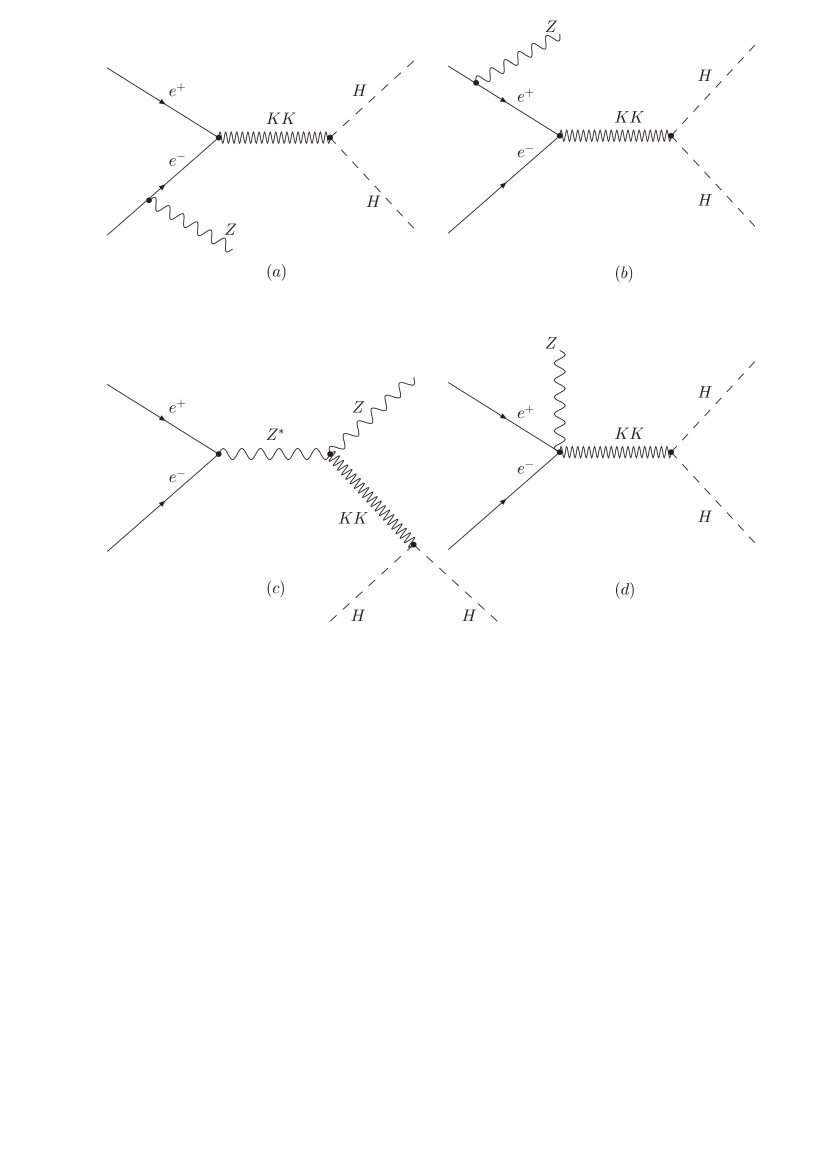
Figure 1: Feynman diagrams of virtual gravitons ( both spin-0 and spin-2) contribution to the process $e^{+}e^{-}\to HHZ$.

In this section we study the additional contribution of virtual exchange of spin 2 and 0 graviton modes in models of large extra dimensions to the Higgs pair production in association with $Z$. In the standard model, the process $e^{+}e^{-}\to HHZ$ has been studied as a means of determining $HHH$ couplings. The standard model amplitudes and polarized cross-sections are given in the Ref.[8]. In our analysis, we shall use unpolarized beams. Additional diagrams arising from the exchange of both spin-2 and spin-0 KK gravitons are shown in Figure 1, where $KK$ stands for both the spin-2 and spin-0 modes. The amplitudes using the Feynman rules given in Ref.[3] are presented in the Appendix.

After adding coherently these new amplitudes to the standard model ones, we get the total amplitude. The new amplitude now depends on Higgs boson mass($M_{H}$), center-of-mass energy($\sqrt{s}$), fundamental Planck scale ($M_{S}$), and finally on the number of extra dimensions $(n$). Through out our analysis we have fixed the standard model Higgs boson mass at a representative value $M_{H}=120$ GeV. For center of mass energy, we consider three possible values of $\sqrt{s}=0.5$ TeV, $1$ TeV and $3$ TeV at which the future $e^{+}e^{-}$ colliders are expected to operate [5, 6, 7].

In Figure 2, we represent the total cross-section for $M_{H}=120$ GeV and $n=3$ as a function of machine energy for three different values of $M_{S}=3.5,4.5$ and $5.5$ TeV. The dashed line represents the standard model prediction and this exhibits the expected fall-off behavior with energy. For large values of $M_{S}$, this behavior is preserved, since the graviton contribution then becomes small. However, when $M_{S}$ is smaller, the cross-section show a marked increase with energy, showing the well-known feature of gravitational interaction. It is obvious from this Figure, that at energies around 3 TeV, the graviton contribution is enormous, if $M_{S}$ is small ( 3.5 TeV); however, a discernible difference exists even when $M_{S}=5.5$ TeV. Thus we can expect larger effects, or in other words stronger bounds on $M_{S}$ as the machine energy increases.

In Figure 3, we represent the total cross-section as a function of $M_{S}$ for different values of extra dimensions $n=3,4,5,6$ for two value of machine energies, $\sqrt{s}=500$ GeV and 1 TeV. For comparison the standard model cross-sections are given by the dashed lines, which are independent of $M_{S}$. From this Figure, we can see that for a given machine energy and $M_{S}$, the graviton contribution decreases with the increase in extra-dimension $(n)$. For a given $n$, the graviton contribution asymptotically tends to the standard model value with increase of $M_{S}$ as it should.

In Figure 4, we represent the angular distribution of the Higgs boson. The standard model distribution (dashed line) shows typical $\sin^{2}\theta$ behavior, whereas, the ADD contribution (solid line), which has in addition spin-2 and spin-0 exchange, can be distinguished from the standard model very easily. From this distribution, it is evident that larger deviation from the standard model is expected in the forward and backward regions of the detector, with $0.5<\mid\cos\theta\mid<0.8$. We assume that the efficiency of the detectors in that region will be good enough to observe such events. In the central region ( $\mid\cos\theta\mid<0.2$ ) of the detector, the standard model cross-section shows a peak over the ADD contribution.

In Figure 5, we represent the fractional deviation $R=\frac{\mid\sigma(M_{S})-\sigma_{SM}\mid}{\sigma_{SM}}$ as a function of $M_{S}$ for two values of center of energies, 500 GeV (dashed line), and 1 TeV ( solid line ), where, $\sigma(M_{S})$ is obtained from coherent sum of ADD and standard model amplitudes. The different choices of extra dimensions $(n)$ are shown along each curve. It is very clear from this Figure, that higher the machine energy, larger is the deviation from the standard model. We consider that more than $10\%$ deviation $(R=0.1)$ from the standard model prediction with an integrated luminosity ${\cal L}$ of $2{\rm ab}^{-1}$ will be able to provide reasonable evidence of low-scale gravity. This argument is based on the result obtained in Ref.[9]. In this paper, the authors have studied the standard model $ZHH$ production at future $e^{+}e^{-}$ linear collider. They have shown that at $\sqrt{s}=500$ GeV, the $e^{+}e^{-}\to ZHH$ cross-section can be determined with a $10\%$ relative error assuming an integrated luminosity of $2{\rm ab}^{-1}$. In our analysis we use this error ($10\%$) on the cross-section measurement to determine $5\sigma$ discovery limit on $M_{S}$ with the same integrated luminosity.

For higher center-of-mass energies$(\sqrt{s}=1$ TeV and 3 TeV), we also assume for simplicity the same relative error in the $ZHH$ cross-section measurement with the same integrated luminosity. We think as a first exercise of this kind, the assumption considered here is sufficient. Before we display our limits on the scale $M_{S}$, we would also like to stress that the limits on the string scale $M_{S}$ obtained here are merely indicative. These limits may change when one considers detector simulations with full estimations of signal and backgrounds. As we have already mentioned, this process should not be considered as the main channel to probe the low scale quantum gravity. Since, by the time the next future $e^{+}e^{-}$ collider starts operating and reaches such a high integrated luminosity, the low scale quantum gravity model would have been discovered if true.

In the Table 1, we display the $5\sigma$ discovery limits on $M_{S}$ as a function of $e^{+}e^{-}$ center of mass energy $(\sqrt{s})$, number of extra-dimensions $(n)$ and integrated luminosity. From this Table, we can appreciate the following features:

• The $5\sigma$ limit on $M_{S}$ is weekly dependent on number of extra dimensions $(n)$.

• The $5\sigma$ limit on $M_{S}$ obtained for 500 GeV machine is not very promising. In this case the strongest limit is less than 1 TeV for $n=3$.

• The situation become better once we go to a higher center of mass energy. The strongest limit on $M_{S}$ is 6.6 TeV obtained for $n=3$ and at $\sqrt{s}=3$ TeV.

$\sqrt{s}$	$M_{S}$ in GeV
TeV	$n=3$	4	5	6
0.5	921	769	697	653
1.0	1998	1811	1685	1593
3.0	6598	6036	5634	5332

Table 1: $5\sigma$ limit on $M_{S}$ assuming an integrated luminosity of $2~{}{\rm ab}^{-1}$ for different center of mass energies ($\sqrt{s}$). $n$ is the number of extra dimensions.

3 $e^{+}e^{-}\to HH\gamma$

For the completeness of our study, in this section we discuss the production of $HH\gamma$ at $e^{+}e^{-}$ collider through the virtual exchange of spin-2 and spin-0 KK gravitons. The scalar pair production at $e^{+}e^{-}$ collider in the models of large extra-dimensions has been studied [10]. The Feynman diagrams for $e^{+}e^{-}\to HH\gamma$ are similar to Figure 1, with $Z$ replaced by $\gamma$. In the case of exchange of spin-2 gravitons all the four diagrams $(a-d)$ contribute, while for spin-0 KK mode exchange, only diagrams $(a)$,$(b)$ and $(d)$ contribute. These three diagrams form a gauge invariant set, while the diagram $(c)$ vanishes due to Dirac equation and gauge invariance. In this process, unlike Higgs boson pair production, spin-0 mode of KK graviton also contribute. The photon will serve as an additional trigger. We impose the following identification criteria for the photon  [11]:

$$E_{\gamma} > 10~{}~{}{\rm GeV}$$ (2)

$$\mid\cos\theta_{\gamma}\mid < 0.98$$ (3)

where, $\theta_{\gamma}$ defines the photon angle with the $e^{-}$ beam direction. This angular cut on the photon removes the collinear divergence. These ‘acceptance’ cuts are more-or-less the basic ones. Though further selection cuts will become appropriate when a more detailed analysis is done, it suffices for our analysis, which is a preliminary study.

Unlike the previous case, here the whole contribution comes from the exchange of virtual gravitons. As before, we fix the Higgs boson mass at the value used in the last section as also the machine energies.

In Figure 6, we represent the total cross-section for $M_{H}=120$ GeV and $n=3$ as a function of machine energy for three different values of $M_{S}=3.5,4.5$ and $5.5$ TeV. For a given $M_{S}$, the cross-section shows a marked increase with energy, depicting the well-known feature of gravitational interaction.

It is obvious from this Figure, that at energies around 3 TeV, the graviton contribution is enormous, if the $M_{S}$ is small ( 3.5 TeV); however, a discernible difference exists even when $M_{S}=5.5$ TeV. Thus we can expect larger effects, or in other words stronger bounds on $M_{S}$ as the machine energy increases. In Figure 7, we represent the angular distribution of the Higgs boson. This particular shape of the distribution is specific to virtual exchange of gravitons in the process.

In Figure 8, we represent the total production cross-section as a function of $M_{S}$ for different values of extra-dimensions $n=3,4,5,6$ for three values of center-of-mass energies, $\sqrt{s}=500$ GeV (dotted lines), 1 TeV (dashed lines ) and 3 TeV ( solid lines). For a given $\sqrt{s}$ and $M_{S}$, the graviton contribution decreases very slowly with increase of extra-dimension $n$.

The main possible source of background to this process is $e^{+}e^{-}\to ZH\gamma$ with $Z$ decays to $b\bar{b}$ looking like a Higgs decay. Using the CompHEP [12] we have computed $\sigma^{B}_{eff}(=\sigma(e^{+}e^{-}\to ZH\gamma)\times Br(Z\to b{\bar{b}}))\times Br(H\to b{\bar{b}}))$ for $e^{+}e^{-}\to ZH\gamma$ process for three values of $\sqrt{s}=0.5$ TeV, 1 TeV and 3 TeV to get a feeling for this background. The numbers are 0.50 fb, 0.15 fb and 0.023 fb for $\sqrt{s}=0.5$ TeV, 1 TeV and 3 TeV respectively. There are two ways one can eliminate this background. Firstly, if the Higgs mass is heavier than $M_{Z}$ (which is in fact true from LEP II data) [13], the invariant mass distribution of particles produced from Higgs decay will be able to reduce the background. Secondly, it should also be possible to reduce the background further by studying the angular distribution associated with these processes. The loop-induced standard model or MSSM Higgs pair production cross-section for light Higgs mass is of the order $0.1-0.2$ fb at $\sqrt{s}=500$ GeV [14]. This cross-section will be suppressed by order $\alpha_{em}$, if an additional photon is produced. When folded with $H\to b\bar{b}$ branching ratio, the cross-section becomes $O(10^{-4})$ fb. This cross-section will be further suppressed by the 3 body phase-space.

To estimate the possible $5\sigma$ discovery limit on the scale $M_{S}$ with an integrated luminosity of $2{\rm ab}^{-1}$, we only consider the $ZH\gamma$ as the main source of standard model background. We multiply the standard model cross-section by the luminosity to get the predicted number of events. We then estimate the errors assuming that the statistical errors are Gaussian and that there are no systematic errors. This certainly makes our estimates of the discovery limits over-optimistic ( especially for for $\sqrt{s}=3$ TeV, where number of standard model events are small ). In any case, before more detailed studies of the standard model backgrounds and the detector design, any estimate of errors must be considered a crude estimate. In Table 2 we display such discovery limits on $M_{S}$ for different machine energies and extra-dimensions. As expected the strongest limit appears for $\sqrt{s}=3$ TeV and for $n=3$.

$\sqrt{s}$	$M_{S}$ in GeV
TeV	$n=3$	4	5	6
0.5	1557	1175	993	883
1.0	2847	2154	1834	1637
3.0	7383	5673	4866	4383

Table 2: $5\sigma$ discovery limit on $M_{S}$ assuming an integrated luminosity of $2~{}{\rm ab}^{-1}$ for different center-of-mass energies ($\sqrt{s}$). $n$ is the number of extra dimensions.

4 Conclusions

In this paper we have studied the implications of KK graviton contribution to the process $e^{+}e^{-}\to HHZ$, which has been studied in the standard model. The spin-2 and spin-0 mode of KK gravitons contribute to this process substantially. However, the existence of low-energy quantum gravity may be discovered through more direct channels as studied by several groups. Nevertheless, this process will be an independent confirmation for such a discovery. The $5\sigma$ discovery limits on the string scale $M_{S}$ is obtained assuming an integrated luminosity of $2~{}{\rm ab}^{-1}$. We have derived this limit considering $10\%$ error on the $HHZ$ cross-section measurement at $\sqrt{s}=500$ GeV at ${\cal L}=2~{}{\rm ab}^{-1}$. In reality for higher center-of-mass energies, the above error may change. However, in our analysis we have assumed it to be remain the same. The bounds obtained here are only suggestive and may change when one take into account proper detector simulation, inclusing $H$ and $Z$ decays and imposing selection cuts on the final state particles and the full background calculation.

Another interesting behavior is shown by the Higgs angular distributions. In the standard model, the shape behaves like $\sim\sin^{2}\theta$, whereas it is completely different in the presence of KK gravitons. Furthermore, we have shown that in the forward and backward regions of the beam pipe, one would expect larger deviation from the standard model prediction. Hence, careful study of Higgs angular distribution may provide evidence of new physics beyond the standard model.

To complete our analysis we have also studied the $e^{+}e^{-}\to HH\gamma$ process in this model which is absent at the tree level in the standard model. We have discussed how this mode can be distinguished from the possible backgrounds. We have obtained the $5\sigma$ discovery limit on $M_{S}$ assuming an integrated luminosity of $2~{}{\rm ab}^{-1}$.

5 Appendix

Here we will write down the graviton contribution ( both spin 2 and $0$ ) amplitudes for the process :$e^{+}e^{-}\to HHZ$. In our analysis we have chosen $\xi=1$, the so called de Donder gauge. The Feynman rules used to obtain these matrix elements have been taken from Ref.[3]. The relation between the fundamental scale $M_{S}$ and the size $R$ of the $n$ extra dimensions is given by [3]

$$\kappa^{2}R^{n}=16\pi(4\pi)^{n/2}\Gamma(n/2)M_{S}^{-(n+2)}$$ (4)

where, $\kappa=\sqrt{16\pi G_{N}}$. $G_{N}$ is the four dimensional Newton constant. The amplitudes $a-d$ and $e-h$ correspond to the exchange of a virtual graviton of spin $2$ and $0$ respectively.

$${\cal M}_{a} = -\frac{\pi g}{2C_{W}}{\cal G}\frac{P^{\mu\nu\alpha\beta}}{(k_{1}-p_{1})^{2}}{\cal X}_{\alpha\beta}\big{[}{\bar{v}(k_{2})}C_{\mu\nu}({k_{1}/\;\>}-{p_{1}/\;\>})\gamma^{\rho}(g_{v}+g_{a}\gamma_{5})u(k_{1})\big{]}\epsilon^{*}_{\rho}(p_{1})$$ (5)

$${\cal M}_{b} = \frac{\pi g}{2C_{W}}{\cal G}\frac{P^{\mu\nu\alpha\beta}}{(k_{2}-p_{1})^{2}}{\cal X}_{\alpha\beta}\big{[}{\bar{v}(k_{2})}\gamma^{\rho}(g_{v}+g_{a}\gamma_{5})({k_{2}/\;\>}-{p_{1}/\;\>})C^{\prime}_{\mu\nu}u(k_{1})\big{]}\epsilon^{*}_{\rho}(p_{1})$$ (6)

$${\cal M}_{c} = \frac{2\pi g}{C_{W}}{\cal G}\frac{P^{\rho\sigma\alpha\beta}}{(s-M^{2}_{Z})}{\cal F}_{\rho\sigma\nu\lambda}(g^{\mu\nu}-\frac{q^{\mu}q^{\nu}}{M^{2}_{Z}}){\cal X}_{\alpha\beta}\big{[}{\bar{v}(k_{2})}\gamma_{\mu}(g_{v}+g_{a}\gamma_{5})u(k_{1})\big{]}\epsilon^{\lambda*}(p_{1})$$ (7)

$${\cal M}_{d} = \frac{\pi g}{C_{W}}{\cal G}P^{\mu\nu\alpha\beta}{\cal X}_{\alpha\beta}\big{(}C_{\mu\nu,\rho\sigma}-\eta_{\mu\nu}\eta_{\rho\sigma}\big{)}\big{[}{\bar{v}(k_{2})}\gamma^{\sigma}(g_{v}+g_{a}\gamma_{5})u(k_{1})\big{]}\epsilon^{\rho*}(p_{1})$$ (8)

$${\cal M}_{e} = \frac{16\pi g}{C_{W}}\big{(}\frac{n}{-n^{2}+4}\big{)}{\cal G}\big{(}p_{2}.p_{3}+2M^{2}_{H})\big{[}{\bar{v}(k_{2})}\gamma^{\alpha}(g_{v}+g_{a}\gamma_{5})u(k_{1})\big{]}\epsilon^{*}_{\alpha}(p_{1})$$ (9)

$${\cal M}_{f} = {\cal M}_{e}$$ (10)

$${\cal M}_{g} = -\big{(}\frac{64\pi g}{3C_{W}}\big{)}{\cal G}\frac{n~{}\epsilon^{\mu*}(p_{1})}{(-n^{2}+4)(s-M_{Z}^{2})}\big{(}p_{2}.p_{3}+2M_{H}^{2}\big{)}{\cal Z}_{\beta\mu}\big{[}{\bar{v}(k_{2})}\gamma_{\alpha}(g_{v}+g_{a}\gamma_{5})u(k_{1})\big{]}\big{(}g^{\alpha\beta}-\frac{q^{\alpha}q^{\beta}}{M_{Z}^{2}}\big{)}$$ (11)

$${\cal M}_{h} = \frac{32\pi g}{C_{W}}\big{(}\frac{n}{-n^{2}+4}\big{)}{\cal G}\big{(}p_{2}.p_{3}+2M^{2}_{H}\big{)}\big{[}{\bar{v}(k_{2})}\gamma^{\alpha}(g_{v}+g_{a}\gamma_{5})u(k_{1})\big{]}\epsilon^{*}_{\alpha}(p_{1})$$ (12)

where, $q=(k_{1}+k_{2})$, $k_{1}$ and $k_{2}$ are two incoming four momenta. $C_{W}=\cos\theta_{W}$, $\theta_{W}$ the Weinberg angle, $g_{v}$ and $g_{a}$ are the vector and axial vector couplings of $Z$ to electron.

$${\cal G} = \frac{\kappa^{2}}{16\pi}D(s_{1})$$ (13)

$${\cal X}_{\alpha\beta} = (M^{2}_{H}\eta_{\alpha\beta}-C_{\alpha\beta\delta\eta}p^{\delta}_{2}p^{\eta}_{3})$$ (14)

$${\cal Z}_{\beta\mu} = \big{(}\eta_{\beta\mu}M_{Z}^{2}+q^{\prime}_{\beta}q^{\prime}_{\mu}-p_{1\mu}q^{\prime}_{\beta}\big{)}$$ (15)

$$C_{\mu\nu} = \big{[}\gamma_{\mu}\big{(}k_{1}-p_{1}-k_{2})_{\nu}+(\mu\leftrightarrow\nu)\big{]}-2\eta_{\mu\nu}({k_{1}/\;\>}-{p_{1}/\;\>}-{k_{2}/\;\>})$$ (16)

$$C^{\prime}_{\mu\nu} = C_{\mu\nu}(p_{1}\rightarrow-p_{1})$$ (17)

$${\cal F}_{\rho\sigma\nu\lambda} = \big{[}\big{(}M^{2}_{Z}-q.p_{1}\big{)}C_{\rho\sigma,\nu\lambda}+D_{\rho\sigma,\nu\lambda}(q,-p_{1})+E_{\rho\sigma,\nu\lambda}(q,-p_{1})\big{]}$$ (18)

$$P^{\mu\nu\alpha\beta} = \eta^{\mu\alpha}\eta^{\nu\beta}+\eta^{\mu\beta}\eta^{\nu\alpha}-\frac{2}{(n-2)}\eta^{\mu\nu}\eta^{\alpha\beta}~{}({\rm in~{}de~{}Donder~{}gauge})$$ (19)

where, $s_{1}=(p_{2}+p_{3})^{2}$, $p_{2}$ and $p_{3}$ are four momenta of outgoing Higgs particles. The function $D(s_{1})$ counts for the virtual KK state exchanges. Complete expression of $D(s_{1})$ can be found in Ref. [3]. $q^{\prime}=\sqrt{s_{1}}$ and $\eta^{\mu\nu}$ is the Minkowski metric tensor. The definitions of $C_{\rho\sigma,\nu\lambda},D_{\rho\sigma,\nu\lambda}(q,-p_{1})$ and $E_{\rho\sigma,\nu\lambda}(q,-p_{1})$ can be found in [3]. The expression for $P^{\mu\nu\alpha\beta}$ is taken from Ref.[15]. The amplitudes for the process $e^{+}e^{-}\to HH\gamma$ can be obtained from Equations (5-12), by putting $M_{Z}=0$, $g_{v}=1$ and $g_{a}=0$. For spin-2 graviton mode exchange, all the four amplitudes in Equations (5-8) will contribute, while for spin-0 mode, Equations (9,10) and Equation (12) will contribute.

6 Acknowledgments

This work was supported by US DOE contract numbers DE-FG03-96ER40969. Authors would like to thank M. Perelstein and David Strom for discussions.

Figure 2: Variation of the cross-section (fb) for $HHZ$ production with machine energy. The solid curves correspond to the ADD predictions for $M_{S}=3.5,4.5$ and $5.5$ TeV and $n=3$, while the dashed line represents only the standard model contributions. The Higgs mass is set to 120 GeV.

Figure 3: Variation of the cross-section (fb) for $HHZ$ production with $M_{S}$ for $\sqrt{s}=0.5$ and 1 TeV are shown by the solid lines. The values of extra dimensions ($n$) are given along the each solid curves. The corresponding standard model contribution is shown by the dashed line with its value shown along it. The Higgs mass is same as Figure 1.

Figure 4: The tree level differential cross-section for $e^{+}e^{-}\to ZHH$ at 1 TeV $e^{+}e^{-}$ linear collider. The solid line correspond to ADD predictions for $M_{S}=2$ TeV and $n=3$, while the dashed line represent the standard model contribution, assuming $M_{H}=120$ GeV.

Figure 5: The fractional deviation $R$( defined in the text) of the cross-section for $e^{+}e^{-}\to HHZ$ from the standard model prediction as a function of $M_{S}$ for different choices of extra dimensions as shown along the curves. The solid and dashed curves correspond to $\sqrt{s}=1$ TeV and $0.5$ TeV NLC. The Higgs mass is same as Figure 1.

Figure 6: Variation of the cross-section (fb) for $HH\gamma$ production with machine energy in the ADD model with $M_{S}=3.5,4.5$ and $5.5$ TeV and $n=3$. The Higgs mass is set to 120 GeV.

Figure 7: The tree level differential cross-section for $e^{+}e^{-}\to HH\gamma$ at 1 TeV $e^{+}e^{-}$ linear collider, $M_{S}=2$ TeV, $n=3$ and $M_{H}=120$ GeV.

Figure 8: Variation of the cross-section (fb) for $HH\gamma$ production with $M_{S}$. The solid, dashed and dotted curves with the extra dimension $n=3-6$ from right to left correspond to $\sqrt{s}=3$ TeV, 1 TeV and 0.5 TeV respectively.

References

- [1] N. Arkhani-Hamed, S. Dimopoulos and G. R. Dvali, Phys. Lett. B429, 263 (1998) ; Phys. Rev. D 59, 086004 (1999) ; I. Antoniadis, N. Arkani-Hamed, S. Dimopoulos and G. R. Dvali, Phys. Lett. B436, 257 (1998) .
- [2] G. F. Giudice, R. Rattazzi, and J. D. Wells, Nucl. Phys. B544, 3 (1999) ;
- [3] T. Han, J. D. Lykken and Ren-Jie Zhang, Phys. Rev. D 59, 105006 (1999) .
- [4] For reviews see : T. G. Rizzo, hep-ph/9911229; Yuri A. Kubyshin, eprint hep-ph/0111027; J. Hewett and M. Spiropulu, hep-ph/0205106 and references therein.
- [5] R. D. Heuer et al. , TESLA Technical Design Report: Part III, DESY-2001-011 (hep-ph/0106315);
- [6] G. Pasztor and T. G. Rizzo, Snowmass 2001, hep-ph/0112054
- [7] The CLIC Study Team, A 3 TeV linear collider based on CLIC technology, CERN 2000-008, D. Schulte, see http://clicphysics.web.cern.ch/CLICphysics/
- [8] A. Djouadi, W. Kilian, M. Muhlleitner and P. M. Zerwas, Eur. Phys. J. C10, 27 (1999)
- [9] C. Castanier, P. Gay, P. Lutz and J. Orloff, hep-ex/0101028.
- [10] T. G. Rizzo, Phys. Rev. D 60, 075001 (1999) .
- [11] J. F. Gunion and S. Mrenna, Phys. Rev. D 64, 075002 (2001) .
- [12] A. Pukhov, et al. , hep-ph/9908288
- [13] The LEP Working Group for Higgs Boson Searches, Search for the Standard Model Higgs Boson at LEP, LHWG Note/2002-01.
- [14] K. J. F. Gaemers and F. Hoogeveen, Z. Phys. C26, 249 (1984) ; A. Djouadi, V. Driesen, and C. Junger, Phys. Rev. D 54, 759 (1996) .
- [15] R. Contino, L. Pilo, R. Rattazzi, and A. Strumia, JHEP 0106, 005 2001.