BARI-TH/03-449

Coupling $g_{f_{0}K^{+}K^{-}}$ and the structure of $f_{0}(980)$

P. Colangelo and F. De Fazio

Istituto Nazionale di Fisica Nucleare, Sezione di Bari, Italy

Abstract

We use light-cone QCD sum rules to evaluate the strong coupling $g_{f_{0}K^{+}K^{-}}$ which enters in several analyses concerning the scalar $f_{0}(980)$ meson. The result: $6.2\leq g_{f_{0}K^{+}K^{-}}\leq 7.8$ GeV is larger than in previous determinations.

1 Introduction

Light scalar mesons are the subject of an intense and continuous scrutiny aimed at clarifying several aspects of their nature that still need to be unambiguously established [1, 2]. From the experimental point of view, these particles are difficult to resolve because of the strong overlap with the continuum background. On the other hand, the identification is made problematic since both quark-antiquark $(q{\bar{q}})$ and non $q{\bar{q}}$ scalar states are expected to exist in the energy regime below 2 GeV. For example, lattice QCD and QCD sum rule analyses indicate that the lowest lying glueball is a $0^{++}$ state with mass in the range 1.5-1.7 GeV [3]. Actually, the observed light scalar states are too numerous to be accomodated in a single $q\bar{q}$ multiplet, and therefore it has been suggested that some of them escape the quark model interpretation. In addition to glueballs, other interpretations include multiquark states and admixtures of quarks and gluons.

Particularly debated is the nature of the meson $f_{0}(980)$. Among the oldest suggestions, there is the proposal that quark confinement could be explained through the existence of a state with vacuum quantum numbers and mass close to the proton mass [4]. On the other hand, following the quark model and considering the strong coupling to kaons, $f_{0}(980)$ could be interpreted as an $s{\overline{s}}$ state [5, 6, 7, 8]. However, this does not explain the mass degeneracy between $f_{0}(980)$ and $a_{0}(980)$ interpreted as a $({u{\overline{u}}-d{\overline{d}})/\sqrt{2}}$ state. A four quark $qq{\overline{qq}}$ state interpretation has also been proposed [9]. In this case, $f_{0}(980)$ could either be nucleon-like [10], i.e. a bound state of quarks with symbolic quark structure $f_{0}={s{\overline{s}}({u{\overline{u}}+d{\overline{d}})/\sqrt{2}}}$, the $a_{0}(980)$ being $a_{0}=s{\overline{s}}(u{\overline{u}}-d{\overline{d}})/\sqrt{2}$, or deuteron-like, i.e. a bound state of hadrons. If $f_{0}$ is a bound state of hadrons, it is usually referred to as a $K{\overline{K}}$ molecule [11, 12, 13, 14]. In the former of these two possibilities the mesons are treated as point-like, while in the latter they should be considered as extended objects.

The identification of the $f_{0}$ and of the other lightest scalar mesons with the Higgs nonet of a hidden U(3) symmetry has also been suggested [15]. Finally, a different interpretation consists in considering $f_{0}(980)$ as the result of a process in which strong interaction enriches a pure ${\bar{q}}q$ state with other components, such as $\left|K{\bar{K}}\right\rangle$, a process known as hadronic dressing [6, 16]; such an interpretation is supported in [2, 5, 6, 8, 17, 18, 19]. In ref. [20] it has been shown that the experimentally observed lightest scalar particles in the I=1 and I=1/2 sectors can be reproduced in this way, starting from a bare $q{\bar{q}}$ and $s{\bar{q}}$ structure respectively ($q$ being a light non strange quark). On the other hand, I=0 states are the most elusive ones, since there are two possible bare structures, $q{\bar{q}}$ and $s{\bar{s}}$, which could not only undergo hadronic dressing, but also mix through hadronic loops. The resulting picture strongly depends on the couplings of the bare structures to the hadronic channels.

Several experimental analyses aimed at discriminating among the different possibilities. In particular, the radiative $\phi\to f_{0}\gamma$ decay mode has been identified as an effective tool for such a purpose [10, 12, 21]. As a matter of fact, if $f_{0}$ has a pure strangeness component $f_{0}=s{\bar{s}}$, the dominant $\phi\to f_{0}\gamma$ decay mechanism is the direct transition, while in the four-quark scenario $\phi\to f_{0}\gamma$ is expected to proceed through kaon loops with a branching fraction depending on the specific bound state structure [12, 21].

An important hadronic parameter entering in several analyses involving $f_{0}(980)$ is the strong coupling $g_{f_{0}K^{+}K^{-}}$. Indeed, the kaon loop diagrams contributing to $\phi\to f_{0}\gamma$ are expressed in terms of $g_{f_{0}K^{+}K^{-}}$, as well as in terms of the coupling $g_{\phi K^{+}K^{-}}$ which can be inferred from experimental data on $\phi$ meson decays. The coupling $g_{f_{0}K^{+}K^{-}}$ can be obtained from various processes, and we shall present an overview of the determinations in the last part of this paper. It is interesting to carry out a calculation in a framework based on QCD, trying to point out what is a distinctive feature of the scalar particles, i.e. their large couplings to the hadronic states.

The present study is devoted to a determination of $g_{f_{0}K^{+}K^{-}}$ by light-cone QCD sum rules, a method applied to the calculation of several hadronic parameters both in the light, both in the heavy quark sector [22, 23]. The analysis and the numerical results are presented in Section 2, while a summary of the experimental data and of other theoretical determinations is given in Section 3.

2 Coupling $g_{f_{0}K^{+}K^{-}}$ by light-cone QCD sum rules

In order to evaluate the strong coupling $g_{f_{0}K^{+}K^{-}}$, defined by the matrix element:

$$\langle K^{+}(q)K^{-}(p)|f_{0}(p+q)\rangle=g_{f_{0}K^{+}K^{-}}\,\,\,,$$ (1)

we consider the correlation function

$$T_{\mu}(p,q)=i\int d^{4}x\,e^{ip\cdot x}\,\langle{K^{+}(q)}|T[J_{\mu}^{K}(x)J_{f_{0}}(0)]|0\rangle\,\,\,.$$ (2)

The quark currents $J_{\mu}^{K}$ and $J_{f_{0}}$ represent the axial-vector $J_{\mu}^{K}={\bar{u}}\gamma_{\mu}\gamma_{5}s$ and the scalar $J_{f_{0}}={\bar{s}}s$ current, respectively, while the external kaon state has four momentum $q$, with $q^{2}=M_{K}^{2}$. The choice of the $J_{f_{0}}={\bar{s}}s$ current does not imply that $f_{0}(980)$ has a pure ${\bar{s}}s$ structure, but it simply amounts to assume that $J_{f_{0}}$ has a non-vanishing matrix element between the vacuum and $f_{0}$ [19, 24]. Such a matrix element, as mentioned below, has been derived by the same sum rule method.

Exploiting Lorentz invariance, $T_{\mu}$ can be written in terms of two independent invariant functions, $T_{1}$ and $T_{2}$:

$$T_{\mu}(p,q)=i\,T_{1}(p^{2},(p+q)^{2})\,p_{\mu}+T_{2}(p^{2},(p+q)^{2})\,q_{\mu}\,.$$ (3)

The analysis of the correlation function in eq.(2), following the general strategy of QCD sum rules, allows us to obtain a quantitative estimate of $g_{f_{0}K^{+}K^{-}}$. The method consists in representing $T_{\mu}$ in terms of the contributions of hadrons (one-particle states and the continuum) having non-vanishing matrix elements with the vacuum and the currents $J_{\mu}^{K}$ and $J_{f_{0}}$, and matching such a representation with a QCD expression computed in a suitable region of the external momenta $p$ and $p+q$ [25].

Let us consider, in particular, the invariant function $T_{1}$ in eq.(3) that can be represented by a dispersive formula in the two variables $p^{2}$ and $(p+q)^{2}$:

$$T_{1}(p^{2},(p+q)^{2})=\int dsds^{\prime}{\rho^{had}(s,s^{\prime})\over(s-p^{2})[s^{\prime}-(p+q)^{2}]}\,.$$ (4)

The hadronic spectral density $\rho^{had}$ gets contribution from the single-particle states $K$ and $f_{0}$, for which we define current-particle matrix elements:

$$\langle f_{0}(980)(p+q)|J_{f_{0}}|0\rangle=M_{f_{0}}{\tilde{f}}$$ (5)

$$\langle 0|J_{\mu}^{K}|K(p)\rangle=if_{K}p_{\mu}\,\,\,,$$ (6)

as well as from higher resonances and a continuum of states that we assume to contribute in a domain $D$ of the $s,s^{\prime}$ plane, starting from two thresholds $s_{0}$ and $s_{0}^{\prime}$. Therefore, neglecting the $f_{0}$ width, the spectral function $\rho^{had}$ can be modeled as:

$$\rho^{had}(s,s^{\prime})=f_{K}M_{f_{0}}{\tilde{f}}g_{f_{0}K^{+}K^{-}}\delta(s-M^{2}_{K})\delta(s^{\prime}-M_{f_{0}}^{2})+\rho^{cont}(s,s^{\prime})\theta(s-s_{0})\theta(s^{\prime}-s_{0}^{\prime})\,,$$ (7)

where $\rho^{cont}$ includes the contribution of the higher resonances and of the hadronic continuum. The resulting expression for $T_{1}$ is:

$$T_{1}(p^{2},(p+q)^{2})={f_{K}M_{f_{0}}{\tilde{f}}g_{f_{0}K^{+}K^{-}}\over(M^{2}_{K}-p^{2})(M_{f_{0}}^{2}-(p+q)^{2})}+\int_{D}dsds^{\prime}{\rho^{cont}(s,s^{\prime})\over(s-p^{2})[s^{\prime}-(p+q)^{2}]}\,.$$ (8)

We do not consider possible subtraction terms in eq.(4) as they will be removed by a Borel transformation.

For space-like and large external momenta (large $-p^{2}$, $-(p+q)^{2}$) the function $T_{1}$ can be computed in QCD as an expansion near the light-cone $x^{2}=0$. The expansion involves matrix elements of non-local quark-gluon operators, which are defined in terms of kaon distribution amplitudes of increasing twist. The first few terms in the expansion are retained, since the higher twist contributions are suppressed by powers of $1/(-p^{2})$ or $1/(-(p+q)^{2})$. As a result, the following expression for $T_{1}$ is obtained to twist four accuracy:

$$T_{1}(p^{2},(p+q)^{2}) = f_{K}\int_{0}^{1}du\Bigg{\{}{M_{K}^{2}\over m_{s}}\varphi_{p}(u){1\over m_{s}^{2}-(p+uq)^{2}}$$ (9)

$$- 2\left[m_{s}g_{2}(u)+{M_{K}^{2}\over 6m_{s}}\varphi_{\sigma}(u)(p\cdot q+uM_{K}^{2})\right]{1\over[m_{s}^{2}-(p+uq)^{2}]^{2}}\Bigg{\}}$$

$$+ f_{3K}M_{K}^{2}\int_{0}^{1}dv\left(2v+{1\over 2}\right)\int{\cal D}\alpha_{i}\varphi_{3K}(\alpha_{i}){1\over\{[p+q(\alpha_{1}+v\alpha_{3})]^{2}-m_{s}^{2}\}^{2}}$$

$$- 4f_{K}m_{s}M_{K}^{2}\Bigg{\{}\int_{0}^{1}dv(v-1)\int d\alpha_{3}{\hat{\psi}}(\alpha_{3}){1\over\{m_{s}^{2}-[p+q((v-1)\alpha_{3}+1)]^{2}\}^{3}}$$

$$+ \int_{0}^{1}d\alpha_{3}\int_{0}^{1-\alpha_{3}}d\alpha_{1}{\hat{\phi}}(\alpha_{i}){1\over\{m_{s}^{2}-[p+q(\alpha_{1}+v\alpha_{3})]^{2}\}^{3}}\Bigg{\}}\;.$$

The functions $\varphi_{p}$ and $\varphi_{\sigma}$ appearing in eq.(9) are kaon distribution amplitudes defined by the matrix elements

$$<K(q)|{\bar{u}}(x)i\gamma_{5}s(0)|0> = {f_{K}M_{K}^{2}\over m_{s}}\int_{0}^{1}du\;e^{iuq\cdot x}\varphi_{p}(u)\hskip 3.0pt,$$ (10)

$$<K(q)|{\bar{u}}(x)\sigma_{\mu\nu}\gamma_{5}s(0)|0> = i(q_{\mu}x_{\nu}-q_{\nu}x_{\mu}){f_{K}M_{K}^{2}\over 6m_{s}}\int_{0}^{1}du\;e^{iuq\cdot x}\varphi_{\sigma}(u)$$ (11)

$m_{s}$ being the strange quark mass (we put to zero the mass of the light quarks). Moreover, $g_{2}(u)$ is defined by the matrix element

$$<K(q)|{\bar{u}}(x)\gamma_{\mu}\gamma_{5}s(0)|0>= - if_{K}q_{\mu}\int_{0}^{1}du\;e^{iuq\cdot x}[\varphi_{K}(u)+x^{2}g_{1}(u)]$$ (12)

$$+ f_{K}(x_{\mu}-{q_{\mu}x^{2}\over q\cdot x})\int_{0}^{1}du\;e^{iuq\cdot x}g_{2}(u)\,\,\,.$$

Kaon matrix elements of quark-gluon operators also contribute to eq.(9); they are parameterized in terms of twist three and twist four distribution amplitudes:

$$<K(q)|{\bar{u}}(x)\sigma_{\alpha\beta}\gamma_{5}g_{s}G_{\mu\nu}(vx)s(0)|0>=$$

$$if_{3K}[(q_{\mu}q_{\alpha}g_{\nu\beta}-q_{\nu}q_{\alpha}g_{\mu\beta})-(q_{\mu}q_{\beta}g_{\nu\alpha}-q_{\nu}q_{\beta}g_{\mu\alpha})]\int{\cal D}\alpha_{i}\;\varphi_{3K}(\alpha_{i})e^{iq\cdot x(\alpha_{1}+v\alpha_{3})},$$ (13)

$$<K(q)|{\bar{u}}(x)\gamma_{\mu}\gamma_{5}g_{s}G_{\alpha\beta}(vx)s(0)|0>=$$

$$f_{K}\Big{[}q_{\beta}\Big{(}g_{\alpha\mu}-{x_{\alpha}q_{\mu}\over q\cdot x}\Big{)}-q_{\alpha}\Big{(}g_{\beta\mu}-{x_{\beta}q_{\mu}\over q\cdot x}\Big{)}\Big{]}\int{\cal{D}}\alpha_{i}\varphi_{\bot}(\alpha_{i})e^{iq\cdot x(\alpha_{1}+v\alpha_{3})}$$

$$+f_{K}{q_{\mu}\over q\cdot x}(q_{\alpha}x_{\beta}-q_{\beta}x_{\alpha})\int{\cal{D}}\alpha_{i}\varphi_{\|}(\alpha_{i})e^{iq\cdot x(\alpha_{1}+v\alpha_{3})}\hskip 3.0pt$$ (14)

and

$$<K(q)|{\bar{u}}(x)\gamma_{\mu}g_{s}\tilde{G}_{\alpha\beta}(vx)s(0)|0>=$$

$$if_{K}\Big{[}q_{\beta}\Big{(}g_{\alpha\mu}-{x_{\alpha}q_{\mu}\over q\cdot x}\Big{)}-q_{\alpha}\Big{(}g_{\beta\mu}-{x_{\beta}q_{\mu}\over q\cdot x}\Big{)}\Big{]}\int{\cal{D}}\alpha_{i}\tilde{\varphi}_{\bot}(\alpha_{i})e^{iq\cdot x(\alpha_{1}+v\alpha_{3})}$$

$$+if_{K}{q_{\mu}\over q\cdot x}(q_{\alpha}x_{\beta}-q_{\beta}x_{\alpha})\int{\cal{D}}\alpha_{i}\tilde{\varphi}_{\|}(\alpha_{i})e^{iq\cdot x(\alpha_{1}+v\alpha_{3})}\hskip 3.0pt.$$ (15)

The operator $\tilde{G}_{\alpha\beta}$ is the dual of $G_{\alpha\beta}$: $\tilde{G}_{\alpha\beta}={1\over 2}\epsilon_{\alpha\beta\delta\rho}G^{\delta\rho}$; ${\cal{D}}\alpha_{i}$ is defined as ${\cal{D}}\alpha_{i}=d\alpha_{1}d\alpha_{2}d\alpha_{3}\delta(1-\alpha_{1}-\alpha_{2}-\alpha_{3})$. The function $\varphi_{3K}$ is twist three, while the distribution amplitudes in (14) and (15) are twist four. The functions ${\hat{\psi}}$ and ${\hat{\phi}}$ appearing in eq.(9) are defined in terms of $\varphi_{\bot}$, $\varphi_{\|}$, $\tilde{\varphi}_{\bot}$ and $\tilde{\varphi}_{\|}$ as follows: ${\hat{\psi}}(\alpha_{3})=-\int_{0}^{\alpha_{3}}dt\int_{0}^{1-t}d\alpha_{1}\Phi(\alpha_{1},1-\alpha_{1}-t,t)$, and ${\hat{\phi}}(\alpha_{i})=-\int_{0}^{\alpha_{1}}dt\Phi(t,1-t-\alpha_{3},\alpha_{3})$, with $\Phi=\varphi_{\bot}+\varphi_{\|}+{\tilde{\varphi}}_{\bot}+{\tilde{\varphi}}_{\|}$.

The sum rule for $g_{f_{0}K^{+}K^{-}}$ follows from the approximate equality of eqs.(8) and (9). Invoking global quark-hadron duality, the contribution of the continuum in (8) can be identified with the QCD contribution above the thresholds $s_{0},s^{\prime}_{0}$. This allows us to isolate the pole contribution in which the coupling appears. The matching between the expressions in (8) and (9) can be improved performing two independent Borel transformations with respect to the variables $-p^{2}$ and $-(p+q)^{2}$. Defining $M_{1}^{2}$ and $M_{2}^{2}$ as the Borel parameters associated to the channels $p^{2}$ and $(p+q)^{2}$, respectively, and using the identity:

$${\cal B}_{M_{1}^{2}}{\cal B}_{M_{2}^{2}}{(\ell-1)!\over[m_{s}^{2}-(p+uq)^{2}]^{\ell}}={(M^{2})^{2-\ell}\over M_{1}^{2}M_{2}^{2}}\exp\left(-{m_{s}^{2}+q^{2}u(1-u)\over M^{2}}\right)\delta(u-u_{0})$$ (16)

with $M^{2}=\displaystyle{M_{1}^{2}M_{2}^{2}\over M_{1}^{2}+M_{2}^{2}}$ and $u_{0}=\displaystyle{M_{1}^{2}\over M_{1}^{2}+M_{2}^{2}}$, we get the following expression for the Borel tranformed eq.(9):

$$T_{1}(M_{1}^{2},M_{2}^{2}) = f_{K}M_{K}^{2}{e^{-{{\hat{m}}_{0}^{2}\over M^{2}}}\over M_{1}^{2}M_{2}^{2}}\Bigg{\{}{M^{2}\over m_{s}}\left(\varphi_{p}(u_{0})+{1\over 6}\varphi_{\sigma}^{\prime}(u_{0})\right)-2{m_{s}\over M_{K}^{2}}g_{2}(u_{0})+$$

$$+ {f_{3K}\over f_{K}}\int_{0}^{u_{0}}d\alpha_{1}\int_{u_{0}-\alpha_{1}}^{1-\alpha_{1}}{d\alpha_{3}\over\alpha_{3}}\varphi_{3K}(\alpha_{1},1-\alpha_{1}-\alpha_{3},\alpha_{3})\left(2{u_{0}-\alpha_{1}\over\alpha_{3}}-{1\over 2}\right)$$

$$+ 2{m_{s}\over M^{2}}(1-u_{0})\int_{1-u_{0}}^{1}{d\alpha_{3}\over\alpha_{3}^{2}}{\hat{\psi}}(\alpha_{3})$$

$$- 2{m_{s}\over M^{2}}\left[\int_{0}^{1-u_{0}}{d\alpha_{3}\over\alpha_{3}}\int_{u_{0}-\alpha_{3}}^{u_{0}}d\alpha_{1}{\hat{\phi}}(\alpha_{i})+\int_{1-u_{0}}^{1}{d\alpha_{3}\over\alpha_{3}}\int_{u_{0}-\alpha_{3}}^{1-\alpha_{3}}d\alpha_{1}{\hat{\phi}}(\alpha_{i})\right]\Bigg{\}}$$

where ${\hat{m}}_{0}^{2}=m_{s}^{2}+u_{0}(1-u_{0})M_{K}^{2}$. Analogously, a double Borel transformation can be carried out for the hadronic representation eq.(8):

$$T_{1}(M_{1}^{2},M_{2}^{2})={e^{-{M_{K}^{2}\over M_{1}^{2}}}\over M_{1}^{2}}{e^{-{M_{f_{0}}^{2}\over M_{2}^{2}}}\over M_{2}^{2}}M_{f_{0}}{\tilde{f}}f_{K}g_{f_{0}K^{+}K^{-}}+{1\over M_{1}^{2}M_{2}^{2}}\int_{D}dsds^{\prime}\rho^{cont}(s,s^{\prime})e^{-{s\over M_{1}^{2}}-{s^{\prime}\over M_{2}^{2}}}\,.$$ (18)

As shown by (18), the Borel transformation exponentially suppresses the contribution of the higher states and of the continuum; furthermore, it removes possible subtraction terms in (4) which depend only on $p^{2}$ or $(p+q)^{2}$.

The second term in (18) represents the continuum contribution. In order to identify it with part the QCD term (2), a prescription has been proposed in [27]. It consists in considering the symmetric points $M_{1}^{2}=M_{2}^{2}=2M^{2}$ (corresponding to $u_{0}=1/2$) in the $(M_{1}^{2},M_{2}^{2})$ plane and performing the continuum subtraction through the substitution $e^{-{{\hat{m}}_{0}^{2}\over M^{2}}}\to e^{-{{\hat{m}}_{0}^{2}\over M^{2}}}-e^{-{s_{0}\over M^{2}}}$ in the leading-twist term in (2). Such a prescription is not adeguate in our case, where the Borel parameters correspond to channels with different mass scales and should not be constrained to be equal. Here we can exploit the property of the amplitudes $\varphi_{p}(u)$ and $\varphi_{\sigma}(u)$ of being polynomials in $u$ (or $1-u$):

$$\varphi_{p}(u)+{1\over 6}\varphi_{\sigma}^{\prime}(u)=\sum_{k=0}^{N}b_{k}(1-u)^{k}$$ (19)

in order to compute their contribution in the duality region $D$. As for the other terms in (2), they represent a small contribution to the QCD side of the sum rule, and therefore the calculation can leave them unaffected.

The final expression for $g_{f_{0}K^{+}K^{-}}$ reads:

$$g_{f_{0}K^{+}K^{-}} = {1\over M_{f_{0}}\tilde{f}}\,e^{M_{K}^{2}\over M_{1}^{2}}\,e^{M_{f_{0}}^{2}\over M_{2}^{2}}\,e^{-{{\hat{m}}_{0}^{2}\over M^{2}}}$$

$$\Bigg{\{} {M^{2}M_{K}^{2}\over m_{s}}\,\,\sum_{k=0}^{N}b_{k}({M^{2}\over M_{1}^{2}})^{k}\Big{[}1-e^{-A}\sum_{i=0}^{k}{A^{i}\over i!}+e^{-A}{M^{2}M_{K}^{2}\over M_{1}^{2}M_{2}^{2}}{A^{k+1}\over(k+1)!}\Big{]}-2m_{s}\,g_{2}(u_{0})$$

$$+ {f_{3K}M_{K}^{2}\over f_{K}}\int_{0}^{u_{0}}d\alpha_{1}\int_{u_{0}-\alpha_{1}}^{1-\alpha_{1}}{d\alpha_{3}\over\alpha_{3}}\varphi_{3K}(\alpha_{1},1-\alpha_{1}-\alpha_{3},\alpha_{3})\left(2{u_{0}-\alpha_{1}\over\alpha_{3}}-{1\over 2}\right)$$

$$+ {2m_{s}M_{K}^{2}\over M^{2}}(1-u_{0})\int_{1-u_{0}}^{1}{d\alpha_{3}\over\alpha_{3}^{2}}{\hat{\psi}}(\alpha_{3})$$

$$- 2{m_{s}M_{K}^{2}\over M^{2}}\left[\int_{0}^{1-u_{0}}{d\alpha_{3}\over\alpha_{3}}\int_{u_{0}-\alpha_{3}}^{u_{0}}d\alpha_{1}{\hat{\phi}}(\alpha_{i})+\int_{1-u_{0}}^{1}{d\alpha_{3}\over\alpha_{3}}\int_{u_{0}-\alpha_{3}}^{1-\alpha_{3}}d\alpha_{1}{\hat{\phi}}(\alpha_{i})\right]\Bigg{\}}\,,$$

with $A={s_{0}-m_{s}^{2}\over M^{2}}$ and $s_{0}$ the smallest continuum threshold. The prescription in [27] is obtained for $M_{1}^{2}=M_{2}^{2}$, $i=0$ and neglecting terms of order $M^{2}_{K}$. An interesting feature of eq.(2) is that, changing $M_{1}^{2}$ and $M_{2}^{2}$ independently, it is possible to vary the point $u_{0}$ where the distribution amplitudes are evaluated and contribute, while in the standard approach the final result is essentially related to the value of the distribution amplitudes in a selected point.

The main nonperturbative quantities constituting the input information in the sum rule (2) are the kaon light-cone wave functions. A theoretical framework for their determination relies on an expansion in terms of matrix elements of conformal operators [28]. For the function $\varphi_{p}$, conformal expansion results in the expression

$$\varphi_{p}(u,\mu)=\sum_{k}a_{k}^{p}(\mu)C_{k}^{1\over 2}(\xi)$$ (21)

with $\xi=2u-1$, $a_{0}^{p}=1$ and $C_{k}^{\ell}$ the Gegenbauer polynomials. In (21) we have included the normalization scale dependence of the distribution amplitude $\varphi_{p}$, which appears in the multiplicatively renormalizable coefficients $a_{k}^{p}(\mu)$. The nonperturbative information is encoded in the coefficients, which are peculiar for the various mesons. In the case of kaon, the asymmetry between the strange and nonstrange quark momentum distribution in the meson can be taken into account by non-vanishing odd-order coefficients $a_{k}^{p}$. Such $SU(3)$ flavour violating effects have not been investigated so far for distribution amplitudes of twist larger than two, and we neglect them in the following, with consequences that we shall mention below. As for the even order coeficients, their updated values are reported in [27, 29]: $a_{2}^{p}=30\eta_{3}-{5\over 2}\rho^{2}$ and $a_{4}^{p}=-3\eta_{3}\omega_{3}-{27\over 20}\rho^{2}-{81\over 10}\rho^{2}\tilde{a}_{2}$, with $\tilde{a}_{2}=0.2$, $\eta_{3}=0.015$, $\omega_{3}=-3$ at the scale $\mu\simeq 1$ GeV. We have taken into account the meson mass corrections, related to the parameter $\rho^{2}={m_{s}^{2}\over M_{K}^{2}}$, worked out in [29].

Analogously, the $\varphi_{\sigma}$ distribution amplitude can be expressed as

$$\varphi_{\sigma}(u,\mu)=6u(1-u)\sum_{k}a_{k}^{\sigma}(\mu)C_{k}^{3\over 2}(\xi)$$ (22)

with $a_{0}^{\sigma}=1$, $a_{2}^{\sigma}=5\eta_{3}-{1\over 2}\eta_{3}\omega_{3}-{7\over 20}\rho^{2}-{3\over 5}\rho^{2}\tilde{a}_{2}$. For $\varphi_{3K}(\alpha_{i})$ and for the other higher twist distribution amplitudes we refer to the expressions reported in [27, 29].

In the analysis of eq.(2) we use $m_{s}(1\,GeV)=0.14$ GeV [30], $M_{K}=0.4937$ GeV, $M_{f_{0}}=0.980$ GeV, $f_{K}=0.160$ GeV and ${\tilde{f}}=(0.180\pm 0.015)$ GeV [19]. The threshold parameter $s_{0}$ is varied around the value $s_{0}=1.1$ GeV² fixed from the determination of $f_{K}$ using two-point sum rules [31].

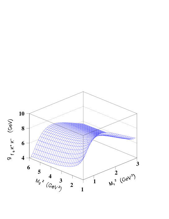
Figure 1: Coupling $g_{f_{0}K^{+}K^{-}}$ as a function of the Borel parameters $M_{1}^{2}$ and $M_{2}^{2}$, for $s_{0}=1.1$ GeV².

The result for $g_{f_{0}K^{+}K^{-}}$ versus the Borel parameters $M_{1}^{2}$ and $M_{2}^{2}$ is depicted in fig.1. A stability region where the outcome does not depend on $M_{i}^{2}$ can be selected. Such a region does not correspond to the line $M_{1}^{2}=M_{2}^{2}$, but to the range $0.8\leq M_{1}^{2}\leq 1.6$ GeV² with $M_{2}^{2}$ extending up to $M_{2}^{2}\simeq 5$ GeV². Varying $M_{1}^{2}$ and $M_{2}^{2}$ in this region, and changing the values of the thresholds and of the other parameters, we obtain the result depicted in fig.2, which can be quoted as $6.2\leq g_{f_{0}K^{+}K^{-}}\leq 7.8$ GeV.

Let us briefly discuss the uncertainties affecting the numerical result. As for the $SU(3)_{F}$ breaking effects rendering the kaon distribution amplitudes asymmetric with respect to the middle point, the neglect should have a minor role in our approach, due to the possibility of exploring wide ranges of the variable $u$ and smoothing the effects of the actual shapes of the wave functions. Another uncertainty is related to the value of the strange quark mass, $m_{s}$; since the dependence of the sum rule on $m_{s}$ mainly involves the ratio $M_{K}^{2}/m_{s}$, one can fix this ratio using chiral perturbation theory, obtaining results in the same range quoted for $g_{f_{0}K^{+}K^{-}}$.

We can compare now our result with the available experimental determinations of $g_{f_{0}K^{+}K^{-}}$, as well as with the results of other calculations. We shall see how complex the scenario is.

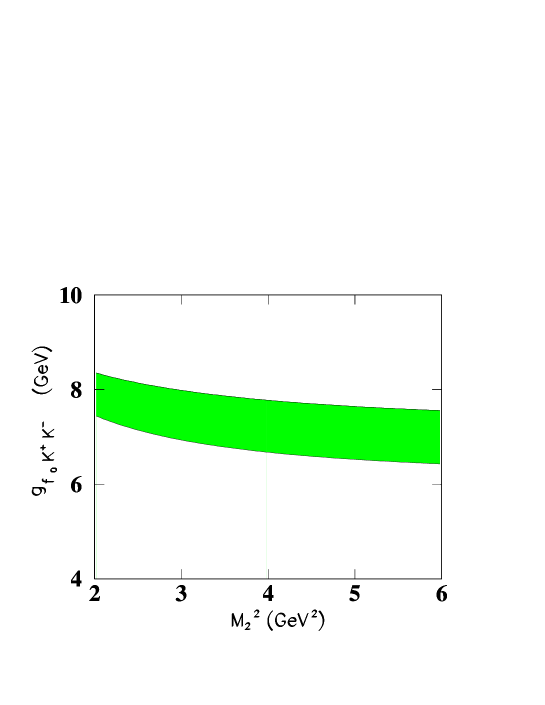
Figure 2: Coupling $g_{f_{0}K^{+}K^{-}}$ as a function of the Borel parameter $M_{2}^{2}$, varying $s_{0}$ in the range $1.05\leq s_{0}\leq 1.15$ GeV² and $M_{1}^{2}$ in the range $0.7\leq M_{1}^{2}\leq 2.0$ GeV².

3 Other determinations of $g_{f_{0}K^{+}K^{-}}$

As discussed in the Introduction, $g_{f_{0}K^{+}K^{-}}$ can be considered in connection with the radiative $\phi\to f_{0}\gamma$ decay mode. Several analyses go through this decay channel. KLOE Collaboration at the DA$\Phi$NE collider in Frascati has examined the decay channel $\phi\to\pi^{0}\pi^{0}\gamma$ measuring the branching fraction: ${\cal B}(\phi\to\pi^{0}\pi^{0}\gamma)=(1.09\pm 0.03_{stat}\pm 0.05_{syst})\times 10^{-4}$ [32]. The decay mode is supposed to proceed through $\rho\pi$ intermediate state and through kaon loop processes, with the kaons annihilating into scalar resonances that subsequently decay to $\pi^{0}\pi^{0}$. Different fits of the two pion invariant mass spectrum $\displaystyle{d\Gamma\over dM_{\pi\pi}}$ are performed in order to measure the parameters of the scalar states. In a first fit (A) only the contribution of the intermediate state $f_{0}(980)$ is considered, and the three parameters $M_{f_{0}},~{}g^{2}_{f_{0}K^{+}K^{-}}$ and $g^{2}_{f_{0}K^{+}K^{-}}/g^{2}_{f_{0}\pi\pi}$ are determined. In a second fit (B) the contribution of a possible broad scalar $\sigma$ state is included, and the coupling $g_{\phi\sigma\gamma}$ is considered as a further parameter. It is assumed that the two pion decay modes saturate the $f_{0}$ width, and that ${\cal B}(f_{0}\to\pi^{+}\pi^{-})=2~{}{\cal B}(f_{0}\to\pi^{0}\pi^{0})$ invoking isospin symmetry. Fit A provides ${\cal B}(\phi\to f_{0}\gamma)=(3.3\pm 0.2)\times 10^{-4}$ and $\displaystyle{g^{2}_{f_{0}K^{+}K^{-}}\over(4\pi)}=1.29\pm 0.14~{}GeV^{2}$ ($\chi^{2}/{\rm ndf}=109.53/34$). Fit B gives instead: ${\cal B}(\phi\to f_{0}\gamma)=(4.47\pm 0.21)\times 10^{-4}$ and $\displaystyle{g^{2}_{f_{0}K^{+}K^{-}}\over(4\pi)}=2.79\pm 0.12~{}GeV^{2}$ ($\chi^{2}/{\rm ndf}=43.15/33$). The negative interference between the contributions of the broad $\sigma$ and the $f_{0}$ is responsible of the improvement in the accuracy of the fit. In both cases sizeable values for $g_{f_{0}K^{+}K^{-}}$ are obtained; they are reported in Table 1.

An analogous analysis has been performed by the CMD-2 Collaboration at the VEPP-2M collider in Novosibirsk. From a combined fit to the spectra of the decays $\phi\to\pi^{+}\pi^{-}\gamma$ and $\phi\to\pi^{0}\pi^{0}\gamma$, CMD-2 Collaboration obtains: ${\cal B}(\phi\to f_{0}\gamma)=(2.90\pm 0.21\pm 0.65)\times 10^{-4}$ and $\displaystyle{g^{2}_{f_{0}K^{+}K^{-}}\over(4\pi)}=1.48\pm 0.32\,\,GeV^{2}$ [33]. A similar result is quoted by the SND Collaboration at the same VEPP collider: ${\cal B}(\phi\to f_{0}\gamma)=(3.5\pm 0.3\pm^{1.3}_{0.5})\times 10^{-4}$ and $\displaystyle{g^{2}_{f_{0}K^{+}K^{-}}\over(4\pi)}=2.47^{+0.73}_{-0.51}~{}GeV^{2}$ [34].

Other determinations of $g_{f_{0}K^{+}K^{-}}$ rely on the analysis of different physical processes. Considering the central $f_{0}$ production in $pp$ collisions, the WA102 experiment at CERN gets: $\displaystyle{g^{2}_{f_{0}K^{+}K^{-}}\over(4\pi)}=0.38\pm 0.06\,\,GeV^{2}$ [35]. On the other hand, analyzing the $f_{0}$ production in $D_{s}$ decays to three pions, the Collaboration E791 at Fermilab finds a value compatible with zero [36]. These results are also reported in Table 1.

In Ref.[10] the coupling constant is evaluated for different values of the phase shift of the elastic background in the $\pi\pi\to\pi\pi$ reaction, of the ratio $R=g_{f_{0}K^{+}K^{-}}^{2}/g_{f_{0}\pi^{+}\pi^{-}}^{2}$ and according to different scenarios for the $f_{0}$ structure, obtaining results in a wide range: $g_{f_{0}K^{+}K^{-}}\in[1.95,7.3]$ GeV.

The analysis of the decay channel $J/\psi\to\phi K{\overline{K}}(\pi\pi)$ has been carried out in Ref.[37]. The $f_{0}$ pole is described as a Breit-Wigner resonance coupled to two channels. Two fits of the experimental data are performed depending upon the $\pi\pi$ phase shift data used, obtaining $g_{f_{0}K^{+}K^{-}}=2.5\pm 0.15$ GeV and $g_{f_{0}K^{+}K^{-}}=2.0\pm 0.06$ GeV, respectively.

A prediction for $\displaystyle{g_{f_{0}K^{+}K^{-}}}$ based on chiral symmetry and the linear sigma model, when no mixing with the $\sigma$ is considered, is: $g_{f_{0}K^{+}K^{-}}=2.24$ GeV [38], to be compared to old determinations $g_{f_{0}K^{+}K^{-}}=2.74$ GeV [39]. Using the method of the T-matrices, the value $g_{f_{0}K^{+}K^{-}}=3.8$ GeV is obtained [40].

Considering all the above results one sees that a general consensus on $g_{f_{0}K^{+}K^{-}}$ has not been reached, so far. In particular, experimental analyses of different processes produce contradicting results. The outcome from $\phi\to f_{0}\gamma$ points towards sizeable values of the coupling, consistent with the light-cone sum rule result. One has to say that the error quoted for the experimental determinations, which in general looks small, mainly accounts for the statistical uncertainties; one could infer the size of the systematical uncertainties comparing different determinations.

As for $g_{f_{0}K^{+}K^{-}}$ from $D_{s}$ decays, presumably the determination will be improved at the B factories by experiments such as BaBar at SLAC, thanks to large available samples of $D_{s}$ mesons. In these measurements $g_{f_{0}K^{+}K^{-}}$ is expected to be determined by coupled channel analyses, with $D_{s}$ decaying to final states containing kaons as well as pions [41].

Table 1: Experimental determinations of $g_{f_{0}K^{+}K^{-}}$ using different physical processes. Double items refer to two different fits (see text).

Collaboration	process	$g_{f_{0}K^{+}K^{-}}\,(GeV)$	Ref.
KLOE	$\phi\to f_{0}\gamma\,(A)$	$4.0\pm 0.2\,(A)$	[32]
	$\phi\to f_{0}\gamma\,(B)$	$5.9\pm 0.1\,(B)$
CMD-2	$\phi\to f_{0}\gamma$	$4.3\pm 0.5$	[33]
SND	$\phi\to f_{0}\gamma$	$5.6\pm 0.8$	[34]
WA102	$pp$	$2.2\pm 0.2$	[35]
E791	$D_{s}\to 3\pi$	$0.5\pm 0.6$	[36]

4 Conclusions

The purpose of this paper was the evaluation of the strong coupling constant $g_{f_{0}K^{+}K^{-}}$, the value of which is rather controversial, as it emerges comparing different experimental and theoretical determinations. In particular, the KLOE Collaboration measured a larger value than in other determinations, with a greater accuracy as well. However, such a result stems from the investigation of $\phi\to f_{0}\gamma$, and therefore it is mandatory to wait for the study of unrelated processes, namely the combined analysis of $D_{s}$ decays to pions and kaons. The outcome of light-cone QCD sum rules is in keeping with a large value for the coupling. The uncertainty affecting the result is intrinsic of the method and does not allow a better comparison with data. However, the analysis confirms a peculiar aspect of the scalar states, i.e. their large hadronic couplings, thus pointing towards a scenario in which the process of hadronic dressing is favoured.

Acknowledgments We thank A. Palano, T. Aliev and M.E. Boglione for discussions. We acknowledge partial support from the EC Contract No. HPRN-CT-2002-00311 (EURIDICE).

References

[1]
For reviews see:
L. Montanet,
Rep. Prog. Phys. 46 (1983) 337;
F.E. Close,
Rep. Prog. Phys. 51 (1988) 833;
N.N. Achasov,
Nucl. Phys. Proc. Suppl. 21 (1991) 189;
M. R. Pennington, Proceedings of HADRON ’95, M.C. Birse, G.D. Lafferty,
J.A. McGovern eds., World Scientific (1996) page 3;
T. Barnes,
hep-ph/0001326.
[2]
F. E. Close and N. A. Tornqvist,
J. Phys. G 28 (2002) R249.
[3]
C. J. Morningstar and M. J. Peardon,
Phys. Rev. D 60 (1999) 034509;
S. Narison,
Nucl. Phys. A 675 (2000) 54C.
[4]
F. E. Close, Y. L. Dokshitzer, V. N. Gribov, V. A. Khoze and
M. G. Ryskin,
Phys. Lett. B 319 (1993) 291.
[5]
N.A. Tornqvist,
Phys. Rev. Lett. 49 (1982) 624.
[6]
N.A. Tornqvist,
Z. Phys. C 68 (1995) 647.
[7]
N.A. Tornqvist and M. Roos,
Phys. Rev. Lett. 76 (1996) 1575.
[8]
E. van Beveren et al.,
Z. Phys. C 30 (1986) 615;
M.D. Scadron,
Phys. Rev. D 26 (1982) 239;
E. van Beveren, G. Rupp and M.D. Scadron,
Phys. Lett. B 495 (2000) 300.
[9]
R.L. Jaffe,
Phys. Rev. D 15 (1977) 267, 281; D 17 (1978) 1444;
R.L. Jaffe and K. Johnson,
Phys. Lett. B 60 (1976) 201.
[10]
N.N. Achasov and V.N. Ivanchenko,
Nucl. Phys. B 315 (1989) 465;
N.N. Achasov and V.V. Gubin,
Phys. Rev. D 56 (1997) 4084.
[11]
J. Weinstein and N. Isgur,
Phys. Rev. Lett. 48 (1982) 659;
Phys. Rev. D 27 (1983) 588;
Phys. Rev. D 41 (1990) 2236.
[12]
N. Brown and F.E. Close, in The DANE Physics HandBook,
L. Maiani, G. Pancheri and N. Paver eds, INFN Frascati, 1995, pp.
447-464;
F.E. Close, N. Isgur and S. Kumano,
Nucl. Phys. B 389 (1993) 513.
[13]
R. Kaminski, L. Lesniak and J.P. Maillet,
Phys. Rev. D 50 (1994) 3145.
[14]
N.N. Achasov, V.V. Gubin and V.I. Shevchenko,
Phys. Rev. D 56 (1997) 203.
[15]
N. A. Tornqvist,
arXiv:hep-ph/0204215.
[16]
M. Boglione and M. R. Pennington,
Phys. Rev. Lett. 79 (1997) 1998.
[17]
N. A. Tornqvist,
arXiv:hep-ph/0008136.
[18]
C. M. Shakin and H. Wang,
Phys. Rev. D 63 (2001) 014019.
[19]
F. De Fazio and M. R. Pennington,
Phys. Lett. B 521 (2001) 15.
[20]
M. Boglione and M. R. Pennington,
Phys. Rev. D 65 (2002) 114010.
[21]
F. E. Close and A. Kirk,
Phys. Lett. B 515 (2001) 13.
[22]
I. I. Balitsky, V. M. Braun and A. V. Kolesnichenko,
Nucl. Phys. B 312 (1989) 509;
V. L. Chernyak and I. R. Zhitnitsky,
Nucl. Phys. B 345 (1990) 137.
[23]
For a recent review of the method see: P. Colangelo and A. Khodjamirian,
in ”At the Frontier of Particle Physics”, vol. 3, M.
Shifman ed., World Scientific (2001), page 1495.
[24]
T. M. Aliev, A. Ozpineci and M. Savci,
Phys. Lett. B 527 (2002) 193.
[25]
T-products of quark currents between the vacuum and one-particle states
were first investigated in
N. S. Craigie and J. Stern,
Nucl. Phys. B 216 (1983) 209.
[26]
S. Narison,
Nucl. Phys. B 509 (1998) 312.
[27]
V. M. Belyaev, V. M. Braun, A. Khodjamirian and R. Rückl,
Phys. Rev. D 51 (1995) 6177.
[28]
V. M. Braun and I. E. Halperin,
Z. Phys. C 48 (1990) 239.
[29]
P. Ball,
JHEP 9901 (1999) 010.
[30]
P. Colangelo, F. De Fazio, G. Nardulli and N. Paver,
Phys. Lett. B 408 (1997) 340;
K. Maltman and J. Kambor,
Phys. Rev. D 65 (2002) 074013;
M. Jamin, J. A. Oller and A. Pich,
Eur. Phys. J. C 24 (2002) 237.
[31]
A.A. Ovchinnikov and A.Pivovarov, Phys. Lett. B 163 (1985) 231.
[32]
A. Aloisio et al. [KLOE Collaboration],
Phys. Lett. B 537 (2002) 21.
[33]
R. R. Akhmetshin et al. [CMD-2 Collaboration],
Phys. Lett. B 462 (1999) 380;
Nucl. Phys. A 675 (2000) 424C.
[34]
M. N. Achasov et al.,
Phys. Lett. B 485 (2000) 349.
[35]
D. Barberis et al. [WA102 Collaboration],
Phys. Lett. B 462 (1999) 462.
[36]
E. M. Aitala et al. [E791 Collaboration],
Phys. Rev. Lett. 86 (2001) 765.
[37]
R. Escribano, A. Gallegos, J. L. Lucio M, G. Moreno and
J. Pestieau,
arXiv:hep-ph/0204338.
[38]
M. Napsuciale,
arXiv:hep-ph/9803396;
J. L. Lucio Martinez and M. Napsuciale,
Phys. Lett. B 454 (1999) 365.
[39]
J. F. Donoghue, B. R. Holstein and G. Valencia,
Phys. Rev. D 35 (1987) 2769;
G. Ecker, A. Pich and E. de Rafael,
Phys. Lett. B 189 (1987) 363;
G. Ecker, A. Pich and E. de Rafael,
Nucl. Phys. B 303 (1988) 665;
L. M. Sehgal,
Phys. Rev. D 38 (1988) 808;
S. Nussinov and T. N. Truong,
Phys. Rev. Lett. 63 (1989) 1349 [Erratum-ibid. 63 (1989) 2002];
J. L. Lucio Martinez and J. Pestieau,
Phys. Rev. D 42 (1990) 3253.
[40]
J. A. Oller and E. Oset,
Nucl. Phys. A 620 (1997) 438 [Erratum-ibid. A 652
(1999) 407];
J. A. Oller,
arXiv:hep-ph/0205121.