Estimating the inelasticity with the information theory approach

Abstract

Using the information theory approach, in both its extensive and nonextensive versions, we estimate the inelasticity parameter $K$ of hadronic reactions together with its distribution and energy dependence from $p\bar{p}$ and $pp$ data. We find that the inelasticity remains essentially constant in energy except for a variation around $K\sim 0.5$, as was originally expected.

PACS numbers: 96.40 De, 13.85.Tp, 96.40.Pg, 13.85.Ni

1 Introduction

The inelasticity $K$ ($0<K<1$) of a reaction has well established importance in working with data from cosmic ray cascades [1] (cf. also [2, 3, 4] and references therein). It tells us what fraction of the energy of a projectile is used for production of secondaries and what fraction flows further along the cascade chain. In cosmic ray observables, $K$ in fact appears in some combination which also contains the mean free path for the particle propagation in the atmosphere, or equivalently, the total inelastic cross section $\sigma_{in}$. This makes $K$ difficult to estimate because of the freedom available to attribute the observed effects either to $K(s)$ or to $\sigma(s)$. It was therefore proposed in [1] that in order to extract $K(s)$ unambiguously from cosmic ray experiments one should analyse simultaneously the data from (at least) two different types of experiments for which combinations of $K$ and $\sigma_{in}$ are different [5].

Nowadays there is a strong tendency to replace inelasticity and simple energy flow models by more refined and complicated models of multiparticle production (see [7, 8, 9] and references therein). In their present formulations such models differ substantially among themselves, concerning both their physical basis and the (usually very large) number of parameters used, and lead to quite different, sometimes even contradictory, predictions [8, 9]. While developing models is necessary for the global understanding of cosmic ray physics, for the purpose of studying energy flow it may be desirable to have a more economical description of high energy collisions, involving only a small number of parameters. This is one of the advantages of working with the concept of inelasticity [1, 10].

The inelasticity is also a very important quantity in phenomenological descriptions of hadronic and nuclear collisions in terms of statistical models of multiparticle production processes [11, 12]. In this case it enters either explicitly, as a single parameter $K$ defining the initial energy $M=K\cdot\sqrt{s}$ to be hadronized, or implicitly, when one finds that out of numerous parameters of the model only the combination leading to the given fraction of available energy to be converted into produced secondaries, $K\cdot\sqrt{s}$, is important, see [13]. Attempts to estimate it are thus fully justifiable. In [11, 12] the calculations of the inelasticity distribution, $\chi(K)$ (and its energy dependence), based on the assumed dominance of high energy multiparticle processes by gluonic interactions, was presented. In the other calculations the mean inelasticity $K$ and its possible energy dependence was simply estimated either by using thermal-like model formulas applied to collider $\bar{p}p$ data [14, 15, 16, 17, 18] (like, for example, in [19]) or by some other means [20].

In this paper we address this problem again, this time by means of the information theory approach both in its extensive [21] and nonextensive [22, 23] versions. The idea is to describe the available data by using only a truly minimal amount of information avoiding therefore any unfounded and unnecessary assumptions. This is done by attributing to the measured distributions (written in terms of the suitable probability distributions) an information entropy $S$ and maximizing it subject to constraints which account for our a priori knowledge of the process under consideration. As a result one gets the most probable and least biased distribution describing these data, which is not influenced by anything else besides the available information. In such approach the inelasticity $K$ emerges as the only real parameter; all other quantities being well defined functions of it. We attempt to clarify here the role of the inelasticity by using both the extensive and nonextensive versions of information theory. All necessary background on the information theory approach needed in the present context is given in the next Section. Section 3 contains our results for the $p\bar{p}$ and $pp$ collisions. Our conclusions and summary are presented in the last Section.

2 General ideas of information theory approach

As presented at length in [21] (where further details and references can be found) the information theory approach provides us, by definition, with the most probable, least biased estimation of a probability distribution $\{p_{i},i=1,\dots,n\}$ using only knowledge of a finite number of observables $\{F_{k},k=1,\dots,n\}$ of some physical quantities obtained by means of $p_{i}$ and defined as:

$$F_{k}=\langle{F}_{k}\rangle=\sum_{i=1}^{n}p_{i}\,{F}_{k}^{(i)}.$$ (1)

One is looking for such $\{p_{i}\}$ which contain only information provided by $\{F_{k}\}$ and nothing more, i.e., which contain minimal information. The information connected with $\{p_{i}\}$ is quantified by the Shannon information entropy defined as:

$$S\,=\,-\Sigma_{i}p_{i}\ln p_{i}.$$ (2)

Minimum information corresponds to maximum entropy $S$, therefore the $\{p_{i}\}$ we are looking for are obtained by maximizing the information entropy $S$ under conditions imposed by the measured observables $\{F_{k}\}$ as given by eq.(1). They result in a set of Lagrange multipliers $\{\lambda_{k},k=1,\dots,r\}$ and the generic form of $\{p_{i}\}$ we are looking for is [21]:

$$p_{i}=\frac{1}{Z}\,\exp\left[-\sum_{k=1}^{r}\,\lambda_{k}\cdot F_{k}^{(i)}\right],$$ (3)

where $Z$ is obtained from the normalization condition $\sum_{i=1}^{n}p_{i}=1$.

Such approach was applied long time ago to experimental data on multiparticle production with the aim at establishing the minimum amount of information needed to describe them [13]. The rationale was to understand what makes all the apparently disparate (if not outright contradictory) models of that period fit (equally well) the data. The result was striking and very instructive [13]: the data considered (multiplicity and momentum distributions) contained only very limited amount of information, which could be expressed in the form of the following two observations: $(i)$ the available phase space in which particles are produced is limited (i.e., there is some sort of $p_{T}$ cut-off) and $(ii)$ only a part $K\in(0,1)$ of the available energy $\sqrt{s}$ is used to produce the observed secondaries, the rest being taken away by the so called leading particles (i.e., inelasticity emerges as one of the cornerstone characteristics of reaction). All other assumptions, different for different models (based on different, sometimes even contradictory, physical pictures of the collision process) were therefore spurious and as such they could be safely dropped out without spoiling the agreement with experimental data. In fact, closer scrutiny of these models showed that they all contained, explicitly or implicitly, precisely those two assumptions mentioned above and that was the true reason of their agreement with data.

In this paper we are therefore following the same line of approach with the aim at deducing from the available data for the inelasticity parameter $K$. Notice that the formula (3) resembles the statistical model formulas based on the Boltzmann-Gibbs statistics as used in [19]. However, in (3) no thermal equilibrium is assumed and all $\lambda_{k}$ (i.e., among others also the ”partition temperature” $T$ in [19]) are given by the corresponding constraint equation (1) whereas normalization fixes $Z$, which is a free parameter in [19].

This approach can be generalized to systems which cannot be described by Boltzmann-Gibbs (BG) statistics because of either the existence of some sort of long-range correlations (or memory) effects or fractal structure of their phase space or because of the existence of some intrinsic fluctuations in the system under consideration. It turns out that such systems are nonextensive and therefore must be described by a nonextensive generalization of BG statistics, for example by the so called Tsallis statistics [22] defined by the following form of the entropy:

$$S_{q}\,=\,-\frac{1}{1-q}\Sigma_{i}\left(1-p_{i}^{q}\right).$$ (4)

It is characterized by the nonextensivity parameter $q$ such that for two independent systems $A$ and $B$

$$S_{q(A+B)}=S_{qA}+S_{qB}+(1-q)S_{qA}S_{qB}.$$ (5)

Notice that in the limit $q\rightarrow 1$ one recovers the previous form of Boltzmann-Gibbs-Shannon entropy (2). Maximazing $S_{q}$ under constraints, which are now given in the form [24]:

$$F^{(q)}_{k}=\langle{F}_{k}\rangle_{q}=\sum_{i=1}^{n}[p_{i}]^{q}\,{F}^{(q,i)}_{k},$$ (6)

results in the following power-like form of the (most probable, least biased) probability distribution:

$$p_{i}\,=\,p^{(q)}_{i}\,=\,\frac{1}{Z_{q}}\,\exp_{q}\left[-\sum_{k=1}^{r}\,\lambda_{k}\cdot F^{(q,i)}_{k}\right],$$ (7)

where $Z_{q}$ is obtained from the normalization condition $\sum_{i=1}^{n}p^{(q)}_{i}=1$. and where

$$\exp_{q}\left(-\frac{x}{\Lambda}\right)\stackrel{{\scriptstyle\it def}}{{=}}\left[1-(1-q)\left(\frac{x}{\Lambda}\right)\right]^{\frac{1}{1-q}}.$$ (8)

Of special interest to us here will be the fact that intrinsic fluctuations in the system, represented by fluctuations in the parameter $1/\Lambda$ in the exponential distribution of the form $\sim\exp(-x/\Lambda)$ result in its nonextensivity with parameter $q$ given by a normalized variation of fluctuation of the parameter $1/\Lambda$ [23]:

$$q=1\pm\frac{\left\langle\left(\frac{1}{\Lambda}\right)^{2}\right\rangle-\left\langle\frac{1}{\Lambda}\right\rangle^{2}}{\left\langle\frac{1}{\Lambda}\right\rangle^{2}}.$$ (9)

So far this has been proven only for fluctuations of $1/\Lambda$ given in the form of the gamma distribution,

$$f\left(\frac{1}{\Lambda}\right)=\frac{\mu}{\Gamma(\alpha)}\left(\frac{\mu}{\Lambda}\right)^{\alpha-1}\exp\left(-\frac{\mu}{\Lambda}\right),$$ (10)

but this conjecture seems to be valid also in general [27] .

3 Inelasticity obtained from analysis of the $\bar{p}p$ collider and $pp$ fixed target data

The available information in this case consists of:

• The mean multiplicity of charged secondaries, $\langle n_{ch}\rangle$, produced in nonsingle diffractive reactions at given energy $\sqrt{s}$, which can be parametrized as $\langle n_{ch}\rangle=A+B\ln s+C\ln^{2}s$ or as $\langle n_{ch}\rangle=D+Es^{\gamma}$ (see [28]). In what follows we shall assume, for simplicity, that they are pions with mass $\mu=0.14$ GeV. Out of it, we shall construct and use the total mean number of produced particles assuming it to be $N=\frac{3}{2}\langle n_{ch}(s)\rangle$.

• The observation that the phase space filled by the produced secondaries is essentially one-dimensional with limited (and only slowly growing with energy) transverse momenta [29]: $\langle p_{T}\rangle=0.3+0.044\ln\left(\frac{\sqrt{s}}{20}\right)$ [30].

• The rapidity distributions of charged secondaries, $dN(s)/dy=\int d^{2}p_{T}\frac{dN}{d^{3}p}$, provided either by collider experiments [14, 15, 16, 17] or by the fixed target experiment [31]. They are available only in a limited range of the rapidity space, depending on the details of the experimental setup [29].

Following the results obtained in [13] we expect (and therefore assume in what follows) that only a part $W=K\sqrt{s}$ of the total energy $\sqrt{s}$ is used to produce secondaries in the central region of the investigated reaction. The inelasticity $K=K(s)$ will therefore be the main quantity we shall investigate.

We start with the information theory approach in its extensive version. In this case the relevant probability distribution defining information entropy (2) is given by

$$p(y)=p(y;N,W=K\sqrt{s})=\frac{1}{N}\cdot\frac{dN}{dy}$$ (11)

whereas constraint (1) is just the energy conservation (here $\mu_{T}=\sqrt{\mu^{2}+\langle p_{T}\rangle^{2}}$ and $\langle E\rangle$ is the mean energy per produced particle) [33]:

$$\int_{-Y_{m}}^{Y_{m}}\,dy\,\left[\mu_{T}\,\cosh y\right]\,p(y)=\frac{W}{N}=\langle E\rangle=\frac{K\cdot\sqrt{s}}{N}.$$ (12)

The limits of the relevant longitudinal phase space are

$$Y_{m}=\ln\left\{\frac{W^{\prime}}{2\mu_{T}}\left[1+\left(1-\frac{4\mu^{2}_{T}}{W^{\prime 2}}\right)^{\frac{1}{2}}\right]\right\},\qquad W^{\prime}=W-(N-2)\mu_{T}.$$ (13)

We would like to stress that throughout this paper the central region of the reaction, i.e., the region populated by produced particles distributed according to $p(y)$ (or $p_{q}(y)$ later on), is always defined by eq. (13). Therefore $y\in\left(-Y_{m},Y_{m}\right)$ in the CMS and we do not choose arbitrary cuts in rapidity space (as, for example, in [13]). Following now the steps mentioned in Section 2, i.e., minimazing the respective information entropy (2) with the constraint given by (12), we arrive at [21]:

$$p(y)=\frac{1}{N}\frac{dN(y)}{dy}=\frac{1}{Z}\,\exp\left(-\beta\mu_{T}\cosh y\right)$$ (14)

with $\beta=\beta(W,N,\mu_{T})$ given by solving eq. (12) and

$$Z=Z(W,N,\mu_{t})=\int^{Y_{m}}_{-Y_{m}}\,dy\exp\left(-\beta\mu_{T}\cosh y\right)$$ (15)

given by the normalization condition, $\int dyp(y)=1$. Notice that in such an approach the ”inverse temperature” $\beta$ and the normalization $Z$ depend on our input information, i.e., on $N$ and $\mu_{T}$, and on the assumed inelasticity $K$ (via $W=K\cdot\sqrt{s}$), which is our free parameter. They are therefore maximally correlated which means that the shape of distribution $p(y)$ (given by $\beta$) and its height (given by $Z$) are not independent of each other. This is in sharp contrast to the approaches presented before in [19] where both $\beta$ (called ”partition temperature”) and the normalization (our $Z$) were treated as two independent parameters. Because of the symmetry of the colliding system momentum conservation does not impose any additional constraint here and we are left with $\beta$ being the only Lagrange multiplier to be calculated from eq.(12) for each energy $W$ and multiplicity $N$.

Notice that (14), although formally resembling formulae obtained in thermal models [32], has a much wider range of applicability as it is not connected with any assumption of thermal equilibrium. Actually it can be written in the scaling-like form:

$$p(y)\,=\,\frac{1}{Z}\exp\left[-\bar{\beta}\cdot\frac{\mu_{T}\cosh y}{\langle E\rangle}\right],$$ (16)

where $\langle E\rangle=W/N$ is the mean energy per produced particle and $\bar{\beta}=\beta\cdot W/N$. Plotting $\bar{\beta}$ as a function of $\langle E\rangle$ one observes that for the minimal number of produced secondaries ($N\rightarrow 2$) $\bar{\beta}\rightarrow-\infty$, whereas for the maximal number ($N\rightarrow N_{max}=W/\mu_{T}$) $\bar{\beta}\rightarrow+\infty$. There is also an intermediate region in which $\bar{\beta}$ remains fairly constant leading to an approximate ”plateau” in $p(y)$. In this region ”partition temperature” $1/\beta$ and inelasticity $K$ are related in a very simple way, namely

$$\beta\,\simeq\,\frac{N}{K\cdot\sqrt{s}}.$$ (17)

Actually, $\beta>0$ only for $N>N_{0}=2\ln\left(N_{max}\right)$ and ”plateau” occurs only for $N\simeq N_{0}$. It clearly shows that $T=1/\beta$, called sometimes ”partition temperature” [19], is a measure of energy available per produced particle (which therefore depends also on inelasticity).

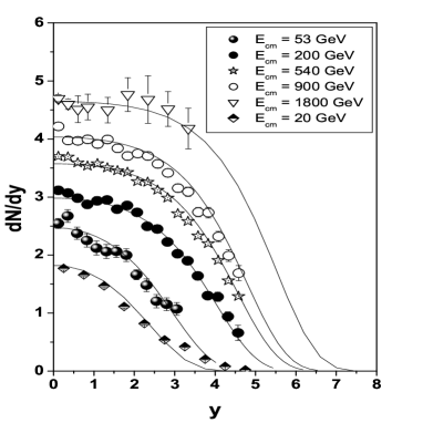
Figure 1: Rapidity spectra obtained by UA5 [14] and Tevatron [15] fitted by formula (14). For completeness results for $pp$ data at $20$ GeV [31] are also shown. The corresponding values of inelasticity $K$ are listed in Table 1.

Figure 2: Rapidity spectra obtained by UA5 [14] and Tevatron [15] fitted by formula (19). For completeness results for $pp$ data at $20$ GeV [31] are also shown. The corresponding values of $q-$inelasticity $\kappa_{q}$ and nonextensivity parameter $q$ are listed in Table 1.

In the case of the nonextensive version of information entropy the energy conservation constraint is given by

$$\int_{-Y_{m}}^{Y_{m}}\,dy\,\left[\mu_{T}\,\cosh y\right]\,[p_{q}(y)]^{q}=\frac{W_{q}}{N}=\frac{\kappa_{q}\cdot\sqrt{s}}{N}.$$ (18)

and maximization of the corresponding Tsallis entropy (4) results in

$$p_{q}(y)=\frac{1}{N}\frac{dN_{q}}{dy}=\frac{1}{Z_{q}}\exp_{q}\left(-\beta_{q}\mu_{T}\cosh y\right)$$ (19)

(where $\exp_{q}(...)$ is defined by eq. (8) and $Z_{q}$ is given, as in (15), by the normalization condition, $\int dyp_{q}(y)=1$). The characteristic feature of $p_{q}(y)$, as shown in Fig. 6, is that it enhances (depletes) the tails of the distribution for $q>1$ ($q<1$), respectively (or, in other words, it enhances or depletes the more or, respectively, less probable events). Notice that in this case, differently than in (14), one has to be sure that $1-(1-q)\beta_{q}\mu_{T}\cosh y\geq 0$, which imposes an additional condition on the allowed phase space for $q<1$ and $\beta_{q}>0$. In this case the strict correlation between the shape of rapidity distribution and its height is relaxed because both depend also on the new parameter $q$. This fact will be important later on. The scaling-like formula (16) and the approximate relation (17), this time between $\beta_{q}$ and $\kappa_{q}$, are still valid, albeit this time only approximately, i.e., for small values of $|q-1|$. On the other hand $\beta_{q}>0$ for $N=\left(2\ln N_{max}\right)^{q}$, i.e., for larger (smaller) multiplicities, depending whether $q>1$ ($q<1$).

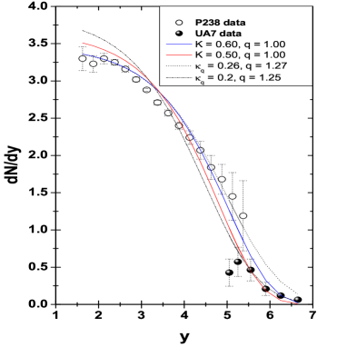
Figure 3: Comparison of data for rapidity distributions at $\sqrt{s}=630$ GeV obtained by P238 [16] (open circles) and UA7 [17] collaborations (full circles) with predictions of our model for it extensive ($q=1$) and nonextensive versions. Notice that one can fit at the same time either P238 or UA7 data but not both together.

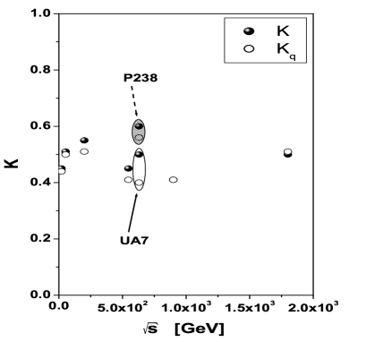
Figure 4: Energy dependences of inelasticities obtained in extensive ($K$, see (12)) and nonextensive ($K_{q}$, see (3)) approaches (cf. also Table 1). Notice that results for P238 data do not follow the overall trend (see text).

The results for fits using extensive formula (14) are displayed in Fig. 2 and those using its nonextensive version given by eq. (19) are shown in Fig. 2. As one can see they are almost identical, differences are showing up only for $20$ GeV where data develop a tail which is most sensitive to the parameter $q$. The result for the joint distributions of UA7 data from [17] and P238 [16] data at $630$ GeV are shown separately in Fig. 4. Both sets of data are clearly incompatible in the sense that UA7 data (which are for $\pi^{0}$’s and have been taken here in the same way as in [34]) do not continue the trend shown by P238 data (which are, as UA5 ones, for charged particles). Instead they seem to continue the trend of the charged UA5 data, which is also clearly seen from the values of the obtained parameters displayed in Table 1. Because of this fact we have fitted them separately. The results for the respective inelasticity parameter $K$ and its $q$-equivalent $\kappa_{q}$ for different energies are shown in Table 1. The estimated errors (the same for both approaches) range from $\Delta K=0.02$ for $20$ GeV (where the fitted range in rapidity is biggest) to $\Delta K=0.05$ for $1800$ GeV (where the lack of measured tails prevents a better fit). These errors should be kept in mind when looking at Fig. 4, which summarizes the obtained inelasticities of different types. These inelasticities can be compared with inelasticities $K_{|y|\leq 4}$ defined by the formula

$$K_{|y|\leq 4}=\frac{N}{\sqrt{s}}\int^{Y_{m}=4}_{Y_{m}=-4}\!dy\ p(y)[\mu_{T}\cosh y],$$ (20)

i.e., in the same way as in [19], namely, by integrating over the same part of the phase space limited by $|Y_{m}|=4$. Notice that values of $K_{|y|\leq 4}$ are systematically smaller than the corresponding values of $K$ and are in a visible way decreasing with energy. The reason for such behaviour is that $K_{|y|\leq 4}$ counts the fraction of energy in a fixed domain in the phase space given by the condition that $|y|\leq 4$ whereas our $K$ gives the energy used for production of particles in the whole kinematically allowed region $|y|\leq Y_{m}$ as defined by eq. (13). Table 1 contains also the corresponding values of the ”partition temperature” $T=\frac{1}{\beta}$ obtained from the eq. (12).

$\sqrt{s}$	$\langle n_{ch}\rangle$	$\langle p_{T}\rangle$	$K$	$T$	$K_{|y|\leq 4}$	$q$	$\kappa_{q}$	$\tau_{q}$	$K_{q}$	$K_{q}^{(|y|\leq 4)}$
(GeV)		(GeV)		(GeV)				(GeV)
20	$7.7$	0.30	$0.45$	$1.76$	$0.53$	$1.05$	$0.40$	$2.07$	$0.44$	$0.60$
53	$13.0$	0.34	$0.51$	$3.53$	$0.50$	$1.13$	$0.38$	$4.06$	$0.50$	$0.57$
200	$21.4$	0.40	$0.55$	$12.12$	$0.37$	$1.20$	$0.30$	$11.74$	$0.51$	$0.37$
540	$29.1$	0.45	$0.45$	$22.38$	$0.22$	$1.26$	$0.20$	$20.39$	$0.41$	$0.22$
(a)630	$31.0$	0.45	$0.60$	$36.29$	$0.22$	$1.27$	$0.26$	$35.51$	$0.56$	$0.22$
(b)630	$31.0$	0.45	$0.50$	$28.90$	$0.21$	$1.25$	$0.20$	$21.22$	$0.40$	$0.21$
900	$34.6$	0.48	$0.41$	$29.47$	$0.17$	$1.29$	$0.18$	$30.79$	$0.41$	$0.17$
1800	$46.4$	0.50	$0.50$	$55.69$	$0.13$	$1.33$	$0.19$	$62.57$	$0.51$	$0.13$

Table 1: The results for extensive (eqs. (14)) and nonextensive (eq. (19)) approaches applied to $pp$ [31] and $p\bar{p}$ data [14, 15, 16, 17] on rapidity distributions. The first three columns summarize our input information: energy $\sqrt{s}$, total charge multiplicities $\langle n_{ch}\rangle$ (estimated as in [28]) and $\langle p_{T}\rangle$ (estimated as in [29]). Presented are extensive inelasticity $K$ and parameters $\kappa_{q}$ and $q$ out of which the nonextensive inelasticity $K_{q}$ is calculated by means of (3)). For completeness the corresponding ”partition temperatures” $T=1/\beta$ and $\tau_{q}=1/\beta_{q}$ are also listed as well as the corresponding inelasticities obtained for the limited portion of the phase space: $K_{|y|\leq 4}$ as given by eq. (20) and $K_{q}^{(|y|\leq 4)}$ as defined by (22). For $\sqrt{s}=630$ GeV we display separately results from fitting $(a)$ P238 data [16] and $(b)$ UA7 data [17].

In what concerns the nonextensive approach one must realize that parameter $\kappa_{q}$ occurring in (18) is not the inelasticity in the same sense as $K$ from the extensive approach, cf. eq. (12). The reason is simple (and shown in best way in [35] where Hagedorn statistical model of multiparticle production [36] has been extended to $q$-statistics). Namely, because $q$ summarizes all kinds of correlations and/or fluctuations present in the system (and make it nonextensive) the energies per particle present on the rhs of eqs. (12) and (18) also contain in the nonextensive case contributions from these correlations or fluctuations, i.e., a kind of effective interaction characterized by $|q-1|$ [35, 23]. The enhanced (depleted) for $q>1$ ($q<1$) tails of $p_{q}(y)$ observed in Fig. 6 say that more (less) particles are sent there towards the end of the phase space, respectively. This fact must then be compensated by the appropriate choice of the value of ”$q$-inelasticity” parameter $\kappa_{q}$ in (18), which fixes the energy $W_{q}$ in this case. It should be also added at this point that when one is allowing the whole energy $\sqrt{s}$ to be used for the production of secondaries and uses nonextensive version of information theory to find $\frac{dN}{dy}$ then one finds $q<1$ [37], not $q>1$ as here. This is, however, expected because of the already mentioned fact that the $q<1$ case enhances frequent events whereas $q>1$ the rare ones. When considering the whole phase space it comprises all produced particles, which are located predominantly only in part of it. Therefore we have to enhance those frequent events by using $q<1$. This choice, as was mentioned above, limits also the allowed phase space. On the other hand, when $K$ is accounted for (as in the present case), the allowed phase space is essentially correctly described by $K\cdot\sqrt{s}$ and one has only to enhance the rare events when particles (because of fluctuations) ”leak out” of it, what results in $q>1$.

Figure 5: The examples of $p_{q}(y)$ as given by eq.(19) for $q=0.7$ and $q=1.3$ compared with $p(y)$ for $q=1$ as given by eq.(14) for one-dimensional hadronization of mass $M=100$ GeV into $N=20$ secondaries.

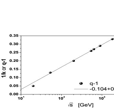
Figure 6: The values of the nonextensivity parameter $q$ obtained in fits shown in Fig. 2 (and listed in Table 1) compared with the values of the parameter $k$ of Negative Binomial distribution fit to the corresponding multiplicity distributions as given in [29], see eq.(24).

.

In order to get a nonextensive version of inelasticity, i.e., $K_{q}$, let us first observe that, according to (12), inelasticity $K$ can be expressed by the mean energy per particle, $\langle E\rangle$, therefore, in the nonextensive case one can write accordingly

$$K_{q} = \frac{N}{\sqrt{s}}\langle E\rangle_{q}\,=\,\frac{N}{\sqrt{s}}\int^{Y_{m}}_{Y_{m}}\!dy\ p_{q}(y)[\mu_{T}\cosh y],$$

$$\approx \frac{\kappa_{q}}{3-2q}.$$

(with $Y_{m}$ provided by eq. (13)). The approximate relation of $K_{q}$ with the parameters $\kappa_{q}$ and $q$ in nonextensive formula (19) arises when one estimates $\langle E\rangle_{q}$ for $|Y_{m}|\rightarrow\infty$ and uses the nonextensive version of relation (17). As it can be seen from Table 1, nonextensive inelasticity $K_{q}$ defined this way agrees reasonably well with the extensive inelasticity $K$. Notice that $K_{q}^{(|y|\leq 4)}$, defined as

$$K_{q}^{(|y|\leq 4)}=\frac{N}{\sqrt{s}}\int^{Y_{m}=4}_{Y_{m}=-4}\!dy\ p_{q}(y)[\mu_{T}\cosh y],$$ (22)

is essentially identical with $K_{|y|\leq 4}$ discussed above (and for the same reason). These results indicate that the true equivalent of inelasticity $K$ in nonextensive approach is $K_{q}$, at least in the sense used in cosmic ray research, namely that it defines the part of the initial energy taken away by leading particles: $K_{elastic}=1-K$ should be replaced by: $K_{elastic}=1-K_{q}$. They are displayed explicitly in Fig. 4. Notice that P238 data [16] at $\sqrt{s}=630$ GeV clearly do not follow the trend presented by the UA5, UA7 and Tevatron data [14, 15]. When neglecting this point the overall tendency is that inelasticity is essentially constant with energy and equal to $K\simeq 0.5$, which agrees with first estimates made in [38, 4, 20] and with first experimental estimates based on the analysis of the leading particle effect provided in [39].

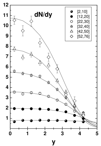
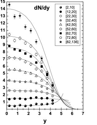
Figure 7: Fits to $\frac{dN}{dy}$ for different rapidity bins for $\sqrt{s}=200$ and $900$ GeV (left and right panels, respectively) by means of eq.(19).

A comment on the possible physical meaning of the parameter $q$ obtained from our fits and listed in Table 1 is in order here. As we said before, in general, the nonextensivity parameter $q$ summarizes the action of several factors, each of which leads to a deviation from the simple form of the extensive Boltzmann-Gibbs statistics, or Shannon entropy defined by eq.(2). Among them are the possible intrinsic fluctuations existing in the hadronizing system [23]. Notice that in the case considered here we have not accounted explicitly for the fact that each event has its own multiplicity $N$ but we have used only its mean value, $\langle N\rangle$, as given by experiment where $\langle N\rangle=\sum NP(N)$ with $P(N)$ being the multiplicity distribution. Actually, we have used only its charged part, $\langle n_{ch}\rangle$, assuming that $N=\frac{3}{2}\langle n_{ch}\rangle$, i.e., neglecting in addition also possible fluctuations between the number of charged and neutral secondaries. Experimentally it is known that $P(n_{ch})$ is adequately described by the so called Negative Binomial distribution (NBD) [29], which depends on two parameters: the mean multiplicity $\langle n_{ch}\rangle$ and the parameter $k$ ($k\geq 1$) affecting its width,

$$\frac{1}{k}\,=\,\frac{\sigma^{2}(n_{ch})}{\langle n_{ch}\rangle^{2}}\,-\,\frac{1}{\langle n_{ch}\rangle}.$$ (23)

For $k\rightarrow 1$ NB approaches a geometrical distribution whereas for $k^{-1}\rightarrow 0$ it approaches a Poissonian distribution. In general it is found [29] that

$$\frac{1}{k}=-0.104+0.058\cdot\ln\sqrt{s}.$$ (24)

Following the ideas expressed in [23] we would like to draw attention to the fact that the value of $k^{-1}$ may be also understood as the measure of fluctuations of the mean multiplicity (cf. also [40]). When there are only statistical fluctuations in the hadronizing system one should expect the Poissonian form of the corresponding multiplicity distributions. The existence of intrinsic (dynamical) fluctuations would mean that one allows the mean multiplicity $\bar{n}$ to fluctuate. In the case when such fluctuations are given by a gamma distribution with normalized variance $D(\bar{n})$ then, as a result, one obtains the Negative Binomial multiplicity distribution with

$$\frac{1}{k}\,=\,D(\bar{n})\,=\,\frac{\sigma^{2}\left(\bar{n}\right)}{\langle\bar{n}\rangle^{2}}.$$ (25)

That is because in this case (see also [41]):

$$P(n)\,=\,\int_{0}^{\infty}d\bar{n}\frac{e^{-\bar{n}}\bar{n}^{n}}{n!}\cdot\frac{\gamma^{k}\bar{n}^{k-1}e^{-\gamma\bar{n}}}{\Gamma(k)}=\frac{\Gamma(k+n)}{\Gamma(1+n)\Gamma(k)}\cdot\frac{\gamma^{k}}{(\gamma+1)^{k+n}}$$ (26)

where $\gamma=\frac{k}{\langle\bar{n}\rangle}$. Assuming now that these fluctuations contribute to nonextensivity defined by the parameter $q$, i.e., that $D(\bar{n})=q-1$ [23] one should expect that [42]

$$q\,=\,1\,+\,\frac{1}{k}.$$ (27)

As can be seen in Fig. 6 this is precisely the case. Namely, fluctuations existing in experimental data for the rapidity distributions, $dN/dy$ [14, 15, 31], and disclosed by fits using the nonextensive form (19) follow (except for the lowest energy point at $20$ GeV) the pattern of fluctuations seen in data for multiplicity distributions $P(N)$ and summarized by the parameter $k$ of NBD [29]. This means then that these data contain no more information than used here, namely existence of limited $p_{T}$, inelasticity $K$ and fluctuations as given by $q>1$ or $k^{-1}>0$.

	$\sqrt{s}=200$ GeV				$\sqrt{s}=900$ GeV
$\Delta N$
	$q$	$\kappa_{q}$	$\tau_{q}$	$K_{q}$	$q$	$\kappa_{q}$	$\tau_{q}$	$K_{q}$
			(GeV)			( GeV)
$[2,10]$	1.001	0.35	114.00	0.35	1.25	0.10	-34.20	0.16
$[12,20]$	1.10	0.41	20.99	0.54	1.26	0.17	316.55	0.33
$[22,30]$	1.14	0.44	11.00	0.64	1.27	0.20	62.63	0.42
$[32,40]$	1.17	0.45	7.31	0.72	1.27	0.22	34.98	0.48
$[42,50]$	1.18	0.46	5.10	0.75	1.23	0.25	22.74	0.50
$[52,N_{1}]$	1.25	0.50	4.39	0.98	1.21	0.26	16.28	0.49
$[62,70]$					1.20	0.31	15.79	0.57
$[72,80]$					1.20	0.33	14.02	0.61
$[82,136]$					1.22	0.38	12.00	0.74

Table 2: Results for the same parameter $q$, $\kappa_{q}$, $\tau_{q}$ and $K_{q}$ as shown and defined in Table 1 but now obtained for data taken in the restricted multiplicity bins $\Delta N$ [18] and shown in Fig. 7. Here: $N_{1}=76$ for $\sqrt{s}=200$ and $60$ for $900$ GeV.

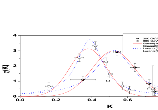
Figure 8: Inelasticity distributions $\chi(K=K_{q})$ (normalized to unity) obtained from [18] data for $\sqrt{s}=200$ GeV and $\sqrt{s}=900$ GeV (see text for details). $K_{q}$ is estimated from the $q$ and $\kappa_{q}$ parameters in Table 2 by using eq.(3). To guide the eyes obtained results were fitted by simple gaussian and lorentzian formulas ($\chi(K)\simeq\exp\left[-(K-\langle K\rangle)/(2a^{2})\right]$ and $\chi(K)\simeq\sigma/[4(K-\langle K\rangle)^{2}+\sigma^{2}]$, respectively, with $\sigma$ obtained for $K\in(0,1)$). Errors are estimated from the widths of the bins $\Delta N$ and the shapes and errors of $P(N)$ used in obtaining $\chi(K)$ [29].

It is interesting to notice that whereas data on rapidity distributions [14, 15, 16, 17] could be fitted both by the extensive (14) and nonextensive (19) distributions, similar data for rapidity distributions measured in restricted intervals of the multiplicity, $\Delta N$ [18], can be fitted only by means of the nonextensive $p_{q}(y)$ as given by eq.(19) [43]. The extensive approach with maximally correlated shapes and heights of distributions, as discussed above, is clearly too restrictive. Only relaxing this correlation by introducing parameter $q$ (i.e., by using nonextensive version of the information theory approach) allows for adequate fits to be performed, see Fig. 7 and Table 2. Notice that partial inelasticities of all kinds are clearly correlated with the multiplicity bins, the higher the multiplicity the bigger is the corresponding inelasticity. The same kind of correlations are observed at $200$ GeV between multiplicity and $q$, which increases with multiplicity. However, at $900$ GeV $q$ remains essentially constant. Following discussion in the previous paragraph one expects that it means an increase of the corresponding fluctuations. The question, however, remains, in which variable? We argue that the fluctuating variable in this case is inelasticity itself. The point is that particles filling a given interval of multiplicity $\Delta N$ can be produced in events with different, i.e., fluctuating values of $K$. As before, this fact would then lead to the apparent nonextensivity visualized by $q>1$ and measuring also the strength of such fluctuations represented by the variance,

$$\sigma^{2}(K)\,=\,\langle K\rangle^{2}(q-1).$$ (28)

However, in this case we do not have any independent estimation of $\sigma(K)$, therefore we could not exclude the action of some other, so far not yet disclosed, factors and propose the equivalent of eq. (27) for this case. On the other hand (28) could be used for estimation of the uncertainty in $K$ once its mean value and the nonextensivity parameter are known. For example, taking from Table 1 the corresponding values of $\langle K(s)\rangle$ and $q(s)$ one can estimate that $\langle K_{q}(200)\rangle=0.50\pm 0.23$ and $\langle K_{q}(900)\rangle=0.41\pm 0.22$.

The results for partial inelasticities obtained from fits shown in Fig. 7 allow us to calculate the corresponding inelasticities $K_{q}$ (by using (3)), cf. Table 2. These in turn, with the help of experimentally measured multiplicity distributions $P(n_{ch})$ (taken in this case from [44]) allow us to obtain, for the first time, the (normalized) inelasticity distribution $\chi(K=K_{q})$ presented in Fig. 8 [45]. This is one of the most important results which could be obtained only by using information theory approach in its nonextensive version. The gaussian and lorentzian fits shown here resemble very much the form of $\chi(K)$ obtained in the so called Interacting Gluon Model of high energy processes developed and studied in [11, 12, 10].

4 SUMMARY AND CONCLUSIONS

Using methods of information theory, both in its extensive and nonextensive versions, we have analysed $p\bar{p}$ collider data [14, 15, 16, 17, 18] and $pp$ fixed target data [31] on multiparticle production. Our investigation was aimed at the phenomenological, maximally model independent description, which would eventually result in estimations of inelasticities for these reactions, their energy dependence and, whenether possible, also in the inelasticity distributions $\chi(K)$. The information theory approach used by us leads to a comfortable situation where the only fitted parameter is either the inelasticity $K$ (when using extensive approach) or parameters $q$ and $\kappa_{q}$ (in its nonextensive counterpart) out of which one can reconstruct the inelasticity $K_{q}$ or $K_{q}^{(|y|\leq 4)}$. It turned out, that data for rapidity distributions obtained for the mean multiplicities can be fitted using both approaches. In this case the nonextensivity parameter $q$ obtained from fitting the rapidity distributions $dN/dy$ is practically identical to the parameter $q$, according to [23], responsible for dynamical fluctuations existing in hadronizing systems and showing up in the characteristic Negative Binomial form of the measured multiplicity distributions $P(N)$. This means therefore that in collider data for $p\bar{p}$ collisions and fixed target $pp$ data analysed in this way, there is no additional information to that used here. On the other hand rapidity distributions for fixed multiplicity intervals $\Delta N$ [18] can be described only by nonextensive approach and we argue that in this case $q$ reflects fluctuations in the inelasticity itself. These data were therefore used to estimate, for the first time at this energies ($200$ and $900$ GeV), the inelasticity distributions $\chi(K)$, cf. Fig. 8.

It is particularly interesting and worth of stressing here, that, formulas obtained by means of information theory are apparently identical with the corresponding equations of statistical models used to describe multiparticle production processes [32]. The point is, however, that - as was already stressed in appropriate cases before - the ”partition temperature” $T$ and the normalization $Z$ are in our case not free parameters anymore. The only freedom (in our case it was the choice of inelasticity $K$) is in providing the corresponding constraint equations, which should summarize our knowledge about the reaction under consideration. Once they are fixed, the other quantities (in particular $T$) follow. This constrains seriously such approach and therefore in cases where it fails one can either add new constraints or include some interactions by changing the very definition of how to measure the available information. The Tsallis entropy used here [22, 23, 27, 26, 35] is but only one example of what is possible, other definitions of information are also possible albeit not yet used in such circumstances [22, 46].

References

- [1] Yu.M.Shabelski, R.M.Weiner, G.Wilk and Z.Włodarczyk, J. Phys. G18 (1992) 1281 and references therein.
- [2] Cf. also: G.M.Frichter, T.K.Gaisser and T.Stanev, Phys. Rev. 56 (1997) 3135; A.A.Watson, Nucl. Phys. B (Proc. Suppl.) 60 (1998) 171; J.W.Cronin, ibid. 28 (1992) 213.
- [3] V.Kopenkin et al., Phys. Rev. D65 (2002) 072004.
- [4] J.Bellandi, R.Fleitas and J. Dias de Deus, J. Phys. G25 (1999) 1623; cf. also J.Bellandi, R.Fleitas and J. Dias de Deus and F.O.Durães, Eur. Phys. J. C11 (1999) 559.
- [5] For the most recent attempt to deduce inelasticity directly from the cosmic ray data provided by emulsion chambers see [6].
- [6] G.Wilk and Z.Włodarczyk, Phys. Rev. D59 (1999) 014025 and C.R.A.Augusto et al. Phys. Rev. D61 (2000) 012003.
- [7] T.Wibig, J.Phys. G27 (2001) 1633.
- [8] A.D.Erlykin and A.W.Wolfendale, How Should We Modify the High Energy Interaction Models?, hep-ph/0210129; to be published in Proc. of the XII ISVHECRI, CERN, Geneva, 15-19 July, 2002, Nucl. Phys. B Proc. Suppl. (2003).
- [9] R.Engel, Extensive Air Showers and Accelerator Data - The NEEDS Workshop, hep-ph/0212340, to be published in Proc. of the XII ISVHECRI, CERN, Geneva, 15-19 July, 2002, Nucl. Phys. B Proc. Suppl. (2003).
- [10] F.O.Durães, F.S.Navarra and G.Wilk, Phys. Rev. D58 (1998) 094034 and Leading particle and diffractive spectra in the Interacting Gluon Model, hep-ph/0209328, presented at Diffraction 2002, Alushta, Crimea (Ukraine), Aug. 31- Sept. 05, 2002, to be published in proceedings by Kluwer Acad. Pub. (2003).
- [11] G.N.Fowler, F.S.Navarra, M.Plümer, A.Vourdas, R.M.Weiner and G.Wilk, Phys. Lett. B214 (1988) 657 and Phys. Rev. C40 (1989) 1219; F.O. Durães, F.S. Navarra and G. Wilk, Phys. Rev. D47 (1993) 3049. Cf. also: Y.Hama and S.Paiva, Phys. Rev. Lett. 78 (1997) 3070 and S.Paiva, Y.Hama and T.Kodama, Phys. Rev. C55 (1997) 1455.
- [12] F.O.Durães, F.S.Navarra and G.Wilk, Phys. Rev. D50 (1994) 6804.
- [13] Y.-A.Chao, Nucl. Phys. B40 (1972) 475.
- [14] R.Baltrusaitis et al., Phys. Rev. Lett. 52(1993) 1380.
- [15] F.Abe et al., Phys. Rev. D41 (1990) 2330.
- [16] R.Harr et al. (P238 Collab.), Phys. Lett. B 401 (1997) 176.
- [17] E.Pare et al. (UA7 Collab.), Phys Lett. B 242 (1990) 531.
- [18] G.J.Alner et al. (UA5 Collab.), Z. Phys. C33 (1986) 1.
- [19] T.T.Chou and C.N.Yang, Phys. Rev. Lett. 54 (1985) 510 and Phys. Rev. D32 (1985) 1692.
- [20] J.Dias de Deus, Phys. Lett. B315 (1993) 188J or Bellandi et al. J. Phys. G23 (1997) 125 and references therein.
- [21] G.Wilk and Z.Włodarczyk, Phys. Rev. D43 (1991) 794.
- [22] C.Tsallis, in Nonextensive Statistical Mechanics and its Applications, S.Abe and Y.Okamoto (Eds.), Lecture Notes in Physics LPN560, Springer (2000).
- [23] G.Wilk and Z.Włodarczyk, Phys. Rev. Lett. 84 (2000) 2770; Chaos, Solitons and Fractals 13 (2002) 581 and Physica A305 (2002) 227.
- [24] One should mention here that there exists a formalism, which expresses both the Tsallis entropy (4) and the expectation values (6) using the so-called escort probability distributions [25]: . However, as was shown in [26], such an approach is different from the normal nonextensive formalism because the Tsallis entropy expressed in terms of the escort probability distributions has difficulty with the property of concavity. From our limited point of view, it seems that there is no problem in what concerns practical, phenomenological applications of nonextensivity as discussed in the present work. Namely, using one gets distributions of the type , which is, in fact, formally identical with that in (8), , provided we identify: , and . The mean value is now and (to be compared with ). Both distributions are identical and the problem, which of them better describes data is artificial. Therefore in what follows we shall use the approach leading to (8).
- [25] C.Tsallis, R.S.Mendes and A.R.Plastino, Physica A261 (1998) 534.
- [26] S.Abe, Phys. Lett. A275 (2000) 250.
- [27] C.Beck and E.G.D.Cohen, Superstatistics, cond-mat/0205097, to be published in Physica A (2003).
- [28] G.J.Alner et al., Phys. Lett. B167 (1986) 486.
- [29] C.Geich-Gimbel, Int. J. Mod. Phys. A4 (1989) 1527.
- [30] It could be argued that by allowing the growth of with we also include, at least to some extent, the growing with energy influence of hard collisions visualized as occurrence of the so called gluonic mini-jets, cf. [12].
- [31] C.De Marzo et al., Phys. Rev. D26 (1982) 1019 and D29 (1984) 2476.
- [32] Cf., for example, F.Becattini, Nucl. Phys. A702 (2002) 336 or F.Becattini and G.Passaleva, Eur. Phys. J. C23 (2002) 551 and references therein.
- [33] We shall not add here, as it is done in T.Osada, M.Maruyama and F.Takagi, Phys. Rev. D59, 014024 (1999), the charge conservation as the second possible constraint, but calculate our distribution for a given fixed total mean multiplicity .
- [34] A.Ohsawa, Prog. Theor. Phys. 92 (1994) 1005.
- [35] C.Beck, Physica A286 (200) 164.
- [36] R.Hagedorn, Nuovo Cim. Suppl. 3 (1965) 147; Nuovo Cim. A52 (1967) 64 and Riv. Nuovo Cim. 6 (1983) 1983.
- [37] F.S.Navarra, O.V.Utyuzh, G.Wilk and Z.Włodarczyk, Nuovo Cim. 24C (2001) 725.
- [38] G.Cocconi, Phys. Rev. 111 (1958) 1699.
- [39] M.Basile et al., Phys. Lett. B92 (1980) 367 and B95 (1980) 311.
- [40] M.Rybczyńsk, Z.Włodarczyk and G.Wilk, Rapidity spectra analysis in terms of nonextensive statistics approach, hep-ph/0206157, to be published in Proc. of the XII ISVHECRI, CERN, Geneva, 15-19 July, 2002, Nucl. Phys. B Proc. Suppl. (2003).
- [41] P.Carruthers and C.S.Shih, Int. J. Mod. Phys. A2 (1986) 1447.
- [42] For recent discussion of nonextensive statistics (using the escort probabilities approach [25, 24]) see C.E.Aguiar and T.Kodama, Nonextensive statistics and Multiplicity distributions in Hadronic Collisions, cond-matt/0207274, to be published in Physica A (2003).
- [43] Actually, only data on for and Gev will be used here because we have found that data for GeV (used previously in [19]), are incompatible with the corresponding data for the mean multiplicities .
- [44] R.E.Ansorge et al., Z. Phys. C43 (1989) 357.
- [45] Actually was also extracted before in D.Brick et al. Phys. Lett. B103 (1981) 242 but for much lower energy, GeV. Its shape was similar to what we have obtained and was fitted in G.N.Fowler et al., Phys. Lett. B145 (1984) 407 by a gamma function; cf. also results of [11].
- [46] Cf., for example, B.R.Frieden et al., Phys. Rev. E60 (1999) 48 and B.R.Frieden, Physics from Fisher information, Cambridge Univ. Press (1999).