CERN-TH/2003-011

hep-ph/0301256

A Closer Look at $B_{d,s}\to Df_{r}$ Decays and

Novel Avenues to Determine $\gamma$

Robert Fleischer

Theory Division, CERN, CH-1211 Geneva 23, Switzerland

Decays of neutral $B$ mesons originating from $b\to Dr$ $(r\in\{s,d\})$ processes, i.e. $B_{d}\to DK_{\rm S(L)}$, $B_{s}\to D\eta^{(^{\prime})},D\phi,...$ $(r=s)$ and $B_{s}\to DK_{\rm S(L)}$, $B_{d}\to D\pi^{0},D\rho^{0},...$ $(r=d)$ modes, offer valuable insights into CP violation. Here the neutral $D$ mesons may be observed through $D\to f_{\pm}$ or $D\to f_{\rm NE}$, where $f_{\pm}$ and $f_{\rm NE}$ are CP eigenstates and CP non-eigenstates, respectively. Recently, we pointed out that “untagged” and mixing-induced CP-violating $B_{d,s}\to D_{\pm}f_{s}$ observables provide a very efficient, theoretically clean determination of the angle $\gamma$ of the unitarity triangle. Here we perform a more detailed analysis of the $B_{d,s}\to D[\to f_{\pm}]f_{s}$ channels, and focus on $B_{d,s}\to D[\to f_{\rm NE}]f_{s}$, where interference effects between Cabibbo-favoured and doubly Cabibbo-suppressed $D$-meson decays lead to complications. We show that $\gamma$ can nevertheless be determined in an elegant and essentially unambiguous manner from the $B_{d,s}\to D[\to f_{\rm NE}]f_{s}$ observables with the help of the corresponding “untagged” $B_{d,s}\to D[\to f_{\pm}]f_{s}$ measurements. Moreover, we may also extract hadronic $B$- and $D$-decay parameters. Several interesting features of decays of the kind $B_{d,s}\to Df_{d}$ are also pointed out.

CERN-TH/2003-011
January 2003

1 Introduction

The exploration of CP violation, which was discovered in 1964 through the observation of $K_{\rm L}\to\pi^{+}\pi^{-}$ decays [1], is one of the hot topics in particle physics. In this decade, studies of $B$-meson decays will provide various stringent tests of the Kobayashi–Maskawa mechanism of CP violation [2], allowing us to accommodate this phenomenon in the Standard Model of electroweak interactions. At present, the experimental stage is governed by the asymmetric $e^{+}e^{-}$ $B$ factories operating at the $\Upsilon(4S)$ resonance, with their detectors BaBar (SLAC) and Belle (KEK). Interesting $B$-physics results are also soon expected from run II of the Tevatron [3]. Several strategies can only be fully exploited in the era of the LHC [4], in particular by LHCb (CERN) and BTeV (Fermilab).

Figure 1: Unitarity triangle of the CKM matrix.

The central target for the exploration of CP violation is the unitarity triangle of the Cabibbo–Kobayashi–Maskawa (CKM) matrix illustrated in Fig. 1, which can be determined through measurements of its sides on the one hand, and direct measurements of its angles through CP-violating effects in $B$ decays on the other hand (for a detailed review, see [5]). If we take into account next-to-leading order terms in the Wolfenstein expansion of the CKM matrix [6], following the prescription given in [7], we obtain the following coordinates for the apex of the unitarity triangle:

$$\overline{\rho}\equiv(1-\lambda^{2}/2)\rho,\quad\overline{\eta}\equiv(1-\lambda^{2}/2)\eta,$$ (1.1)

where $\lambda\equiv|V_{us}|=0.22$. The goal is to overconstrain the unitarity triangle as much as possible. In this respect, a first important milestone has already been achieved by the BaBar and Belle collaborations, who have announced the observation of CP violation in the $B$-meson system in the summer of 2001 [8]. This discovery was made possible by $B_{d}\to J/\psi K_{\rm S}$ and similar channels. As is well known, these modes allow us to determine $\sin\phi_{d}$, where $\phi_{d}$ denotes the CP-violating weak $B^{0}_{d}$–$\overline{B^{0}_{d}}$ mixing phase, which is given by $2\beta$ in the Standard Model. Using the present world average $\sin\phi_{d}=0.734\pm 0.054$ [9], we obtain the following twofold solution for $\phi_{d}$ itself:

$$\phi_{d}=\left(47^{+5}_{-4}\right)^{\circ}\,\lor\,\left(133^{+4}_{-5}\right)^{\circ},$$ (1.2)

where the former would be in perfect agreement with the “indirect” range implied by the CKM fits, $40^{\circ}\mathrel{\hbox{\hbox to0.0pt{\hbox{\lower 4.0pt\hbox{$\sim$}}\hss}\hbox{$<$}}}\phi_{d}\mathrel{\hbox{\hbox to0.0pt{\hbox{\lower 4.0pt\hbox{$\sim$}}\hss}\hbox{$<$}}}60^{\circ}$ [10], while the latter would correspond to new physics. The two solutions can be distinguished through a measurement of the sign of $\cos\phi_{d}$. Several strategies to accomplish this important task were proposed [11]. For example, in the $B\to J/\psi K$ system, $\mbox{sgn}(\cos\phi_{d})$ can be extracted with the help of the time-dependent angular distribution of the $B_{d}\to J/\psi[\to\ell^{+}\ell^{-}]K^{\ast}[\to\pi^{0}K_{\rm S}]$ decay products if the sign of a hadronic parameter $\cos\delta_{f}$, involving a strong phase $\delta_{f}$, is fixed through factorization [12, 13]. This analysis is already in progress at the $B$ factories [14]. A remarkable link between the two solutions for $\phi_{d}$ and ranges for $\gamma$ is also suggested by recent data on the CP-violating $B_{d}\to\pi^{+}\pi^{-}$ observables [15].

Interesting tools for the exploration of CP violation are provided by $B_{d}\to DK_{\rm S(L)}$, $B_{s}\to D\eta^{(^{\prime})},D\phi,...$ and $B_{s}\to DK_{\rm S(L)}$, $B_{d}\to D\pi^{0},D\rho^{0},...$ modes, which originate from $b\to Ds$ and $b\to Dd$ transitions, respectively, and receive only contributions from tree-diagram-like topologies [16]–[18]. The neutral $D$ mesons may be observed through decays into CP eigenstates $f_{\pm}$, or through decays into CP non-eigenstates $f_{\rm NE}$. In a recent paper [19], we pointed out that $B_{d}\to D_{\pm}K_{\rm S(L)}$ and $B_{s}\to D_{\pm}\eta^{(^{\prime})},D_{\pm}\phi,...$ decays, where $D_{+}$ and $D_{-}$ denote the CP-even and CP-odd eigenstates of the neutral $D$-meson system, respectively, offer very efficient, theoretically clean determinations of the angle $\gamma$ of the unitarity triangle. In this strategy, only “untagged” and mixing-induced CP-violating observables are employed, which satisfy a very simple relation, allowing us to determine $\tan\gamma$. Using a plausible dynamical assumption, $\gamma$ can be fixed in an essentially unambiguous manner. The corresponding formalism can also be applied to $B_{d}\to D_{\pm}\pi^{0},D_{\pm}\rho^{0},...$ and $B_{s}\to D_{\pm}K_{\rm S(L)}$ decays. Although these modes appear less attractive for the extraction of $\gamma$, they provide interesting determinations of $\sin\phi_{q}$. In comparison with the conventional $B_{d}\to J/\psi K_{\rm S(L)}$ and $B_{s}\to J/\psi\phi$ methods, these extractions do not suffer from any penguin uncertainties, and are theoretically cleaner by one order of magnitude.

In the present paper, we give a more detailed discussion of the $D_{\pm}$ case by having a closer look at $D\to f_{\pm}$ processes, and focus on the CP non-eigenstate $D\to f_{\rm NE}$ case. Here we have to deal with interference effects between Cabibbo-favoured and doubly Cabibbo-suppressed $D$-meson decays, which lead to certain complications [17, 20]. We point out that $\gamma$ can nevertheless be determined in a powerful and essentially unambiguous way from the time-dependent $B_{d}\to D[\to f_{\rm NE}]K_{\rm S(L)}$, $B_{s}\to D[\to f_{\rm NE}]\eta^{(^{\prime})},D[\to f_{\rm NE}]\phi,...$ rates with the help of simple “untagged” measurements of the corresponding $B_{d}\to D_{\pm}K_{\rm S(L)}$, $B_{s}\to D_{\pm}\eta^{(^{\prime})},D_{\pm}\phi,...$ processes. Moreover, we may also extract interesting hadronic $B$- and $D$-decay parameters. This strategy can be implemented with the help of transparent formulae in an analytical manner. Decays of the kind $B_{s}\to DK_{\rm S(L)}$, $B_{d}\to D\pi^{0},D\rho^{0},...$ also exhibit interesting features, but they appear not to be as attractive for the extraction of $\gamma$ as their $b\to Ds$ counterparts, since they have a different CKM structure.

For the testing of the Kobayashi–Maskawa mechanism of CP violation [2], it is essential to measure $\gamma$ in a variety of ways. In particular, it will be very interesting to compare the theoretically clean values for $\gamma$ obtained with the help of the new strategies proposed here with the results that will be provided by other approaches. In this context, $B\to\pi K$ and $B_{s}\to K^{+}K^{-}$, $B_{d}\to\pi^{+}\pi^{-}$ modes are important examples, allowing the extraction of $\gamma$ through $SU(3)$ flavour-symmetry arguments (for overviews, see [21]). Several theoretically clean strategies were also proposed, employing various different pure tree-diagram-like $B$ decays (see, for instance, [20] and [22]–[30]). In general, these approaches are either conceptually simple but experimentally very challenging, or do not allow transparent extractions of $\gamma$ through simple analytical expressions, thereby also complicating things considerably and yielding multiple discrete ambiguities. Alternative approaches to extract weak phases from neutral $b\to Ds$ modes can be found in [16]–[18].

The outline of this paper is as follows: in Section 2, we introduce a convenient notation and discuss the time evolution and amplitude structure of neutral $B$-meson decays caused by $b\to Ds$ and $b\to Dd$ transitions. In Section 3, we then turn to the case where the neutral $D$ mesons are observed through decays into CP eigenstates $f_{\pm}$, whereas we shall focus on the interesting opposite case, where the $D$ mesons are observed through decays into CP non-eigenstates $f_{\rm NE}$, in Section 4. The main approach of this paper is presented in Section 5, and is also illustrated there with the help of a few instructive examples. Finally, we conclude in Section 6.

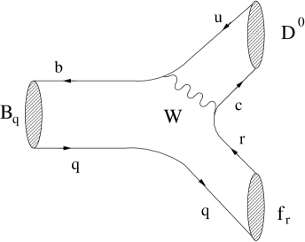
Figure 2: Feynman diagrams contributing to $B_{q}^{0}\to D^{0}f_{r}$ and $\overline{B_{q}^{0}}\to D^{0}\overline{f_{r}}$.

2 Notation, Time Evolution and Decay Amplitudes

2.1 Notation

The decays we shall consider in the following analysis may be written generically as $B^{0}_{q}\to D^{0}f_{r}$, $\overline{B^{0}_{q}}\to D^{0}\overline{f_{r}}$, where $q\in\{d,s\}$ and $r\in\{d,s\}$, as can be seen in Fig. 2. Note that the $q$ quark is contained in $f_{r}$; in order not to complicate the notation unnecessarily, we do not indicate this explicitly through another label $q$ that should, in principle, be added to $f_{r}$. If we require that $f_{r}$ be a CP-self-conjugate state, i.e. satisfies

$$({\cal CP})|f_{r}\rangle=\eta_{\rm CP}^{f_{r}}|f_{r}\rangle,$$ (2.1)

$B^{0}_{q}$ and $\overline{B^{0}_{q}}$ may both decay into the same state $D^{0}f_{r}$, thereby leading to interference effects between $B^{0}_{q}$–$\overline{B^{0}_{q}}$ mixing and decay processes. Let us illustrate this abstract but quite efficient notation by giving a few examples:

• $r=s$:   $B_{d}\to DK_{\rm S(L)}$ $(q=d)$;   $B_{s}\to D\eta^{(^{\prime})},D\phi,...$ $(q=s)$.

• $r=d$:   $B_{s}\to DK_{\rm S(L)}$ $(q=s)$;   $B_{d}\to D\pi^{0},D\rho^{0},...$ $(q=d)$.

All these decays are governed by the colour-suppressed tree-diagram-like topologies shown in Fig. 2. In the case of $r=q$, also exchange topologies may contribute. However, these contributions do not modify the phase structure of the corresponding decay amplitudes discussed in Subsection 2.3, since they enter with the same CKM factors as the colour-suppressed tree topologies. The $\overline{B^{0}_{d}}\to D^{0}\pi^{0}$ mode has already been observed by the Belle, CLEO and BaBar collaborations, with branching ratios at the $3\times 10^{-4}$ level [31]. Interestingly, also the observation of the $\overline{B^{0}_{d}}\to D^{0}\overline{K^{0}}$ channel was very recently announced by the Belle collaboration [32], measuring the branching ratio $(5.0^{+1.3}_{-1.2}\pm 0.6)\times 10^{-5}$.

2.2 Time Evolution

If both a $B^{0}_{q}$ and a $\overline{B^{0}_{q}}$ meson may decay into the same final state $f$, as is the case for the modes specified above, we obtain the following time-dependent rate asymmetry [5]:

$$\frac{\Gamma(B^{0}_{q}(t)\to f)-\Gamma(\overline{B^{0}_{q}}(t)\to f)}{\Gamma(B^{0}_{q}(t)\to f)+\Gamma(\overline{B^{0}_{q}}(t)\to f)}$$ (2.2)

$$=\left[\frac{C(B_{q}\to f)\cos(\Delta M_{q}t)+S(B_{q}\to f)\sin(\Delta M_{q}t)}{\cosh(\Delta\Gamma_{q}t/2)-{\cal A}_{\rm\Delta\Gamma}(B_{q}\to f)\sinh(\Delta\Gamma_{q}t/2)}\right],$$

where $\Gamma(B^{0}_{q}(t)\to f)$ and $\Gamma(\overline{B^{0}_{q}}(t)\to f)$ denote the time-dependent decay rates for initially, i.e. at time $t=0$, present $B^{0}_{q}$ and $\overline{B^{0}_{q}}$ states, and $\Delta M_{q}\equiv M_{\rm H}^{(q)}-M_{\rm L}^{(q)}>0$ and $\Delta\Gamma_{q}\equiv\Gamma_{\rm H}^{(q)}-\Gamma_{\rm L}^{(q)}$ are the mass and decay width differences of the $B_{q}$ mass eigenstates, respectively. The observables $C(B_{q}\to f)$ and $S(B_{q}\to f)$ are given by

$$C(B_{q}\to f)=\frac{1-\bigl{|}\xi_{f}^{(q)}\bigr{|}^{2}}{1+\bigl{|}\xi_{f}^{(q)}\bigr{|}^{2}}\quad\mbox{and}\quad S(B_{q}\to f)=\frac{2\,\mbox{Im}\,\xi^{(q)}_{f}}{1+\bigl{|}\xi^{(q)}_{f}\bigr{|}^{2}},$$ (2.3)

respectively, where

$$\xi_{f}^{(q)}=e^{-i\Theta_{{M}_{12}}^{(q)}}\frac{A(\overline{B_{q}^{0}}\to f)}{A(B_{q}^{0}\to f)}$$ (2.4)

measures the strength of the interference effects between the $B^{0}_{q}$–$\overline{B^{0}_{q}}$ mixing and decay processes. Here

$$\Theta_{{M}_{12}}^{(q)}-\pi+\phi_{\rm CP}(B_{q})=2\,\mbox{arg}(V_{tq}^{\ast}V_{tb})\equiv\phi_{q}\stackrel{{\scriptstyle\rm SM}}{{=}}\left\{\begin{array}[]{cl}+2\beta={\cal O}(50^{\circ})&~{}~{}\mbox{($q=d$)}\\ -2\lambda^{2}\eta={\cal O}(-2^{\circ})&~{}~{}\mbox{($q=s$)}\end{array}\right.$$ (2.5)

is the CP-violating weak $B^{0}_{q}$–$\overline{B^{0}_{q}}$ mixing phase, which is – within the Standard Model – negligibly small in the $B_{s}$-meson system; the convention-dependent phase $\phi_{\rm CP}(B_{q})$ is defined through

$$({\cal CP})|B^{0}_{q}\rangle=e^{i\phi_{\rm CP}(B_{q})}|\overline{B^{0}_{q}}\rangle,\quad({\cal CP})|\overline{B^{0}_{q}}\rangle=e^{-i\phi_{\rm CP}(B_{q})}|B^{0}_{q}\rangle.$$ (2.6)

As we will see below, $\phi_{\rm CP}(B_{q})$ is cancelled through the amplitude ratio in (2.4). The width difference $\Delta\Gamma_{q}$ provides another observable,

$${\cal A}_{\rm\Delta\Gamma}(B_{q}\to f)=\frac{2\,\mbox{Re}\,\xi^{(q)}_{f}}{1+\bigl{|}\xi^{(q)}_{f}\bigr{|}^{2}},$$ (2.7)

which is, however, not independent from $C(B_{q}\to f)$ and $S(B_{q}\to f)$, satisfying

$$\Bigl{[}C(B_{q}\to f)\Bigr{]}^{2}+\Bigl{[}S(B_{q}\to f)\Bigr{]}^{2}+\Bigl{[}{\cal A}_{\Delta\Gamma}(B_{q}\to f)\Bigr{]}^{2}=1.$$ (2.8)

This observable could be determined from the “untagged” rate

$$\langle\Gamma(B_{q}(t)\to f)\rangle \equiv \Gamma(B^{0}_{q}(t)\to f)+\Gamma(\overline{B^{0}_{q}}(t)\to f)=\left[\Gamma(B^{0}_{q}\to f)+\Gamma(\overline{B^{0}_{q}}\to f)\right]$$ (2.9)

$$\times\left[\cosh(\Delta\Gamma_{q}t/2)-{\cal A}_{\rm\Delta\Gamma}(B_{q}\to f)\,\sinh(\Delta\Gamma_{q}t/2)\right]e^{-\Gamma_{q}t},$$

where the oscillatory $\cos(\Delta M_{q}t)$ and $\sin(\Delta M_{q}t)$ terms cancel, and $\Gamma_{q}\equiv(\Gamma_{\rm H}^{(q)}+\Gamma_{\rm L}^{(q)})/2$ denotes the average decay width [33]. However, in the case of the $B_{d}$-meson system, the width difference is negligibly small, so that the time evolution of (2.9) is essentially given by the well-known exponential $e^{-\Gamma_{d}t}$. On the other hand, the width difference $\Delta\Gamma_{s}$ of the $B_{s}$-meson system may be as large as ${\cal O}(-10\%)$ (for a recent review, see [34]).

In the discussion given below, we shall see – as in [19] – that observables provided by the untagged rates specified in (2.9) are a key element for an efficient determination of $\gamma$ from $B_{q}\to Df_{s}$ modes. In contrast to the strategies proposed in [33, 35], we do not have to rely on a sizeable width difference $\Delta\Gamma_{q}$; the untagged measurements are only required to extract the “unevolved”, i.e. time-independent, untagged rates

$$\langle\Gamma(B_{q}\to f)\rangle\equiv\Gamma(B^{0}_{q}\to f)+\Gamma(\overline{B^{0}_{q}}\to f).$$ (2.10)

Consequently, we will not discuss the effects that may be caused by a possible sizeable value of $\Delta\Gamma_{s}$ in further detail. They could be taken into account straightforwardly.

Concerning the time evolution of the $B_{q}\to Df_{r}$ modes analysed in this paper, the subsequent decay of the neutral $D$-meson state plays a crucial rôle. Let us assume that this decay, $D\to f_{D}$, occurs at time $t=t^{\prime}$ after the decay of the $B_{q}$ meson into $Df_{r}$. In this case, we have to consider decay amplitudes of the kind

$$A(B^{0}_{q}(t)\to D(t^{\prime})[\to f_{D}]f_{r}),$$ (2.11)

and have in principle to deal with $D^{0}$–$\overline{D^{0}}$ mixing for $t^{\prime}>0$. However, within the Standard Model, this phenomenon is very small. Neglecting hence the mixing effects, the time evolution of the neutral $|D\rangle$ states is given by

$$|D^{0}(t^{\prime})\rangle=e^{-iM_{D}t^{\prime}}e^{-\Gamma_{D}t^{\prime}/2}|D^{0}\rangle,\quad|\overline{D^{0}}(t^{\prime})\rangle=e^{-iM_{D}t^{\prime}}e^{-\Gamma_{D}t^{\prime}/2}|\overline{D^{0}}\rangle,$$ (2.12)

so that (2.11) yields a time-dependent rate of the following simple structure:

$$\Gamma(B^{0}_{q}(t)\to D(t^{\prime})[\to f_{D}]f_{r})=e^{-\Gamma_{D}t^{\prime}}\Gamma(B^{0}_{q}(t)\to D[\to f_{D}]f_{r}),$$ (2.13)

where $\Gamma(B^{0}_{q}(t)\to D[\to f_{D}]f_{r})$ corresponds to the rates entering (2.2), and $\Gamma_{D}$ denotes the decay width of the neutral $D$ mesons. As is well known, $D^{0}$–$\overline{D^{0}}$ mixing may be enhanced through new physics. Should this actually be the case, the mixing effects could be included through a measurement of the $D^{0}$–$\overline{D^{0}}$ mixing parameters [36]. Note that $D^{0}$–$\overline{D^{0}}$ mixing does not lead to any effects in the case of $t^{\prime}=0$, even if this phenomenon should be made sizeable by the presence of new physics. In the following considerations, we shall neglect $D^{0}$–$\overline{D^{0}}$ mixing for simplicity. Moreover, we shall assume that CP violation in $D$ decays is also negligible, as in the Standard Model. In analogy to $D^{0}$–$\overline{D^{0}}$ mixing, these effects could also be enhanced through new physics. In the following sections, we will therefore emphasize clearly whenever this assumption enters.

Note that also the tiny “indirect” CP violation in the neutral kaon system has – at least in principle – to be taken into account if $K_{\rm S}$ or $K_{\rm L}$ states are involved. This could be done through the corresponding experimental $K$-decay data. However, it appears very unlikely that the experimental accuracy of the strategies for the determination of $\gamma$ discussed below will ever reach a level where these effects may play any rôle from a practical point of view.

2.3 Decay Amplitudes

In order to analyse the structure of the $B_{q}\to Df_{r}$ decay amplitudes, we employ appropriate low-energy effective Hamiltonians [5]:

$${\cal H}_{\rm eff}(\overline{B^{0}_{q}}\to D^{0}f_{r}) = \frac{G_{\rm F}}{\sqrt{2}}\,\overline{v}_{r}\left[\overline{{\cal O}}_{1}^{\,r}\,{C}_{1}(\mu)+\overline{{\cal O}}_{2}^{\,r}\,{C}_{2}(\mu)\right]$$ (2.14)

$${\cal H}_{\mbox{{\scriptsize eff}}}(B^{0}_{q}\to D^{0}f_{r}) = \frac{G_{\rm F}}{\sqrt{2}}\,v_{r}^{\ast}\left[{\cal O}_{1}^{r\dagger}\,{C}_{1}(\mu)+{\cal O}_{2}^{r\dagger}\,{C}_{2}(\mu)\right],$$ (2.15)

where $\overline{{\cal O}}_{k}^{\,r}$ and ${\cal O}_{k}^{\,r}$ denote current–current operators, which are given by

$$\begin{array}[]{rclrcl}\overline{{\cal O}}_{1}^{\,r}&=&(\overline{r}_{\alpha}u_{\beta})_{\mbox{{\scriptsize V--A}}}\left(\overline{c}_{\beta}b_{\alpha}\right)_{\mbox{{\scriptsize V--A}}},&~{}~{}\overline{{\cal O}}_{2}^{\,r}&=&(\overline{r}_{\alpha}u_{\alpha})_{\mbox{{\scriptsize V--A}}}\left(\overline{c}_{\beta}b_{\beta}\right)_{\mbox{{\scriptsize V--A}}},\\ &&&&&\\ {\cal O}_{1}^{\,r}&=&(\overline{r}_{\alpha}c_{\beta})_{\mbox{{\scriptsize V--A}}}\left(\overline{u}_{\beta}b_{\alpha}\right)_{\mbox{{\scriptsize V--A}}},&~{}~{}{\cal O}_{2}^{\,r}&=&(\overline{r}_{\alpha}c_{\alpha})_{\mbox{{\scriptsize V--A}}}\left(\overline{u}_{\beta}b_{\beta}\right)_{\mbox{{\scriptsize V--A}}},\end{array}$$ (2.16)

and

$$v_{s}=V_{cs}^{\ast}V_{ub}=A\lambda^{3}R_{b}e^{-i\gamma},\quad\overline{v}_{s}=V_{us}^{\ast}V_{cb}=A\lambda^{3},$$ (2.17)

$$v_{d}=V_{cd}^{\ast}V_{ub}=-\left(\frac{A\lambda^{4}R_{b}}{1-\lambda^{2}/2}\right)e^{-i\gamma},\quad\overline{v}_{d}=V_{ud}^{\ast}V_{cb}=A\lambda^{2}(1-\lambda^{2}/2)$$ (2.18)

are CKM factors, with (for the numerical values, see [37])

$$A\equiv\frac{1}{\lambda^{2}}|V_{cb}|=0.83\pm 0.02,$$ (2.19)

$$R_{b}\equiv\left(1-\frac{\lambda^{2}}{2}\right)\frac{1}{\lambda}\left|\frac{V_{ub}}{V_{cb}}\right|=\sqrt{\overline{\rho}^{2}+\overline{\eta}^{2}}=0.39\pm 0.04.$$ (2.20)

Using (2.14), we may write

$$A(\overline{B^{0}_{q}}\to D^{0}f_{r})=\langle f_{r}D^{0}|{\cal H}_{\rm eff}(\overline{B^{0}_{q}}\to D^{0}f_{r})|\overline{B^{0}_{q}}\rangle=\frac{G_{\rm F}}{\sqrt{2}}\overline{v}_{r}\overline{M}_{f_{r}},$$ (2.21)

where

$$\overline{M}_{f_{r}}\equiv\langle f_{r}D^{0}|\overline{{\cal O}}_{1}^{\,r}\,{C}_{1}(\mu)+\overline{{\cal O}}_{2}^{\,r}\,{C}_{2}(\mu)|\overline{B^{0}_{q}}\rangle.$$ (2.22)

On the other hand, we have

$$A(B^{0}_{q}\to D^{0}f_{r})=\langle f_{r}D^{0}|{\cal H}_{\rm eff}(B^{0}_{q}\to D^{0}f_{r})|B^{0}_{q}\rangle,$$ (2.23)

which we may rewrite as

$$A(B^{0}_{q}\to D^{0}f_{r}) = \langle f_{r}D^{0}|({\cal CP})^{\dagger}({\cal CP}){\cal H}_{\rm eff}(B^{0}_{q}\to D^{0}f_{r})({\cal CP})^{\dagger}({\cal CP})|B^{0}_{q}\rangle$$ (2.24)

$$= (-1)^{L}\eta_{\rm CP}^{f_{r}}e^{i[\phi_{\rm CP}(B_{q})-\phi_{\rm CP}(D)]}\frac{G_{\rm F}}{\sqrt{2}}\,v_{r}^{\ast}M_{f_{r}},$$

where

$$M_{f_{r}}\equiv\langle f_{r}\overline{D^{0}}|{\cal O}_{1}^{\,r}\,{C}_{1}(\mu)+{\cal O}_{2}^{\,r}\,{C}_{2}(\mu)|\overline{B^{0}_{q}}\rangle.$$ (2.25)

Here we have employed

$$({\cal CP})^{\dagger}({\cal CP})=\hat{1},$$ (2.26)

$$({\cal CP}){\cal O}_{k}^{\,r\dagger}({\cal CP})^{\dagger}={\cal O}_{k}^{\,r},$$ (2.27)

as well as

$$({\cal CP})|D^{0}f_{r}\rangle=(-1)^{L}\eta_{\rm CP}^{f_{r}}e^{i\phi_{\rm CP}(D)}|\overline{D^{0}}f_{r}\rangle,$$ (2.28)

where $L$ denotes the angular momentum of the $D^{0}f_{r}$ state, and

$$({\cal CP})|D^{0}\rangle=e^{i\phi_{\rm CP}(D)}|\overline{D^{0}}\rangle,\quad({\cal CP})|\overline{D^{0}}\rangle=e^{-i\phi_{\rm CP}(D)}|D^{0}\rangle,$$ (2.29)

in analogy to (2.6). In the following, we shall use the abbreviation

$$\eta_{f_{r}}\equiv(-1)^{L}\eta_{\rm CP}^{f_{r}}.$$ (2.30)

For convenience, we have collected in Table 1 the values of $L$, $\eta_{\rm CP}^{f_{r}}$ and $\eta_{f_{r}}$ for various decay channels of the kind specified in Subsection 2.1.

$r=s$	$r=d$	$L$	$\eta_{\rm CP}^{f_{r}}$	$\eta_{f_{r}}$
$\overline{B^{0}_{d}}\to D^{0}K_{\rm S(L)}$	$\overline{B^{0}_{s}}\to D^{0}K_{\rm S(L)}$	0	$+1(-1)$	$+1(-1)$
$\overline{B^{0}_{s}}\to D^{0}\eta^{(^{\prime})}$	$\overline{B^{0}_{d}}\to D^{0}\pi^{0}$	0	$-1$	$-1$
$\overline{B^{0}_{s}}\to D^{0}\phi$	$\overline{B^{0}_{d}}\to D^{0}\rho^{0}$	1	$+1$	$-1$

Table 1: The values of $L$, $\eta_{\rm CP}^{f_{r}}$ and $\eta_{f_{r}}$ for various $\overline{B_{q}^{0}}\to D^{0}f_{r}$ modes.

Let us now consider the decays $\overline{B^{0}_{q}}\to\overline{D^{0}}f_{r}$ and $B^{0}_{q}\to\overline{D^{0}}f_{r}$, which are described by

$${\cal H}_{\mbox{{\scriptsize eff}}}(\overline{B^{0}_{q}}\to\overline{D^{0}}f_{r}) = \frac{G_{\rm F}}{\sqrt{2}}\,v_{r}\left[{\cal O}_{1}^{r}\,{C}_{1}(\mu)+{\cal O}_{2}^{r}\,{C}_{2}(\mu)\right]$$ (2.31)

$${\cal H}_{\rm eff}(B^{0}_{q}\to\overline{D^{0}}f_{r}) = \frac{G_{\rm F}}{\sqrt{2}}\,\overline{v}_{r}^{\ast}\left[\overline{{\cal O}}_{1}^{\,r\dagger}\,{C}_{1}(\mu)+\overline{{\cal O}}_{2}^{\,r\dagger}\,{C}_{2}(\mu)\right],$$ (2.32)

yielding the following transition amplitudes:

$$A(\overline{B^{0}_{q}}\to\overline{D^{0}}f_{r})=\frac{G_{\rm F}}{\sqrt{2}}v_{r}M_{f_{r}}$$ (2.33)

$$A(B^{0}_{q}\to\overline{D^{0}}f_{r})=\eta_{f_{r}}e^{i[\phi_{\rm CP}(B_{q})+\phi_{\rm CP}(D)]}\frac{G_{\rm F}}{\sqrt{2}}\overline{v}_{r}^{\ast}\overline{M}_{f_{r}}.$$ (2.34)

For the time-dependent decay rates, the following amplitude ratios play a key rôle:

$$\frac{A(\overline{B^{0}_{q}}\to D^{0}f_{r})}{A(B^{0}_{q}\to D^{0}f_{r})}=\eta_{f_{r}}e^{-i\phi_{\rm CP}(B_{q})}\frac{\overline{v}_{r}}{v_{r}^{\ast}}\frac{1}{a_{f_{r}}e^{i\delta_{f_{r}}}}$$ (2.35)

$$\frac{A(\overline{B^{0}_{q}}\to\overline{D^{0}}f_{r})}{A(B^{0}_{q}\to\overline{D^{0}}f_{r})}=\eta_{f_{r}}e^{-i\phi_{\rm CP}(B_{q})}\frac{v_{r}}{\overline{v}_{r}^{\ast}}a_{f_{r}}e^{i\delta_{f_{r}}},$$ (2.36)

where

$$a_{f_{r}}e^{i\delta_{f_{r}}}\equiv e^{-i\phi_{\rm CP}(D)}\frac{M_{f_{r}}}{\overline{M}_{f_{r}}}=e^{-i\phi_{\rm CP}(D)}\left[\frac{\langle f_{r}\overline{D^{0}}|{\cal O}_{1}^{\,r}\,{C}_{1}(\mu)+{\cal O}_{2}^{\,r}\,{C}_{2}(\mu)|\overline{B^{0}_{q}}\rangle}{\langle f_{r}D^{0}|\overline{{\cal O}}_{1}^{\,r}\,{C}_{1}(\mu)+\overline{{\cal O}}_{2}^{\,r}\,{C}_{2}(\mu)|\overline{B^{0}_{q}}\rangle}\right].$$ (2.37)

Let us illustrate the calculation of the hadronic parameter $a_{f_{r}}e^{i\delta_{f_{r}}}$ using the factorization approach, which yields

$$\left.\langle f_{r}\overline{D^{0}}|{\cal O}_{1}^{\,r}\,{C}_{1}(\mu)+{\cal O}_{2}^{\,r}\,{C}_{2}(\mu)|\overline{B^{0}_{q}}\rangle\right|_{\rm fact}=a_{2}\langle\overline{D^{0}}|(\overline{u}_{\beta}c_{\beta})_{\mbox{{\scriptsize V--A}}}|0\rangle\langle f_{r}|(\overline{r}_{\alpha}b_{\alpha})_{\mbox{{\scriptsize V--A}}}|\overline{B^{0}_{q}}\rangle$$

$$=-e^{i\phi_{\rm CP}(D)}a_{2}\langle D^{0}|(\overline{c}_{\beta}u_{\beta})_{\mbox{{\scriptsize V--A}}}|0\rangle\langle f_{r}|(\overline{r}_{\alpha}b_{\alpha})_{\mbox{{\scriptsize V--A}}}|\overline{B^{0}_{q}}\rangle$$ (2.38)

and

$$\left.\langle f_{r}D^{0}|\overline{{\cal O}}_{1}^{\,r}\,{C}_{1}(\mu)+\overline{{\cal O}}_{2}^{\,r}\,{C}_{2}(\mu)|\overline{B^{0}_{q}}\rangle\right|_{\rm fact}=a_{2}\langle D^{0}|(\overline{c}_{\beta}u_{\beta})_{\mbox{{\scriptsize V--A}}}|0\rangle\langle f_{r}|(\overline{r}_{\alpha}b_{\alpha})_{\mbox{{\scriptsize V--A}}}|\overline{B^{0}_{q}}\rangle,$$ (2.39)

where

$$a_{2}=C_{1}(\mu_{\rm F})+\frac{C_{2}(\mu_{\rm F})}{N_{\rm C}}$$ (2.40)

is the well-known colour-suppression factor, with a factorization scale $\mu_{\rm F}$ and a number $N_{\rm C}$ of quark colours. Inserting (2.38) and (2.39) into (2.37), we observe that the convention-dependent phase $\phi_{\rm CP}(D)$ cancels – as it has to – and eventually arrive at the simple result

$$\left.a_{f_{r}}e^{i\delta_{f_{r}}}\right|_{\rm fact}=-1,$$ (2.41)

where the factorized hadronic matrix elements cancel as well. In particular, we conclude that $\left.\delta_{f_{r}}\right|_{\rm fact}=180^{\circ}$. Here it pays off to have kept the convention-dependent phase $\phi_{\rm CP}(D)$ explicitly in our calculation. If we look at the Feynman diagrams shown in Fig. 2 and contract the propagators of the $W$ bosons, we observe that the hadronic matrix elements entering (2.37) are related to each other through an interchange of all up and charm quarks and are hence very similar. Since $a_{f_{r}}e^{i\delta_{f_{r}}}$ is governed by the ratio of these matrix elements, and $\delta_{f_{r}}$ measures the relative strong phase between them, we expect $\delta_{f_{r}}$ to differ moderatly from the trivial value of $180^{\circ}$, even if the hadronic matrix elements themselves may deviate sizeably from the factorization case, as advocated in [38] (note that the recently developed QCD factorization approach [39] does not apply to $B_{q}\to Df_{r}$ modes). In particular, the assumption

$$\cos\delta_{f_{r}}<0,$$ (2.42)

which is satisfied for the whole range of $90^{\circ}<\delta_{f_{r}}<270^{\circ}$, is very plausible.

For the following considerations, it is convenient to rewrite (2.35) and (2.36) with the help of (2.17) and (2.18) as follows:

$$\frac{A(\overline{B^{0}_{q}}\to D^{0}f_{r})}{A(B^{0}_{q}\to D^{0}f_{r})}=\eta_{f_{r}}e^{-i\phi_{\rm CP}(B_{q})}e^{-i\gamma}\frac{1}{x_{f_{r}}e^{i\delta_{f_{r}}}}$$ (2.43)

$$\frac{A(\overline{B^{0}_{q}}\to\overline{D^{0}}f_{r})}{A(B^{0}_{q}\to\overline{D^{0}}f_{r})}=\eta_{f_{r}}e^{-i\phi_{\rm CP}(B_{q})}e^{-i\gamma}x_{f_{r}}e^{i\delta_{f_{r}}},$$ (2.44)

where

$$x_{f_{s}}\equiv R_{b}a_{f_{s}},\quad x_{f_{d}}\equiv-\left(\frac{\lambda^{2}R_{b}}{1-\lambda^{2}}\right)a_{f_{d}}.$$ (2.45)

Note that

$$\frac{x_{f_{d}}}{x_{f_{s}}}\approx-\left(\frac{\lambda^{2}}{1-\lambda^{2}}\right)=-0.05$$ (2.46)

reflects that the interference effects between the $\overline{B^{0}_{q}}\to\overline{D^{0}}f_{d}$ and $B^{0}_{q}\to\overline{D^{0}}f_{d}$ decay paths are doubly Cabibbo-suppressed, in contrast to the favourable situation in $\overline{B^{0}_{q}}\to\overline{D^{0}}f_{s}$ and $B^{0}_{q}\to\overline{D^{0}}f_{s}$, showing large interference effects of order $R_{b}\approx 0.4$.

3 Case of $B_{q}\to D[\to f_{\pm}]f_{r}$

3.1 Amplitudes

Let us now apply the formulae derived in the previous section to analyse the case where the neutral $D$ mesons are observed through their decays into CP eigenstates $f_{+}$ and $f_{-}$ with eigenvalues $+1$ and $-1$, respectively. Important examples are $f_{+}=K^{+}K^{-},\pi^{+}\pi^{-}$ and $f_{-}=K_{\rm S}\pi^{0},K_{\rm S}\phi$. The $\overline{B^{0}_{q}}\to D[\to f_{\pm}]f_{r}$ amplitude is given by

$$A(\overline{B^{0}_{q}}\to D[\to f_{\pm}]f_{r})=A(\overline{B^{0}_{q}}\to D^{0}f_{r})A(D^{0}\to f_{\pm})+A(\overline{B^{0}_{q}}\to\overline{D^{0}}f_{r})A(\overline{D^{0}}\to f_{\pm})$$

$$=\frac{G_{\rm F}}{\sqrt{2}}\overline{v}_{r}\overline{M}_{f_{r}}A(D^{0}\to f_{\pm})\left[1+\frac{v_{r}}{\overline{v}_{r}}\frac{M_{f_{r}}}{\overline{M}_{f_{r}}}\frac{A(\overline{D^{0}}\to f_{\pm})}{A(D^{0}\to f_{\pm})}\right].$$ (3.1)

If we neglect CP-violating effects in neutral $D$-meson decays, i.e. assume that the corresponding low-energy effective Hamiltonian ${\cal H}_{\rm eff}^{(D)}$ satisfies

$$({\cal CP}){\cal H}_{\rm eff}^{(D)}({\cal CP})^{\dagger}={\cal H}_{\rm eff}^{(D)\dagger},$$ (3.2)

we have

$$A(\overline{D^{0}}\to f_{\pm})=\langle f_{\pm}|{\cal H}_{\rm eff}^{(D)}|\overline{D^{0}}\rangle=\langle f_{\pm}|({\cal CP})^{\dagger}({\cal CP}){\cal H}_{\rm eff}^{(D)}({\cal CP})^{\dagger}({\cal CP})|\overline{D^{0}}\rangle$$

$$=\pm e^{-i\phi_{\rm CP}(D)}\langle f_{\pm}|{\cal H}_{\rm eff}^{(D)\dagger}|D^{0}\rangle=\pm e^{-i\phi_{\rm CP}(D)}A(D^{0}\to f_{\pm}).$$ (3.3)

In fact, (3.2) is fulfilled to excellent accuracy in the Standard Model (see the comment at the end of Subsection 2.2). Consequently, we obtain

$$A(\overline{B^{0}_{q}}\to D[\to f_{\pm}]f_{r})=\frac{G_{\rm F}}{\sqrt{2}}\overline{v}_{r}\overline{M}_{f_{r}}A(D^{0}\to f_{\pm})\left[1\pm\frac{v_{r}}{\overline{v}_{r}}a_{f_{r}}e^{i\delta_{f_{r}}}\right].$$ (3.4)

Performing an analogous calculation for the $B^{0}_{q}\to D[\to f_{\pm}]f_{r}$ case yields

$$A(B^{0}_{q}\to D[\to f_{\pm}]f_{r})=\pm\eta_{f_{r}}e^{i\phi_{\rm CP}(B_{q})}\frac{G_{\rm F}}{\sqrt{2}}\overline{v}_{r}^{\ast}\overline{M}_{f_{r}}A(D^{0}\to f_{\pm})\left[1\pm\left(\frac{v_{r}}{\overline{v}_{r}}\right)^{\ast}a_{f_{r}}e^{i\delta_{f_{r}}}\right].$$ (3.5)

3.2 Observables of the Time-Dependent Decay Rates

If we take into account (2.17), (2.18) and (2.45), we obtain the following expression for observable $\xi_{D[\to f_{\pm}]f_{r}}^{(q)}$ introduced in (2.4):

$$\xi_{D[\to f_{\pm}]f_{r}}^{(q)}\equiv\xi_{\pm}^{(q)}=\mp\eta_{f_{r}}e^{-i\phi_{q}}\left[\frac{1\pm e^{-i\gamma}x_{f_{r}}e^{i\delta_{f_{r}}}}{1\pm e^{+i\gamma}x_{f_{r}}e^{i\delta_{f_{r}}}}\right],$$ (3.6)

where $\Theta_{M_{12}}^{(q)}$ cancels the phase $\phi_{\rm CP}(B_{q})$ appearing in the amplitude ratio, thereby yielding a convention-independent result. Employing (2.3), we arrive at the following expressions for the observables provided by the time-dependent decay rates:

$$C(B_{q}\to D[\to f_{\pm}]f_{r})\equiv C_{\pm}^{f_{r}}=\mp\left[\frac{2\,x_{f_{r}}\sin\delta_{f_{r}}\sin\gamma}{1\pm 2\,x_{f_{r}}\cos\delta_{f_{r}}\cos\gamma+x_{f_{r}}^{2}}\right],$$ (3.7)

$$S(B_{q}\to D[\to f_{\pm}]f_{r})\equiv S_{\pm}^{f_{r}}$$ (3.8)

$$=\pm\,\eta_{f_{r}}\left[\frac{\sin\phi_{q}\pm 2\,x_{f_{r}}\cos\delta_{f_{r}}\sin(\phi_{q}+\gamma)+x_{f_{r}}^{2}\sin(\phi_{q}+2\gamma)}{1\pm 2\,x_{f_{r}}\cos\delta_{f_{r}}\cos\gamma+x_{f_{r}}^{2}}\right].$$

As noted in [19], it is convenient to consider the following combinations:

$$\langle C_{f_{r}}\rangle_{+}\equiv\frac{C_{+}^{f_{r}}+C_{-}^{f_{r}}}{2}=\frac{x_{f_{r}}^{2}\sin 2\delta_{f_{r}}\sin 2\gamma}{(1+x_{f_{r}}^{2})^{2}-(2\,x_{f_{r}}\cos\delta_{f_{r}}\cos\gamma)^{2}}$$ (3.9)

$$\langle C_{f_{r}}\rangle_{-}\equiv\frac{C_{+}^{f_{r}}-C_{-}^{f_{r}}}{2}=-\left[\frac{2\,x_{f_{r}}(1+x_{f_{r}}^{2})\sin\delta_{f_{r}}\sin\gamma}{(1+x_{f_{r}}^{2})^{2}-(2\,x_{f_{r}}\cos\delta_{f_{r}}\cos\gamma)^{2}}\right]$$ (3.10)

$$\langle S_{f_{r}}\rangle_{+}\equiv\frac{S_{+}^{f_{r}}+S_{-}^{f_{r}}}{2}=\eta_{f_{r}}\left[\frac{2\,x_{f_{r}}\cos\delta_{f_{r}}\sin\gamma\left\{\cos\phi_{q}-x_{f_{r}}^{2}\cos(\phi_{q}+2\gamma)\right\}}{(1+x_{f_{r}}^{2})^{2}-(2\,x_{f_{r}}\cos\delta_{f_{r}}\cos\gamma)^{2}}\right]$$ (3.11)

$$\langle S_{f_{r}}\rangle_{-}\equiv\frac{S_{+}^{f_{r}}-S_{-}^{f_{r}}}{2}$$

$$=\eta_{f_{r}}\left[\frac{\sin\phi_{q}+x_{f_{r}}^{2}\left\{\sin\phi_{q}+(1+x_{f_{r}}^{2})\sin(\phi_{q}+2\gamma)-4\cos^{2}\delta_{f_{r}}\cos\gamma\sin(\phi_{q}+\gamma)\right\}}{(1+x_{f_{r}}^{2})^{2}-(2\,x_{f_{r}}\cos\delta_{f_{r}}\cos\gamma)^{2}}\right].$$

If we use

$$-\left[\frac{\langle C_{f_{r}}\rangle_{+}}{\langle C_{f_{r}}\rangle_{-}}\right]=\frac{2\,x_{f_{r}}\cos\delta_{f_{r}}\cos\gamma}{1+x_{f_{r}}^{2}}\equiv\Gamma_{+-}^{f_{r}},$$ (3.13)

we may write (3.11) as

$$\eta_{f_{r}}\langle S_{f_{r}}\rangle_{+}=\left[\frac{\Gamma_{+-}^{f_{r}}\tan\gamma}{1-(\Gamma_{+-}^{f_{r}})^{2}}\right]\left[\cos\phi_{q}-\frac{2\,x_{f_{r}}^{2}}{1+x_{f_{r}}^{2}}\cos(\phi_{q}+\gamma)\cos\gamma\right].$$ (3.14)

Employing, in addition, expression (3.2) for $\langle S_{f_{r}}\rangle_{-}$, we eventually arrive at the following transparent final result [19]:

$$\tan\gamma\cos\phi_{q}=\left[\frac{\eta_{f_{r}}\langle S_{f_{r}}\rangle_{+}}{\Gamma_{+-}^{f_{r}}}\right]+\left[\eta_{f_{r}}\langle S_{f_{r}}\rangle_{-}-\sin\phi_{q}\right],$$ (3.15)

where the first term in square brackets is ${\cal O}(1)$ and the second one involving $\eta_{f_{r}}\langle S_{f_{r}}\rangle_{-}$ is of order $x_{f_{r}}^{2}$, playing a minor rôle. It is important to emphasize that (3.15) is an exact relation. In particular, it does not rely on any assumptions related to factorization or the strong phase $\delta_{f_{r}}$. Since the $B^{0}_{q}$–$\overline{B^{0}_{q}}$ mixing phase $\phi_{q}$ can be determined separately [5], (3.15) allows a theoretically clean extraction of $\gamma$.

3.3 Untagged Observables

As pointed out in [19], an interesting avenue to determine the quantity $\Gamma_{+-}^{f_{r}}$ is provided by the untagged rates specified in (2.9). In comparison with the extraction of $\Gamma_{+-}^{f_{r}}$ from (3.13), this method is much more promising from a practical point of view. In [19], we have used the CP-even and CP-odd eigenstates $D_{+}$ and $D_{-}$ of the neutral $D$-meson system,

$$|D_{\pm}\rangle=\frac{1}{\sqrt{2}}\left[|D^{0}\rangle\pm e^{i\phi_{\rm CP}(D)}|\overline{D^{0}}\rangle\right],$$ (3.16)

as a starting point to derive the corresponding formulae. Let us here consider explicitly the $B_{q}\to D[\to f_{\pm}]f_{r}$ decay processes, as in the previous subsections. Following these lines, we obtain

$$\frac{\langle\Gamma(B_{q}\to D[\to f_{\pm}]f_{r})\rangle}{2\,\Gamma(D^{0}\to f_{\pm})}=\Gamma(\overline{B^{0}_{q}}\to D^{0}f_{r})\left[1\pm 2\,x_{f_{r}}\cos\delta_{f_{r}}\cos\gamma+x_{f_{r}}^{2}\right],$$ (3.17)

where

$$\langle\Gamma(B_{q}\to D[\to f_{\pm}]f_{r})\rangle=\Gamma(B_{q}^{0}\to D[\to f_{\pm}]f_{r})+\Gamma(\overline{B_{q}^{0}}\to D[\to f_{\pm}]f_{r}),$$ (3.18)

in accordance with (2.10). Consequently, if we introduce

$$R_{f_{+/-}}\equiv\frac{\Gamma(D^{0}\to f_{+})}{\Gamma(D^{0}\to f_{-})},$$ (3.19)

we obtain

$$\frac{\langle\Gamma(B_{q}\to D[\to f_{+}]f_{r})\rangle-\langle\Gamma(B_{q}\to D[\to f_{-}]f_{r})\rangle R_{f_{+/-}}}{\langle\Gamma(B_{q}\to D[\to f_{+}]f_{r})\rangle+\langle\Gamma(B_{q}\to D[\to f_{-}]f_{r})\rangle R_{f_{+/-}}}=\Gamma_{+-}^{f_{r}}.$$ (3.20)

This relation holds for any given CP eigenstates $f_{+}$ and $f_{-}$, and allows a determination of $\Gamma_{+-}^{f_{r}}$ from the corresponding untagged $B_{q}$-decay data samples. It should be emphasized that the unevolved rate $\Gamma(\overline{B^{0}_{q}}\to D^{0}f_{r})$ appearing in (3.17) cancels in (3.20). Since the measurement of this rate through hadronic tags of the $D^{0}$ meson of the kind $D^{0}\to\pi^{+}K^{-}$ is affected by certain interference effects [17, 20], as we will see in Section 4, this feature is an important advantage. Let us note that also the observables (3.9)–(3.2) provided by the tagged, time-dependent $B_{q}\to D[\to f_{\pm}]f_{r}$ decay rates do not involve $\Gamma(\overline{B^{0}_{q}}\to D^{0}f_{r})$. In contrast to (3.13), (3.20) requires knowledge of $R_{f_{+/-}}$, which has to be determined from experimental $D$-decay studies. We have already plenty of information on such decays available [40], which will become much richer by the time the strategies proposed in this paper can be performed in practice.

Let us now turn to the discussion in terms of $D_{\pm}$ states given in [19], corresponding to the following rates:

$$\langle\Gamma(B_{q}\to D_{\pm}f_{r})\rangle=\sum_{f_{\pm}}\langle\Gamma(B_{q}\to D[\to f_{\pm}]f_{r})\rangle,$$ (3.21)

which yield

$$\Gamma_{+-}^{f_{r}}=\frac{\langle\Gamma(B_{q}\to D_{+}f_{r})\rangle-\langle\Gamma(B_{q}\to D_{-}f_{r})\rangle R_{D_{+/-}}}{\langle\Gamma(B_{q}\to D_{+}f_{r})\rangle+\langle\Gamma(B_{q}\to D_{-}f_{r})\rangle R_{D_{+/-}}},$$ (3.22)

where

$$R_{D_{+/-}}\equiv\frac{\sum_{f_{+}}\Gamma(D^{0}\to f_{+})}{\sum_{f_{-}}\Gamma(D^{0}\to f_{-})}.$$ (3.23)

If we compare (3.22) with the corresponding expression given in [19], we observe that the $R_{D_{+/-}}$ factors are missing. Indeed, taking into account that

$$y_{\rm CP}\equiv\frac{\sum_{f_{+}}\Gamma(D^{0}\to f_{+})-\sum_{f_{-}}\Gamma(D^{0}\to f_{-})}{\sum_{f_{+}}\Gamma(D^{0}\to f_{+})+\sum_{f_{-}}\Gamma(D^{0}\to f_{-})}$$ (3.24)

is one of the $D^{0}$–$\overline{D^{0}}$ mixing parameters [41], we find

$$R_{D_{+/-}}=\frac{1+y_{\rm CP}}{1-y_{\rm CP}}=1+2y_{\rm CP}+{\cal O}(y_{\rm CP}^{2}).$$ (3.25)

If $D^{0}$–$\overline{D^{0}}$ mixing effects are neglected, as done in [19], we have $R_{D_{+/-}}=1$, yielding

$$\Gamma_{+-}^{f_{r}}=\frac{\langle\Gamma(B_{q}\to D_{+}f_{r})\rangle-\langle\Gamma(B_{q}\to D_{-}f_{r})\rangle}{\langle\Gamma(B_{q}\to D_{+}f_{r})\rangle+\langle\Gamma(B_{q}\to D_{-}f_{r})\rangle}=\frac{2\,x_{f_{r}}\cos\delta_{f_{r}}\cos\gamma}{1+x_{f_{r}}^{2}}.$$ (3.26)

Since the world average for $y_{\rm CP}$ is given by [41]

$$y_{\rm CP}=(1.0\pm 0.7)\%,$$ (3.27)

the experimental constraint on the deviation of $R_{D_{+/-}}$ from 1 is already at the per cent level. As pointed out in [19], (3.26) offers a “gold-plated” way to determine the observable $\Gamma_{+-}^{f_{r}}$, which is a key element for efficient determinations of $\gamma$.

3.4 Applications

The formulae derived in the previous subsections have important applications for the exploration of CP violation, as pointed out and discussed in detail in [19]:

• $B_{d}\to D[\to f_{\pm}]K_{\rm S(L)}$, $B_{s}\to D[\to f_{\pm}]\eta^{(^{\prime})}$, $D[\to f_{\pm}]\phi$, …, i.e. $r=s$: using (3.26) to determine $\Gamma_{+-}^{f_{s}}$, (3.15) provides very efficient, theoretically clean determinations of $\gamma$ in an essentially unambiguous manner. The hadronic parameters $\delta_{f_{s}}$ and $x_{f_{s}}$ can be extracted as well, thereby offering interesting insights into hadronic physics.

• $B_{s}\to D[\to f_{\pm}]K_{\rm S(L)}$, $B_{d}\to D[\to f_{\pm}]\pi^{0}$, $D[\to f_{\pm}]\rho^{0}$, …, i.e. $r=d$: since $x_{f_{d}}/x_{f_{s}}\approx-0.05$ is doubly Cabibbo-suppressed, decays of this kind do not appear as promising for the extraction of $\gamma$ as their $r=s$ counterparts. However, because of

  $$\eta_{f_{d}}\langle S_{f_{d}}\rangle_{-}=\sin\phi_{q}+{\cal O}(x_{f_{d}}^{2})=\sin\phi_{q}+{\cal O}(4\times 10^{-4}),$$ (3.28)

  they allow interesting determinations of $\sin\phi_{q}$. In comparison with the conventional $B_{d}\to J/\psi K_{\rm S(L)}$ and $B_{s}\to J/\psi\phi$ methods, these extractions do not suffer from any penguin uncertainties, and are theoretically cleaner by one order of magnitude. This feature is particularly interesting for the $B_{s}$-meson case.

Let us now focus on $B_{q}\to D[\to f_{\rm NE}]f_{r}$ transitions, where the neutral $D$ mesons are observed through decays into CP non-eigenstates $f_{\rm NE}$. Also in this interesting case, (3.26) provides a key ingredient for an efficient and essentially unambiguous determination of $\gamma$ from the $r=s$ modes.

4 Case of $B_{q}\to D[\to f_{\rm NE}]f_{r}$

Let us now consider decays of the neutral $D$ mesons into CP non-eigenstates $f_{\rm NE}$ and their CP conjugates $\overline{f}_{\rm NE}$, which satisfy – in analogy to (2.6) and (2.29) – the following relations:

$$({\cal CP})|f_{\rm NE}\rangle=e^{i\phi_{\rm CP}(f_{\rm NE})}|\overline{f}_{\rm NE}\rangle,\quad({\cal CP})|\overline{f}_{\rm NE}\rangle=e^{-i\phi_{\rm CP}(f_{\rm NE})}|f_{\rm NE}\rangle.$$ (4.1)

The simplest case would be given by semileptonic states of the kind $f_{\rm NE}=K^{-}\ell^{+}\nu_{\ell}$, where the positive charge of the lepton would signal the decay of a $D^{0}$ meson, as $\overline{D^{0}}\not\to K^{-}\ell^{+}\nu_{\ell}$. From an experimental point of view, these decays are unfortunately affected by large backgrounds due to semileptonic $B$ decays, which are hard to control. Consequently, we must rely on final states of the kind $f_{\rm NE}=\pi^{+}K^{-}$, $\rho^{+}K^{-},...$, where $D^{0}\to f_{\rm NE}$ and $\overline{D^{0}}\to f_{\rm NE}$ are Cabibbo-favoured and doubly Cabibbo-suppressed decay processes, respectively, leading to subtle interference effects [17, 18, 20].

4.1 Amplitudes

Employing the formalism discussed in Subsection 2.3, we obtain

$$A(\overline{B^{0}_{q}}\to D[\to f_{\rm NE}]f_{r})$$ (4.2)

$$=A(\overline{B^{0}_{q}}\to D^{0}f_{r})A(D^{0}\to f_{\rm NE})+A(\overline{B^{0}_{q}}\to\overline{D^{0}}f_{r})A(\overline{D^{0}}\to f_{\rm NE})$$

$$=\frac{G_{\rm F}}{\sqrt{2}}\overline{v}_{r}\overline{M}_{f_{r}}A(D^{0}\to f_{\rm NE})\left[1+\frac{v_{r}}{\overline{v}_{r}}a_{f_{r}}e^{i\delta_{f_{r}}}r_{D}e^{i\delta_{D}}\right]$$

and

$$A(B^{0}_{q}\to D[\to f_{\rm NE}]f_{r})$$ (4.3)

$$=A(B^{0}_{q}\to\overline{D^{0}}f_{r})A(\overline{D^{0}}\to f_{\rm NE})+A(B^{0}_{q}\to D^{0}f_{r})A(D^{0}\to f_{\rm NE})$$

$$=\eta_{f_{r}}e^{i\phi_{\rm CP}(B_{q})}\frac{G_{\rm F}}{\sqrt{2}}\overline{v}_{r}^{\ast}\overline{M}_{f_{r}}A(D^{0}\to f_{\rm NE})\left[r_{D}e^{i\delta_{D}}+\frac{v_{r}^{\ast}}{\overline{v}_{r}^{\ast}}a_{f_{r}}e^{i\delta_{f_{r}}}\right],$$

where

$$r_{D}e^{i\delta_{D}}\equiv e^{i\phi_{\rm CP}(D)}\frac{A(\overline{D^{0}}\to f_{\rm NE})}{A(D^{0}\to f_{\rm NE})}.$$ (4.4)

Although $r_{D}e^{i\delta_{D}}$ depends on the considered final state $f_{\rm NE}$, we do not indicate this through an additional label for simplicity. Taking now into account (2.17) and (2.18), as well as (2.45), we eventually arrive at

$$\xi_{D[\to f_{\rm NE}]f_{r}}^{(q)}\equiv\xi_{f_{r}}^{(q)}=-\eta_{f_{r}}e^{-i\phi_{q}}\left[\frac{1+e^{-i\gamma}x_{f_{r}}e^{i\delta_{f_{r}}}r_{D}e^{i\delta_{D}}}{r_{D}e^{i\delta_{D}}+e^{+i\gamma}x_{f_{r}}e^{i\delta_{f_{r}}}}\right].$$ (4.5)

Let us now consider the CP-conjugate state $\overline{f}_{\rm NE}$. If we assume that CP-violating effects at the $D$-decay amplitude level are negligibly small, so that the corresponding low-energy effective Hamiltonian ${\cal H}_{\rm eff}^{(D)}$ satisfies (3.2), we obtain

$$A(\overline{D^{0}}\to f_{\rm NE})=\langle f_{\rm NE}|{\cal H}_{\rm eff}^{(D)}|\overline{D^{0}}\rangle=\langle f_{\rm NE}|({\cal CP})^{\dagger}({\cal CP}){\cal H}_{\rm eff}^{(D)}({\cal CP})^{\dagger}({\cal CP})|\overline{D^{0}}\rangle$$

$$=e^{-i[\phi_{\rm CP}(D)+\phi_{\rm CP}(f_{\rm NE})]}\langle\overline{f}_{\rm NE}|{\cal H}_{\rm eff}^{(D)\dagger}|D^{0}\rangle=e^{-i[\phi_{\rm CP}(D)+\phi_{\rm CP}(f_{\rm NE})]}A(D^{0}\to\overline{f}_{\rm NE}).$$ (4.6)

An analogous calculation yields

$$A(\overline{D^{0}}\to\overline{f}_{\rm NE})=e^{-i[\phi_{\rm CP}(D)-\phi_{\rm CP}(f_{\rm NE})]}A(D^{0}\to f_{\rm NE}).$$ (4.7)

Consequently, we obtain

$$r_{D}e^{i\delta_{D}}=e^{i\phi_{\rm CP}(D)}\frac{A(\overline{D^{0}}\to f_{\rm NE})}{A(D^{0}\to f_{\rm NE})}=e^{-i\phi_{\rm CP}(D)}\frac{A(D^{0}\to\overline{f}_{\rm NE})}{A(\overline{D^{0}}\to\overline{f}_{\rm NE})}.$$ (4.8)

Taking into account this relation, as well as (4.7), the $B_{q}\to D[\to\overline{f}_{\rm NE}]f_{r}$ decay amplitudes can be written as follows:

$$A(\overline{B^{0}_{q}}\to D[\to\overline{f}_{\rm NE}]f_{r})$$ (4.9)

$$=A(\overline{B^{0}_{q}}\to D^{0}f_{r})A(D^{0}\to\overline{f}_{\rm NE})+A(\overline{B^{0}_{q}}\to\overline{D^{0}}f_{r})A(\overline{D^{0}}\to\overline{f}_{\rm NE})$$

$$=\frac{G_{\rm F}}{\sqrt{2}}\overline{v}_{r}\overline{M}_{f_{r}}A(D^{0}\to f_{\rm NE})e^{i\phi_{\rm CP}(f_{\rm NE})}\left[r_{D}e^{i\delta_{D}}+\frac{v_{r}}{\overline{v}_{r}}a_{f_{r}}e^{i\delta_{f_{r}}}\right]$$

$$A(B^{0}_{q}\to D[\to\overline{f}_{\rm NE}]f_{r})$$ (4.10)

$$=A(B^{0}_{q}\to\overline{D^{0}}f_{r})A(\overline{D^{0}}\to\overline{f}_{\rm NE})+A(B^{0}_{q}\to D^{0}f_{r})A(D^{0}\to\overline{f}_{\rm NE})$$

$$=\eta_{f_{r}}e^{i\phi_{\rm CP}(B_{q})}\frac{G_{\rm F}}{\sqrt{2}}\overline{v}_{r}^{\ast}\overline{M}_{f_{r}}A(D^{0}\to f_{\rm NE})e^{i\phi_{\rm CP}(f_{\rm NE})}\left[1+\frac{v_{r}^{\ast}}{\overline{v}_{r}^{\ast}}a_{f_{r}}e^{i\delta_{f_{r}}}r_{D}e^{i\delta_{D}}\right],$$

yielding

$$\xi_{D[\to\overline{f}_{\rm NE}]f_{r}}^{(q)}\equiv\overline{\xi}_{f_{r}}^{(q)}=-\eta_{f_{r}}e^{-i\phi_{q}}\left[\frac{r_{D}e^{i\delta_{D}}+e^{-i\gamma}x_{f_{r}}e^{i\delta_{f_{r}}}}{1+e^{+i\gamma}x_{f_{r}}e^{i\delta_{f_{r}}}r_{D}e^{i\delta_{D}}}\right].$$ (4.11)

Note that the convention-dependent phase $\phi_{\rm CP}(f_{\rm NE})$ cancels in this observable.

It is interesting to note that $\overline{\xi}_{f_{r}}^{(q)}$ and $\xi_{f_{r}}^{(q)}$ satisfy the following relation:

$$\overline{\xi}_{f_{r}}^{(q)}=\frac{e^{-i2\phi_{q}}}{\left.\xi_{f_{r}}^{(q)}\right|_{\gamma\to-\gamma}}.$$ (4.12)

Moreover, we have

$$\left.\overline{\xi}_{f_{r}}^{(q)}\times\xi_{f_{r}}^{(q)}\right|_{r_{D}=0}=e^{-i2(\phi_{q}+\gamma)},$$ (4.13)

i.e. the hadronic parameter $x_{f_{r}}e^{i\delta_{f_{r}}}$ would cancel in this product in the special case of $r_{D}=0$, which would correspond to $f_{\rm NE}=K^{-}\ell^{+}\nu_{\ell}$. As we noted above, final states of this kind are unfortunately extremely challenging from a practical point of view, so that we have to use $f_{\rm NE}=\pi^{+}K^{-},...$, where we have to care about the $r_{D}$ effects.

Before we turn to the observables provided by the time-dependent $B_{q}\to D[\to f_{\rm NE}]f_{r}$ and $B_{q}\to D[\to\overline{f}_{\rm NE}]f_{r}$ decay rates, let us first discuss the $D$-decay parameter $r_{D}e^{i\delta_{D}}$ in more detail for the important special case of $f_{\rm NE}=\pi^{+}K^{-}$.

4.2 A Closer Look at $r_{D}e^{i\delta_{D}}$ for $f_{\rm NE}=\pi^{+}K^{-}$

Let us consider $f_{\rm NE}=\pi^{+}K^{-}$ in this subsection to discuss the corresponding $D$-decay parameter $r_{D}e^{i\delta_{D}}$ in more detail. Interestingly, it can be calculated with the help of the $U$-spin flavour symmetry of strong interactions [42, 43], which relates strange and down quarks to each other in the same manner as ordinary isospin relates up and down quarks, i.e. through $SU(2)$ transformations. Following these lines, we obtain

$$\left.r_{D}e^{i\delta_{D}}\right|_{U{\rm\,spin}}=-\left(\frac{\lambda^{2}}{1-\lambda^{2}}\right)=-0.05.$$ (4.14)

In order to explore the impact of $U$-spin-breaking corrections to this result, we use the factorization approach to deal with the corresponding decay amplitudes, which gives

$$\left.r_{D}e^{i\delta_{D}}\right|_{\rm fact}=-\left(\frac{\lambda^{2}}{1-\lambda^{2}}\right)\left[\frac{M_{D}^{2}-M_{\pi}^{2}}{M_{D}^{2}-M_{K}^{2}}\right]\left[\frac{f_{K}F_{D\pi}^{(0)}(M_{K}^{2})}{f_{\pi}F_{DK}^{(0)}(M_{\pi}^{2})}\right]=-0.06,$$ (4.15)

where we have employed the Bauer–Stech–Wirbel (BSW) form factors to calculate the numerical value [44]. Comparing with (4.14), we observe that the factorizable $U$-spin-breaking corrections to this expression are at the $20\%$ level, i.e. have a moderate impact.

Fortunately, we may extract $r_{D}$ from experimental data, since not only the Cabibbo-favoured mode $D^{0}\to\pi^{+}K^{-}$ has already been measured, but also its doubly Cabibbo-suppressed counterpart, with the following branching ratios [40]:

$$\mbox{BR}(D^{0}\to\pi^{-}K^{+}) = (1.48\pm 0.21)\times 10^{-4}$$ (4.16)

$$\mbox{BR}(D^{0}\to\pi^{+}K^{-}) = (3.80\pm 0.09)\times 10^{-2},$$ (4.17)

which yield, if we assume that these modes exhibit no CP violation and add the errors in quadrature,

$$r_{D}=0.062\pm 0.005.$$ (4.18)

Consequently, the $\overline{D^{0}},D^{0}\to\pi^{+}K^{-}$ decay parameter $r_{D}$ is already known with an impressive experimental uncertainty of only $8\%$. It is remarkable that (4.18) agrees perfectly with $\left.r_{D}\right|_{\rm fact}=0.06$, although the predictions for the corresponding $D$-decay branching ratios obtained within the factorization approach differ sizeably from the experimental results (see, for example, [45]). This observation also gives us confidence in the expectation that $a_{f_{r}}e^{i\delta_{f_{r}}}$ should not differ dramatically from (2.41). Moreover, our considerations also suggest

$$\delta_{D}\approx 180^{\circ}.$$ (4.19)

In particular, it is very plausible to assume that

$$\cos\delta_{D}<0,$$ (4.20)

which is satisfied for the whole range of $90^{\circ}<\delta_{D}<270^{\circ}$. For a selection of attempts to estimate $\delta_{D}$ in a more elaborate way, we refer the reader to [43, 46]. These theoretical approaches are based on various assumptions and hence involve different degrees of model dependence. Obviously, it would be very desirable to determine $\delta_{D}$ through experiment. To this end, a set of measurements at a charm factory were proposed in [47], allowing also the extraction of the $D^{0}$–$\overline{D^{0}}$ mixing parameters. In Section 5, we will discuss how we may determine $\delta_{D}$ from the $B_{q}\to Df_{r}$ observables.

4.3 Observables of the Time-Dependent Decay Rates

In order to calculate the observables that are provided by the time-dependent rates of the $B_{q}\to D[\to f_{\rm NE}]f_{r}$ and $B_{q}\to D[\to\overline{f}_{\rm NE}]f_{r}$ decay processes, we just have to insert (4.5) and (4.11) into (2.3). For the coefficients of the $\cos(\Delta M_{q}t)$ terms arising in (2.2), we then obtain

$$C(B_{q}\to D[\to f_{\rm NE}]f_{r})\equiv C_{f_{r}}$$ (4.21)

$$=-\frac{1}{N_{f_{r}}}\left[(1-r_{D}^{2})(1-x^{2}_{f_{r}})+4\,x_{f_{r}}r_{D}\sin(\gamma-\delta_{D})\sin\delta_{f_{r}}\right]$$

$$C(B_{q}\to D[\to\overline{f}_{\rm NE}]f_{r})\equiv\overline{C}_{f_{r}}$$ (4.22)

$$=+\frac{1}{\overline{N}_{f_{r}}}\left[(1-r_{D}^{2})(1-x^{2}_{f_{r}})-4\,x_{f_{r}}r_{D}\sin(\gamma+\delta_{D})\sin\delta_{f_{r}}\right],$$

with

$$N_{f_{r}}=(1+r_{D}^{2})(1+x^{2}_{f_{r}})+4\,x_{f_{r}}r_{D}\cos(\gamma-\delta_{D})\cos\delta_{f_{r}}$$ (4.23)

$$\overline{N}_{f_{r}}=(1+r_{D}^{2})(1+x^{2}_{f_{r}})+4\,x_{f_{r}}r_{D}\cos(\gamma+\delta_{D})\cos\delta_{f_{r}},$$ (4.24)

and notice that these observables satisfy the following relation:

$$\overline{C}_{f_{r}}=-\left.C_{f_{r}}\right|_{\gamma\to-\gamma}.$$ (4.25)

In order to deal with the interference effects between the Cabibbo-favoured and doubly Cabibbo-suppressed $D$ decays, which are described by $r_{D}$, we expand (4.21) and (4.22) in this parameter and keep only the leading ${\cal O}(r_{D})$ corrections. On the other hand, we keep all orders in $x_{f_{r}}$. Following these lines, we arrive at

$$C_{f_{r}}=-\left[\frac{1-x^{2}_{f_{r}}}{1+x^{2}_{f_{r}}}\right]+\frac{4\,x_{f_{r}}}{(1+x^{2}_{f_{r}})^{2}}\left[\cos(\gamma-\delta_{D}+\delta_{f_{r}})-x^{2}_{f_{r}}\cos(\gamma-\delta_{D}-\delta_{f_{r}})\right]r_{D}+{\cal O}(r_{D}^{2}).$$ (4.26)

The corresponding expression for $\overline{C}_{f_{r}}$ can be obtained straightforwardly from (4.26) with the help of (4.25). For the following considerations, it is convenient to introduce

$$\langle\tilde{C}_{f_{r}}\rangle_{+}\equiv\frac{\overline{C}_{f_{r}}+C_{f_{r}}}{2}=\frac{4\,x_{f_{r}}\sin\gamma}{(1+x^{2}_{f_{r}})^{2}}\left[\sin(\delta_{D}-\delta_{f_{r}})-x^{2}_{f_{r}}\sin(\delta_{D}+\delta_{f_{r}})\right]r_{D}+{\cal O}(r_{D}^{2})$$ (4.27)

$$\langle\tilde{C}_{f_{r}}\rangle_{-}\equiv\frac{\overline{C}_{f_{r}}-C_{f_{r}}}{2}$$ (4.28)

$$=\left[\frac{1-x^{2}_{f_{r}}}{1+x^{2}_{f_{r}}}\right]-\frac{4\,x_{f_{r}}\cos\gamma}{(1+x^{2}_{f_{r}})^{2}}\left[\cos(\delta_{D}-\delta_{f_{r}})-x^{2}_{f_{r}}\cos(\delta_{D}+\delta_{f_{r}})\right]r_{D}+{\cal O}(r_{D}^{2}).$$

Note that $\langle\tilde{C}_{f_{r}}\rangle_{+}$ arises at the $r_{D}$ level, i.e. $\langle\tilde{C}_{f_{r}}\rangle_{+}={\cal O}(r_{D})$, whereas $\langle\tilde{C}_{f_{r}}\rangle_{-}={\cal O}(1)$.

As far as the coefficients of the $\sin(\Delta M_{q}t)$ terms in (2.2) are concerned, we have

$$S(B_{q}\to D[\to f_{\rm NE}]f_{r})\equiv S_{f_{r}}=\frac{2\,\eta_{f_{r}}}{N_{f_{r}}}\Bigl{[}x_{f_{r}}\sin(\phi_{q}+\gamma+\delta_{f_{r}})$$ (4.29)

$$+r_{D}\left\{\sin(\phi_{q}+\delta_{D})+x_{f_{r}}^{2}\sin(\phi_{q}+2\gamma-\delta_{D})+x_{f_{r}}r_{D}\sin(\phi_{q}+\gamma-\delta_{f_{r}})\right\}\Bigr{]}$$

$$S(B_{q}\to D[\to\overline{f}_{\rm NE}]f_{r})\equiv\overline{S}_{f_{r}}=\frac{2\,\eta_{f_{r}}}{\overline{N}_{f_{r}}}\Bigl{[}x_{f_{r}}\sin(\phi_{q}+\gamma-\delta_{f_{r}})$$ (4.30)

$$+r_{D}\left\{\sin(\phi_{q}-\delta_{D})+x_{f_{r}}^{2}\sin(\phi_{q}+2\gamma+\delta_{D})+x_{f_{r}}r_{D}\sin(\phi_{q}+\gamma+\delta_{f_{r}})\right\}\Bigr{]},$$

where $N_{f_{r}}$ and $\overline{N}_{f_{r}}$ were introduced in (4.23) and (4.24), respectively. We notice that these observables are related to each other through

$$\overline{S}_{f_{r}}=\left.S_{f_{r}}\right|_{\delta_{f_{r}}\to-\delta_{f_{r}},\delta_{D}\to-\delta_{D}}.$$ (4.31)

Keeping again only the leading-order terms in $r_{D}$, but taking into account all orders in $x_{f_{r}}$, we obtain

$$S_{f_{r}} = \frac{2\,\eta_{f_{r}}}{1+x^{2}_{f_{r}}}\Biggl{[}x_{f_{r}}\sin(\phi_{q}+\gamma+\delta_{f_{r}})+r_{D}\biggl{\{}\sin(\phi_{q}+\delta_{D})+x_{f_{r}}^{2}\sin(\phi_{q}+2\gamma-\delta_{D})$$ (4.32)

$$-\frac{4\,x_{f_{r}}^{2}}{1+x^{2}_{f_{r}}}\cos\delta_{f_{r}}\cos(\gamma-\delta_{D})\sin(\phi_{q}+\gamma+\delta_{f_{r}})\biggr{\}}\Biggr{]}+{\cal O}(r_{D}^{2}).$$

The corresponding expression for $\overline{S}_{f_{r}}$ can be obtained straightforwardly from (4.32) with the help of (4.31). In analogy to (4.27) and (4.28), we introduce

$$\langle\tilde{S}_{f_{r}}\rangle_{+}\equiv\frac{\overline{S}_{f_{r}}+S_{f_{r}}}{2}=\frac{2\,\eta_{f_{r}}}{1+x^{2}_{f_{r}}}\Biggl{[}x_{f_{r}}\sin(\phi_{q}+\gamma)\cos\delta_{f_{r}}+r_{D}\Biggl{\{}\cos\delta_{D}\biggl{(}\sin\phi_{q}$$ (4.33)

$$+x^{2}_{f_{r}}\sin(\phi_{q}+2\gamma)\biggr{)}-\frac{4\,x_{f_{r}}^{2}}{1+x^{2}_{f_{r}}}\cos\delta_{f_{r}}\biggl{(}\cos\delta_{D}\cos\delta_{f_{r}}\cos\gamma\sin(\phi_{q}+\gamma)$$

$$+\sin\delta_{D}\sin\delta_{f_{r}}\sin\gamma\cos(\phi_{q}+\gamma)\biggr{)}\Biggr{\}}\Biggr{]}+{\cal O}(r_{D}^{2})$$

and

$$\langle\tilde{S}_{f_{r}}\rangle_{-}\equiv\frac{\overline{S}_{f_{r}}-S_{f_{r}}}{2}=-\frac{2\,\eta_{f_{r}}}{1+x^{2}_{f_{r}}}\Biggl{[}x_{f_{r}}\cos(\phi_{q}+\gamma)\sin\delta_{f_{r}}+r_{D}\Biggl{\{}\sin\delta_{D}\biggl{(}\cos\phi_{q}$$ (4.34)

$$-x^{2}_{f_{r}}\cos(\phi_{q}+2\gamma)\biggr{)}-\frac{4\,x_{f_{r}}^{2}}{1+x^{2}_{f_{r}}}\cos\delta_{f_{r}}\biggl{(}\cos\delta_{D}\sin\delta_{f_{r}}\cos\gamma\cos(\phi_{q}+\gamma)$$

$$+\sin\delta_{D}\cos\delta_{f_{r}}\sin\gamma\sin(\phi_{q}+\gamma)\biggr{)}\Biggr{\}}\Biggr{]}+{\cal O}(r_{D}^{2}),$$

respectively. For an efficient determination of $\gamma$ from these observables, the untagged rate asymmetry (3.26) of the $B_{q}\to D_{\pm}f_{r}$ case, providing the quantity $\Gamma_{+-}^{f_{r}}$, is again an important ingredient. Interestingly, the decays of the kind $B_{q}\to D[\to f_{\rm NE}]f_{r}$ offer another useful untagged rate asymmetry, which is the subject of the following subsection.

4.4 Untagged Observables

If we measure untagged decay rates of the kind specified in (2.9), we may extract the following unevolved, i.e. time-independent, untagged rates:

$$\langle\Gamma(B_{q}\to D[\to f_{\rm NE}]f_{r})\rangle = \Gamma(B_{q}^{0}\to D[\to f_{\rm NE}]f_{r})+\Gamma(\overline{B_{q}^{0}}\to D[\to f_{\rm NE}]f_{r})$$ (4.35)

$$= \Gamma(\overline{B^{0}_{q}}\to D^{0}f_{r})\Gamma(D^{0}\to f_{\rm NE})N_{f_{r}}$$

$$\langle\Gamma(B_{q}\to D[\to\overline{f}_{\rm NE}]f_{r})\rangle = \Gamma(B_{q}^{0}\to D[\to\overline{f}_{\rm NE}]f_{r})+\Gamma(\overline{B_{q}^{0}}\to D[\to\overline{f}_{\rm NE}]f_{r})$$ (4.36)

$$= \Gamma(\overline{B^{0}_{q}}\to D^{0}f_{r})\Gamma(D^{0}\to f_{\rm NE})\overline{N}_{f_{r}},$$

where $N_{f_{r}}$ and $\overline{N}_{f_{r}}$ were introduced in (4.23) and (4.24), respectively. Consequently, we obtain

$$\tilde{\Gamma}_{f_{r}} \equiv \frac{\langle\Gamma(B_{q}\to D[\to\overline{f}_{\rm NE}]f_{r})\rangle-\langle\Gamma(B_{q}\to D[\to f_{\rm NE}]f_{r})\rangle}{\langle\Gamma(B_{q}\to D[\to\overline{f}_{\rm NE}]f_{r})\rangle+\langle\Gamma(B_{q}\to D[\to f_{\rm NE}]f_{r})\rangle}$$ (4.37)

$$= -\left[\frac{4\,x_{f_{r}}\cos\delta_{f_{r}}\sin\gamma\,r_{D}\sin\delta_{D}}{(1+r_{D}^{2})(1+x^{2}_{f_{r}})+4\,x_{f_{r}}\cos\delta_{f_{r}}\cos\gamma\,r_{D}\cos\delta_{D}}\right].$$

Note that $\Gamma(\overline{B^{0}_{q}}\to D^{0}f_{r})$ and $\Gamma(D^{0}\to f_{\rm NE})$ cancel in this untagged rate asymmetry. Using (3.26), we may eliminate $x_{f_{r}}$ and $\delta_{f_{r}}$, and arrive at the following exact relation:

$$\tilde{\Gamma}_{f_{r}}=-\left[\frac{2\,\Gamma_{+-}^{f_{r}}r_{D}\sin\delta_{D}}{1+2\,\Gamma_{+-}^{f_{r}}r_{D}\cos\delta_{D}+r_{D}^{2}}\right]\tan\gamma,$$ (4.38)

which allows us to probe $r_{D}\sin\delta_{D}$ nicely through

$$\frac{\tilde{\Gamma}_{f_{r}}}{\Gamma_{+-}^{f_{r}}}=-2\,r_{D}\sin\delta_{D}\tan\gamma+{\cal O}(r_{D}^{2}),$$ (4.39)

i.e. with the help of untagged $B_{q}\to Df_{r}$ rate asymmetries. Following these lines, we may in particular check whether (4.19) is actually satisfied. We shall come back to this important point below.

5 Efficient Extraction of $\gamma$ and Hadronic Parameters

Let us now focus on the extraction of the angle $\gamma$ of the unitarity triangle, as well as interesting hadronic parameters. Before turning to the general case, it is very instructive to consider first $r_{D}=0$.

5.1 Case of $r_{D}=0$

If we neglect the $r_{D}$ terms, expression (4.33) for $\langle\tilde{S}_{f_{r}}\rangle_{+}$ simplifies considerably:

$$\left.\eta_{f_{r}}\langle\tilde{S}_{f_{r}}\rangle_{+}\right|_{r_{D}=0}=\left[\frac{2\,x_{f_{r}}\cos\delta_{f_{r}}}{1+x^{2}_{f_{r}}}\right]\sin(\phi_{q}+\gamma).$$ (5.1)

If we compare with (3.26), we observe that the hadronic factor on the right-hand side of this expression can straightforwardly be eliminated with the help of $\Gamma_{+-}^{f_{r}}$, yielding

$$\left.\eta_{f_{r}}\langle\tilde{S}_{f_{r}}\rangle_{+}\right|_{r_{D}=0}=\Gamma_{+-}^{f_{r}}\left[\sin\phi_{q}+\tan\gamma\cos\phi_{q}\right].$$ (5.2)

Consequently, we obtain the following simple relation:

$$\tan\gamma\cos\phi_{q}=\left[\frac{\eta_{f_{r}}\langle\tilde{S}_{f_{r}}\rangle_{+}}{\Gamma_{+-}^{f_{r}}}\right]-\sin\phi_{q}+{\cal O}(r_{D}),$$ (5.3)

which is the counterpart of (3.15), and allows an efficient and essentially unambiguous determination of $\gamma$. It should be emphasized again that (3.15) is an exact relation, whereas (5.3) is affected by corrections of ${\cal O}(r_{D})$, which are discussed in detail in Subsection 5.2.

In order to determine the strong phase $\delta_{f_{r}}$, we may use

$$\left.\eta_{f_{r}}\langle\tilde{S}_{f_{r}}\rangle_{-}\right|_{r_{D}=0}=-\left[\frac{2\,x_{f_{r}}\sin\delta_{f_{r}}}{1+x^{2}_{f_{r}}}\right]\cos(\phi_{q}+\gamma),$$ (5.4)

where $x_{f_{r}}$ can again be eliminated through $\Gamma_{+-}^{f_{r}}$, yielding

$$\left.\eta_{f_{r}}\langle\tilde{S}_{f_{r}}\rangle_{-}\right|_{r_{D}=0}=-\Gamma_{+-}^{f_{r}}\left[\cos\phi_{q}-\tan\gamma\sin\phi_{q}\right]\tan\delta_{f_{r}}.$$ (5.5)

Employing (5.3) to fix $\tan\gamma$, we arrive at

$$\tan\delta_{f_{r}}=-\left[\frac{\eta_{f_{r}}\langle\tilde{S}_{f_{r}}\rangle_{-}\cos\phi_{q}}{\Gamma_{+-}^{f_{r}}-\eta_{f_{r}}\langle\tilde{S}_{f_{r}}\rangle_{+}\sin\phi_{q}}\right]+{\cal O}(r_{D}).$$ (5.6)

As we have seen in Subsection 2.3, it is plausible to assume that $\cos\delta_{f_{r}}<0$, which allows us to fix $\delta_{f_{r}}$ unambiguously through (5.6). In particular, we may distinguish between $\delta_{f_{r}}>180^{\circ}$ and $\delta_{f_{r}}<180^{\circ}$. Finally, (4.28) implies

$$\left.\langle\tilde{C}_{f_{r}}\rangle_{-}\right|_{r_{D}=0}=\left[\frac{1-x_{f_{r}}^{2}}{1+x_{f_{r}}^{2}}\right],$$ (5.7)

which allows us to extract $x_{f_{r}}$ through

$$|x_{f_{r}}|=\sqrt{\frac{1-\langle\tilde{C}_{f_{r}}\rangle_{-}}{1+\langle\tilde{C}_{f_{r}}\rangle_{-}}}+{\cal O}(r_{D}),$$ (5.8)

where $x_{f_{r}}$ is positive (negative) for $r=s$ ($d$), as can be seen in (2.45).

The expressions given in this subsection are valid to all orders in $x_{f_{r}}$, but neglect terms of ${\cal O}(r_{D})$. Let us discuss next how these corrections can be taken into account in the extraction of $\gamma$ and the hadronic parameters $\delta_{f_{r}}$ and $x_{f_{r}}$. Because of the experimental value given in (4.18), we expect the $r_{D}$ effects to play a minor rôle, provided the observables on the left-hand sides of (5.1), (5.4) and (5.7) are found to be significantly larger than ${\cal O}(0.1)$. For the numerical examples discussed in Subsection 5.5, using plausible input parameters, this is actually the case for $\langle\tilde{S}_{f_{r}}\rangle_{+}$ and $\langle\tilde{C}_{f_{r}}\rangle_{-}$, so that (5.3) and (5.8) are found to be good approximations for the extraction of $\gamma$ and $x_{f_{r}}$, respectively. On the other hand, $\langle\tilde{S}_{f_{r}}\rangle_{-}$ takes small values at the 0.1 level, so that (5.6) would only allow a poor determination of $\delta_{f_{r}}$ in these examples. For a precision analysis, of course, it is anyway crucial to take the $r_{D}$ effects into account, also in the extractions of $\gamma$ and $x_{f_{r}}$.

5.2 Inclusion of the $r_{D}$ Effects

As we have seen above, $\langle\tilde{S}_{f_{r}}\rangle_{+}$ is the key observable for an efficient determination of $\gamma$. In order to include the $r_{D}$ effects, we use (4.33) as a starting point. If we employ now (3.26), (4.28), (4.34) and (4.37) to deal with the hadronic decay parameters and neglect again the ${\cal O}(r_{D}^{2})$ terms, but take into account all orders in $x_{f_{r}}$, we eventually arrive at the following generalization of (5.2):

$$\eta_{f_{r}}\langle\tilde{S}_{f_{r}}\rangle_{+} = \Gamma_{+-}^{f_{r}}\Bigl{[}\sin\phi_{q}+\tan\gamma\cos\phi_{q}\Bigr{]}\Big{[}1-2\,\Gamma_{+-}^{f_{r}}r_{D}\cos\delta_{D}\Bigr{]}-\tilde{\Gamma}_{f_{r}}\,\eta_{f_{r}}\langle\tilde{S}_{f_{r}}\rangle_{-}$$ (5.9)

$$+2\,r_{D}\cos\delta_{D}\left[\sin\phi_{q}+(1-\langle\tilde{C}_{f_{r}}\rangle_{-})\cos(\phi_{q}+\gamma)\sin\gamma\right]+{\cal O}(r_{D}^{2}).$$

Note that $\tilde{\Gamma}_{f_{r}}={\cal O}(r_{D})$, and that (5.9) is an exact relation. Interestingly, as in the case of (5.2), we can still eliminate the hadronic parameters $x_{f_{r}}$ and $\delta_{f_{r}}$ in an elegant manner, although the resulting expression is now more complicated, involving – in addition to $\Gamma_{+-}^{f_{r}}$ – also the observables $\tilde{\Gamma}_{f_{r}}$, $\langle\tilde{S}_{f_{r}}\rangle_{-}$ and $\langle\tilde{C}_{f_{r}}\rangle_{-}$.

Let us assume, in the following, that $r_{D}$ has been determined through $D$-decay studies. In particular, we shall have the important case of $f_{\rm NE}=\pi^{+}K^{-}$ in mind, where (4.16) and (4.17) yield the result given in (4.18), which has already an impressive accuracy. By the time the observables of the $B$ decays considered in this paper can be measured, the experimental accuracy of $r_{D}$ will have increased a lot. As far as the strong phase $\delta_{D}$ is concerned, we have seen in Subsection 4.2 that it is plausible to assume $\delta_{D}\approx 180^{\circ}$. Interestingly, $r_{D}$ enters in (5.9) only in combination with $\cos\delta_{D}$. Consequently, we could assume $\cos\delta_{D}\approx-1$ as a first approximation, which is rather stable under deviations of $\delta_{D}$ from $180^{\circ}$. However, we may actually do much better with the help of (4.39). Since $\tan\gamma$ is multiplied here by $r_{D}$, we can simply fix it through the leading-order expression (5.3), yielding

$$r_{D}\sin\delta_{D}=-\left[\frac{\tilde{\Gamma}_{f_{r}}\cos\phi_{q}}{2\left(\eta_{f_{r}}\langle\tilde{S}_{f_{r}}\rangle_{+}-\Gamma_{+-}^{f_{r}}\sin\phi_{q}\right)}\right]+{\cal O}(r_{D}^{2}),$$ (5.10)

which implies

$$r_{D}\cos\delta_{D}=-\sqrt{r_{D}^{2}-\left[\frac{\tilde{\Gamma}_{f_{r}}\cos\phi_{q}}{2\left(\eta_{f_{r}}\langle\tilde{S}_{f_{r}}\rangle_{+}-\Gamma_{+-}^{f_{r}}\sin\phi_{q}\right)}\right]^{2}}+{\cal O}(r_{D}^{2}),$$ (5.11)

where we have chosen the sign in front of the square root to be in accordance with (4.20). Consequently, if $\tilde{\Gamma}_{f_{r}}$ should be found experimentally to be negligibly small, (5.11) gives $r_{D}\cos\delta_{D}=-1$, as naïvely expected. On the other hand, if a sizeable value of $\tilde{\Gamma}_{f_{r}}$ should be measured, (5.10) and (5.11) allow us to determine $\delta_{D}$ unambiguously, thereby distinguishing in particular whether this phase is smaller or larger than $180^{\circ}$; we will illustrate this determination in Subsection 5.5. Finally, we may insert (5.11) into our central expression (5.9), allowing us to then take into account the ${\cal O}(r_{D})$ effects completely in the extraction of $\gamma$.

Before discussing this in more detail in the next subsection, let us first give other useful expressions:

$$\eta_{f_{r}}\langle\tilde{S}_{f_{r}}\rangle_{-} = -\Gamma_{+-}^{f_{r}}\Bigl{[}\cos\phi_{q}-\tan\gamma\sin\phi_{q}\Bigr{]}\Big{[}1-2\,\Gamma_{+-}^{f_{r}}r_{D}\cos\delta_{D}\Bigr{]}\tan\delta_{f_{r}}-\tilde{\Gamma}_{f_{r}}\,\eta_{f_{r}}\langle\tilde{S}_{f_{r}}\rangle_{+}$$ (5.12)

$$-2\,r_{D}\sin\delta_{D}\left[\cos\phi_{q}-(1-\langle\tilde{C}_{f_{r}}\rangle_{-})\cos(\phi_{q}+\gamma)\cos\gamma\right]+{\cal O}(r_{D}^{2})$$

$$\langle\tilde{C}_{f_{r}}\rangle_{-} = \left[\frac{1-x^{2}_{f_{r}}}{1+x^{2}_{f_{r}}}\right]\Big{[}1-2\,\Gamma_{+-}^{f_{r}}r_{D}\cos\delta_{D}\Bigr{]}-2\,r_{D}\sin\delta_{D}\Big{[}\Gamma_{+-}^{f_{r}}\tan\delta_{f_{r}}\Bigr{]}+{\cal O}(r_{D}^{2}),$$ (5.13)

which involve – in contrast to (5.9) – the hadronic parameters $\delta_{f_{r}}$ and $x_{f_{r}}$. Consequently, $\langle\tilde{S}_{f_{r}}\rangle_{-}$ and $\langle\tilde{C}_{f_{r}}\rangle_{-}$ allow us to determine these interesting quantities. Finally, we have

$$\langle\tilde{C}_{f_{r}}\rangle_{+}=-\tilde{\Gamma}_{f_{r}}\langle\tilde{C}_{f_{r}}\rangle_{-}-2\,r_{D}\cos\delta_{D}\Big{[}\Gamma_{+-}^{f_{r}}\tan\delta_{f_{r}}\tan\gamma\Bigr{]}+{\cal O}(r_{D}^{2}).$$ (5.14)

5.3 Main Strategy and Resolution of Discrete Ambiguities

Since interference effects between the $\overline{B^{0}_{q}}\to\overline{D^{0}}f_{s}$ and $\overline{B^{0}_{q}}\to D^{0}f_{s}$ decay paths are large, in contrast to the case of $\overline{B^{0}_{q}}\to\overline{D^{0}}f_{d}$ and $\overline{B^{0}_{q}}\to D^{0}f_{d}$, the former channels appear much more attractive for the extraction of $\gamma$, despite the smaller $\overline{B^{0}_{q}}\to D^{0}f_{s}$ branching ratios, which are suppressed relative to the $\overline{B^{0}_{q}}\to D^{0}f_{d}$ case by $\lambda^{2}$. Let us therefore focus now on decays of the kind $B_{d}\to DK_{\rm S(L)}$ and $B_{s}\to D\eta^{(^{\prime})},D\phi,...$, i.e. on the $r=s$ case. We shall briefly come back to the $r=d$ modes in Subsection 5.6. Concerning an efficient and essentially unambiguous extraction of $\gamma$, we may proceed along the following steps:

• The most straightforward measurement is the determination of $\Gamma_{+-}^{f_{s}}$ from untagged $B_{q}\to D_{\pm}f_{s}$ rates with the help of (3.26). As pointed out in [19], already this observable provides useful information about $\gamma$, allowing us to constrain this angle through

  $$|\cos\gamma|\geq|\Gamma_{+-}^{f_{s}}|.$$ (5.15)

  Moreover, making use of the plausible assumption (2.42), we may fix the sign of $\cos\gamma$ through

  $$\mbox{sgn}(\cos\gamma)=-\mbox{sgn}(\Gamma_{+-}^{f_{s}}).$$ (5.16)

  At this point, it is instructive to have a brief look at the situation in the $\overline{\rho}$–$\overline{\eta}$ plane illustrated in Fig. 1. Because of the simple relation

  $$\overline{\rho}=R_{b}\cos\gamma,$$ (5.17)

  $\mbox{sgn}(\Gamma_{+-}^{f_{s}})$ allows us to answer the question of whether the Wolfenstein parameter $\overline{\rho}$ is positive or negative. This is a particularly interesting issue, as the lower bounds to date on the $B_{s}$ mass difference $\Delta M_{s}$ favour $\overline{\rho}>0$ [5].

  For the determination of $\gamma$, we may complement $\Gamma_{+-}^{f_{s}}$ either with a measurement of $\langle S_{f_{s}}\rangle_{\pm}$, as discussed in detail in [19] (see also Subsection 3.4), or – which is the topic of this section – through the $B_{q}\to D[\to f_{\rm NE}]f_{s}$ observables introduced above.

• Once the mixing-induced observables $\overline{S}_{f_{s}}$ and $S_{f_{s}}$ have been measured, we may calculate their average $\langle\tilde{S}_{f_{s}}\rangle_{+}$, and may determine $\tan\gamma\cos\phi_{q}$ in a very efficient way from (5.3), neglecting the ${\cal O}(r_{D})$ corrections as a first approximation. It is plausible to assume that $\phi_{q}$ will be known unambiguously through measurements of $\sin\phi_{q}$ and $\mbox{sgn}(\cos\phi_{q})$ by the time $\langle\tilde{S}_{f_{s}}\rangle_{+}$ is accessible. We may then determine $\tan\gamma$ unambiguously with the help of (5.3), implying $\gamma=\gamma_{1}\lor\gamma_{2}$, where we may choose $\gamma_{1}\in[0^{\circ},180^{\circ}]$ and $\gamma_{2}=\gamma_{1}+180^{\circ}$. Since $\cos\gamma_{1}$ and $\cos\gamma_{2}$ have opposite signs, (5.16) allows us to distinguish between these two solutions for $\gamma$, thereby fixing this angle unambiguously.

  In this context, it is important to note that the Standard-Model interpretation of the observable $\varepsilon_{K}$, which measures the “indirect” CP violation in the neutral kaon system, implies $\gamma\in[0^{\circ},180^{\circ}]$, if we make the very plausible assumption that a certain “bag” parameter $B_{K}$ is positive. Let us note that we have also assumed implicitly in (2.5) that another “bag” parameter $B_{B_{q}}$, which is the $B_{q}$-meson counterpart of $B_{K}$, is positive as well [5]. Indeed, all existing non-perturbative methods give positive values for these parameters (for a discussion of the very unlikely $B_{K}<0$, $B_{B_{q}}<0$ cases, see [48]). If we follow these lines and assume that $\gamma$ lies between $0^{\circ}$ and $180^{\circ}$, the knowledge of $\sin\phi_{q}$ is sufficient for an unambiguous extraction of $\gamma$. In this case, which corresponds to $\overline{\eta}>0$ because of

  $$\overline{\eta}=R_{b}\sin\gamma,$$ (5.18)

  we have $\mbox{sgn}(\tan\gamma)=\mbox{sgn}(\cos\gamma)$, and may hence fix the sign of $\tan\gamma$ through (5.16). Consequently, if we determine the sign of the right-hand side of (5.3), we may also fix the sign of $\cos\phi_{q}$, which allows us to resolve the twofold ambiguity arising in the extraction of $\phi_{q}$ from $\sin\phi_{q}$. Finally, we may determine $\gamma$ unambiguously with the help of (5.3). However, since the expectation $\gamma\in[0^{\circ},180^{\circ}]$ relies on the Standard-Model interpretation of $\varepsilon_{K}$, it may no longer be correct in the presence of new physics. It is hence extremely interesting to decide whether $\gamma$ is actually smaller than $180^{\circ}$, following the strategy discussed above or the one proposed in [19].

  If we apply (5.6), we may also extract $\delta_{f_{s}}$ (see, however, the remark at the end of Subsection 5.1). Once a measurement of the observables $\overline{C}_{f_{s}}$, $C_{f_{s}}$ associated with the $\cos(\Delta M_{q}t)$ terms is available, which is a bit harder than the one of $\overline{S}_{f_{s}}$, $S_{f_{s}}$ associated with the $\sin(\Delta M_{q}t)$ terms, we may determine $x_{f_{s}}$ with the help of (5.8).

• Once the experimental accuracy of the mixing-induced observables $\overline{S}_{f_{s}}$, $S_{f_{s}}$ reaches the $2\,r_{D}\cos\delta_{D}\approx 0.1$ level, we have to care about the $r_{D}$ effects, which can be taken into account with the help of (5.9), where $r_{D}\cos\delta_{D}$ is fixed through (5.11). To this end, $r_{D}$ has to be determined through $D$-decay studies, and $\tilde{\Gamma}_{f_{r}}$ has to be extracted from untagged $B_{q}\to D[\to f_{\rm NE}]f_{s}$ measurements. In contrast to (5.3), we cannot solve (5.9) straightforwardly for $\tan\gamma$. However, we may still determine $\gamma$ in an elegant manner, if we use the right-hand side of (5.9) to calculate $\eta_{f_{r}}\langle\tilde{S}_{f_{r}}\rangle_{+}$ as a function of this angle. The measured value of $\langle\tilde{S}_{f_{r}}\rangle_{+}$ fixes then $\gamma$, and (5.16) allows us again to resolve the twofold ambiguity.

  Using then (5.12) with (5.10) and (5.11), we may extract $\tan\delta_{f_{s}}$, which yields a twofold solution for $\delta_{f_{s}}$; using (2.42), this ambiguity can be resolved, thereby fixing $\delta_{f_{s}}$ unambiguously. Finally, we may employ (5.13) to determine $x_{f_{s}}$. Needless to note, $\delta_{f_{s}}$ and $x_{f_{s}}$ provide valuable insights into hadron dynamics. In particular, we may check whether the plausible expectations $\delta_{f_{s}}\approx 180^{\circ}$ and $x_{f_{s}}\approx R_{b}\approx 0.4$ are actually satisfied. The tiny observable $\langle\tilde{C}_{f_{r}}\rangle_{+}$, which originates at the $r_{D}$ level and is not needed in our strategy, offers a consistency check through (5.14).

• An interesting playground is also offered if we combine $B_{d}$- and $B_{s}$-meson decays, which can be done in various ways. For instance, we may use the $B_{d}\to DK_{\rm S(L)}$ observables to determine $r_{D}\cos\delta_{D}$ from (5.9) as a function of $\gamma$. Using once again (5.9), but applying it now to a $B_{s}$ channel, for example to $B_{s}\to D\phi$, we may calculate the corresponding observable $\langle\tilde{S}_{f_{s}}\rangle_{+}$ as a function of $\gamma$. The measured $B_{s}\to D\phi$ observable $\langle\tilde{S}_{f_{s}}\rangle_{+}$ then allows us to determine both $\gamma$ and $r_{D}\cos\delta_{D}$. Using (4.39), we may also extract $r_{D}\sin\delta_{D}$, allowing us to fix $r_{D}$ and $\delta_{D}$. Consequently, no experimental $D$-meson input is required if we follow this avenue. Finally, applying (5.12) and (5.13) to the $B_{d}\to DK_{\rm S(L)}$, $B_{s}\to D\phi$ channels, we may determine their decay parameters $\delta_{f_{s}}$ and $x_{f_{s}}$, as discussed above.

  The $B_{s}$-meson decays are not accessible at the $e^{+}e^{-}$ $B$ factories operating at the $\Upsilon(4S)$ resonance, i.e. at BaBar and Belle. However, they can be explored at hadronic $B$-decay experiments, in particular at LHCb and BTeV. Detailed feasibility studies are strongly encouraged to find out which channels are best suited from an experimental point of view to implement the strategies discussed above.

5.4 Special Cases Related to $\Gamma_{+-}^{f_{s}}=0$

Let us, before we turn to numerical examples, discuss two special cases, where $\Gamma_{+-}^{f_{s}}$ vanishes. The first one corresponds to $\gamma=90^{\circ}\lor 270^{\circ}$, yielding

$$\eta_{f_{s}}\langle\tilde{S}_{f_{s}}\rangle_{+} = \left[\frac{2\,x_{f_{s}}\cos\delta_{f_{s}}\cos\phi_{q}}{1+x_{f_{s}}^{2}}\right]\mbox{sgn}(\sin\gamma)-\tilde{\Gamma}_{f_{s}}\,\eta_{f_{s}}\langle\tilde{S}_{f_{s}}\rangle_{-}$$ (5.19)

$$+2\,r_{D}\cos\delta_{D}\sin\phi_{q}\langle\tilde{C}_{f_{s}}\rangle_{-}+{\cal O}(r_{D}^{2}).$$

If we insert $\gamma=90^{\circ}\lor 270^{\circ}$ into (4.37) and use (5.19) to eliminate the hadronic factor involving $x_{f_{s}}$ and $\delta_{f_{s}}$, we obtain

$$r_{D}\sin\delta_{D}=-\left[\frac{\tilde{\Gamma}_{f_{s}}\cos\phi_{q}}{2\,\eta_{f_{s}}\langle\tilde{S}_{f_{s}}\rangle_{+}}\right]+{\cal O}(r_{D}^{2}),$$ (5.20)

which implies that $r_{D}\cos\delta_{D}$ can be fixed with the help of

$$r_{D}\cos\delta_{D}=-\sqrt{r_{D}^{2}-\left[\frac{\tilde{\Gamma}_{f_{s}}\cos\phi_{q}}{2\,\eta_{f_{s}}\langle\tilde{S}_{f_{s}}\rangle_{+}}\right]^{2}}+{\cal O}(r_{D}^{2}).$$ (5.21)

Here we have determined the sign in front of the square root through (4.20), as in (5.11). Consequently, should we measure a vanishing value of $\Gamma_{+-}^{f_{s}}$, and should we simultaneously find a non-vanishing value for the term in square brackets in (5.19), thereby indicating $\cos\delta_{f_{s}}\not=0$, we would conclude that $\gamma=90^{\circ}\lor 270^{\circ}$. Since the ${\cal O}(r_{D})$ corrections generally play a minor rôle, a measurement of a large non-vanishing value of $\langle\tilde{S}_{f_{s}}\rangle_{+}$ would be sufficient to this end. If we then use (2.42) and assume that we know the sign of $\cos\phi_{q}$, (5.19) allows us to fix the sign of $\sin\gamma$, thereby distinguishing between $\gamma=90^{\circ}$ and $270^{\circ}$. In the case of $\gamma=90^{\circ}\lor 270^{\circ}$, the ${\cal O}(r_{D})$ corrections to (5.13) vanish, i.e.

$$\langle\tilde{C}_{f_{s}}\rangle_{-}=\left[\frac{1-x^{2}_{f_{s}}}{1+x^{2}_{f_{s}}}\right]+{\cal O}(r_{D}^{2}),$$ (5.22)

allowing a straightforward determination of $x_{f_{s}}$ (see (5.8)). Finally, we may use

$$\eta_{f_{s}}\langle\tilde{S}_{f_{s}}\rangle_{-} = \left[\frac{2\,x_{f_{s}}\sin\delta_{f_{s}}\sin\phi_{q}}{1+x_{f_{s}}^{2}}\right]\mbox{sgn}(\sin\gamma)-\tilde{\Gamma}_{f_{s}}\,\eta_{f_{s}}\langle\tilde{S}_{f_{s}}\rangle_{+}$$ (5.23)

$$-2\,r_{D}\sin\delta_{D}\cos\phi_{q}+{\cal O}(r_{D}^{2})$$

to determine $\sin\delta_{f_{s}}$. Employing (2.42), we obtain an unambiguous solution for $\delta_{f_{s}}$.

In the unlikely case of $\delta_{f_{s}}=90^{\circ}\lor 270^{\circ}$, which is the second possibility yielding $\Gamma_{+-}^{f_{s}}=0$, $\tilde{\Gamma}_{f_{s}}$ would vanish as well, as can be seen in (4.37). Moreover, because of

$$\eta_{f_{s}}\langle\tilde{S}_{f_{s}}\rangle_{+}=2\,r_{D}\cos\delta_{D}\left[\sin\phi_{q}+(1-\langle\tilde{C}_{f_{s}}\rangle_{-})\cos(\phi_{q}+\gamma)\sin\gamma\right]+{\cal O}(r_{D}^{2}),$$ (5.24)

the observable $\langle\tilde{S}_{f_{s}}\rangle_{+}$ would essentially be due to ${\cal O}(r_{D})$ terms and hence take a small value. On the other hand, we have

$$\eta_{f_{s}}\langle\tilde{S}_{f_{s}}\rangle_{-}=-\left[\frac{2\,x_{f_{s}}\cos(\phi_{q}+\gamma)}{1+x_{f_{s}}^{2}}\right]\mbox{sgn}(\sin\delta_{f_{s}})$$ (5.25)

$$-2\,r_{D}\sin\delta_{D}\left[\cos\phi_{q}-(1-\langle\tilde{C}_{f_{s}}\rangle_{-})\cos(\phi_{q}+\gamma)\cos\gamma\right]+{\cal O}(r_{D}^{2})$$

$$\langle\tilde{C}_{f_{s}}\rangle_{-}=\left[\frac{1-x^{2}_{f_{s}}}{1+x^{2}_{f_{s}}}\right]-2\,r_{D}\sin\delta_{D}\left[\frac{2\,x_{f_{s}}\cos\gamma}{1+x_{f_{s}}^{2}}\right]\mbox{sgn}(\sin\delta_{f_{s}})+{\cal O}(r_{D}^{2}),$$ (5.26)

so that these two observables may both take large values. Interestingly, $r_{D}$ enters here only in combinations with $\sin\delta_{D}$, which is probably small. Consequently, the $r_{D}$ corrections are expected to play a very minor rôle now. Neglecting them, $x_{f_{s}}$ and $\phi_{q}+\gamma$ can be straightforwardly determined, even though the latter quantity suffers from a fourfold discrete ambiguity. Note that the value of $x_{f_{s}}$ could differ dramatically from $R_{b}\approx 0.4$ in the case of $\delta_{f_{s}}=90^{\circ}\lor 270^{\circ}$. Since $\tilde{\Gamma}_{f_{s}}$ vanishes for these strong phases, this quantity would no longer allow us to determine $r_{D}\sin\delta_{D}$ and $r_{D}\cos\delta_{D}$. However, we may instead use $\langle\tilde{C}_{f_{s}}\rangle_{+}$, which is given by

$$\langle\tilde{C}_{f_{s}}\rangle_{+}=-2\,r_{D}\cos\delta_{D}\left[\frac{2\,x_{f_{s}}\sin\gamma}{1+x_{f_{s}}^{2}}\right]\mbox{sgn}(\sin\delta_{f_{s}})+{\cal O}(r_{D}^{2}),$$ (5.27)

and implies

$$r_{D}\cos\delta_{D}=\left[\frac{\cos(\phi_{q}+\gamma)\langle\tilde{C}_{f_{s}}\rangle_{+}}{2\,\sin\gamma\,\eta_{f_{s}}\langle\tilde{S}_{f_{s}}\rangle_{-}}\right]+{\cal O}(r_{D}^{2})$$ (5.28)

$$r_{D}\sin\delta_{D}=\pm\sqrt{r_{D}^{2}-\left[\frac{\cos(\phi_{q}+\gamma)\langle\tilde{C}_{f_{s}}\rangle_{+}}{2\,\sin\gamma\,\eta_{f_{s}}\langle\tilde{S}_{f_{s}}\rangle_{-}}\right]^{2}}+{\cal O}(r_{D}^{2}).$$ (5.29)

Let us emphasize again that the discussion of the $\delta_{f_{s}}=90^{\circ}\lor 270^{\circ}$ case given above appears to be rather academic. On the other hand, $\gamma$ may well take a value of $90^{\circ}$ or $270^{\circ}$. It is therefore important that our strategy works also in this interesting special case.

5.5 Numerical Examples

It is very instructive to illustrate the strategies discussed above by a few examples. To this end, we use the following hadronic input parameters:

$$x_{f_{s}}=0.4,\quad\delta_{f_{s}}=200^{\circ},\quad r_{D}=0.06,\quad\delta_{D}=210^{\circ},$$ (5.30)

and consider different choices for $\gamma$ and $\phi_{q}$. Concerning the strong phases, we assume that $\delta_{f_{s}}$ and $\delta_{D}$ differ sizeably from their “naïve” values of $180^{\circ}$, as we would also like to see how their extraction works. In Tables 2 and 3, we collect the resulting values for the relevant observables. Here $(\phi_{q},\gamma)=(47^{\circ},60^{\circ})$ and $(133^{\circ},120^{\circ})$ refer to the $B_{d}$ case, i.e. to the $B_{d}\to DK_{\rm S(L)}$ modes; the first parameter set corresponds to the Standard Model, whereas the second one, which is suggested by a recent analysis of the decay $B_{d}\to\pi^{+}\pi^{-}$ [15], requires new-physics contributions to $B^{0}_{d}$–$\overline{B^{0}_{d}}$ mixing. On the other hand, $(\phi_{q},\gamma)=(0^{\circ},60^{\circ})$ corresponds to the Standard-Model description of $B_{s}$-meson decays of the kind $B_{s}\to D\eta^{(^{\prime})},D\phi,...$, which are interesting modes for hadron colliders.

$(\phi_{q},\gamma)$	$\eta_{f_{s}}S_{f_{s}}$	$\eta_{f_{s}}\overline{S}_{f_{s}}$	$C_{f_{s}}$	$\overline{C}_{f_{s}}$
$(47^{\circ},60^{\circ})$	$-0.621$	$-0.714$	$-0.687$	$+0.691$
$(133^{\circ},120^{\circ})$	$+0.663$	$+0.471$	$-0.747$	$+0.756$
$(0^{\circ},60^{\circ})$	$-0.699$	$-0.401$	$-0.687$	$+0.691$

Table 2: The observables provided by the $\sin(\Delta M_{q}t)$ and $\cos(\Delta M_{q}t)$ terms of the time-dependent $B_{q}\to D[\to f_{\rm NE}]f_{s}$ rates in the case of $x_{f_{s}}=0.4$, $\delta_{f_{s}}=200^{\circ}$, $r_{D}=0.06$, $\delta_{D}=210^{\circ}$ for various values of $(\phi_{q},\gamma)$.

$(\phi_{q},\gamma)$	$\Gamma_{+-}^{f_{s}}$	$\tilde{\Gamma}_{f_{s}}$	$\eta_{f_{s}}\langle\tilde{S}_{f_{s}}\rangle_{+}$	$\eta_{f_{s}}\langle\tilde{S}_{f_{s}}\rangle_{-}$	$\langle\tilde{C}_{f_{s}}\rangle_{+}$	$\langle\tilde{C}_{f_{s}}\rangle_{-}$
$(47^{\circ},60^{\circ})$	$-0.324$	$-0.032$	$-0.667$	$-0.046$	$+0.002$	$+0.689$
$(133^{\circ},120^{\circ})$	$+0.324$	$-0.035$	$+0.567$	$-0.096$	$+0.004$	$+0.751$
$(0^{\circ},60^{\circ})$	$-0.324$	$-0.032$	$-0.550$	$+0.149$	$+0.002$	$+0.689$

Table 3: Untagged observables and relevant observable combinations for the extraction of $\gamma$ and hadronic quantities corresponding to the parameter sets considered in Table 2.

$(\phi_{q},\gamma)$	$\gamma$	$\delta_{f_{s}}$	$x_{f_{s}}$	$\delta_{D}$
$(47^{\circ},60^{\circ})$	$59.8^{\circ}$ ($62.8^{\circ}$)	$199.0^{\circ}$ ($190.9^{\circ}$)	$0.404$ ($0.429$)	$205.4^{\circ}$
$(133^{\circ},120^{\circ})$	$120.3^{\circ}$ ($123.8^{\circ}$)	$198.6^{\circ}$ ($215.8^{\circ}$)	$0.403$ ($0.377$)	$216.7^{\circ}$
$(0^{\circ},60^{\circ})$	$59.9^{\circ}$ ($59.5^{\circ}$)	$199.8^{\circ}$ ($204.7^{\circ}$)	$0.403$ ($0.429$)	$209.5^{\circ}$

Table 4: Extracted values of $\gamma$, $\delta_{f_{s}}$, $x_{f_{s}}$ and $\delta_{D}$ corresponding to the observables listed in Table 3. The numbers in brackets are obtained from the simple expressions (5.3), (5.6) and (5.8), whereas the others take into account the $r_{D}$ effects, following the approach discussed in Subsection 5.3. Note the input parameters $\delta_{f_{s}}=200^{\circ}$, $x_{f_{s}}=0.4$, $\delta_{D}=210^{\circ}$.

We observe that all observables in Table 2 take large values, which is very promising from an experimental point of view. Moreover, $\Gamma_{+-}^{f_{s}}$ and the observable combinations $\langle\tilde{S}_{f_{s}}\rangle_{+}$ and $\langle\tilde{C}_{f_{s}}\rangle_{-}$, which play the key rôle for the determination of $\gamma$ and $x_{f_{s}}$, respectively, are also favourably large. On the other hand, the observables $\langle\tilde{S}_{f_{s}}\rangle_{-}$, which allow the extraction of $\delta_{f_{s}}$, are suppressed by the small deviation of this phase from $180^{\circ}$. Consequently, in order to be able to probe $\delta_{f_{s}}\sim 200^{\circ}$, the experimental resolution has to reach the $0.1$ level, where we then must care about the $r_{D}$ corrections. In our examples, the observables $\tilde{\Gamma}_{f_{s}}$, allowing us to probe $\delta_{D}$, take values at the $0.03$ level. For completeness, we have also included the values for the observables $\langle\tilde{C}_{f_{s}}\rangle_{+}$, which are negligibly small. Fortunately, they are not required for the strategy discussed above.

The first interesting information on $\gamma$ can already be obtained from $\Gamma_{+-}^{f_{s}}$. Using (5.15), we obtain $-71^{\circ}\leq\gamma\leq 71^{\circ}$ and $109^{\circ}\leq\gamma\leq 251^{\circ}$ for $\Gamma_{+-}^{f_{s}}=-0.324$ and $+0.324$, respectively, where we have also taken into account (5.16). The measurement of $\langle\tilde{S}_{f_{s}}\rangle_{+}$ then allows us to determine the angle $\gamma$. In Fig. 3, we show the situation for $(\phi_{d},\gamma)=(47^{\circ},60^{\circ})$. Here the horizontal dot-dashed line represents the “measured” value of $\eta_{f_{s}}\langle\tilde{S}_{f_{s}}\rangle_{+}$, and the thin solid contours were calculated with the help of (5.2), neglecting the $r_{D}$ corrections. We observe that the intersection with the horizontal line yields a twofold solution for $\gamma$, which is given by $\gamma=63^{\circ}\lor 243^{\circ}$. These values can also be obtained directly in a simple manner with the help of (5.3). Using (5.16), the negative value of $\Gamma_{+-}^{f_{s}}$ implies $\mbox{sgn}(\cos\gamma)=+1$. As $\cos(63^{\circ})=+0.45$ and $\cos(243^{\circ})=-0.45$, we may hence exclude the $\gamma=243^{\circ}$ solution. Alternatively, we could already restrict the range for $\gamma$ in Fig. 3 to $-71^{\circ}\leq\gamma\leq 71^{\circ}$, which corresponds to the $\Gamma_{+-}^{f_{s}}$ bound (5.15) discussed above. However, it is more instructive for our purpose to consider the whole $\gamma$ range in this figure. It is interesting to note that $\gamma=63^{\circ}$ differs by only $3^{\circ}$ from our input value of $60^{\circ}$. In order to take into account the $r_{D}$ corrections, the contours in the $\gamma$–$\eta_{f_{s}}\langle\tilde{S}_{f_{s}}\rangle_{+}$ plane are a key element, as we have seen above. Using (5.9), we obtain the thick solid contours shown in Fig. 3. Taking again into account the $\mbox{sgn}(\cos\gamma)=+1$ constraint, their intersection with the horizontal dot-dashed line gives the single solution $\gamma=59.8^{\circ}$, which is in perfect agreement with our input value. In Table 4, we collect also the results for the extracted hadronic parameters. It is interesting to note that the value of $\delta_{D}$ determined from (5.10) is in good agreement with our input parameter. Moreover, the value of $x_{f_{s}}$ extracted from (5.8) agrees also well with the “true” one of 0.4, whereas the value of $\delta_{f_{s}}$ following from (5.6) suffers from large $r_{D}$ corrections. However, taking them into account through (5.12), we obtain a result that differs by only $1.0^{\circ}$ from our input value of $\delta_{f_{s}}=200^{\circ}$. The interesting feature that already the simple expressions (5.3) and (5.8) give values of $\gamma$ and $x_{f_{s}}$ that are very close to their “true” values is due to the fact that the relevant observables, $\eta_{f_{s}}\langle\tilde{S}_{f_{s}}\rangle_{+}=-0.667$ and $\langle\tilde{C}_{f_{s}}\rangle_{-}=+0.689$, are much larger than $r_{D}=0.06$. On the other hand, this is not the case for $\eta_{f_{s}}\langle\tilde{S}_{f_{s}}\rangle_{-}=-0.046$, which plays the key rôle for the extraction of $\delta_{f_{s}}$.

Figure 3: The dependence of $\eta_{f_{s}}\langle\tilde{S}_{f_{s}}\rangle_{+}$ on $\gamma$ for the input parameters $\phi_{d}=47^{\circ}$ and $\gamma=60^{\circ}$, as discussed in the text.

Figure 4: The dependence of $\eta_{f_{s}}\langle\tilde{S}_{f_{s}}\rangle_{+}$ on $\gamma$ for the input parameters $\phi_{d}=133^{\circ}$ and $\gamma=120^{\circ}$, as discussed in the text.

Figure 5: The dependence of $\eta_{f_{s}}\langle\tilde{S}_{f_{s}}\rangle_{+}$ on $\gamma$ for the input parameters $\phi_{s}=0^{\circ}$ and $\gamma=60^{\circ}$, as discussed in the text.

In Figs. 4 and 5, we repeat this exercise for $(\phi_{q},\gamma)=(133^{\circ},120^{\circ})$ and $(0^{\circ},60^{\circ})$, respectively. These figures are complemented by the numerical values given in Table 4. The $B_{s}$-meson case shown in Fig. 5 is particularly interesting, as the $r_{D}$ effects would there be essentially negligible, and would also affect, to a smaller extent, the extraction of $\delta_{f_{s}}$. A remarkable feature of the contours shown in Figs. 3–5 is that already measurements of the $\langle\tilde{S}_{f_{s}}\rangle_{+}$ observables with rather large uncertainties would allow us to obtain impressive determinations of $\gamma$.

5.6 $B_{s}\to DK_{\rm S(L)}$ and $B_{d}\to D\pi^{0},D\rho^{0},...$

Let us now finally turn to the $r=d$ case, i.e. to decays of the kind $B_{s}\to DK_{\rm S(L)}$ and $B_{d}\to D\pi^{0},D\rho^{0},...$, where the interference effects between the $\overline{B^{0}_{q}}\to\overline{D^{0}}f_{d}$ and $\overline{B^{0}_{q}}\to D^{0}f_{d}$ decay paths are doubly Cabibbo-suppressed, as reflected by

$$x_{f_{d}}=-\left(\frac{\lambda^{2}R_{b}}{1-\lambda^{2}}\right)a_{f_{d}}\approx-0.02\times a_{f_{d}}.$$ (5.31)

As was pointed out in [19], the $B_{q}\to D_{\pm}f_{d}$ case provides interesting determinations of $\sin\phi_{q}$, which are – in comparison with the conventional $B_{d}\to J/\psi K_{\rm S(L)}$ and $B_{s}\to J/\psi\phi$ methods – theoretically cleaner by one order of magnitude (see also Subsection 3.4). Let us here focus again on the case where the neutral $D$-mesons are observed through decays into CP non-eigenstates, having in particular $f_{\rm NE}=\pi^{+}K^{-}$ in mind. Because of (5.31) and $r_{D}\approx 0.05$, we keep only the leading-order terms in $x_{f_{d}}$ and $r_{D}$, yielding

$$\eta_{f_{d}}\langle\tilde{S}_{f_{d}}\rangle_{+} = \Gamma_{+-}^{f_{d}}\left[\sin\phi_{q}+\tan\gamma\cos\phi_{q}\right]+2\,r_{D}\cos\delta_{D}\sin\phi_{q}+...$$ (5.32)

$$\eta_{f_{d}}\langle\tilde{S}_{f_{d}}\rangle_{-} =- \Gamma_{+-}^{f_{d}}\left[\cos\phi_{q}-\tan\gamma\sin\phi_{q}\right]\tan\delta_{f_{d}}-2\,r_{D}\sin\delta_{D}\cos\phi_{q}+...,$$ (5.33)

where the dots are an abbreviation for the neglected ${\cal O}(x_{f_{d}}^{2})$, ${\cal O}(x_{f_{d}}r_{D})$ and ${\cal O}(r_{D}^{2})$ terms. Note that these observables are expected to take small values, which are not promising from an experimental point of view. Moreover, we have

$$\tilde{\Gamma}_{f_{d}}=0+...,$$ (5.34)

so that this quantity does no longer allow us to fix $r_{D}\sin\delta_{D}$ and $r_{D}\cos\delta_{D}$. However, we may instead consider both a $B_{s}$ and a $B_{d}$ mode, for example $B_{s}\to D[\to f_{\rm NE}]K_{\rm S(L)}$ and $B_{d}\to D[\to f_{\rm NE}]\rho^{0}$. Applying (5.32) to these channels and assuming that $\phi_{s}$ and $\phi_{d}$ are known unambiguously, their observables $\langle\tilde{S}_{f_{d}}\rangle_{+}$ allow us to determine straightforwardly $\tan\gamma$ and $r_{D}\cos\delta_{D}$. Furthermore, we may then apply (5.33) to extract the corresponding strong phases $\delta_{f_{d}}$, and may use

$$\Gamma_{+-}^{f_{d}}=2\,x_{f_{d}}\cos\delta_{f_{d}}\cos\gamma+...$$ (5.35)

to determine the hadronic parameters $x_{f_{d}}$. Note that we have

$$\langle\tilde{C}_{f_{d}}\rangle_{+}=0+...,\quad\langle\tilde{C}_{f_{d}}\rangle_{-}=1+...,$$ (5.36)

so that these observables do not provide useful information in this case. If $\phi_{s}$ should take its negligibly small Standard-Model value, implying $\sin\phi_{s}=0$ and $\cos\phi_{s}=1$, (5.32) would simplify even further:

$$\left.\eta_{f_{d}}\langle\tilde{S}_{f_{d}}\rangle_{+}\right|_{\phi_{q}=0^{\circ}}=\Gamma_{+-}^{f_{d}}\tan\gamma+...,$$ (5.37)

thereby allowing a direct determination of $\tan\gamma$.

Interestingly, because of (5.31), the $B_{q}\to D[\to f_{\rm NE}]f_{d}$ observables may be dominated by the $r_{D}$ terms. In this case, (5.32) and (5.33) would lose their sensitivity on $\gamma$, but would instead allow simple determinations of $r_{D}\cos\delta_{D}$ and $r_{D}\sin\delta_{D}$, respectively, thereby yielding $r_{D}$ and $\delta_{D}$ by using only $B$-decay measurements. These parameters could then also be employed as an input for the $B_{q}\to D[\to f_{\rm NE}]f_{s}$ analysis discussed above.

6 Conclusions

In this paper, which complements [19], we have performed a comprehensive analysis of the $B_{q}\to Df_{r}$ modes, where the neutral $D$ mesons may be observed through decays into CP eigenstates $f_{\pm}$, or into CP non-eigenstates $f_{\rm NE}$. After a detailed discussion of the formalism to calculate the observables provided by the $B_{q}\to D[\to f_{\pm}]f_{r}$ and $B_{q}\to D[\to f_{\rm NE}]f_{r}$ transitions, we have focused on the latter case, since the exploration of CP violation with $B_{q}\to D_{\pm}f_{r}$ modes was already discussed in detail in [19]. Because of interference effects between Cabibbo-favoured and doubly Cabibbo-suppressed $D$-meson decays, which are described by a parameter $r_{D}$ determined experimentally from $D$-decay measurements, the situation is more complicated in $B_{q}\to D[\to f_{\rm NE}]f_{r}$. However, as we have pointed out in this paper, we may nevertheless extract $\gamma$ and interesting hadronic $B$- and $D$-decay parameters in an efficient and essentially unambiguous manner:

• For the extraction of $\gamma$, the $r=s$ modes, i.e. the $B_{d}\to DK_{\rm S(L)}$, $B_{s}\to D\eta^{(^{\prime})},D\phi,...$ channels, play the key rôle, as certain interference effects between the $\overline{B^{0}_{q}}\to\overline{D^{0}}f_{s}$ and $\overline{B^{0}_{q}}\to D^{0}f_{s}$ decay paths are employed to this end. Whereas these interference effects are governed by $R_{b}\approx 0.4$, i.e. are favourably large, their $r=d$ counterparts are doubly Cabibbo-suppressed. In order to determine $\gamma$, we use the $B^{0}_{q}$–$\overline{B^{0}_{q}}$ mixing phase $\phi_{q}$ as an input, which can be determined through well-known strategies.

• An interesting bound on $\gamma$ can already be obtained from the observable $\Gamma_{+-}^{f_{s}}$, as $|\cos\gamma|\geq|\Gamma_{+-}^{f_{s}}|$. Complementing $\Gamma_{+-}^{f_{s}}$ through a measurement of the mixing-induced observable $\langle\tilde{S}_{f_{s}}\rangle_{+}$, $\gamma$ can be determined in an elegant manner with the help of a simple relation. Measuring, in addition, $\langle\tilde{C}_{f_{s}}\rangle_{-}$, we may also extract the hadronic parameter $x_{f_{s}}$. The theoretical accuracy of these efficient determinations of $\gamma$ and $x_{f_{s}}$ is limited by ${\cal O}(r_{D})$ corrections. However, since the relevant observables $\langle\tilde{S}_{f_{s}}\rangle_{+}$ and $\langle\tilde{C}_{f_{s}}\rangle_{-}$ are expected to be large, which is also very promising from an experimental point of view, these effects should play a minor rôle, as we have also seen in our numerical studies. On the other hand, since the strong phase $\delta_{f_{s}}$ is expected to be close to $180^{\circ}$, its determination from the correspondingly suppressed observable $\langle\tilde{S}_{f_{s}}\rangle_{-}$ would require the inclusion of the $r_{D}$ corrections.

• Following the strategy proposed in this paper, the $r_{D}$ effects can be taken into account straightforwardly with the help of the observables $\tilde{\Gamma}_{f_{s}}$, $\langle\tilde{S}_{f_{s}}\rangle_{-}$ and $\langle\tilde{C}_{f_{s}}\rangle_{-}$. To this end, it is very convenient to consider contours in the $\gamma$–$\langle\tilde{S}_{f_{s}}\rangle_{+}$ plane. In the case of our numerical examples, these contours would allow impressive determinations of $\gamma$, even if the experimental value for $\langle\tilde{S}_{f_{s}}\rangle_{+}$ should suffer from a sizeable uncertainty, and the $r_{D}$ corrections would have a small impact. The observables $\langle\tilde{C}_{f_{s}}\rangle_{-}$, $\langle\tilde{S}_{f_{s}}\rangle_{-}$ and $\tilde{\Gamma}_{f_{s}}$ provide interesting extractions of $x_{f_{s}}$, $\delta_{f_{s}}$ and $\delta_{D}$. The numerical studies suggest, furthermore, that the $B_{s}$-meson decays $B_{s}\to D\eta^{(^{\prime})},D\phi,...$ may be particularly promising, thereby representing a nice new playground for hadronic $B$ experiments of the LHC era. Moreover, there are various interesting ways to combine the information provided by $B_{s}$- and $B_{d}$-meson decays.

• If we assume that $\phi_{q}$ will be known unambiguously by the time these measurements can be performed in practice, our strategy gives a twofold solution $\gamma=\gamma_{1}\lor\gamma_{2}$, with $\gamma_{1}\in[0^{\circ},180^{\circ}]$ and $\gamma_{2}\in[180^{\circ},360^{\circ}]$. Using the plausible assumption that $\cos\delta_{f_{s}}<0$, the sign of $\Gamma_{+-}^{f_{s}}$ allows us to distinguish between these solutions, thereby fixing $\gamma$ unambiguously. In particular, we may check whether this angle is actually smaller than $180^{\circ}$, as implied by the Standard-Model interpretation of $\varepsilon_{K}$. On the other hand, if we assume – as is usually done – that $\gamma\in[0^{\circ},180^{\circ}]$, in accordance with $\varepsilon_{K}$, a knowledge of $\sin\phi_{q}$ is sufficient for our strategy. The assumption of $\cos\delta_{f_{s}}<0$ then allows us to determine the sign of $\cos\phi_{q}$, thereby fixing $\phi_{q}$ unambiguously, and to obtain also an unambiguous value of $\gamma$. Following these lines, we could distinguish between the two solutions $(\phi_{d},\gamma)\sim(47^{\circ},60^{\circ})$ and $(133^{\circ},120^{\circ})$, which are suggested by a recent analysis of CP violation in $B_{d}\to\pi^{+}\pi^{-}$. Similar comments apply to the $B_{q}\to D_{\pm}f_{s}$ analysis performed in [19].

• Although the $r=d$ modes $B_{s}\to D_{\pm}K_{\rm S(L)}$ and $B_{d}\to D_{\pm}\pi^{0},D_{\pm}\rho^{0},...$ provide interesting determinations of $\sin\phi_{s}$ and $\sin\phi_{d}$, respectively, as pointed out in [19], decays of this kind are not very attractive for the determination of $\gamma$. In the case of $B_{q}\to D[\to f_{\rm NE}]f_{d}$, we have furthermore to deal with the $r_{D}$ effects. It is nevertheless important to make efforts to measure the corresponding observables. In particular, they may even be dominated by the ${\cal O}(r_{D})$ terms, and would then allow us to extract $r_{D}$ and $\delta_{D}$ in a very simple manner. These quantities could then be used as an input for the extraction of $\gamma$ from the $B_{q}\to D[\to f_{\rm NE}]f_{s}$ channels.

Following these lines, $B_{q}\to Df_{r}$ decays provide very interesting tools to explore CP violation. Moreover, we may obtain valuable insights into the hadron dynamics of the corresponding $B$- and $D$-meson decays. Consequently, we strongly encourage detailed experimental studies. Since we are dealing with colour-suppressed $B$ decays, exhibiting branching ratios at the $10^{-5}$ level in the $r=s$ case, these strategies appear to be particularly interesting for the next generation of dedicated $B$ experiments, LHCb and BTeV, as well as those at super-$B$ factories. However, first important steps may already be achieved at the present $B$-decay facilities, i.e. at BaBar, Belle and run II of the Tevatron.

References

• [1] J.H. Christenson et al., Phys. Rev. Lett. 13 (1964) 138.
• [2] M. Kobayashi and T. Maskawa, Prog. Theor. Phys. 49 (1973) 652.
• [3] K. Anikeev et al., FERMILAB-Pub-01/197 [hep-ph/0201071].
• [4] P. Ball et al., CERN-TH/2000-101 [hep-ph/0003238].
• [5] R. Fleischer, Phys. Rep. 370 (2002) 537.
• [6] L. Wolfenstein, Phys. Rev. Lett. 51 (1983) 1945.
• [7] A.J. Buras, M.E. Lautenbacher and G. Ostermaier, Phys. Rev. D50 (1994) 3433.
• [8] BaBar Collaboration (B. Aubert et al.), Phys. Rev. Lett. 87 (2001) 091801;
Belle Collaboration (K. Abe et al.), Phys. Rev. Lett. 87 (2001) 091802.
• [9] Y. Nir, WIS-35-02-DPP [hep-ph/0208080].
• [10] A.J. Buras, TUM-HEP-435-01 [hep-ph/0109197];
A. Ali and D. London, Eur. Phys. J. C18 (2001) 665;
D. Atwood and A. Soni, Phys. Lett. B508 (2001) 17;
M. Ciuchini et al., JHEP 0107 (2001) 013;
A. Höcker et al., Eur. Phys. J. C21 (2001) 225.
• [11] Ya.I. Azimov, V.L. Rappoport and V.V. Sarantsev, Z. Phys. A356 (1997) 437;
Y. Grossman and H.R. Quinn, Phys. Rev. D56 (1997) 7259;
J. Charles et al., Phys. Lett. B425 (1998) 375;
B. Kayser and D. London, Phys. Rev. D61 (2000) 116012;
H.R. Quinn et al., Phys. Rev. Lett. 85 (2000) 5284.
• [12] A.S. Dighe, I. Dunietz and R. Fleischer, Phys. Lett. B433 (1998) 147.
• [13] I. Dunietz, R. Fleischer and U. Nierste, Phys. Rev. D63 (2001) 114015.
• [14] R. Itoh, KEK-PREPRINT-2002-106 [hep-ex/0210025].
• [15] R. Fleischer and J. Matias, Phys. Rev. D66 (2002) 054009.
• [16] M. Gronau and D. London, Phys. Lett. B253 (1991) 483.
• [17] B. Kayser and D. London, Phys. Rev. D61 (2000) 116013.
• [18] D. Atwood and A. Soni, BNL-HET-02-12 [hep-ph/0206045].
• [19] R. Fleischer, CERN-TH/2003-010 [hep-ph/0301255].
• [20] D. Atwood, I. Dunietz and A. Soni, Phys. Rev. Lett. 78 (1997) 3257.
• [21] M. Neubert, CLNS-02-1794 [hep-ph/0207327];
R. Fleischer, CERN-TH/2002-293 [hep-ph/0210323].
• [22] M. Gronau and D. Wyler, Phys. Lett. B265 (1991) 172.
• [23] I. Dunietz, Phys. Lett. B270 (1991) 75.
• [24] R. Aleksan, I. Dunietz and B. Kayser, Z. Phys. C54 (1992) 653.
• [25] I. Dunietz, Phys. Lett. B427 (1998) 179.
• [26] M. Gronau, Phys. Rev. D58 (1998) 037301.
• [27] R. Fleischer and D. Wyler, Phys. Rev. D62 (2000) 057503.
• [28] R. Aleksan, T.C. Petersen and A. Soffer, LAL-02-83 [hep-ph/0209194].
• [29] Y. Grossman, Z. Ligeti and A. Soffer, LBNL-51630 [hep-ph/0210433].
• [30] M. Gronau, CERN-TH/2002-331 [hep-ph/0211282].
• [31] Belle Collaboration (K. Abe et al.), Phys. Rev. Lett. 88 (2002) 052002;
CLEO Collaboration (T.E. Coan et al.), Phys. Rev. Lett. 88 (2002) 062001;
BaBar Collaboration (B. Aubert et al.), BABAR-CONF-02/17 [hep-ex/0207092].
• [32] Belle Collaboration (P. Krokovny et al.), hep-ex/0212066.
• [33] I. Dunietz, Phys. Rev. D52 (1995) 3048.
• [34] M. Beneke and A. Lenz, J. Phys. G27 (2001) 1219.
• [35] R. Fleischer and I. Dunietz, Phys. Rev. D55 (1997) 259; Phys. Lett. B387 (1996) 361.
• [36] J.P. Silva and A. Soffer, Phys. Rev. D61 (2000) 112001;
D. Atwood, I. Dunietz and A. Soni, Phys. Rev. D63 (2001) 036005.
• [37] A.J. Buras, TUM-HEP-489-02 [hep-ph/0210291].
• [38] M. Neubert and A.A. Petrov, Phys. Lett. B519 (2001) 50;
C.-K. Chua, W.-S. Hou and K.-C. Yang, Phys. Rev. D65 (2002) 096007.
• [39] M. Beneke, G. Buchalla, M. Neubert and C.T. Sachrajda, Nucl. Phys. B591 (2000) 313.
• [40] Particle Data Group (K. Hagiwara et al.), Phys. Rev. D66 (2002) 010001.
• [41] Z. Ligeti, AIP Conf. Proc. 618 (2002) 298.
• [42] L. Wolfenstein, Phys. Rev. Lett. 75 (1995) 2460.
• [43] M. Gronau and J.L. Rosner, Phys. Lett. B500 (2001) 247.
• [44] M. Bauer, B. Stech and M. Wirbel, Z. Phys. C34 (1987) 103.
• [45] M. Ablikim, D.-S. Du and M.-Z. Yang, BIHEP-TH-2002-50 [hep-ph/0211413].
• [46] L.L. Chau and H.Y. Cheng, Phys. Lett. B333 (1994) 514;
T.E. Browder and S. Pakvasa, Phys. Lett. B383 (1996) 475;
A.F. Falk, Y. Nir and A.A. Petrov, JHEP 9912 (1999) 019;
S. Bergmann et al., Phys. Lett. B486 (2000) 418.
• [47] M. Gronau, Y. Grossman and J.L. Rosner, Phys. Lett. B508 (2001) 37.
• [48] Y. Grossman, B. Kayser and Y. Nir, Phys. Lett. B415 (1997) 90.