Preheating and Thermalization after Inflation

Abstract

After a short review of inlationary preheating, we discuss the development of equilibrium in the frameworks of massless $\lambda\Phi^{4}$ model. It is shown that the process is characterised by the appearance of Kolmogorov spectra and the evolution towards thermal equilibrium follows self-similar dynamics. Simplified kinetic theory gives values for all characteristic exponents which are close to what is observed in lattice simulations. This allows estimation of the resulting reheating temperature.

1 Introduction

The dynamics of equilibration and thermalization of field theories is of interest for various reasons. In high-energy physics understanding of these processes is crucial for applications to heavy ion collisions and to reheating of the early universe after inflation (for review of inflation see[1]). Inflationary problems for which this understanding can be crutial include

• Baryogenesis. Indeed, generation of baryon asymmetry is possible only in a state which is out of equilibrium. Universe is in highly non-equilibrium state after preheating. This opens up new possibilities and mechanisms for baryogenesis[2]. Clearly, the final unswer should depend on details of the equilibration process in many “new” and “old” (e.g. Affleck-Dine type[3]) models.

• The problem of over-abundant gravitino production in supergravity models[4] is avoided if reheating temperature is sufficiently low.

• The abundance of superheavy dark matter and other relics depends on the time of transition from matter to radiation dominated expansion during reheating of the universe[5].

Thermalization of field theories was discussed in Refs.[6]. However, at present the process of thermalization after preheating is still far away from being well understood and developed. The problem is that at the preheating stage the occupation numbers are very large, of order of the inverse coupling constant. In addition, in many models the coherent inflaton oscillations does not decay for a long time. Therefore, a simple kinetic approach is not applicable.

Fortunately, the description in terms of classical field theory is valid in this situation[7], and the process of preheating, as well as subsequent thermalization, can be studied on a lattice. In the papers[8, 9] this approach was adopted. The goal is to integrate the system on a lattice sufficiently accurately and sufficiently far in time to be able to see generic features, and possibly to the stage, at which the kinetic description becomes a good approximation scheme. Several generic rules of thermalization were formulated in Ref.[8], like the early equipartition of energy between coupled fields. However, the problem is very complicated and there are other unanswered important questions, including: what is the final thermalization temperature, at what stage the kinetic description becomes valid, what is the functional form of particle distributions during the thermalization stage, etc. These issues were addressed in Ref.[9] in frameworks of the “minimal” inflationary model, the massless $\lambda\Phi^{4}$-theory.

It was shown that the particle distribution function follows a self-similar evolution related to the turbulent transport of wave energy. This allows estimation of the reheating temperature, which turns out to be very low in the consiered model. The appearence of self-similar regime of evolution should be generic for a wide class of models since typical ranges of particle momenta at preheating and in thermal equilibrium are widely separated.

In the first part of this talk a short review of preheating after inflation is given. In the second part we report on the recent progress in understanding of thermaliztion after preheating.

2 Preheating

Inflation solves the flatness and horizon problems of the standard big bang cosmology and provides a calculable mechanism for the generation of initial density perturbations[1]. At the end of inflation the Universe was in a vacuum-like state. In the process of decay of this state and subsequent thermalization (reheating) all matter content of the universe is created. It was realized recently that the initial stage of reheating, dubbed preheating[10], is a very fast process. This initial stage by now is well understood.[10, 11, 7]^,12-17

2.1 Fast Inflaton Decay

Bose-stimulation aids the process of creation of bosons. Occupation numbers grow exponentially with time, $n=e^{\mu t}$, which results in a fast, explosive decay of the inflaton[10, 11] and creates large classical fluctuations at low momenta for all coupled Bose-fields. This can have a number of observable consequences. Examples include non-thermal phase transitions[16], generation of a stochastic background of the gravitational waves[17], and a possibility for a novel mechanism of baryogenesis[2]. The problem is complicated, but fortunately, the system in this regime of particle creation became classical and can be studied on a lattice[7, 12, 18].

On the other hand, occupation numbers of fermions satisfy $n\leq 1$ at all times because of the Pauli blocking. This may create an impression that the fermionic channel of inflaton decay is not important. This is a false impression[14]. Production of supreheavy fermions can be more efficient compared to bosons[15]. Let us explain why and when this happens.

2.2 Fermions versus Bosons

The effective mass of a scalar $X$ (interaction Lagrangian $~{}L_{\rm int}=\frac{1}{2}g^{2}\phi^{2}X^{2}$) and of a fermion $\psi$ (interaction Lagrangian $~{}L_{\rm int}=g\phi\bar{\psi}\psi$) coupled to the inflaton field $\phi$ are given by the following expressions

$${\rm scalar~{}}X: \;\;m^{2}_{\rm eff}=m_{X}^{2}+g^{2}\phi^{2}(t)\,$$ (1)

$${\rm~{}fermion~{}}\psi: \;\;m_{\rm eff}=m_{\psi}+g\phi(t)\,.$$ (2)

The effective mass of a scalar $X$ depends quadratically upon the inflaton field strength and therefore effective mass is always larger than the bare mass $m_{X}$. In the case of fermions the inflaton field strength enters linearly and the effective mass can cross zero. Therefore, superheavy fermions can be created during these moments of zero crossing[15]. Indeed, it is easier to create a light field and it is the effective mass which counts at creation.

The Coupling $g$ by itself is not relevant for the process of creation, $g$ always comes in combination with the inflaton field strength. To make dimensionless relevant combination we have to rescale $g\phi$ by a typical time scale of creation. In the present case this will be the period of inflaton oscillations or inverse inflaton mass. We obtain

$$g^{2}\rightarrow q\equiv\frac{g^{2}\phi^{2}}{4m_{\phi}^{2}}.$$ (3)

The parameter q determines the strength of particle production caused by the oscillations of the inflaton field. It can be very large even when $g$ is small since ${\phi^{2}}/{m_{\phi}^{2}}\approx 10^{12}$.

A fraction of the initial energy density which goes respectively to bosons and fermions is plotted in Fig. 1 for several values of $q$. For fixed $q$ this fraction is a function of the ratio of the particle mass, $m_{\rm SH}$, to the inflaton mass. We see that superheavy fermions are more efficiently created compared to bosons, indeed.

Figure 1: Effectiveness of Super-Heavy particle production. Solid lines production of fermions, dotted lines production of bosons.

On the other hand, bosons of moderate or small mass (compared to inflaton), and sufficiently large coupling ($q>10^{4}$, which corresponds to $g^{2}>10^{-8}$) are produced explosively. Their density grows exponentially with time until back reaction becomes important. Corresponding field variances, $\langle X^{2}\rangle$, can reach large values, larger than in a thermal equilibrium at the same energy density leading to interesting physical consequenses which were described above.

3 Thermalization

A study of thermalization requires long and accurate integration on a reasonably large lattice. Therefore we consider the simplest model for reheating after inflation: the massless $\lambda\Phi^{4}$ theory.

3.1 The Model

With conformal coupling to gravity and after rescaling of the field, $\varphi\equiv\Phi a$, where $a(t)$ is the cosmological scale factor, the equation of motion in comoving coordinates describes $\varphi^{4}$-theory in Minkowski space-time, $\Box\varphi+\lambda\varphi^{3}=0$. At the end of inflation the field is homogeneous, $\varphi=\varphi_{0}(t)$. Later on fluctuations develop, but the homogeneous component of the field which corresponds to the zero momentum in the Fourier decomposition may be dynamically important and is referred to as the “zero-mode.” In such situations it is convenient to make a further rescaling of the field, $\phi\equiv\varphi/\varphi_{0}(t_{0})$, and of the space-time coordinates, $x^{\mu}\rightarrow\sqrt{\lambda}\varphi_{0}(t_{0})x^{\mu}$. This transforms the equation of motion into dimensionless and parameter free form, $\Box\phi+\phi^{3}=0$. Here $t_{0}$ corresponds to the initial moment of time, which is the end of inflation for us here. In what follows we denote dimensionless time as $\tau$. With this rescaling the initial condition for the zero-mode oscillations is $\phi_{0}(\tau_{0})=1$. All model dependence on the coupling constant $\lambda$ and on the initial amplitude of the field oscillations is encoded now in the initial conditions for the small (vacuum) fluctuations of the field with non-zero momenta[7]. The physical normalization of the inflationary model corresponds to a dimensionful initial amplitude of $\varphi_{0}(t_{0})\approx 0.3M_{\rm Pl}$ and a coupling constant $\lambda\sim 10^{-13}$.

3.2 Numerical Procedure and Results

Various quantities were measured on a 3-D cubic lattice and monitored both in configuration space (zero mode, $\phi_{0}\equiv\langle\phi\rangle$, and the variance, $var(\phi)\equiv\langle\phi^{2}\rangle-\phi_{0}^{2}$) and in Fourier space, where the wave amplitudes (which correspond to annihilation operators in the quantum problem) were defined as

$$a({\vec{k}})\equiv\frac{\omega_{k}\phi_{\vec{k}}+i\dot{\phi}_{\vec{k}}}{{(2\pi)^{3/2}}\sqrt{2\omega_{k}}}\;.$$ (4)

The effective frequency $\omega_{k}\equiv\sqrt{k^{2}+m_{eff}^{2}}$ is determined by the effective mass $m_{eff}^{2}=3\lambda\langle\phi^{2}\rangle$. Low order correlators containing $a_{k}$, namely $n(k)\equiv\langle a^{\dagger}a\rangle$, $\sigma(k)\equiv\langle aa\rangle$ and $\langle a^{\dagger}a^{\dagger}aa\rangle$ were measured. The first one, which corresponds to the particle occupation numbers, is of prime interest.

Occupation numbers at different moments of time are shown in Fig. 2. The first stage of the inflaton decay ($\tau<1500$) is characterized by a peaky structure of the spectra. The first peak, which corresponds to the parametric resonance, is initially at the theoretically predicted value of $k\sim 1.27$ [11]. Higher peaks appear later ($\tau>300$) because of re-scattering of waves from the first resonant peak. With time the first peak moves to the left reflecting the change in the effective frequency of inflaton oscillations. However, after rescaling of particle momenta by the current amplitude of the zero mode oscillations, as it is done in Fig. 2, the position of the resonance is approximately unchanged.

The second stage of the evolution ($\tau>1500$) has following characteristic features[9] :

1. The system is statistically close to Gaussian distribution of field amplitudes and conjugated momenta, while phases are random, see also[6, 8].

2. In accord with this, the “anomalous” correlators are small (but non-vanishing), e.g. $\sigma_{k}\sim 10^{-2}\ n_{k}$.

3. The zero-mode $\phi_{0}$ and variance $var(\phi)$ are decreasing according to the power-laws $\phi_{0}\sim\tau^{-1/3}$ and $var(\phi)\sim\tau^{-2/5}$.

4. The zero-mode is in a non-trivial dynamical equilibrium with the bath of highly occupied modes: when the zero-mode is artificially removed, it is recreated on a short time-scale (Bose condensation).

5. The spectra in the dynamically important region can be described by a power low, $k^{-s}$ with $s\sim 1.5-1.7$. We see that, despite the feature (1) holds, the system is not in a thermal equilibrium. Rather, particle distributions correspond to Kolmogorov turbulence.

6. The power law is followed by an exponential cut-off at higher $k$. Energy accumulated in particles is concentrated in the region were the cut-off starts. It’s position is monotously growing, reflecting the motion towars thermal equilibrium.

7. This motion can be described as a self-similiar evolution

   $$n(k,\tau)=\tau^{-q}n_{0}(k\tau^{-p})\,,$$ (5)

   the best numerical fits are $q\approx 3.5p$ and $p\approx 1/5$, see Fig. 3.

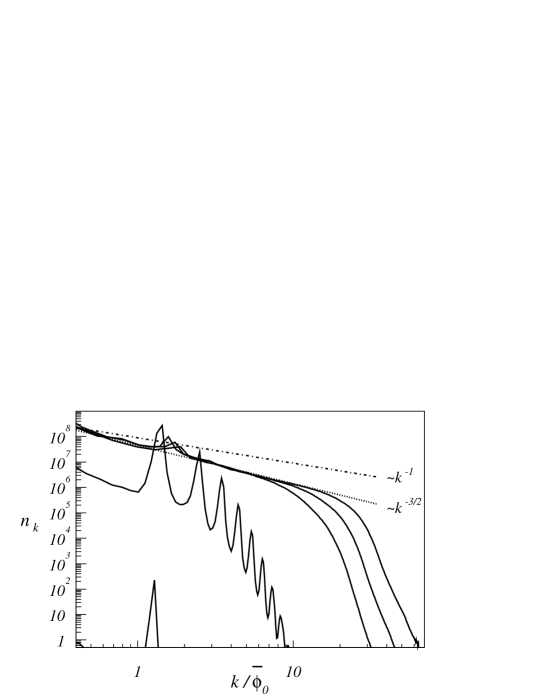
Figure 2: Occupation numbers as function of $k/\overline{\phi}_{0}$ at $\tau=100,400,2500,5000,10000$.

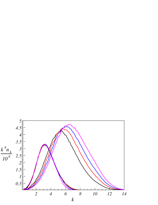
Figure 3: On the right hand side we plot the wave energy per decade found in lattice integration at $\tau=3600,5100,7000,10000$. On the left hand side are the same graphs transformed according to the relation inverse to Eq. (5).

3.3 Discussion

Let us see if these numerical results can be understood analytically. Features (1) and (2) facilitate the use of a simple kinetic approach, $\dot{n_{k}}=I_{k}$, where the collision integral for a $m$-particle interaction is given by[9]

$$I_{k}=\int d\Omega_{k}\,U_{k}\,F[n]\,.$$ (6)

In $d$ spatial dimensions the integration measure $d\Omega_{k}$ corresponds to $m-1$ integrations over $d$-dimensional Fourier space. Included in it is the energy-momentum conservation $\delta$-functions but not the relativistic $1/\omega(k_{i})$ “on-shell” factors, which instead appear in the “matrix element” of the corresponding process, $U_{k}$. This convention makes the discussion of relativistic and non-relativistic cases uniform. The function $F[n]$ is a sum of products of the type $n_{k_{j}}^{-1}\prod_{i=1}^{m}n_{k_{i}}$, where $j\in\{1,\dots,m\}$ with appropriate signs and permutations of indices for incoming and outgoing particles. All dynamical aspects of turbulence follow from the scaling properties of the system[19, 20]. Let $\omega_{k},n_{k}$ and $U_{k}$ have defined weights under a $\xi$-rescaling of the Fourier space,

$$\omega(\xi k_{i}) = \xi^{\alpha}\omega(k_{i})\;,$$

$$U(\xi k_{1},\dots,\xi k_{m}) = \xi^{\beta}U(k_{1},\dots,k_{m})\;,$$

$$n(\xi k_{i}) = \xi^{\gamma}n(k_{i})\;.$$ (7)

The weight of the full collision integral under this reparametrization is

$$I_{\xi k}=\xi^{d(m-2)-\alpha+\beta+(m-1)\gamma}I_{k}\,.$$ (8)

Then stationary turbulence with constant energy flux over momentum space is characterised by a power-law distribution function, $n_{k}\sim k^{-s}$, where $s=d+\beta/({m-1})$. The scaling properties also give the exponents of the self-similar distribution, Eq. (5). A system with energy conservation in particles and $\xi=\tau^{-p}$ has $q=4p$ and $p=1/((m-1)\alpha-\beta)$, while for stationary turbulence exponent $p$ should be $(m-1)$ times larger.

For a massless $\lambda\phi^{4}$-theory in three spatial dimensions and four-particle interaction we have $m=4$, $\beta=-4\alpha$ and $\alpha=1$. In this case $s=5/3$ and $p=1/7$ [9]. Obtained value for p is somewhat smaller then observed numerically, $p=1/5$. For three-particle interaction (the fourth particle belongs to the condensate in this case and the matrix element contains an additional factor $\overline{\phi}_{0}^{2}$) the stationary turbulence is characterized by $s=3/2$ and $p$ has even smaller value compared to 4-particle interaction. Numerical results[9] do not allow to distinguish between $5/3$ and $3/2$, $s$ rather fluctuates between these two numbers, while $1/7$ for $p$ gives a fit to the data not as good as displayed in Fig. 3. However, taking into account the non-stanionarity of the source (influx of energy from the zero-mode is still non-negligible) we obtain $q\approx 3.5p$ and $p\approx 1/6$ [9]. This should be considered as satisfactory agreement between numerical experiment and a theory, given the simplifications which were made.

3.4 Equilibration time and temperature

At late times, with decreased influence of the zero-mode, our simple analytical description should become more precise. On the other hand we can expect that the self-similarity persists. In this case solution Eq. (5) with $p=1/7$, which determines the transport of energy to higher momenta, should be valid. In classical frameworks it will be valid at all later times. Therefore, the time needed to reach equilibrium can be defined as the time when classical approximation breaks down. In other words, equilibrium will be reached after occupation numbers in the region of the peak, see Fig. 3, will become of order one. Using Eq. 5 we find[9] for the equilibration time $\tau\sim\lambda^{-7/4}\sim 10^{23}$, where in the second equality the normalization to the inflationary model is assumed. Rotating back from the conformal reference frame, we obtain for the reheating temperature $T_{R}\sim k_{max}/a(\tau)\sim\lambda^{2}\varphi_{0}(t_{0})\sim 10^{-26}M_{\rm Pl}\sim 100$ eV [9]. This result coinsides with what could have been obtained in “naive” perturbation theory. Namely, equating the rate of scattering in thermal equilibrium to the Hubble expansion rate we get in this model $T\sim\lambda^{2}M_{\rm Pl}$.

4 Conclusions

Reheating after preheating appears to be a rather slow process. Although the “effective temperature” measured at low momentum modes during preheating may be high, in the model we have considered the resulting true temperature is parametrically the same as what could have been obtained in “naive” perturbation theory. We anticipate this result should be applicable to more realistic models of inflation. Note that realistic models involve many fields and interactions and the largest coupling constants will determine the true temperature.

References

- [1] A.D. Linde, Particle Physics and Inflationary Cosmology, (Harwood Academic, New York, 1990); E. W. Kolb and M. S. Turner, The Early Universe, (Addison-Wesley, Reading, Ma., 1990); A.R. Liddle, D.H. Lyth, Cosmological Inflation and Large-Scale Structure, (Cambridge University Press, Cambridge, 2000 ); D. H. Lyth and A. Riotto, Phys. Rept. 314, 1 (1999).
- [2] E. W. Kolb, A. D. Linde and A. Riotto, Phys. Rev. Lett. 77, 4290 (1996); E. W. Kolb, A. Riotto and I. I. Tkachev, Phys. Lett. B 423, 348 (1998); J. Garcia-Bellido et al, Phys. Rev. D 60, 123504 (1999); J. Garcia-Bellido and E. Ruiz Morales, Phys. Lett. B 536, 193 (2002).
- [3] I. Affleck and M. Dine, Nucl. Phys. B 249, 361 (1985).
- [4] J. R. Ellis, A. D. Linde and D. V. Nanopoulos, Phys. Lett. B 118, 59 (1982); J. R. Ellis, D. V. Nanopoulos and S. Sarkar, Nucl. Phys. B 259, 175 (1985).
- [5] D. J. Chung, E. W. Kolb and A. Riotto, Phys. Rev. D 59, 023501 (1999); V. Kuzmin and I. Tkachev, JETP Lett. 68, 271 (1998) and Phys. Rev. D 59, 123006 (1999).
- [6] D. T. Son, Phys. Rev. D 54, 3745 (1996); D. V. Semikoz, Helv. Phys. Acta 69, 207 (1996); G. Aarts, G. F. Bonini and C. Wetterich, Nucl. Phys. B 587, 403 (2000); S. Davidson and S. Sarkar, JHEP 0011, 012 (2000); M. Salle, J. Smit and J. C. Vink, Phys. Rev. D 64, 025016 (2001); E. Calzetta and M. Thibeault, Phys. Rev. D 63, 103507 (2001); M. Grana and E. Calzetta, Phys. Rev. D 65, 063522 (2002); G. Aarts et al, Phys. Rev. D 66, 045008 (2002); J. Berges and J. Serreau, hep-ph/0208070.
- [7] S. Y. Khlebnikov and I. I. Tkachev, Phys. Rev. Lett. 77, 219 (1996); ibid 79, 1607 (1997); Phys. Lett. B 390, 80 (1997).
- [8] G. N. Felder and L. Kofman, Phys. Rev. D 63, 103503 (2001).
- [9] R. Micha and I. I. Tkachev, arXiv:hep-ph/0210202.
- [10] L. Kofman, A. D. Linde and A. A. Starobinsky, Phys. Rev. Lett. 73, 3195 (1994); Y. Shtanov, J. Traschen and R. H. Brandenberger, Phys. Rev. D 51, 5438 (1995).
- [11] L. Kofman, A. D. Linde and A. A. Starobinsky, Phys. Rev. D 56, 3258 (1997); P. B. Greene at al, Phys. Rev. D 56, 6175 (1997).
- [12] T. Prokopec and T. G. Roos, Phys. Rev. D 55, 3768 (1997).
- [13] J. Garcia-Bellido and A. D. Linde, Phys. Rev. D 57, 6075 (1998); R. Micha and M. G. Schmidt, Eur. Phys. J. C 14, 547 (2000); G. N. Felder et al, Phys. Rev. Lett. 87, 011601 (2001).
- [14] J. Baacke, K. Heitmann and C. Patzold, Phys. Rev. D 58, 125013 (1998); P. B. Greene and L. Kofman, Phys. Lett. B 448, 6 (1999).
- [15] G. F. Giudice et al, JHEP 9908, 014 (1999).
- [16] L. Kofman, A. D. Linde and A. A. Starobinsky, Phys. Rev. Lett. 76, 1011 (1996); I. I. Tkachev, Phys. Lett. B 376, 35 (1996); S. Khlebnikov et al, Phys. Rev. Lett. 81, 2012 (1998).
- [17] S. Y. Khlebnikov and I. I. Tkachev, Phys. Rev. D 56, 653 (1997).
- [18] G. N. Felder and I. Tkachev, LATTICEEASY code, arXiv:hep-ph/0011159.
- [19] A. K. Kolmogorov, Dokl. Akad. Nauk. SSSR 30, 9 (1941); A. V. Kats, Zh. Eksp. Teor. Fiz. 71, 2104-2112 (1976); V. E. Zakharov, S. L. Musher, A. M. Rubenchik, Phys. Rep. 129, 285 (1985); G. E. Falkovich and A. V. Shafarenko, J. Nonlinear Sci. 1, 457 (1991); V. Zakharov, V. L’vov, G. Falkovich, Kolmogorov Spectra of Turbulence, Wave turbulence. Springer-Verlag 1992.
- [20] D. V. Semikoz and I. I. Tkachev, Phys. Rev. Lett. 74, 3093 (1995) D. V. Semikoz and I. I. Tkachev, Phys. Rev. D 55, 489 (1997)