Popping out the Higgs boson off vacuum at Tevatron and LHC

Abstract

In the prospect of diffractive Higgs production at the LHC collider, we give an extensive study of Higgs boson, dijet, diphoton and dilepton production at hadronic colliders via diffraction at both hadron vertices. Our model, based on non factorizable Pomeron exchange, describes well the observed dijet rate observed at Tevatron Run I. Taking the absolute normalization from data, our predictions are given for diffractive processes at Tevatron and LHC. Stringent tests of our model and of its parameters using data being taken now at Tevatron Run II are suggested. These measurements will also allow to discriminate between various models and finally to give precise predictions on diffractive Higgs boson production cross-section at the LHC.

1 Double Diffractive Hard Production through non-factorizable Vacuum Exchange

The discovery of the Higgs boson is one of the main goals of searches at the present and next hadronic colliders, the Tevatron and the LHC. The standard, non-diffractive production mechanisms are being studied extensively. The main decay modes of a low-mass Higgs boson are $b$-quark pairs and $\tau$-leptons, which are difficult to extract from the standard model background processes. A promising channel is the $\gamma\gamma$ decay mode; however, due to the small branching fraction (about 10^-3), a luminosity of the order of 50 fb^-1 is needed to establish the existence of the Higgs boson in the mass range below 135 GeV. It is thus important to investigate other, complementary ways to produce and detect the Higgs boson in this mass range.

One promising production mode, the exclusive double diffractive production, was proposed some time ago in Ref. [1, 2]. In this case, the Higgs boson is diffractively produced in the central region resulting in a final state composed of the two protons scattered at very small angles and detected in the roman pot detectors, the decay products of the Higgs boson in the main detector, and nothing else. It is thus a very clean signal. The kinematic constraints coming from the proton detection in the roman pot detectors allow a very precise determination of the Higgs boson mass [3], hence improving the signal to background ratio. Contrary to non-diffractive production, the main Higgs boson decay modes, like $b\bar{b}$ or $\tau\tau$ are thus promising channels. However, the exclusive cross-sections may be very low, and thus put strong limitations to the potentialities of double diffractive production.

Recently, we have studied the possibility of producing the Higgs boson together with other particles, i.e. inclusive diffractive production [4]. The expected cross-sections are increased compared to exclusive production, and the model can be “calibrated” using the diffractive dijet production measured by the CDF Collaboration at Tevatron run I [5]. The experimental result, and in particular the dijet mass fraction spectrum, shows that hadronic activity in the central region (coming from hard QCD radiation, and from soft Pomeron remnants) needs to be accounted for, in order to describe these data. We have proposed a model for double diffractive production of heavy “objects”, based on a non-factorizable Pomeron model and able to describe the observed features of dijet production data in a qualitative way. Normalizing our raw predictions to the CDF measurement allows to make quantitative predictions for the Tevatron and the LHC, given specific assumptions for the model parameters. We have also shown [6] that it is possible to reconstruct precisely the mass of the Higgs boson if both protons in the final state can be detected with roman pot detectors and if the Pomeron remnants can be measured in the forward region with sufficient resolution.

At the Tevatron collider, the Higgs boson production cross-section is severely limited by the small available phase space. At the LHC, since the beam energy is much higher, diffractive Higgs boson production has larger cross-section, and might thus be an interesting channel, as we shall discuss further on. On the other hand, even if double diffractive Higgs boson production at the Tevatron is probably too small by itself, it is however possible to verify and constrain models of double diffraction at the Tevatron Run II, through the study of difermion production.

In this paper, we wish to provide an extensive study of our model, including predictions for dijet, diphoton and dilepton production and their ratios for both the Tevatron run II and the LHC. We will discuss possible values of its characteristic parameters, and propose means to discriminate between the existing models at the Tevatron. In turn, this study will help to formulate more precise predictions for double diffractive Higgs boson production at the LHC in the near future.

The plan of our study is the following. In Section 2, we will recall and discuss the original exclusive model of Bialas and Landshoff [1], and our extension to inclusive production. In Section 3 predictions are given for dijet, diphoton, dilepton and Higgs boson cross-sections. Dijet results for the Tevatron run I, using a fast simulation of detector effects, are in good agreement with available data and are used to normalize our predictions. A discussion of Pomeron remnants and their possible detection is also given. In Section 4, ways to verify our model and determine its parameters using Tevatron data are proposed. The possibility of distinguishing our model from the existing models of double diffraction is discussed in Section 5. Section 6 summarizes the interest of diffractive Higgs boson production compared to standard production. Finally, Section 7 gives conclusions and an outlook on the promising future studies on hard diffraction production at the Tevatron and the LHC.

2 Inclusive vs. exclusive production

2.1 Exclusive production

Let us first introduce the original model of [1] describing exclusive Higgs boson and $q\bar{q}$ production in double diffractive production (noted DPE in the following). This process is depicted in Fig. 1, “Exclusive” case.

In [1], the diffractive mechanism is based on two-gluon exchange between the two incoming protons. The soft Pomeron is seen as a pair of gluons non-perturbatively coupled to the proton. One of the gluons is then coupled perturbatively to the hard process (either the Higgs boson, or the $q\bar{q}$ pair, see Fig. 1), while the other one plays the rôle of a soft screening of color, allowing for diffraction to occur. This soft character requires the phenomenological introduction of a distinctive non-perturbative gluon propagator [7] whose parameters are constrained by the description of total cross-sections using the same formalism.

The hard gluons, carrying all remaining momentum ($x_{1}^{g}=x_{2}^{g}=1$), fuse to produce the heavy object (Higgs boson and diquarks in the original model). The corresponding cross-sections for $q\bar{q}$ and Higgs boson production read:

$$d\sigma_{q\bar{q}}^{exc}(s) = C_{q\bar{q}}^{exc}\left(\frac{s}{M_{q\bar{q}}^{2}}\right)^{2\epsilon}\delta^{(2)}\left(\sum_{i=1,2}(v_{i}+k_{i})\right)\prod_{i=1,2}\left\{d^{2}v_{i}d^{2}k_{i}d\eta_{i}\ \xi_{i}^{2\alpha^{\prime}v_{i}^{2}}\!\exp(-2\lambda_{JJ}v_{i}^{2})\right\}{\sigma^{exc}_{q\bar{q}}};$$

$$d\sigma_{H}^{exc}(s) = C_{H}\left(\frac{s}{M_{H}^{2}}\right)^{2\epsilon}\delta\left(\xi_{1}\xi_{2}-\frac{M_{H}^{2}}{s}\right)\prod_{i=1,2}\left\{d^{2}v_{i}\frac{d\xi_{i}}{1-\xi_{i}}\ \xi_{i}^{2\alpha^{\prime}v_{i}^{2}}\exp(-2\lambda_{H}v_{i}^{2})\right\}\ .$$ (1)

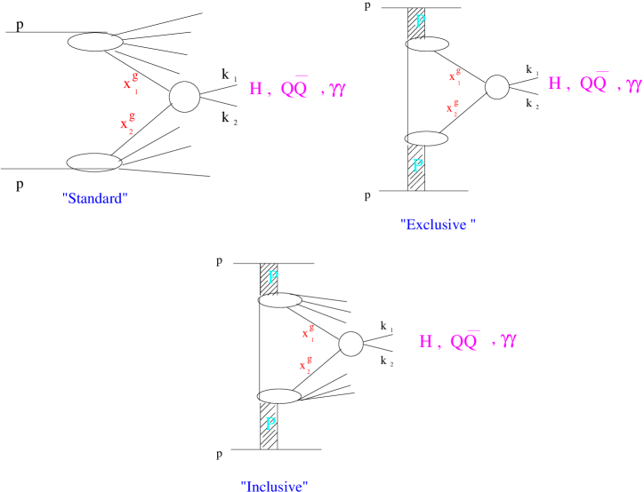
Figure 1: Double diffractive vs. standard gluon fusion production schemes. $x_{i}^{g}$ are the momentum fractions of the fusing gluons, $k_{i}$ are the transverse 2-momenta of the outgoing difermion in the central rapidity region. The “Standard” Higgs boson production is displayed for reference. “Exclusive” and “inclusive” double diffraction are represented in the framework of the non factorizable Pomeron model (see formulae (1,4-7) and text for the complete kinematical notations). The hatched region represents the diffractive interactions at both (anti)proton vertices, while the vertical thin line is for the soft gluon exchange in the model. Note that $x_{i}^{g}\equiv 1$ in the “exclusive” case.

The variables $v_{i}$ and $k_{i}$ respectively denote the transverse momenta of the outgoing protons and quarks, $\xi_{i}$ are the proton fractional momentum losses, and $\eta_{i}$ are the quark rapidities. $\sigma_{H}$ is the gluon-initiated Higgs boson production cross-section while ${\bar{\sigma}_{q\bar{q}}}^{exc}$ is the hard $q\bar{q}$ production cross-section in the exclusive case. Indeed, in this exclusive process submitted to the $J_{Z}=0$ constraint [8] (a helicity selection rule for the production of a scalar system from the vacuum channel), the $q\bar{q}$ differential cross-section writes, apart from normalizations included in $C_{q\bar{q}}$:

$${\sigma}_{q\bar{q}}^{exc}\equiv\frac{\pi}{24}\frac{d\sigma}{dt}=\frac{\rho(1-\rho)}{m_{T1}^{2}m_{T2}^{2}}\,\,,\,\,\rho=\frac{4m_{Q}^{2}}{M_{q\bar{q}}^{2}}\ .$$ (2)

In the model, the non-perturbative input is naturally related to the soft Pomeron trajectory taken from the standard Donnachie-Landshoff parametrization [10], namely $\alpha(t)=1+\epsilon+\alpha^{\prime}t$, with $\epsilon\approx 0.08$ and $\alpha^{\prime}\approx 0.25\mathrm{GeV^{-2}}$.

There are other parameters to be fixed, coming from the non-perturbative gluon propagators. Phenomenological contraints are obtained from the physical values of the total cross-sections, leading to four unknown parameters in formula (1), namely the normalizations $C_{q\bar{q}},\ C_{H}$ and the slopes in momentum transfer $\lambda_{q\bar{q}},\lambda_{H}.$ At this point of our study, the slopes $\lambda_{q\bar{q}},\lambda_{H}$ are kept as in the original papers [1] .

The problem of the normalization constants $C_{q\bar{q}},\ C_{H}$ requires more care, since the evaluation of cross-sections is the main subject of the paper. All constants of the problem (non-perturbative proton-gluon coupling, normalization of the non-perturbative gluon propagators, color factors, perturbative Higgs boson and $q\bar{q}$ production vertices) are contained in the normalizations $C_{q\bar{q}}$ and $C_{H}$. The non-perturbative factors are poorly determined by the current data, implying large uncertainties on production cross-section predictions. In particular, even if every other parameter is fixed, the non-perturbative proton-gluon coupling $G$ remains undetermined and is arbitrarily fixed to $G^{2}/4\pi=1$ in the original publications [1]. However, and it is an important aspect of our model studies, the ratio $C_{H}/C_{q\bar{q}}$ is well defined, and independent of everything else than the color structure of the process. This means that the ratio of Higgs boson to diquark production is fixed by this factor. Given the expressions of $C_{H}$ and $C_{q\bar{q}}$ [1], one finds :

$$\left(\frac{C_{H}}{C_{q\bar{q}}}\right)=\frac{\sqrt{2}{\cal G}_{F}}{3\pi}\ ,$$ (3)

where enter only in (3) the Fermi constant ${\cal G}_{F}$, and the ratio of color factors to produce either a color singlet $q\bar{q}$ or the scalar Higgs boson in the non-factorizable Pomeron model (see for details, the second reference of [1]). This feature will remain valid in our model of inclusive production, suggesting that the known, large cross-section dijet production process can be used to calibrate Higgs boson production.

Also note that, as can be seen in (2), the exclusive production rate for a given quark flavour is proportional to its mass squared, so that light quark production is expected to be negligible, reflecting in another way the $J_{Z}=0$ constraint [8].

2.2 Inclusive production

The inclusive mechanism is described in the third graph of Fig. 1. The idea is to take into account that a Pomeron is a composite system, made itself from quarks and gluons. In our model, we thus apply the concept of Pomeron structure functions to compute the inclusive diffractive Higgs boson cross-section. The H1 measurement of the diffractive structure function [11] and the corresponding quark and gluon densities are used for this purpose. This implies the existence of Pomeron remnants and QCD radiation, as is the case for the proton. This assumption comes from QCD factorisation of hard processes. However, and this is also an important issue, we do not assume Regge factorisation at the proton vertices, i.e. we do not use the H1 Pomeron flux factors in the proton or antiproton.

Regge factorisation is known to be violated between HERA and the Tevatron. Moreover, we want to use the same physical idea as in the exclusive model [1], namely that a non perturbative gluon exchange describes the soft interaction between the incident particles, as in Fig. 1. In practice, the Regge factorisation breaking appears in three ways in our model:

i) We keep as in the original model of Ref [1] the soft Pomeron trajectory with an intercept value of 1.08.

ii) We normalize our predictions to the CDF Run I measurements, allowing for factorisation breaking of the Pomeron flux factors in the normalisation between the HERA and hadron colliders .

iii) The color factor (3) derives from the non-factorizable character of the model, since it stems from the gluon exchange between the incident hadrons. We will see later the difference between this and the factorizable case.

The formulae for the inclusive production processes considered here follow. We have, for dijet production, considering only the dominant gluon-initiated hard processes:

$$d\sigma_{JJ}^{incl}=C_{JJ}\left(\frac{x^{g}_{1}x^{g}_{2}s}{M_{JJ}^{2}}\right)^{2\epsilon}\!\!\!\!\delta^{(2)}\!\left(\sum_{i=1,2}v_{i}\!+\!k_{i}\right)\prod_{i=1,2}\!\!\left\{{d\xi_{i}}{dx_{i}^{g}}d^{2}v_{i}d^{2}k_{i}{\xi_{i}}^{2\alpha^{\prime}v_{i}^{2}}\!\exp\left(-2v_{i}^{2}\lambda_{JJ}\right)\right\}\times$$

$$\times\left\{{\sigma_{JJ}}G_{P}(x^{g}_{1},\mu)G_{P}(x^{g}_{2},\mu)\right\};$$ (4)

and for Higgs boson production:

$$d\sigma_{H}^{incl}=C_{H}\left(\frac{x^{g}_{1}x^{g}_{2}s}{M_{H}^{2}}\right)^{2\epsilon}\!\!\delta\left(\xi_{1}\xi_{2}\!-\!\frac{M_{H}^{2}}{x^{g}_{1}x^{g}_{2}s}\right)\!\!\prod_{i=1,2}\left\{G_{P}(x^{g}_{i},\mu)\ dx^{g}_{i}d^{2}v_{i}\ \frac{d\xi_{i}}{1\!-\!\xi_{i}}\ {\xi_{i}}^{2\alpha^{\prime}v_{i}^{2}}\ \exp\left(-2v_{i}^{2}\lambda_{H}\right)\right\};$$ (5)

For the two following processes, the quark-initiated contribution can not be ignored. We have, for dilepton production:

$$d\sigma_{ll}^{incl}=C_{ll}\left(\frac{x^{q}_{1}x^{q}_{2}s}{M_{ll}^{2}}\right)^{2\epsilon}\!\!\!\!{\sigma_{q\bar{q}\rightarrow ll}}\delta^{(2)}\!\left(\sum_{i=1,2}v_{i}\!+\!k_{i}\right)\!\!\prod_{i=1,2}\!\!\left\{Q_{P}(x^{g}_{i},\mu){d\xi_{i}}{dx_{i}^{g}}d^{2}v_{i}d^{2}k_{i}{\xi_{i}}^{2\alpha^{\prime}v_{i}^{2}}\!\exp\left(-2v_{i}^{2}\lambda_{ll}\right)\right\};$$ (6)

and for diphoton production:

$$d\sigma_{\gamma\gamma}^{incl}=C_{ll}\left(\frac{x^{g}_{1}x^{g}_{2}s}{M_{\gamma\gamma}^{2}}\right)^{2\epsilon}\!\!\!\!\delta^{(2)}\!\left(\sum_{i=1,2}v_{i}\!+\!k_{i}\right)\prod_{i=1,2}\!\!\left\{{d\xi_{i}}{dx_{i}^{g}}d^{2}v_{i}d^{2}k_{i}{\xi_{i}}^{2\alpha^{\prime}v_{i}^{2}}\!\exp\left(-2v_{i}^{2}\lambda_{\gamma\gamma}\right)\right\}\times$$

$$\times\left\{{\sigma_{gg\rightarrow\gamma\gamma}}G_{P}(x^{g}_{1},\mu)G_{P}(x^{g}_{2},\mu)+\sigma_{q\bar{q}\rightarrow\gamma\gamma}Q_{P}(x^{g}_{1},\mu)Q_{P}(x^{g}_{2},\mu)\right\}.$$ (7)

In the above, $x_{i}^{g}$ are the Pomeron’s momentum fractions carried by the gluons or quarks involved in the hard process, and the $G_{P}$ (resp. $Q_{P}$) are the Pomeron gluon (resp. quark) energy densities, $i.e.$ the parton density multiplied by $x_{i}^{g}$. We use as parametrizations of the Pomeron structure functions the fits to the diffractive HERA data performed in [14]. The dijet cross-section is now (summing over quark flavours $f$, and now including the contribution from gluon jets):

$${\sigma}_{JJ}=\sum_{f}{\sigma}_{gg\rightarrow q\bar{q}}(\rho^{f})+108\ {\sigma}_{gg\rightarrow gg}(\rho^{g})\,\,;\,\,\rho^{f}=\frac{4m^{f}_{T1}m^{f}_{T2}}{M_{JJ}^{2}}\,\,\ ;\,\,\rho^{g}=\frac{4p_{T1}p_{T2}}{M_{JJ}^{2}};$$

$${\sigma}_{gg\rightarrow q\bar{q}}=\frac{\rho^{f}}{{m^{f}_{T1}}^{2}{m^{f}_{T2}}^{2}}\left(1-\frac{\rho^{f}}{2}\right)\left(1-\frac{9\rho^{f}}{16}\right)\,\,;\,\,{\sigma}_{gg\rightarrow gg}=\frac{1}{p_{T1}^{2}p_{T2}^{2}}\left(1-\frac{\rho^{g}}{4}\right)^{3};$$ (8)

to be compared with (2). The above formulae are derived using [16], and the dilepton and diphoton cross-sections are taken from [17, 18]. The expressions for $\sigma_{gg\rightarrow q\bar{q}},\sigma_{gg\rightarrow gg},\sigma_{q\bar{q}\rightarrow ll},$ and $\sigma_{gg\rightarrow\gamma\gamma},\sigma_{q\bar{q}\rightarrow\gamma\gamma}$ in terms of the Mandelstam variables are recalled in the Appendix.

In the inclusive case, contrary to the exclusive case, dijet production is flavour democratic and thus the $\sum_{f}$ in (8) extends over all flavors except for the too massive top quark, due to kinematics. Note that the non perturbative parameters are kept the same as in the exclusive case. Indeed, the expressions (1) can be recovered in the limit $G_{P}\rightarrow\delta(x-1)$, and substituting back equation (2) instead of (8) for the hard cross-section, which restricts to the $J_{Z}=0$ component of the $q\bar{q}$ cross-section and reintroduces the flavor mass hierarchy. The normalization of $G_{P}$ is not determined by the HERA data (since it is mixed with the flux factors) but is fixed in the model in order to lead to the same result for the energy-momentum sum rule as for the exclusive case. It is interesting to note that the comparison with the observed dijet production rates will give the correct order of magnitude for the inclusive model, while the exclusive one leads to too important rates, as discussed in the next section. Note that the normalization cancels in the ratio $\left(\frac{C_{H}}{C_{JJ}}\right)$, with the same value as in the exclusive case, see 3.

3 Model predictions for DPE

3.1 DPE Dijets at the Tevatron Run I

The CDF measurement of double diffractive dijet production [5] is used as a verification of the validity of our approach (namely concerning the inclusive picture we consider, and the application of structure functions measured in electron-proton collisions in our context). Once the model validity tested, the measured cross-section will allow us to fix (within experimental errors) the absolute normalization of the cross-sections.

In the CDF measurement, an outgoing antiproton is measured on one side of the detector, and the DPE nature of the events is ensured by requiring a rapidity gap on the opposite side. The selection then requires at least two jets satisfying a transverse energy criterion. The details of the selections can be found in [5]. The measured cross-section is $43.6\pm 4.4\mathrm{(stat)}\pm 21.6\mathrm{(syst)}$ nb, with large error bars.

Reproducing the experimental selections on the cross-section estimates, and keeping fixed all parameters as in the exclusive case we obtain a raw prediction of 11.4 nb, i.e. a factor 3.8 smaller than the measured mean value . This prediction includes a fast simulation of detector resolution effects, using SHW [19]. Considering the large uncertainties, this result is quite encouraging. Indeed, as mentioned above, the experimental errors are yet quite large.

In order to verify the dynamics of the model, it is interesting to consider the dijet mass fraction, defined as the ratio of the mass measured in the central detector to the missing mass to the outgoing proton and antiproton. For exclusive events, this ratio is expected to be about 0.8 [5] given detector inefficiencies; if inclusive events dominate, and the model is correct, one should observe a broad distribution below one, essentially given by the product of the Pomeron structure functions. Fig. 3 displays the mass fraction as measured by CDF, and the prediction of the present model .

Reasonable agreement is observed, suggesting that the HERA Pomeron structure functions allow for a correct description of inclusive DPE events. It is worthwhile to emphasize the strong influence of the behaviour of the (hard) gluon distribution of the Pomeron on the predicted mass fraction. In Fig. 3, we consider a “proton-like” ($i.e$, soft) gluon distribution in the Pomeron, leading to unsatisfactory results.

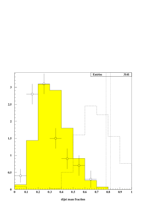
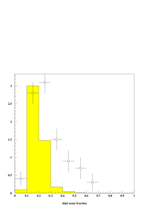
Figure 2: Observed dijet mass fraction (CDF Run I), compared to our model prediction, using the Pomeron structure functions. The dashed histograms are for exclusive production with and without ($cf.$ the peak at 0.8) detector simulation.

Figure 3: Dijet mass fraction obtained using the gluon structure function from the proton.

3.2 Model predictions for Tevatron and LHC: dijets, diphotons and dileptons

Assuming a global normalization as determined here and all other model parameters as given above, one is now in situation to give predictions for Higgs boson production at the Tevatron and the LHC. In a first stage, we assume no evolution of this normalization with energy. We will discuss later on the influence of the various parameters on the predictions, analyze the (large) uncertainties which still affect the results and, above all, what can be done in the future to handle them, both on experimental and theoretical grounds. For this sake, after scaling our model to the CDF Tevatron run I predictions, we give predictions for various DPE processes which are relevant for Tevatron Run II and LHC measurements.

In Figs. 4 and 5, we give the integrated cross sections for dijets, quarks, $b\bar{b}$, dileptons and diphotons at generator level for a mass higher than the mass $m$ given on the abscissa for the Tevatron and the LHC. Each figure is displayed for two different mass ranges, namely between 10 and 100 GeV, and 100 and 160 GeV.

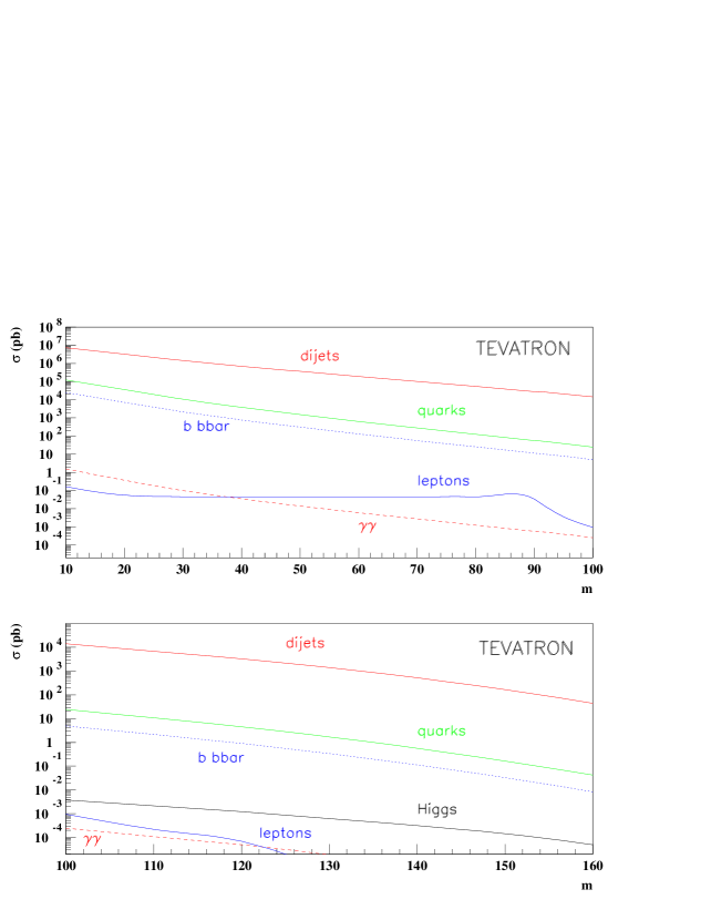
Figure 4: Dijet, diquark, $b\bar{b}$, dilepton, and diphoton cross-sections (pb) at the Tevatron. The cross-sections are given for a mass $m$ above the value on the abscissa, for two different mass ranges. For comparison, we also display the Higgs boson cross-section for $M_{Higgs}=m$.

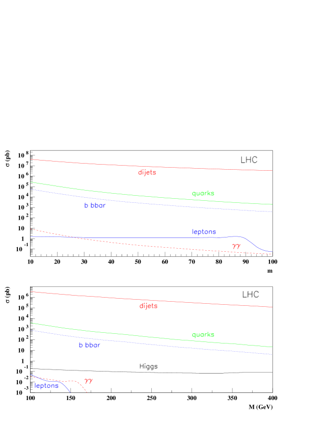
Figure 5: Dijet, diquark, $b\bar{b}$, dilepton, and diphoton cross-sections (pb) at the LHC. The cross-sections are given for a mass $m$ above the value on the abscissa, for two different mass ranges. For comparison, we also display the Higgs boson cross-section for $M_{Higgs}=m$.

The differential cross-sections for dijet, dilepton and diphoton production are also given in Fig. 7 and 7. The dijet cross-section is dominated by the gluon contribution. The quark jet contribution amounts 1% at small masses, and goes down to 0.1% at higher masses, both at the Tevatron and the LHC. The $b\bar{b}$ contribution, which is about 20% of the total quark contribution, represents only about 0.02% of the dijet yield. The diphoton cross-section is small (4 orders of magnitude below the $b\bar{b}$ cross-section both at Tevatron and LHC) but still measurable at Tevatron at low masses to test the model. These processes are much smaller than dijet production (due to the weak QED coupling constant, and to the small quark component of the Pomeron which initiates these processes), but they do have appreciable advantages which will appear in the following discussion. The dilepton cross-section is small (same order of magnitude as the diphoton) but enhanced by the presence of the $Z$ pole (see Fig. 7). Numerical values for the cross-sections are also given in Table 1.

Process	(1)	(2)	(3)	(4)
Dijets	$7.010^{5}$	$3.210^{3}$	$1.210^{7}$	$2.510^{6}$
Diquarks	$3.810^{3}$	$4.4$	$3.610^{4}$	$1.710^{3}$
$b\bar{b}$	$7.610^{2}$	$8.710^{-1}$	$9.410^{3}$	$4.510^{2}$
$\gamma\gamma$	$3.510^{-2}$	$4.910^{-5}$	$4.410^{-1}$	$1.910^{-2}$
$l^{+}l^{-}$	$4.610^{-2}$	$6.810^{-5}$	$1.1$	$1.310^{-2}$

Table 1: DPE cross-section (pb) for dijets, diquarks, $b\bar{b}$, diphotons and dileptons (fb). (1): at the Tevatron, $|y|<5$, $m>40$ GeV; (2): at the Tevatron, $|y|<5$, $m>120$ GeV; (3): at the LHC, $|y|<5$, $m>40$ GeV; (4): at the LHC, $|y|<5$, $m>120$ GeV.

Figure 6: Differential dijet production cross-section (pb) at the Tevatron and the LHC. The transverse energy of the central jets satisfies $E_{T}>10$ GeV, and their rapidity is limited to $|y|<4$.

Figure 7: Differential diphoton and dilepton production cross-sections (fb) at the Tevatron and the LHC. The dilepton cross-section corresponds to a single lepton flavour. The transverse energy of the central particles satisfies $E_{T}>10$ GeV, and their rapidity is limited to $|y|<4$.

3.3 Model predictions for the Tevatron and the LHC: Higgs boson production

Our results for Higgs boson production at the Tevatron and the LHC are displayed in Figs. 8, 10 and 10, and in Tables 2 and 3. In Fig. 8, we see that the Higgs production cross-section at the LHC is higher by more than two orders of magnitude than at the Tevatron. In the same figure is also displayed for comparison the cross-section for standard Higgs production, which is more than two orders of magnitude larger. In Figs. 10 and 10, we give the Higgs boson production cross section at the Tevatron and the LHC for the different decay modes of the Higgs boson.

$M_{H}$	(1)	(2)	(3)	(4)
100	3.8	3.2	0.3	0.0
110	2.3	1.8	0.2	0.0
120	1.3	0.9	0.1	0.1
130	0.7	0.4	0.0	0.2
140	0.3	0.1	0.0	0.2

Table 2: DPE Higgs production cross-section at the Tevatron (fb). (1): total cross-section, (2): $b\bar{b}$ channel, (3): $\tau\tau$ channel, (4): $W^{+}W^{-}$ channel.

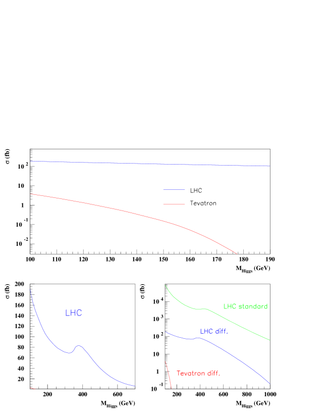
Figure 8: Higgs boson production cross-section at the LHC and the Tevatron. The upper plot gives the cross-sections at the Tevatron and the LHC for low Higgs mass to show the difference between both accelerators. The bottom plots show the same distribution at higher Higgs masses (the standard Higgs production cross-section is shown for comparison).

Figure 9: Higgs boson production cross-section at the Tevatron. Various decay channels are plotted as a function of the Higgs boson mass.

Figure 10: Higgs boson production cross-section at the LHC. Various decay channels are plotted as a function of the Higgs boson mass.

The diffractive Higgs production at the LHC is mainly interesting for the lower Higgs boson masses. When the Higgs boson mass is heavy enough, the $WW$ and $ZZ^{(*)}$ decay modes become dominant and the visibility of the corresponding channels are already very good in standard non-diffractive events ; hence we do not expect the contribution from diffractive channels to be as important there.

At lower Higgs masses, the standard non-diffractive searches are done using the $\gamma\gamma$ decay mode, which is loop-mediated and has very small branching fraction. In the present case, the good mass resolution obtained using roman pots or microstation detectors [21] allows to use the Higgs boson decays into b-quarks and into $\tau$-leptons, which are the two main decay modes when the Higgs boson is lighter than $\sim 140{\mathrm{G}eV/c^{2}}$. We will discuss this point in more detail later in this paper.

$M_{H}$	(1)	(2)	(3)	(4)
100	182.3	152.1	12.4	1.5
110	172.6	138.2	11.4	6.4
120	158.5	114.3	9.6	18.1
130	147.0	85.2	7.2	37.6
140	137.7	54.3	4.6	61.6
150	127.5	26.8	2.3	83.4
160	122.5	6.2	0.5	109.0
170	115.3	1.3	0.1	110.8
180	108.9	0.8	0.1	101.4
190	103.8	0.5	0.0	81.3
200	98.1	0.3	0.0	72.5

Table 3: DPE Higgs production cross-section at the LHC (fb). (1): total cross-section, (2): $b\bar{b}$ channel, (3): $\tau\tau$ channel, (4): $W^{+}W^{-}$ channel.

4 Parameter dependence of DPE cross-sections

In this section, we study the dependence of our predictions for dijet, diphoton, dilepton and Higgs boson cross-sections on the different parameters of the model. If we refer to the formulae given in the first section, the relevant parameters of our models are the momentum transfer slopes $\lambda_{i}$ (where $i$ stands for H, JJ, ll, qq, $\gamma\gamma$), and $\epsilon$ and $\alpha^{\prime}$ respectively the intercept and slope of the Pomeron Regge trajectory. We will discuss the dependence on $\epsilon$ in the next section (note that this value is however imposed in our model, but changes in other Pomeron models, as discussed later on).

The dependence on $\lambda_{H}$, $\lambda_{i}$ (where $i$ stands for $ll$, $JJ$, $b\bar{b}$, $qq$, and $\gamma\gamma$) is displayed in Tables 4 (for Tevatron) and 5 (for LHC). In our model, we assumed $\lambda_{H}=2$ and $\lambda_{i}=3$ (as in the original exclusive model [1]). We now vary these values by one unity, keeping values (assuming or not the equality of the $\lambda$’s) around those physically connected to the nucleon form factors. We also give numbers with the pomeron slope $\alpha^{\prime}$ taken to be 0.1. We note as expected that the cross-sections for dilepton, diphoton, dijet and $b\bar{b}$ production vary by the same factor when we vary the parameters.

The results of Tables 4 and 5 are shown for each value of the $\lambda$’s (except the reference one on the first row) on two lines: on the first line, we give the cross-section values as they come directly from the generator simulation, and on the second lines we rescale the values to the reference dijet cross-section. This method allows us to determine the error on the Higgs production cross-section due to the assumptions made on the respective values of $\lambda_{H}$ and $\lambda_{i}$. For the Tevatron, the cross-section we obtain for a Higgs boson mass of 120 GeV is 1.2 fb, and varies between 0.6 and 1.9, which gives an incertitude of about 50% on the Higgs boson cross-section prediction. For the LHC, the default value is 160 fb and varies between 89 and 220, which gives also an error of about 50%.

The other assumption in our study is to take the gluon density in the pomeron at $Q^{2}=75$ GeV², since this is the upper value of $Q^{2}$ for the QCD fit. If we take a value at a higher $Q^{2}$ by using a DGLAP evolution we obtain that the gluon density can vary by a factor 2 at $Q^{2}=4000$ GeV². This has a clear effect on our predictions which can thus vary by a factor 2.

Another assumption of our model which needs to be tested against data is that the fraction of events with tagged protons is the same at the LHC and the Tevatron, which in other words means that the gap survival probability does not depend much on the center of mass energy. To verify this point will be possible only when the LHC energy range will be available to experimentation.

To summarize, we estimate that, on the basis of our model calculations, the errors due to the parameter dependence on our predictions for Higgs cross section (once normalized to dijets) are of the order of a factor 4.

Param.	$\sigma_{dijets}$	$\sigma_{b\bar{b}}$	$\sigma_{\gamma\gamma}$	$\sigma_{ll}$	$\sigma_{Higgs}$
$\lambda_{H}=2$, $\lambda_{i}=3$	7.2 106	2.5 104	1.6	1.6 102	1.2
$\lambda_{H}=3$, $\lambda_{i}=4$	4.7 106	1.6 104	1.0	1.2 102	0.7
	7.2 106	2.4 104	1.5	1.8 102	1.1
$\lambda_{H}=2$, $\lambda_{i}=2$	1.3 107	4.5 104	2.8	3.3 102	1.2
	7.2 106	2.5 104	1.5	1.8 102	0.7
$\lambda_{H}=4$, $\lambda_{i}=4$	4.7 106	1.6 104	1.0	1.2 102	0.42
	7.2 106	2.4 104	1.5	1.8 102	0.64
$\lambda_{H}=1$, $\lambda_{i}=2$	1.3 107	4.5 104	2.8	3.3 102	3.5
	7.2 106	2.5 104	1.5	1.8 102	1.9
$\alpha^{\prime}=0.1$	9.8 106	3.4 104	2.2	2.5 102	1.8
	7.2 106	2.5 104	1.6	1.8 102	1.3

Table 4: Numerical values of the cross-sections (fb) for different values of the parameters, at the Tevatron
(the subscript $i$ stands for $ll$, $b\bar{b}$, $JJ$, $\gamma\gamma$). The Higgs cross-section is for a Higgs mass of 120 GeV. All other cross-sections are given for a dijet, dilepton, or diphoton mass greater than 10 GeV. The first lines read the direct output of the program, whereas the second lines are rescaled to the same value of the dijet cross-section, namely the CDF measurement.

Param.	$\sigma_{dijets}$	$\sigma_{b\bar{b}}$	$\sigma_{\gamma\gamma}$	$\sigma_{ll}$	$\sigma_{Higgs}$
$\lambda_{H}=2$, $\lambda_{i}=3$	4.2 107	1.1 105	8.8 103	1.6 103	1.6 102
$\lambda_{H}=3$, $\lambda_{i}=4$	2.7 107	7.5 104	5.5 103	1.0 103	9.0 101
	4.2 107	1.2 105	8.6 103	1.6 103	1.4 102
$\lambda_{H}=2$, $\lambda_{i}=2$	7.1 107	1.9 105	1.6 104	2.8 103	1.6 102
	4.2 107	1.1 105	9.5 103	1.7 103	9.5 101
$\lambda_{H}=4$, $\lambda_{i}=4$	2.7 107	7.5 104	5.5 103	1.0 103	5.7 101
	4.2 107	1.2 105	8.6 103	1.6 103	8.9 101
$\lambda_{H}=1$, $\lambda_{i}=2$	7.1 107	1.9 105	1.6 104	2.8 103	3.8 102
	4.2 107	1.1 105	9.5 103	1.7 103	2.2 102
$\alpha^{\prime}=0.1$	6.1 107	1.7 105	1.5 104	2.3 103	2.5 102
	4.2 107	1.2 105	1.0 104	1.6 103	1.7 102

Table 5: Numerical values of the cross-sections (fb) for different values of the parameters at the LHC ($i$ means $ll$, $b\bar{b}$, $JJ$, $\gamma\gamma$). The Higgs cross-section is for a Higgs mass of 120 GeV. All other cross-sections are given for a dijet, dilepton, or diphoton mass greater than 10 GeV. The first lines read the direct output of the program, whereas the second lines are rescaled to the same value of the dijet cross-section, namely the CDF measurement.

5 Testing and comparing models at the Tevatron Run II

Let us discuss and propose ways to verify our model and determine its parameters more precisely using the Tevatron run II data for dijets, diphotons and dileptons. This will allow to make improved predictions for e.g. Higgs boson production later on at the LHC. In the same time, this will give the possibility to differentiate, and thus compare the existing models which give predictions for diffractive Higgs production.

5.1 Brief discussion of other models

Models attempting to describe central diffractive production from $p\bar{p}$ or $pp$ interactions base their predictions on either an explicit color singlet exchange of two gluons (where one may be soft, as in our model), or in terms of hadronic interactions, in which diffractive features (rapidity gaps, leading protons) appear in relation with soft initial and/or final state interactions.

In this section we attempt to summarize results obtained in different pictures for the same observables, and assess how observation could allow to distinguish them. We concentrate on recent models which have provided explicit numbers for various processes of interest (namely dijet, diphoton and Higgs boson production) so that a comparison of predictions is made possible. We therefore compare our results with the exclusive model predictions of Ref. [22]-a, with the double Pomeron inclusive model of Refs. [22]-b and with the soft color interaction models of Ref. [22]-c. These three approaches will be shortly described below.

Two-gluon models for exclusive production have been first proposed, (cf., see [2]), but led in general to too large cross-sections, in conflict with the upper bound from CDF dijets. Despite their initiatory rôle in the problem, they will not be discussed in detail here. We cannot either include the original Bialas-Landshoff exclusive model [1] in this discussion, since the model has not been extended to gluon pair production. A confrontation of the exclusive Bialas-Landshoff dijet production with the CDF upper bound is thus not possible at this point.

Exclusive production is evaluated in [22]-a as a perturbative process involving two-gluon exchange tamed by Sudakov suppression factors supplemented by rapidity-gap suppression. Two gluons are extracted from the beam particles according to the usual proton structure functions (the process can thus be interpreted as “proton-induced”) and one of them couples to the hard central system (e.g. a high mass dijet, Higgs boson etc…). The infrared divergence of this process ($d\sigma\propto dQ_{t}^{2}/Q_{t}^{4}$, $Q_{t}$ being the gluon transverse momentum) is regularized by the requirement that no radiation occurs along the gluon which would fill the rapidity gap. This leads to Sudakov-like form factors effectively damping the low-$Q_{t}$ region, so that the whole process can be considered as entirely perturbative and thus calculable. Finally a conventional rapidity gap survival factor corrects for the soft rescattering corrections. Clues for future studies on distinguishing the exclusive from the inclusive DPE processes are given in Section 5.2.

The model for inclusive DPE presented in [22]-b, and implemented in POMWIG [23] is a direct transposition of the Pomeron flux and parton densities from the $ep$ to the $pp$ context, and is therefore referred to as a factorizable model. In particular, it uses the full Regge parametrization of Pomeron flux factors as determined on the HERA data quoted before. The factorizable model is formally similar to ours, since both models satisfy QCD factorization by the use of gluon structure functions in the Pomeron to describe the hard process in the central rapidity region. However, the choice of parameters and color structure reflects a different interpretation of the nature of the Pomeron, as outlined in section 5.3. The closely related formulation of both models will allow to discuss their differences in terms of physical parameters.

Two models have been designed to describe diffractive physics as soft color rescattering over a hard subprocess [22]-c, namely SCI (Soft Color Interaction) and GAL (General Area Law). They are implemented as a transition between the hard interaction and hadronization, and therefore fit naturally in Monte-Carlo programs such as PYTHIA [24]. In these models, color exchanges occur in the final state, potentially stopping color flow between the remnants of the incoming hadrons and the central system, leading to diffractive event topologies. These final state interaction models have a different formulation from the previous ones. We will restrict ourselves to recall their predictions for various DPE final states, insisting on differences with the other models.

5.2 Exclusive “proton-induced” model

The question of the observation of exclusive DPE events is open. As we have said, the current data allow only to place an upper bound on the process, and this bound is still compatible with (but not far lower from) the predictions of [22]-a. The forthcoming Tevatron Run-II data will give new insight on this question, by looking for diffractively produced central dijets, or even better diphotons and dileptons since the events will be cleaner.

A specific question concerns the separability of the exclusive process from the inclusive background. The exclusive processes will show a high value of the dijet, dilepton or diphoton mass fraction. In our model, these events correspond to the case when the pomeron remnants show very little energy. It is thus worthwhile to verify whether one is able to distinguish between these two configurations. If we assume an experimental resolution of $15\%$ on the measured dijet mass, one should require $M_{frac}>0.85$ for both the exclusive or the inclusive events. With this cut, we obtain a cross-section from our inclusive model of about 2 fb at LHC, which is large enough to be competitive with the exclusive numbers given in [22]-a. The Higgs boson cross-section as a function of the mass fraction is given in Fig. 12. In fact, this shows that it will be difficult to distinguish between pure exclusive events and the tail of the inclusive events which we can call “quasi-exclusive” events . It is thus important to be able to tag both kinds of events [6].

Another example of discriminating observable is given by the ratio of the diphoton and dilepton cross-sections, as a function of the mass-fraction value. In the inclusive models, this ratio is determined by the quark and gluon distributions inside the Pomeron, and the presence of the Z pole in the dilepton cross-section. It is illustrated in Fig. 12. The presence of an exclusive contribution to the cross-section would result in a sharp enhacement at $M_{frac}\sim 1$, since diphotons are allowed in the exclusive case, whereas dileptons are absent.

In any case, measurements of the cross-section of exclusive or quasi-exclusive events at Tevatron, in the case of dilepton, diphoton or dijet production will provide a direct test of the models.

Figure 11: Remaining diffractive Higgs boson cross-section at the LHC, as a function of the cut on the mass fraction.

Figure 12: Diphoton to dilepton cross-section ratio, as a function of the mass fraction.

5.3 Comparison of the “Pomeron-induced” models at the Tevatron Run II

It has already been noticed that our model presented here, and the factorizable Pomeron induced model of [22]-b in practice differ in the relative normalizations of Higgs boson vs. dijets and in the value of the parameters. In particular, we take $\epsilon=0.08,$ see formula (4)-(7) while the factorizable model assumes a value of the pomeron intercept $\epsilon=0.2$ coming from the HERA measurements. Also, the slope in momentum transfer originates from the nucleon form factor in our model (eventually supplemented by an additional term related to the non-perturbative gluon propagator) whereas the factorizable Pomeron induced model takes the value from HERA measurements. It is thus interesting to vary this parameter.

Note an important difference between model predictions due to the distinctive color reconnection pattern of the two models. In the factorized model the Higgs boson to dijet normalization ratio is: $\left(\frac{C_{H}}{C_{JJ}}\right)_{fact}=\frac{\sqrt{2}G_{F}}{24\pi},$ with a factor 8 smaller than (3) for the non-factorized model. The reason is that the factorizable model authorizes dijets coming from two quarks or gluons bearing different color charges, while they are restricted to be in an overall singlet state in the non-factorizable model due to the common gluon exchanged between the incident nucleons (in other terms the whole of Pomeron remnants is essentially color singlet). Hence the prediction of the Higgs boson vs. dijet cross-section ratio keeps track of this difference. Here again, insight can be gained from the comparison of diphoton (or dilepton) and dijet cross-sections: since the first ones have the same color structure as Higgs boson production, they can be used to infer which, of the factorizable and non-factorizable pictures, is correct.

Fig. 14 shows the variation of the Higgs and dijet cross-sections as a function of $\epsilon$ at the generator level, and their ratio. As can be guessed from formulae (4)-(7), an increase of $\epsilon$ will enhance the cross-section essentially at low diffractive mass, therefore the effect on the dijet cross-section is much larger than on the Higgs boson cross-section. When $\epsilon$ is increased, the dijet cross-section is increased, and thus the multiplicative factor needed to adjust the prediction to the CDF Run I measurement is smaller. This explains why the predicted Higgs cross-section is expected to decrease when $\epsilon$ increases.

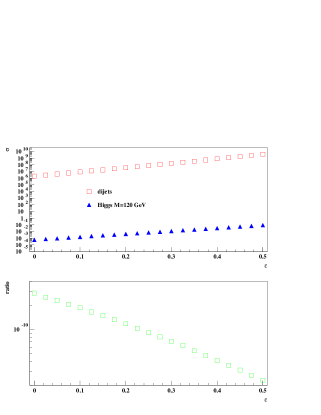
Figure 13: Higgs boson and dijet production at Tevatron: raw cross-sections and their ratio for different values of $\epsilon$, at $M_{H}=120{\rm GeV}$.

Figure 14: Differential dijet cross-sections for different values of $\epsilon$, compared to a reference taken at $\epsilon=0.08$. All cross-sections are normalised to the same value. The values $\epsilon=0.08$, 0.2 and 0.5 correspond, respectively, to the soft, hard (measurement at HERA), and hard BFKL pomeron intercepts.

Figure 15: Raw cross-sections vs. $\epsilon$

Figure 16: Higgs compared to dijets and diphotons as a function of $\epsilon$

Fig. 14 shows the $\epsilon$-dependence of the differential dijet cross-section $d\sigma_{JJ}/dM_{JJ}$, when compared to ($i.e.$, divided by) a reference distribution, taken at $\epsilon=0.08$. A strong dependence is found, meaning that the study of this distribution, independently from its normalisation, should allow to constrain the value of $\epsilon$, and to obtain a more precise prediction for the Higgs boson cross-section at the LHC Similar studies can be done with dilepton and diphoton events, which will benefit from much central mass resolution.

In Fig. 16 we give the cross-sections for dijets, $b\bar{b}$, $\gamma\gamma$, and Higgs boson, and in Fig. 16, the ratio of the Higgs cross-section with respect to $\gamma\gamma$ and $b\bar{b}$ as a function of $\epsilon$ for the LHC. Namely, it will allow to get a prediction on these cross-sections, once $\epsilon$ been determined, e.g. at the Tevatron.

These last remarks highlight once more the interest of DPE diphoton and dilepton production. Indeed, the experimental resolution on photon, electron and muon momenta is much better than the jet energy resolution, since in this case the events benefit from tracking information and/or electromagnetic calorimetry with a much better defined energy scale. Moreover, especially in the dilepton case, the hard sub-process is essentially quark-initiated (see formula (6)), and the knowledge of $Q_{P}$ is much more precise than that of $G_{P}$, thus eliminating another source of uncertainty. The measurement of $\epsilon$ will also be possible using the diphoton and dilepton measurement and the dependence of the cross-sections as a function the diphoton or the dilepton mass.

5.4 Predictions: summary and comparison

In Table 6, we give, where available, the cross-sections obtained by the different models. The factorizable numbers at the LHC (second column) should contain a factor accounting for the unknown rapidity gap survival probability (denoted $SP$); this factor is around 0.1 at the Tevatron. The numbers from the proton-induced model refer to $exclusive$ production, and are as such not refering to strictly the same process as the pomeron induced ones. The various models have fundamentally different philosophies and assumptions, so that caution should be taken not to conclude from any numerical agreement that the models themselves agree.

process and cuts	(1)	(2)	(3)	(4)
Higgs, 115 GeV, Tev	1.7	0.029-0.092	0.03	0.00012
Higgs, 115 GeV, LHC	169.	379.-486. $\times SP$	1.4	0.19
Higgs, 160 GeV, LHC	123.	145. $\times SP$	0.55	-
$\gamma\gamma$, Tev, $E_{T}>12GeV$, $\eta<2$	71.	128. (27.)	-	$\sim$ 20.
$\gamma\gamma$, Tev, $E_{T}>12GeV$, $\eta<1$	9.	8. (2.)	-	-
$\gamma\gamma$, LHC, $E_{T}>50GeV$, $\eta<2$	1.5	-	-	0.1
$\gamma\gamma$, LHC, $E_{T}>120GeV$, $\eta<5$	19.	-	0.12	-

Table 6: DPE Higgs and diphoton production cross-section at the LHC and the Tevatron (fb) for different models. (1): non factorisable pomeron based model (present work), (2): factorisable pomeron based model (the results contain both the pomeron and the reggeon components. For the $\gamma\gamma$ cross-section, we give in parenthesis the contribution of the pomeron only). (3): proton based model (exclusive case; the results are given for a Higgs mass of 120 GeV), (4): soft color interaction models.

6 Advantage of diffractive vs. “standard” Higgs boson production

As is now well-known [1, 2, 3] [22]-a, exclusive DPE events are very attractive from the experimental point of view, since the measurement of the outgoing protons momenta, using dedicated forward detectors (like roman pots or microchambers [21]) allows to determine the mass of the centrally produced system with excellent precision, so that the Higgs boson signal can be extracted from the DPE continuum background. Moreover, the background itself is strongly suppressed due to angular momentum conservation constraints (the “$J_{Z}=0$” rule [8], see section 2.1). Exclusive DPE events are however not an experimentally established process according to the data currently at our disposal. As we have emphazised, the “quasi-exclusive processes” which are quite close in topology from the exclusive processes are established processes and may keep an essential part of the nice kinematical features of the exclusive production.

In general inclusive DPE events, the angular momentum constraint above does not apply and the background is not suppressed, so that the a priori signal-to-background ratio ($S/B$) is similar to that of “standard” non-diffractive events. The missing mass method will not work as such, since the equality between the missing mass to the outgoing protons and the mass of the central system does not hold.

However, inclusive DPE events can still be kinematically constrained in a much stronger way than non-diffractive events. If, in addition to the forward proton detectors, the experiments can dispose of very forward calorimetry (e.g. up to $\eta\sim 8$, as was proposed in [25]), one may use the measurement of the Pomeron remnants to fully constrain the events kinematics. Combined with the higher cross-sections predicted in this last case, it shows that such forward calorimetry would be adapted and necessary. The first resolutions using these detectors are given in [6].

The idea is to use the forward calorimeters as vetos. The central mass is reconstructed with the proton momenta only, and events are considered only if the measured remnant energy is small enough. In a sense, this is a way to select “quasi-exclusive” events. Fig. 3 of Ref. [6] shows the achievable resolution as a function of the remnant veto.

Let us finish this discussion with an important point concerning the interest of the $\tau\tau$ decay mode. According to section 3, the inclusive DPE $\tau\tau$ cross-section is very small compared to the DPE dijet cross-section, and this is understood from the smallness of the QED coupling constant and the quark component of the Pomeron. Compared to this, the Higgs boson branching fraction into $\tau$ pairs is still $\sim 10\%$ in the mass range we consider. It follows from the cross-sections given earlier (see Table 3, and Fig. 10) that the cross-section ratio for $\tau$-pair events is ${\cal O}(10)$ at for example $m_{\tau\tau}\sim 130$  GeV for inclusive DPE events, whereas this mode is invisible through non-diffractive events.

Of course, the missing energy in $\tau$ decays, the presence of the Z peak in the $\tau$-pair cross-section, and other background processes not considered here spoil these numbers to some extent, but we do consider that this channel needs investigation. Also note that a pseudoscalar Higgs boson A, which appears in models with an extended Higgs sector (such as the supersymmetric models), does not couple to gauge bosons and hence preserves a significant branching fraction into $\tau$-pairs up to very high masses, where the effect of the Z peak is negligible; the same remark is true for the MSSM h boson in some regions of the parameter space.

7 Summary

The present work is meant to serve as a reference to the non factorizable, Pomeron induced DPE model.

• The original exclusive DPE formulation are recalled, and the inclusive expressions are introduced, see formulae (4-7).

• A systematic study is performed, that sheds light on the rôle of the various model parameters. It is emphasized that the forthcoming Tevatron data will allow to constrain their values, and answer the pending question of the existence of exclusive DPE production.

• Precise predictions for discovery physics at the LHC will then be possible; we focused on the Higgs boson case.

• It is recalled that, assuming favourable exprimental installations, the $b\bar{b}$ decay mode of the Higgs boson may well be exploited in double diffractive production.

• On the theoretical side, the H$\rightarrow\tau\tau$ channel is most promising, although some experimental difficulties have to be overcome.

Appendix

The cross-sections for the hard processes that are used in our study are summarized below, in terms of the usual Mandelstam variables. For dijet production, we take:

$$\frac{d\sigma_{gg\rightarrow qq}}{dt}=\frac{\pi\alpha_{S}^{2}}{s^{2}}\left(\frac{1}{6}\frac{u^{2}+t^{2}}{ut}-\frac{3}{8}\frac{u^{2}+t^{2}}{s^{2}}\right)$$ (9)

$$\frac{d\sigma_{gg\rightarrow gg}}{dt}=\frac{\pi\alpha_{S}^{2}}{s^{2}}\frac{9}{2}\left(3-\frac{ut}{s^{2}}-\frac{us}{t^{2}}-\frac{st}{u^{2}}\right)$$ (10)

For dilepton production, we have:

$$\frac{d\sigma_{qq\rightarrow ll}}{dt}=\frac{\pi\alpha^{2}}{s^{2}}\frac{4}{3}\frac{u^{2}+t^{2}}{s^{2}}C_{EW}$$ (11)

Here $C_{EW}$ includes electromagnetic and weak factors accounting for photon and Z exchange between the initial quark pair and the final leptons. Its expression is, for a quark of flavour $i$:

$$C_{EW}=e_{i}^{2}-e_{i}\frac{s(s-M_{Z}^{2})(L_{e}+R_{e})(L_{q}+R_{q})}{8x_{W}(1-x_{W})[(s-M_{Z}^{2})^{2}+M_{Z}^{2}\Gamma_{Z}^{2}]}+\frac{s^{2}(L_{e}^{2}+R_{e}^{2})(L_{q}^{2}+R_{q}^{2})}{64x_{W}^{2}(1-x_{W})^{2}[(s-M_{Z}^{2})^{2}+M_{Z}^{2}\Gamma_{Z}^{2}]}$$ (12)

Above, $x_{W}$ is the weak mixing angle, $M_{Z}$ and $\Gamma_{Z}$ are the Z boson mass and width, and L and R are the left and righthanded chiral couplings. Finally, the diphoton production cross-section reads:

$$\frac{d\sigma_{qq\rightarrow\gamma\gamma}}{dt}=\frac{\pi\alpha^{2}}{s^{2}}e_{i}^{4}\frac{1}{3}\left(\frac{u}{t}+\frac{t}{u}\right)$$ (13)

$$\frac{d\sigma_{gg\rightarrow\gamma\gamma}}{dt}=\frac{\alpha^{2}\alpha_{S}^{2}}{8\pi s^{2}}\left(\sum_{i}e_{i}^{2}\right)\frac{1}{8}C_{loop}$$ (14)

where $C_{loop}$ is a complicated expression resulting from the loop integral occurring in the $gg\rightarrow\gamma\gamma$ process. Its detailed expression can be found in [18].

References

- [1] A. Bialas and P. V. Landshoff, Phys. Lett. B256 (1990) 540; A. Bialas and W. Szeremeta, Phys. Lett. B296 (1992) 191; A. Bialas and R. Janik, Zeit. für. Phys. C62 (1994) 487.
- [2] J. D. Bjorken, Phys. Rev. D47 (1993). For a complete list, see also: A. Schafer, O. Nachtmann and R. Schöpf, Phys. Lett. B249 (1990) 331; J.-R. Cudell and O. F. Hernandez, Nucl. Phys. B471 (1996) 471; H. J. Lu, J. Milana Phys. Rev. D51 (1995) 6107; D. Graudenz, G. Veneziano Phys. Lett. B365 (1996) 302; M. Heyssler, Z. Kunszt, W.J. Stirling, Phys. Lett. B406 (1997) 95; E. M. Levin, hep-ph/9912403 and references therein; V. A. Khoze, A. D. Martin and M. G. Ryskin, Eur. Phys. J. C14 (2000) 525, id. C19 (2001) 477, hep-ph/0006005; V. A. Khoze, hep-ph/0105224.
- [3] M. G. Albrow and A. Rostovtsev, hep-ph/0009336.
- [4] M. Boonekamp, R. Peschanski and C. Royon, Phys. Rev. Lett. 87 (2001) 251806.
- [5] CDF Collab., T. Affolder et al., Phys. Rev. Lett. 85 (2000) 5043.
- [6] M. Boonekamp, A. De Roeck, R. Peschanski and C. Royon, hep-ph/0205332, Phys. Lett. B550 (2002) 93.
- [7] P. V. Landshoff, O. Nachtmann, Zeit. für. Phys. C35 (1987) 405;
-
[8]
J. Pumplin, Phys. Rev. D52 (1995) 1477;
A. Berera, J. C. Collins, Nucl. Phys. B474 (1996) 183. - [9] See V. A. Khoze, in [2].
- [10] A. Donnachie, P. V. Landshoff, Phys. Lett. B207 (1988) 319.
- [11] H1 Collab., C. Adloff et al., Z. Phys. C76 (1997) 613.
-
[12]
P. Laycock, talk given at 10th Intl. Workshop on Deep
Inelastic Scattering (DIS 2002), Cracow, May 2002 Acta Phys.Polon. B33 (2002) 3413;
F. P. Schilling idem, hep-ex/0209001, Acta Phys.Polon. B33 (2002) 3419;
P. R. Newman, Talk at low-x Meeting, Antwerpen, September 2002. - [13] CDF Collab., T. Affolder et al., Phys. Rev. Lett. 84 (2000) 4215.
- [14] C. Royon, L. Schoeffel, J. Bartels, H. Jung, R. Peschanski, Phys. Rev. D63 (2001) 074004.
- [15] B. L. Combridge and C. J. Maxwell, Nucl. Phys. B239 (1984) 429.
- [16] B. L. Combridge J. Kripfganz, J. Ranft, Phys. Lett. B70 (1977) 234.
- [17] E. Eichten, I. Hinchliffe, K. D. Lane, C. Quigg, Rev. Mod. Phys.56 (1984) 579; , Addendum-ibid. 58 (1986)1065.
- [18] E. L. Berger, E. Braaten, R. D. Field, Nucl. Phys. B239 (1984) 52.
- [19] SHW, see www.physics.rutgers.edu/jconway/soft/shw/shw.html.
- [20] L. Schoeffel, Acta. Phys. Polon. B33 (2002) 3425.
- [21] R. Orava, talk at LISHEP02, Rio de Janeiro, February 2002.
-
[22]
-a V. A. Khoze, A. D. Martin, M. G. Ryskin,
Eur.Phys.J. C24 (2002) 581;
-b B. Cox, J. Forshaw, B. Heinemann, Phys. Lett.; B540 (2002) 263, R. B. Appleby, J. R. Forshaw, Phys. Lett. B541 (2002) 108;
-c R. Enberg, G. Ingelman, A. Kissavos, N. Timneanu, Phys. Rev. Lett. 89 (2002) 081801, R. Enberg, G. Ingelman, N. Timneanu, Phys. Rev. D67 (2003) 011301, with references to the two versions (SCI and GAL) of the model. - [23] B. E. Cox, J. R. Forshaw, Comput. Phys. Commun. 144 (2002) 104.
- [24] T. Sjostrand, P. Eden (Nordita), C. Friberg, L. Lonnblad, G. Miu, S. Mrenna, E. Norrbin, Comput. Phys. Commun. 135 (2001) 238.
- [25] CMS Collab., Technical Design Report (1997).