Equation of State of Oscillating Brans-Dicke Scalar and Extra Dimensions

Abstract

We consider a Brans-Dicke scalar field stabilized by a general power law potential with power index $n$ at a finite equilibrium value. Redshifting matter induces oscillations of the scalar field around its equilibrium due to the scalar field coupling to the trace of the energy momentum tensor. If the stabilizing potential is sufficiently steep these high frequency oscillations are consistent with observational and experimental constraints for arbitrary value of the Brans-Dicke parameter $\omega$. We study analytically and numerically the equation of state of these high frequency oscillations in terms of the parameters $\omega$ and $n$ and find the corresponding evolution of the universe scale factor. We find that the equation of state parameter can be negative and less than -1 but it is not related to the evolution of the scale factor in the usual way. Nevertheless, accelerating expansion is found for a certain parameter range. Our analysis applies also to oscillations of the size of extra dimensions (the radion field) around an equilibrium value. This duality between self-coupled Brans-Dicke and radion dynamics is applicable for $\omega=-1+1/D$ where D is the number of extra dimensions.

I Introduction

Observations of the magnitude-redshift relation of distant Type Ia supernovaeRiess:1998cb and CMB measurementsdeBernardis:2001xk have indicated that the universe is undergoing a period of accelerated expansion. Attributing this acceleration to a cosmological constant is not completely satisfactory (see e.g. Sahni:1999gb ) because fine tuned initial conditions are required in order to solve the coincidence problem (why the vacuum energy is dominating the energy density right now). Thus, acceleration is attributed to the influence of a redshifting non-luminus form of energy with negative pressure called by many authors ‘dark energy’ or ‘quintessence’Peebles:1987ek . The origin of this form of energy remains unknown. Several types of scalar fieldsPeebles:1987ek have been proposed as sources of dark energy including the dilaton, the inflaton, supersymmetric partners of fermions, Brans-Dicke (hereafter BD) scalarsBrans:sx , etc.

The dynamical evolution of these scalars is determined by specially designed potentials so that the scalar field energy density tracks the radiation-matter component at early times while at late times it dominates and leads to acceleration. The main drawback of these models is that there is usually no physical motivation for the proposed scalar fields and potentials.

Cosmological theories with extra dimensions generically contain a scalar field of geometrical origin which describes the size of extra dimensions. This is known as the radion field. These theories have the potential of providing a physically motivated solution to the hierarchy problem by postulating that the fundamental Planck mass $M_{*}$ is close to the $TeV$ scale Antoniadis:1990ew ; pap.Dim ; Randall:1999vf . This is possible in theories with extra dimensions pap.Dim because Gauss’s law relates the Planck scales of the $4+D$-dimensional theory $M_{*}$ and the long distance $4$-dimensional theory $M_{pl}$ by

$$M_{pl}^{2}=b_{0}^{D}M_{*}^{D+2}$$ (1)

where $b_{0}$ is the present stabilized size of the extra dimensions.

According to observations, the internal space should be static or nearly static at least from the time of primordial nucleosynthesisGZ(CQG2) . This means that at the present evolutionary stage of the Universe only small fluctuations over stabilized or slowly varying compactification scales (conformal scales/geometrical moduli) are possible. Thus the size of the extra dimensions $b(t)$ (the radion field) is usually assumed to be stabilized to its present value $b_{0}$ by a ‘radion stabilizing potential’ $V(b)$. Observational constrains require this stabilization and theoretical modelsGoldberger:1999uk have been proposed to justify it. Within the framework of multidimensional cosmological models the role of the size of extra dimensions as a stabilized scalar field with possible excited states was investigated in GZ1 ; GZ ; GZ(PRD2) where they were called gravitational excitons.

In a recent paperPerivolaropoulos:2002pn we demonstrated that a generic feature of these theories is the existence of radion oscillations (induced by redshifting matter density) around the equilibrium value $b_{0}$ at the minimum of the stabilizing potential. It was also shown that these oscillations can lead to cosmological periods of accelerating expansion of the universe. However the radion mass required for such extremely low frequency oscillations was too small (at the classical level) to be consistent with fifth force experimental constraintsWill:2001mx ; Steinhardt:1994vs . In the same paperPerivolaropoulos:2002pn it was also demonstrated that the dynamics of the radion field are formally equivalent with the dynamics of a massive BD scalar with $\omega=-1+1/D$ where $D$ is the number of extra dimensions (see also Cline:2002mw ; Levin:yw ).

Quintessence models based on BD scalars (extended quintessence) have the theoretically appealing property that the same scalar field that participates in the gravity sector is enhanced by a potentialSantos:1996jc to play the role of quintessence. Even though no oscillating BD scalars have been studied so far, there is an extensive literature on extended quintessenceTorres:2002pe ; Faraoni:2001tq ; Perrotta:1999am .

Here we focus on the cosmological evolution of high frequency oscillationsAccetta:yb ; Steinhardt:1994vs of a BD scalarBrans:sx (or equivalently a radion field) stabilized by an arbitrary power law potential. For large enough frequencies $\nu\buildrel>\over{\sim}10^{12}Hz$ these oscillations are consistent with fifth force constraintsAccetta:yb ; Steinhardt:1994vs and they can play the role of dark matter and/or dark energy for a wide range of parameters.

The structure of this paper is the following: In section II we review the cosmological evolution of an oscillating minimally coupled scalar field. In section III we demonstrate the equivalence between radion dynamics in $D$ extra dimensions and massive BD scalar $\phi$ with $\omega=-1+1/D$, $\phi=b^{2D}$ and focus on the dynamics of an oscillating BD scalar. We derive a virial theorem that connects the kinetic and potential energies of the oscillating field in terms of the parameters $\omega$ and $n$. This theorem is verified by numerically solving the dynamical cosmological field equations for various parameter values. We then use this virial theorem to find the equation of state that connects the effective pressure with the effective energy density of the oscillating field. In section IV we use the equation of state to find the redshift rate of the effective energy density and the evolution of the cosmological scale factor. We find that the energy redshift and the scale factor evolution are independent of $\omega$ and depend only on the stabilizing potential power index $n$. The validity of these results is demonstrated numerically. Finally in section V we conclude and discuss possible extensions and open issues related to this work. In what follows we set $8\pi G=1$.

II Minimally Coupled Oscillating Scalar

As a warm up exercise we evaluate the equation of state for a minimally coupled coherently oscillating scalar in an expanding background. This analysis was originally done in Ref. Turner:1983he but we briefly review it here for completeness and for comparison of the results with the BD scalar oscillations analysis performed in the following sections.

Consider a minimally coupled scalar field whose dynamics is determined by the Lagrangian density

$${\cal L}={1\over 2}\partial_{\mu}\phi\partial^{\mu}\phi-V(\phi)$$ (2)

Assuming a Robertson-Walker metric we obtain the field equation

$$\ddot{\phi}+3H\dot{\phi}=-\frac{dV}{d\phi},$$ (3)

where $H={{\dot{a}}\over a}$. From the energy momentum tensor we obtain the energy density $\rho$ and the pressure $p$ as

$$\rho = {1\over 2}{\dot{\phi}}^{2}+V(\phi)$$ (4)

$$p = {1\over 2}{\dot{\phi}}^{2}-V(\phi)$$ (5)

Using equations (3) and (4) we obtain

$${d\over{dt}}\rho=-3H\dot{\phi}^{2}$$ (6)

We now consider a potential of the form

$$V(\phi)=\lambda|\phi|^{n}$$ (7)

where $n>0$ and focus on oscillations of the scalar field around its minimum. We also define the mean value of a time dependent quantity $q(t)$ as

$${\bar{q}}\equiv{1\over T}\int_{0}^{T}dt\;q(t)$$ (8)

where T is the period of one oscillation. The mean equation of state of the oscillating field is

$$\bar{p}=w\bar{\rho}$$ (9)

We now evaluate the equation of state parameter $w$ in terms of $n$.

Using equations (4), (5), (6) and (9) we obtain

$${{d\bar{\rho}}\over{dt}}=-3H\bar{\dot{\phi^{2}}}=-3H\gamma\bar{\rho}=-3{{\dot{a}}\over a}\gamma\bar{\rho}$$ (10)

where $\gamma=w+1$ and we have assumed $T\ll H^{-1}$. Thus, on timescales $\Delta t\ll H^{-1}$ we have ${{\Delta\bar{\rho}}\over{\bar{\rho}}}\ll 1$ and we can set

$$\rho={1\over 2}{\dot{\phi}}^{2}+V(\phi)\simeq V(\phi_{max})\equiv V_{max}=\bar{\rho}$$ (11)

where $\phi_{max}$ is the amplitude of the $\phi$ oscillations and $V_{max}$ is the corresponding maximum potential energy. We now have

$$\gamma={{\bar{p}+\bar{\rho}}\over{\bar{\rho}}}={{\bar{\dot{\phi^{2}}}}\over{\bar{\rho}}}={\sqrt{2}\over T_{max}}\int_{0}^{T_{max}}{{d\phi}\over V_{max}^{1/2}}(1-V/V_{max})^{1/2}$$ (12)

We also use equation (11) to find the time $T_{max}={T\over 4}$ it takes the field to go from 0 to $\phi_{max}$

$$T_{max}={1\over{\sqrt{2}\;V_{max}^{1/2}}}\int_{0}^{\phi_{max}}d\phi(1-V/V_{max})^{-1/2}$$ (13)

Using equations (12) and (13) we find

$$\gamma=2{{\int_{0}^{\phi_{max}}d\phi(1-V/V_{max})^{1/2}}\over{\int_{0}^{\phi_{max}}d\phi(1-V/V_{max})^{-1/2}}}={{2n}\over{n+2}}$$ (14)

where we made use of (7).

The energy density redshift is now obtained from equation (10) as

$$\rho=\rho_{0}\left({a\over a_{0}}\right)^{-3\gamma}$$ (15)

Using this equation and the Friedman equation

$${{\dot{a}}\over a}^{2}={\rho\over 3}$$ (16)

we obtain

$$a\sim t^{2/3\gamma}=t^{{n+2}\over{3n}}$$ (17)

and accelerated expansion is obtained in the range $0<n<1$. The cosmological effects of this accelerated expansion for an oscillating minimally coupled scalar have been discussed in Ref. Sahni:1999qe . The scalar field evolution for power index $n$ in the above range is well defined even though for $n<1$, $V^{\prime}(\phi)$ is weakly singular at $\phi=0$. $V(\phi)$ can be made mathematically more appealing by the field redefinition $\phi\rightarrow(\phi^{2}+\phi_{c}^{2})^{1/2}$, $\phi_{c}\rightarrow 0$ which does not change the above resultsSahni:1999qe . In the next section we will show that even though the equation of state is different for an oscillating BD scalar, accelerated expansion is obtained for the same range of the power index $n$.

III Virial Theorem and Equation of State for Oscillating Radion and Brans-Dicke Scalar

In this section we demonstrate the equivalence between BD and Radion dynamics (for specific values of the BD parameter $\omega$) and then focus on the BD theory to derive a virial theorem and the equation of state of the scalar field oscillations.

Consider the BD action

$${\cal S}=\frac{1}{2}\int d^{4}x\sqrt{-g}\left[\phi R-{\omega\over{\phi}}\partial_{\mu}\phi\partial^{\mu}\phi-2V(\phi)\right]+L_{fluid}$$ (18)

where $L_{fluid}$ describes matter and/or radiation. We assume a flat ($k=0$) Friedmann-Robertson-Walker model whose metric reads

$$ds^{2}=-dt^{2}+a^{2}(t)[dr^{2}+r^{2}d\theta^{2}+r^{2}\sin^{2}\theta d\phi^{2}]$$ (19)

The combination of equations (18) and (19) leads to the dynamical equations for $\phi$ and $a$

$${\dot{a}^{2}\over{a^{2}}}+{\dot{a}\over{a}}{\dot{\phi}\over{\phi}}-{\omega\over{6}}{\dot{\phi}^{2}\over{\phi^{2}}}-{V\over{3\phi}}={\rho\over{3\phi}},$$ (20)

$$2{\ddot{a}\over{a}}+{\dot{a}^{2}\over{a^{2}}}+{\ddot{\phi}\over{\phi}}+2{\dot{a}\over{a}}{\dot{\phi}\over{\phi}}+{\omega\over{2}}{\dot{\phi}^{2}\over{\phi^{2}}}-{V\over{\phi}}=-{p\over{\phi}},$$ (21)

$${\ddot{\phi}}+3{\dot{a}\over{a}}{\dot{\phi}}={(\rho-3p)\over{2\omega+3}}+{2\over{2\omega+3}}\left[2V-\phi{dV\over{d\phi}}\right]$$ (22)

From the field equations we can read the effective energy and pressure (see e.g. Sen:2000vj ; Torres:2002pe ) for the field which end up being,

$$\rho_{\phi}={\omega\over{2}}~{}{\dot{\phi}^{2}\over{\phi}}+V-3{\dot{a}\over{a}}\dot{\phi}$$ (23)

and

$$p_{\phi}={\omega\over{2}}~{}{\dot{\phi}^{2}\over{\phi}}-{V}+\ddot{\phi}+2{\dot{a}\over{a}}\dot{\phi}$$ (24)

The BD theory is interesting in its own right as a generalization of Einstein gravity. In addition however many physically motivated theories reduce to BD gravity for specific values of $\omega$. For example the superstring dilaton is akin to a BD theory with $\omega=-1$. Also Einstein gravity generalized to 4+D dimensions reduces to an effective 4-dimensional BD theory with $\omega=-1+1/D$. This can be demonstrated as follows:

We consider a 3-brane embedded in a toroidally compact ($4+D$) dimensional space-time $R^{1}\times R^{3}\times T^{D}$ with the $D$ extra spatial dimensions (the bulk) stabilized at a size $b_{0}$. The total action may be written as

$$S_{tot}=S_{bulk}+S_{brane}$$ (25)

where

$$S_{bulk}=\int d^{4+D}x\sqrt{-g{{}^{(4+D)}}}\biggl{(}\frac{1}{16\pi\overline{G}}{\cal{R}}[g]+{\cal L_{\rm bulk}}\biggr{)}$$ (26)

and

$$S_{brane}=\int d^{4}x\sqrt{-g{{}^{(4)}}}\;{\cal L_{\rm brane}}$$ (27)

In (26) ${\cal L_{\rm bulk}}$ is the Lagrangian of the bulk fields apart from the graviton. These fields give rise to the stabilizing potential $V$ discussed below. The background metric for the a toroidally compact ($4+D$) dimensional space-time which is consistent with the symmetries of the brane-bulk system may be written as

$$g_{MN}=diag[1,-a^{2}(t)\tilde{g}_{ij},-b^{2}(t)\tilde{g}_{mn}]$$ (28)

where $M,N$ run from 0 to $D+3$; $i,j$ run from $1$ to 3 and $m,n$ run from 4 to $D+3$. Also $a(t)$ is the scale of the non-compact 3-dimensional flat space (the scale factor of the universe) and $b(t)$ is the radius of the compactified toroidal space (the radion field).

We assume that matter on the brane ($S_{brane}$) is represented by a classically conserved perfect fluid energy momentum tensor $T_{\mu\nu}=(\rho+p)u_{\mu}u_{\nu}+pg_{\mu\nu}$ ($\mu,\;\nu=0,...,3$) with $\nabla_{\mu}T^{\mu\nu}=0$ where $u_{\mu}$ is a future-oriented time-like vector $u^{\mu}=(1,\vec{0}_{3+D})$ in the basis (28) and $\rho$ is the energy density of the brane matter. Also $p=w\rho$ is the corresponding pressure. We also include a radion stabilizing potential

$$V(b)\equiv b(t)^{D}\int d^{4+D}x\;{\cal L_{\rm bulk}}$$ (29)

induced by some non-specified bulk dynamics ${\cal L_{\rm bulk}}$Goldberger:1999uk . For example a uniform bulk cosmological constant is represented by $V=b^{D}\Lambda$ while a Casimir type potential would be $V(b)=kb^{-4}$ Gardner:2001fz . We assume that bulk dynamics lead to a potential $V(b)$ that stabilizes $b$ at

$$b_{0}=\left({M_{Pl}^{2}\over M_{*}^{D+2}}\right)^{1/D}$$ (30)

with a vanishing cosmological constant. The equations of motion for the coupled $(a(t),b(t))$ system can be written asArkani-Hamed:1999gq

$$6\frac{\dot{a}^{2}}{a^{2}}+D(D-1)\frac{\dot{b}^{2}}{b^{2}}+6D\frac{\dot{a}}{a}\frac{\dot{b}}{b}=2\frac{V+\rho}{b^{D}}$$

$$\frac{\ddot{b}}{b}+(D-1)\frac{\dot{b}^{2}}{b^{2}}+3\frac{\dot{a}}{a}\frac{\dot{b}}{b}=2\frac{1}{b^{D}}\left(\frac{2V}{D+2}-\frac{b}{D(D+2)}\frac{\partial V}{\partial b}+\frac{\rho-3p}{2(D+2)}\right)$$ (31)

$$\frac{\ddot{a}}{a}+2\frac{\dot{a}^{2}}{a^{2}}+D\frac{\dot{a}}{a}\frac{\dot{b}}{b}=2\frac{1}{b^{D}}\left(\frac{b}{2(D+2)}\frac{\partial V}{\partial b}-\frac{D-2}{2(D+2)}V+\frac{\rho+(D-1)p}{2(D+2)}\right)$$

In the picture of Refs. pap.Dim (see also Arkani-Hamed:1999gq ) (ADD) and Randall:1999vf (RS), the matter-radiation energy density is assumed to be localized on the brane corresponding to the $a(t)$ scale factor. This localized energy density in general distorts the geometry of the compactified $D$-dimensional space (the bulk), but as far as the overall properties and the evolution of the radion are concerned, it is correct to treat the energy density on the wall as just being averaged over the whole space as done on the RHS of these equations. This assumption is consistent with the results of references Csaki:1999mp ; Csaki:1999jh where it was shown that the coupling of the radion field to the energy momentum tensor is given generically through the trace $(\rho-3p)$ plus terms involving the stabilizing potential $V(b)$.

Equations (III) have been analyzed in the context of inflation (away from the stabilization point $b_{0}$) in Arkani-Hamed:1999gq (ADD model).

Similar equations Csaki:1999mp arise in the context of Randall-Sundrum (RS) models Randall:1999vf , where the hierarchy problem is solved using extra dimensions of smaller sizes at the expense of introducing a non-flat background metric along the extra coordinates and a pair of branes whose distance $b(t)$ is stabilized at $b_{0}$ by the potential $V(b)$.

From equations (III) it is clear that radiation $(p_{rad}={1\over 3}\rho_{rad})$ has no effect on the dynamics of the radion. This is not the case however for matter. Redshifting matter plays the role of a driving force and can induce radion oscillations during both the matter and radiation eras. These oscillations backreact on the scale factor $a(t)$ through the effective Friedman equations (III) and can affect the expansion rate.

It is interesting to compare the form of the cosmological equations (III) with the non-conventional cosmology on the brane of Ref. Binetruy:1999ut which has shown that terms of $O(\rho^{2})$ appear on the Friedman equation due to the extra dimensions. These terms can also be obtained from the system (III) in the limit $({{\dot{b}}\over b})^{2}\ll\rho$. In that limit, it is a good approximation to set ${\dot{b}}=0$ in the second of equations (III). For a stabilizing potential of the form $V\sim(b-b_{0})^{n}$ we thus obtain $V\sim\rho^{{n\over{n-1}}}$ and for a standard parabolic potential ($n=2$) we obtain an extra $\rho^{2}$ contribution due to the potential in the first equation of the system (III) similar to the $\rho^{2}$ terms of Ref. Binetruy:1999ut . For a generalized stabilizing potential the extra term in the Friedman equation is of the form $\rho^{\alpha}$ ($\alpha={n\over{n-1}}$) and can provide a physical motivation for Cardassian expansionFreese:2002sq . In what follows however we will not use the above approximation which ignores the effects of radion oscillations and we will focus on the cosmological expansion induced by these oscillations for a generalized stabilizing potential.

It is straightforward to show that we can obtain the set of dynamical equations (III) for the radion by setting to the corresponding BD set of equations (20), (21), (22)

$$\phi = b^{D}$$

$$\omega = -1+{1\over D}$$

Thus the radion dynamics is equivalent to BD dynamics for particular values of $\omega$. Even though our study will be based on the general BD field equations (20), (21) and (22) the main physical application of our results will be $4+D$ dimensional Einstein gravity for which $\omega=-1+1/D$. Even though these values of $\omega$ are of $O(1)$ they are consistent with experimental and observational constraints because of the presence of the potential $V$. This stabilizing potential can confine the effects of any modifications of Newton’s law to scales smaller than $1mm$ Accetta:yb ; Steinhardt:1994vs ; Perivolaropoulos:2002pn . On these scales there are no firm experimental constraints on the form of the gravitational potentialWill:2001mx .

We now consider the BD field equations (20), (21), (22) with a potential $V(\phi)$ having a minimum at $\phi_{0}$. It is clear from equation (22) that even if we consider an initially static field $\phi=\phi_{0}$ the redshifting matter will induce small oscillations around the equilibrium position (approximately $\phi_{0}$) by slowly shifting the equilibrium position of the field $\phi$. We will thus study the equation of state of the energy density of these small oscillations assuming a potential of the form

$$V(\phi)=\lambda|\phi-\phi_{0}|^{n}\equiv\lambda|\delta\phi|^{n}$$ (32)

Since not all three equations of the system (20), (21) and (22) are independent (because of the Bianchi identities) we focus on (20) and (22) and write them in dimensionless form as

$${\dot{a}^{2}\over{a^{2}}}+{\dot{a}\over{a}}{\dot{\phi}\over{\phi}}-{\omega\over{6}}{\dot{\phi}^{2}\over{\phi^{2}}}={1\over{\phi}}({1\over{a^{3}}}+\bar{\rho_{v}}|\phi-1|^{n})$$ (33)

$${\ddot{\phi}}+3{\dot{a}\over{a}}{\dot{\phi}}={3\over{(2\omega+3)}}({1\over{a^{3}}}+4\bar{\rho_{v}}|\phi-1|^{n}\mp 2n\phi\bar{\rho_{v}}|\phi-1|^{n-1})$$ (34)

where we have assumed the presence of matter redshifting like

$$\rho_{m}(t)=\rho_{0m}({{a_{0}}\over{a(t)}})^{3}$$ (35)

(radiation has no effect on the evolution of $\phi$ since $\rho_{r}-3p_{r}=0$). We have also set $a_{0}\equiv a(t_{p})=1$ where $t_{p}$ is the present time) and

$${\rho_{0m}\over 3}t \longrightarrow t$$ (36)

$${\phi\over\phi_{0}} \longrightarrow \phi$$ (37)

$${{\lambda\phi_{0}^{n}}\over\rho_{0m}} \longrightarrow \bar{\rho_{v}}$$ (38)

The $-$ sign ($+$ sign) in equation (34) is valid when $\phi>1$ ($\phi<1$). As in the case of the minimally coupled scalar of section II $\phi$ is periodic on timescales $\Delta t<<H^{-1}$. With no loss of generality we may therefore focus on the half period $T\over 2$ for which $\delta\phi\equiv\phi-1>0$. We also assume $\delta\phi\ll 1$. Thus equation (34) is written as

$$\ddot{\delta\phi}+{{6n\bar{\rho_{v}}}\over{2\omega+3}}\delta\phi^{n-1}={3\over{2\omega+3}}{1\over a^{3}}-3{\dot{a}\over{a}}\dot{\delta\phi}$$ (39)

This implies that

$${d\over{dt}}({{\dot{\delta\phi^{2}}}\over 2}+{{6\bar{\rho_{v}}}\over{2\omega+3}}\delta\phi^{n}-{3\over{2\omega+3}}{1\over a^{3}}\delta\phi)=-3{\dot{a}\over{a}}\dot{\delta\phi^{2}}$$ (40)

Therefore the effective potential that determines the dynamics of the oscillating BD scalar is

$$V^{eff}(\phi)={{6\bar{\rho_{v}}}\over{2\omega+3}}\delta\phi^{n}-{3\over{2\omega+3}}{1\over a^{3}}\delta\phi$$ (41)

For $n>1$ the effective potential is not minimized at $\delta\phi=0$ but at the time-dependent value

$$\delta\phi_{eql}=({3\over{6n\bar{\rho_{v}}}}{1\over a^{3}})^{1\over{n-1}}$$ (42)

If the amplitude of oscillations $\delta\phi_{max}$ is much larger than the shift of equilibrium point due to matter redshift then we may ignore the shift and assume that the oscillations take place around $\delta\phi=0$. In the opposite case when $\delta\phi_{eql}\gg\delta\phi_{max}$ we may ignore the oscillations and assume that $\delta\phi\simeq\delta\phi_{eql}$ at all times. In the later case the energy density of the BD scalar is dominated by potential energy V which redshifts like

$$V(\phi)\sim a^{-3n/(n-1)}$$ (43)

and is therefore subdominant compared to matter at late times. Thus in what follows we focus on the former case assuming

$$\delta\phi_{max}\gg\delta\phi_{eql}$$ (44)

It will be shown that for $n<4$ this condition is an attractor in the sense that even if it is not realized at early times it becomes true at late times i.e. $\delta\phi_{max}$ redshifts slower than $\delta\phi_{eql}$. Thus since the oscillations of $\delta\phi$ take place symmetrically around $\delta\phi=0$ and since the period and amplitude are approximately constant on timescales much less than $H^{-1}$ the mean value of $\delta\phi$ (and of $\dot{\delta\phi}$) vanishes and equation (40) implies

$${{\bar{\dot{\delta\phi^{2}}}}\over 2}+{{6\bar{\rho_{v}}}\over{2\omega+3}}\bar{\delta\phi^{n}}\simeq{{6\bar{\rho_{v}}}\over{2\omega+3}}\delta\phi_{max}^{n}\equiv V_{max}^{eff}$$ (45)

Proceeding in similar way as in the previous section (equations (10) - (14)) we have

$$\bar{\dot{\delta\phi^{2}}}=2V_{max}^{eff}{{\int_{0}^{\delta\phi_{max}}d\delta\phi(1-V^{eff}/V_{max}^{eff})^{1/2}}\over{\int_{0}^{\delta\phi_{max}}d\delta\phi(1-V^{eff}/V_{max}^{eff})^{-1/2}}}=V_{max}^{eff}{{2n}\over{n+2}}$$ (46)

Using now this result and equations (41), (45) we find

$$\bar{V}^{eff}=V_{max}^{eff}(1-{n\over{n+2}})={2\over{n+2}}V_{max}^{eff}$$ (47)

and

$${{\bar{\dot{\delta\phi^{2}}}}\over\bar{V^{eff}}}=n\Rightarrow{{\bar{\dot{\delta\phi^{2}}}}\over{\bar{\rho_{v}}\bar{\delta\phi^{n}}}}={{6n}\over{2\omega+3}}$$ (48)

This result is a virial theorem for BD scalar oscillations connecting the mean kinetic and potential energies. We have numerically confirmed the validity of this theorem by solving the full system (33), (34) for $\bar{\rho_{v}}\gg 1$ (high frequency oscillations) from $t_{i}={1\over\sqrt{\bar{\rho_{v}}}}$ to $t_{0}=1$. We used initial conditions

$$\dot{\delta\phi}(t_{i}) = 0$$ (49)

$$\delta\phi(t_{i}) = \delta\phi_{max}\ll 1$$ (50)

$$a(t_{i}) = (2/3)^{-2/3}t_{i}^{-2/3}$$ (51)

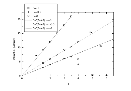
Figure 1: The virial ratio ${{\bar{\dot{\delta\phi^{2}}}}\over{\bar{\rho_{v}}\bar{\delta\phi^{n}}}}$ as a function of $n$ for three values of $\omega$ ($\omega=0$ lower line, $\omega=-0.5$, and $\omega=-1$ upper line). Notice that the virial theorem (straight lines) is violated for $n\buildrel>\over{\sim}4$

In Figure 1 we show the virial ratio ${{\bar{\dot{\delta\phi^{2}}}}\over{\bar{\rho_{v}}\bar{\delta\phi^{n}}}}$ as a function of $n$ for three values of $\omega$. The points correspond to numerically obtained values while the lines are the corresponding analytical results (48). For $n<4$ the analytically obtained results are well verified by the numerics. For $n\geq 4$ however the agreement is not good and the virial ratio rapidly drops instead of increasing. This domination of the potential energy is due to the violation of the condition (44). The evolution of $\phi$ for $n=6$ shown in Figure 2 indicates that the oscillations of $\delta\phi$ do not even overlap with $\delta\phi=0$ and therefore the assumption $\bar{\delta\phi}=0$ used in deriving the virial theorem is not realized for $n\geq 4$. This may be understood by comparing the redshift rate of

$${\delta\phi}_{min}\sim a^{-3/(n-1)}$$ (52)

(cf equation (42)) with that of

$${\delta\phi}_{max}\sim a^{-6/(n+2)}$$ (53)

which will be derived in the next section (see equation (63)). It is easy to see that for $n<4$, ${\delta\phi}_{max}$ eventually dominates while for $n>4$ it is ${\delta\phi}_{min}$ that dominates leading to violation of the virial theorem and vanishing of the virial ratio since the potential energy dominates.

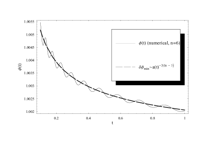
Figure 2: The oscillations of $\delta\phi$ do not even overlap with $\delta\phi=0$ for $n=6$. The equilibrium value ${\delta\phi}_{min}$ is larger than the oscillation amplitude ${\delta\phi}_{max}$ and redshifts like $a^{-3/5}\sim t^{-2/5}$ (matter energy dominated in the evolution). Thus the assumptions of the virial theorem are violated.

The fact that the oscillations of $\phi(t)$ are effectively around $\phi=1$ for $n<4$ is demonstrated in Figure 3 which shows the evolution of $\phi(t)$ for $n=1.5$. The oscillation amplitude ${\delta\phi}_{max}$ redshifts like $a^{-6/(n+2)}$ as predicted analytically (see equation (63)).

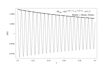
Figure 3: For $n=1.5$ the BD scalar oscillations are approximately symmetric around $\phi\simeq 1$ ($\omega=0$ was used in the evolution but the result was found to be independent of $\omega$)

The period of the oscillations varies slowly with time and it can be calculated using equation (45) in a similar way as for a minimally coupled scalar (equation (13)). The result is that the oscillation period $T$ redshifts like

$$T\sim a^{{3(n-2)}\over{n+2}}$$ (54)

i.e. it decreases for $n<2$ while it increases for $n>2$. This result is confirmed numerically in Figure 4 where we show $ln({{T(a)}\over{T(a=1)}})$ vs $ln(a)$. The numerically obtained points are in good agreement with the analytically predicted corresponding lines for $n=1.5$ (decreasing T), $n=2$ (constant T) and $n=3.0$ (increasing T).

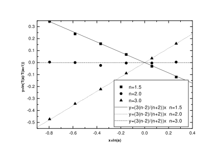
Figure 4: The oscillation period increases (decreases) for $n>2$ ($n<2$).

We are now in position to calculate the equation of state that connects the mean effective pressure with the mean effective energy density of the BD oscillating field. Using the rescaling of equations (36)-(38) and equations (23), (24) we find that for small approximately symmetric oscillations

$$\bar{\rho}_{\phi} \simeq {\omega\over 6}\bar{\dot{\delta\phi^{2}}}+\bar{\rho}_{v}\bar{\delta\phi^{n}}$$ (55)

$$\bar{p}_{\phi} \simeq {\omega\over 6}\bar{\dot{\delta\phi^{2}}}-\bar{\rho}_{v}\bar{\delta\phi^{n}}$$ (56)

Thus keeping the notation of section II we have

$$\gamma={{\bar{\rho}_{\phi}+\bar{p}_{\phi}}\over{\bar{\rho}_{\phi}}}={{{\omega\over 3}\bar{\dot{\delta\phi^{2}}}}\over{\bar{\rho}_{\phi}}}$$ (57)

Using now equations (46) - (48) we find

$$\gamma={{2\omega n}\over{\omega n+2\omega+3}}=w+1$$ (58)

or

$$w={{\omega n-(2\omega+3)}\over{\omega n+(2\omega+3)}}$$ (59)

For a minimally coupled scalar this result would immediately imply that the redshift of the energy density is of the form of equation (15) with $\gamma$ given by (58). If that were the case, superaccelerationTorres:2002pe ; Faraoni:2001tq ($\dot{H}>0$ which may be favored observationallyCaldwell:1999ew ) would be easily obtained for negative values of $\omega$ which lead to $w<-1$ (see Figure 5). For a BD scalar however this is not the case. It is easily seen by using e.g. equation (40) that the continuity equation

$$\dot{\bar{\rho_{\phi}}}+3{\dot{a}\over a}({\bar{\rho}_{\phi}+\bar{p}_{\phi}})=0$$ (60)

is not realizedTorres:2002pe for $\bar{\rho}_{\phi}$ and $\bar{p}_{\phi}$.

Figure 5: The equation of state parameter $w$ is less than $-1$ for negative $\omega$.

Therefore $\bar{\rho}_{\phi}$ does not redshift like $a^{-3\gamma}$. The redshift rate of the effective energy density and the corresponding evolution of the scale factor $a(t)$ are studied in the next section.

IV Energy Redshift and Scale Factor Evolution

Even though the continuity equation (60) is not realized for a BD scalar, equation (40) can be used to derive the effective energy density redshift. For symmetric oscillations this equation implies

$${d\over{dt}}({{\bar{\dot{\delta\phi^{2}}}}\over 2}+{{6\bar{\rho_{v}}}\over{2\omega+3}}\bar{\delta\phi^{n}})=-3{\dot{a}\over{a}}\bar{\dot{\delta\phi^{2}}}$$ (61)

Using now equations (45) and (46) we find

$${d\over{dt}}V_{max}^{eff}=-6{\dot{a}\over{a}}V_{max}^{eff}{n\over{n+2}}$$ (62)

which implies

$$V_{max}^{eff}\sim a^{-{{6n}\over{n+2}}}\sim\delta\phi_{max}^{n}$$ (63)

and leads to equation (53) used in the previous section. Using now equations (55), (46), (47) and (63) we find

$$\bar{\rho}_{\phi}\sim V_{max}^{eff}\sim a^{-{{6n}\over{n+2}}}$$ (64)

which gives the redshift rate of the BD energy density. It is interesting to note that even though the equation of state parameter $w$ differs from that of a minimally coupled scalar and depends on $\omega$, the redshift rate of the energy density is independent of $\omega$ and is similar to the corresponding result of a minimally coupled scalar. This result is numerically verified in Figure 6 where we show a plot of $-ln(\rho_{\phi}(a)/\rho_{\phi}(a=1))$ vs $ln(a)$ obtained numerically for various values of the scale factor $a$ and for three values of $n$ ($n=1.5$, $n=2.0$ and $n=3$). According to equation (64), the numerically obtained points should lie on straight lines with slope $3\Gamma$ where

$$\Gamma={{2n}\over{n+2}}$$ (65)

This is indeed realized as shown in Figure 6 where we also show these straight lines.

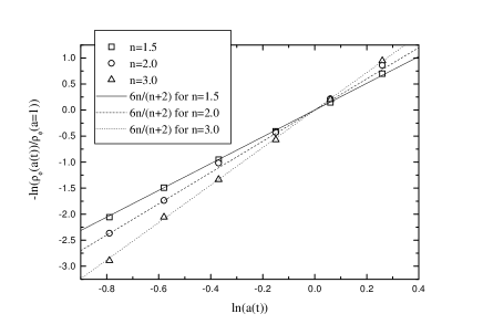
Figure 6: The energy density of the oscillating BD scalar redshifts according to the analytical predictions for three values of $n$.

We now focus on the evolution of the scale factor in the presence of an oscillating BD scalar given the above derived energy density redshift. To isolate the effects of the scalar we ignore the presence of matter at this stage. Thus the rescaled Friedman equation (33) is approximated by

$${\dot{a}^{2}\over{a^{2}}}\simeq{\omega\over{6}}\bar{\dot{\delta\phi^{2}}}+\bar{\rho_{v}}\bar{\delta\phi^{n}}\simeq Ba^{-3\Gamma}$$ (66)

where B is a constant and $\Gamma$ determines the redshift rate of $\bar{\rho_{\phi}}$ and is given by equation (65). This implies that

$$a\sim t^{{2\over{3\Gamma}}}\sim t^{{n+2}\over{3n}}$$ (67)

Thus even though $\gamma\neq\Gamma$ in the case of a BD scalar oscillations, the induced scale factor evolution is identical to that of a minimally coupled scalar shown in equation (17). This result is numerically verified in Figure 7 where we show a plot of $ln({{a(t)}\over{a_{0}}})$ vs $ln({t\over t_{0}})$ (we chose $t_{0}\simeq 2/3$ and $a_{0}=a(t_{0})$). The dark continous line corresponds to the numerical scale factor evolution for $n=1.5$ while the light dashed line is the corresponding analytical result of equation (67).

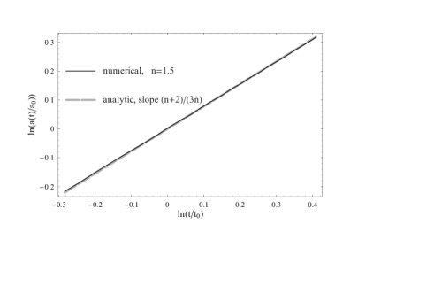
Figure 7: The numerically obtained evolution of the scale factor is in good agreement with the analytical prediction for $n=1.5$ when matter is not present.

The agreement is quite good, confirming the analytical expectation. It is interesting to note that this result implies accelerated expansion for $0<n<1$ as in the case of a minimally coupled scalar. The oscillations in this case however can be generically induced not just by initial conditions but also by the time dependent redshift of the minimum $\delta\phi_{eql}$ of the effective potential (41).

The scale factor evolution derived above when matter is not present can be combined with equation (53) to find the time evolution of $\delta\phi_{max}$. The predicted power law $\delta\phi_{max}\sim t^{2/n}$ is verified numerically in Figure 8 for $n=1.5$.

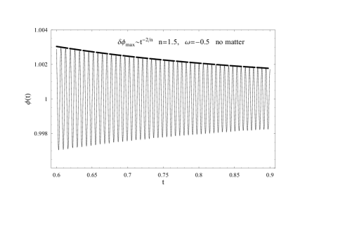
Figure 8: The numerically obtained evolution of the $\delta\phi_{max}$ is in good agreement with the analytical prediction $\delta\phi_{max}\sim t^{2/n}$for $n=1.5$.

V Radion Oscillations - Outlook

The above derived results can easily be applied to the case of radion dynamics. By setting $\omega=-1+1/D$ in equation (59) we can obtain the equation of state parameter for high frequency radion oscillations in terms of the number of extra dimensions $D$ as

$$w={{n(D-1)+(D+2)}\over{n(D-1)-(D+2)}}$$ (68)

Clearly $w$ is negative and in fact less than $-1$ for a wide range of parameters $n$, $D$. The evolution of the scale factor however is independent of $D$ and is given by equation (67). This result is in agreement with Ref. Perivolaropoulos:2002pn where the case $n=2$ was studied.

Even though radion oscillations can not lead to superacceleration, they do lead to accelerating expansion for $n<1$ as in the case of a minimally coupled scalar field. Thus, the mechanism of Ref. Sahni:1999qe of quintessence from an oscillating minimally coupled scalar with $n<1$ can be extended to the case of an oscillating BD scalar and in particular the case of an oscillating radion. In fact an oscillating radion has two potential advantages over an oscillating minimally coupled scalar. First its origin is better defined and better motivated since it is a generic geometrical prediction of theories with extra dimensions. Second, as discussed below, tracking can in principle be achieved at early times by the coupling to the matter energy momentum tensor which generically induces radion oscillations due to the matter redshift (the effective potential is time dependent). Since this possibility does not exist for a minimally coupled scalar, an exponential potential has to be usedSahni:1999qe for large $\phi$ so that the energy density in $\phi$ tracks the matter component at early times while at late times the field oscillates around its potential minimum with $n<1$ thus producing the observed accelerated evolution of the scale factor. The potential used in Ref. Sahni:1999qe that combines an exponential behavior at large $\phi$ with power law behavior with power index $n$ around its minimum is

$$V(\phi)=V_{0}(cosh\;\lambda\phi-1)^{n/2}$$ (69)

Our results on the scale factor evolution indicate that the analysis of Ref. Sahni:1999qe is applicable to the case of radion oscillations even though the equation of state is different in the case of the radion. However, the coupling of the radion to the trace of the matter energy momentum tensor opens up a new possibility for achieving tracking at early times. The radion could start very close to its effective potential $\delta\phi_{eql}$ minimum at early times with subdominant oscillations ($\delta\phi_{max}\ll\delta\phi_{eql}$) induced by the time dependent shift of the minimum of the effective potential (41). The radion energy during this early evolution can track the matter energy density. At late times when $\delta\phi_{max}>\delta\phi_{eql}$ the oscillations can dominate and lead to accelerating expansion for $n<1$. This mechanism has the possible advantage of avoiding the introduction of a tuned potential. Instead only the existence of a stabilizing potential minimum is required and a power law behavior around it. The viability of this type of mechanism is an interesting problem worth of further investigation.

A possible direct observational signature of radion oscillations is the existence of a coherent high frequency gravitational wave background. Even though the frequency of these gravitational waves is expected to be of order $10^{12}Hz$ and is much beyond the range of current experiments, a detailed study of their features could be interesting. A study of gravitational wave backgrounds from extra dimensions induced by other mechanisms can be found in Ref. Hogan:2000is .

The stability of the field configurations against spatial fluctuations is also an interesting issue. Homogeneous oscillating scalar fields have been shown to fragment into baryons (Affleck-Dine mechanismAffleck:1984fy ), Q-Balls Kasuya:1999wu or I-Balls Kasuya:2002zs depending on their potential and number of components. Since the oscillating radion corresponds to a real scalar field it may be possible to fragment into a generalization of I-Balls (BD I-Balls) with interesting cosmological consequences.

Acknowledgements: I thank G. Leontaris, I. Rizos and T. Vachaspati for useful discussions. This work was supported by the European Research and Training Network HPRN-CT-2000-00152.

References

- (1) A. G. Riess et al. [Supernova Search Team Collaboration], Astron. J. 116, 1009 (1998) [arXiv:astro-ph/9805201]; S. Perlmutter et al. [Supernova Cosmology Project Collaboration], Astrophys. J. 517, 565 (1999) [arXiv:astro-ph/9812133].
- (2) P. de Bernardis et al., Astrophys. J. 564, 559 (2002) [arXiv:astro-ph/0105296].
- (3) V. Sahni and A. A. Starobinsky, Int. J. Mod. Phys. D 9, 373 (2000) [arXiv:astro-ph/9904398].
- (4) P. J. Peebles and B. Ratra, Astrophys. J. 325, L17 (1988); R. R. Caldwell, R. Dave and P. J. Steinhardt, Phys. Rev. Lett. 80, 1582 (1998) [arXiv:astro-ph/9708069];I. Zlatev, L. M. Wang and P. J. Steinhardt, Phys. Rev. Lett. 82, 896 (1999).
- (5) C. Brans and . H. Dicke, Phys. Rev. 124, 925 (1961).
- (6) I. Antoniadis, Phys. Lett. B 246 (1990) 377.
- (7) N. Arkani-Hamed, S. Dimopoulos and G. Dvali, Phys. Lett. B 429(1998) 263 [hep-ph/9803315], Phys. Rev.D 59 (1999) 086004 [hep-ph/9807344]; I. Antoniadis, N. Arkani-Hamed, S. Dimopoulos and G. R. Dvali, Phys. Lett. B 436 (1998) 257 [arXiv:hep-ph/9804398].
- (8) L. Randall and R. Sundrum, Phys. Rev. Lett. 83, 4690 (1999) [arXiv:hep-th/9906064]; Phys. Rev. Lett. 83, 3370 (1999) [arXiv:hep-ph/9905221].
- (9) U. Günther and A. Zhuk, Class. Quant. Grav. 18, (2001), 1441 - 1460, hep-ph/0006283.
- (10) W. D. Goldberger and M. B. Wise, Phys. Rev. Lett. 83, 4922 (1999) [arXiv:hep-ph/9907447].
- (11) U. Günther and A. Zhuk, Phys. Rev. D56, (1997), 6391 - 6402, gr-qc/9706050.
-
(12)
U. Günther and A. Zhuk, Stable compactification and
gravitational excitons from extra dimensions, (Proc. Workshop
”Modern Modified Theories of Gravitation and Cosmology”, Beer
Sheva, Israel, June 29 - 30, 1997), Hadronic Journal 21, (1998),
279 - 318, gr-qc/9710086;
U. Günther, S. Kriskiv and A. Zhuk, Gravitation & Cosmology 4, (1998), 1 -16, gr-qc/9801013;
U. Günther and A. Zhuk, Class. Quant. Grav. 15, (1998), 2025 - 2035, gr-qc/9804018. - (13) U. Günther and A. Zhuk, Phys. Rev. D61, (2000), 124001, hep-ph/0002009.
- (14) L. Perivolaropoulos and C. Sourdis, Phys. Rev. D 66, 084018 (2002) [arXiv:hep-ph/0204155].
- (15) C. M. Will, Living Rev. Rel. 4, 4 (2001) [arXiv:gr-qc/0103036].
- (16) P. J. Steinhardt and C. M. Will, Phys. Rev. D 52, 628 (1995) [arXiv:astro-ph/9409041].
- (17) J. M. Cline and J. Vinet, arXiv:hep-ph/0211284.
- (18) J. J. Levin, Phys. Lett. B 343, 69 (1995) [arXiv:gr-qc/9411041].
- (19) C. Santos and R. Gregory, Annals Phys. 258, 111 (1997) [arXiv:gr-qc/9611065].
- (20) D. F. Torres, Phys. Rev. D 66, 043522 (2002) [arXiv:astro-ph/0204504].
- (21) V. Faraoni, Int. J. Mod. Phys. D 11, 471 (2002) [arXiv:astro-ph/0110067].
- (22) F. Perrotta, C. Baccigalupi and S. Matarrese, Phys. Rev. D 61, 023507 (2000) [arXiv:astro-ph/9906066];A. Riazuelo and J. P. Uzan, Phys. Rev. D 66, 023525 (2002) [arXiv:astro-ph/0107386];G. Esposito-Farese and D. Polarski, Phys. Rev. D 63, 063504 (2001) [arXiv:gr-qc/0009034].
- (23) F. S. Accetta and P. J. Steinhardt, Phys. Rev. Lett. 67, 298 (1991); J. McDonald, Phys. Rev. D 44, 2325 (1991) [Erratum-ibid. D 45, 1433 (1991)]; Phys. Rev. D 48 (1993) 2462.
- (24) M. S. Turner, Phys. Rev. D 28, 1243 (1983).
- (25) V. Sahni and L. M. Wang, Phys. Rev. D 62, 103517 (2000) [arXiv:astro-ph/9910097].
- (26) S. Sen and T. R. Seshadri, arXiv:gr-qc/0007079.
- (27) C. L. Gardner, Phys. Lett. B 524, 21 (2002) [arXiv:hep-th/0105295].
- (28) N. Arkani-Hamed, S. Dimopoulos, N. Kaloper and J. March-Russell, Nucl. Phys. B 567, 189 (2000) [arXiv:hep-ph/9903224]; J. M. Cline, Phys. Rev. D 61, 023513 (2000) [arXiv:hep-ph/9904495].
- (29) C. Csaki, M. Graesser, C. Kolda and J. Terning, Phys. Lett. B 462, 34 (1999) [arXiv:hep-ph/9906513];
- (30) C. Csaki, M. Graesser, L. Randall and J. Terning, Phys. Rev. D 62, 045015 (2000) [arXiv:hep-ph/9911406]; P. Kanti, I. I. Kogan, K. A. Olive and M. Pospelov, Phys. Rev. D 61 106004 (2000) [arXiv:hep-ph/9912266].
- (31) P. Binetruy, C. Deffayet and D. Langlois, Nucl. Phys. B 565, 269 (2000) [arXiv:hep-th/9905012].
- (32) K. Freese and M. Lewis, Phys. Lett. B 540 1 (2002) [arXiv:astro-ph/0201229].
- (33) R. R. Caldwell, Phys. Lett. B 545, 23 (2002) [arXiv:astro-ph/9908168].
- (34) C. J. Hogan, Phys. Rev. Lett. 85, 2044 (2000) [arXiv:astro-ph/0005044].
- (35) I. Affleck and M. Dine, Nucl. Phys. B 249, 361 (1985).
- (36) S. Kasuya and M. Kawasaki, Phys. Rev. D 61, 041301 (2000) [arXiv:hep-ph/9909509].
- (37) S. Kasuya, M. Kawasaki and F. Takahashi, arXiv:hep-ph/0209358.