The form factor of the pion in “point-form” of relativistic dynamics revisited

Abstract

The electromagnetic form factor of the pion is calculated in the “point-form” of relativistic quantum mechanics using simple, phenomenological wave functions. It is found that the squared charge radius of the pion is predicted one order of magnitude larger than the experimental value and the asymptotic behavior expected from QCD cannot be reproduced. The origin of these discrepancies is analyzed. The present results confirm previous ones obtained from a theoretical model and call for major improvements in the implementation of the “point-form” approach.

I Introduction

The pion charge form factor has been the object of many studies Isgur:1984jm ; Chung:1988mu ; Cardarelli:1995dc ; Roberts:1996hh ; Choi:1997iq ; deMelo:1997cb ; Maris:2000sk ; Krutov:2002nu ; Allen:1998hb . The simplicity of the system, a quark – anti-quark bound state, and the availability of experimental data Bebek:1978pe ; Amendolia:1986wj ; Volmer:2000ek make it very attractive to test both physical ingredients and methods employed in its calculation. In view of a strongly bound system (if one assumes constituent quark masses of the order of a few hundred MeV) and the large $Q^{2}$ at which the pion form factor has been measured, a relativistic calculation is most likely required. There are various approaches to implement relativity, ranging from field theory to relativistic quantum mechanics. Among the latter ones, calculations of the pion form factor have been done in instant and front forms Isgur:1984jm ; Chung:1988mu ; Cardarelli:1995dc ; Roberts:1996hh ; Choi:1997iq ; deMelo:1997cb ; Maris:2000sk ; Krutov:2002nu . Only one has been performed in the less known “point-form” Klink:1998 . A good agreement with experiment was claimed by the authors Allen:1998hb .

In this “point-form” approach the parameter determining the elastic form factor is the relative velocity of the initial and final states. Thus, in the Breit frame, the form factor depends on the momentum transfer $Q^{2}$ only through the quantity, $v^{2}=Q^{2}/(4\,M^{2}+Q^{2})$, where $M$ is the total mass of the system. This has the immediate consequence that the squared charge radius of the system scales like $1/M^{2}$, and therefore tends to $\infty$ when $M$ goes to zero. Accordingly, the charge radius increases when the system becomes stronger bound, contrary to physical intuition. For the pion, this argument suggests that the squared charge radius should be of the order of $3/(2\,M_{\pi}^{2})\simeq 3\,{\rm fm}^{2}$, which exceeds the experimental value by almost one order of magnitude. In contrast to this result, the calculation of Ref. Allen:1998hb shows nice agreement. Furthermore, these authors show that, in the case of an infinitely bound system, the form factor could scale like $1/Q^{2}$ for large momentum transfers, in agreement with the QCD expectation Brodsky:1975vy ; Lepage:1979zb . However, the general derivation of this result does not imply any assumption on the binding of the system.

Motivated by the above observations, we re-examine in this letter the “point-form” calculation of the pion form factor. While doing so, we also have in mind the failure of the approach when applied to a system made of scalar constituents Desplanques:2001zw ; Amghar:2002jx . The main goal of this study is a clarification of the above-mentioned peculiarities connected with recent implementations of the “point-form” of relativistic Hamiltonian mechanics. A deeper understanding of this relatively unknown approach should certify that the method is on a safe ground. With this aim we will use simple wave functions (a Gaussian one as used in Ref. Allen:1998hb and a Hulthén one), which allow analytic calculations, providing a better insight on some of the features that the approach evidences.

II Expressions of form factors in “point-form”

The expression of the pion form factor can be defined quite generally as:

$$\sqrt{2E_{f}\;2E_{i}}\;\left<f|J^{\mu}|i\right>=F_{1}(q^{2})\,(P^{\mu}_{f}+P^{\mu}_{i}).$$ (1)

By identifying the matrix element of the current with its expression in terms of wave functions, an expression for the form factor $F_{1}(q^{2})$ can be obtained. We first remind below results obtained for spin-0 constituents and then present expressions for the spin-1/2 case.

II.1 Spin-0 constituent case

The matrix element relative to the “point-form” form factor for a system of spin-less particles may be written:

$$\sqrt{2E_{f}\,2E_{i}}\;\left<f|J^{\mu}|i\right>=\sqrt{2M_{f}\,2M_{i}}\;\frac{1}{(2\pi)^{3}}\int d^{4}p\,d^{4}p_{f}\,d^{4}p_{i}\,d\eta_{f}\,d\eta_{i}\,\theta(\lambda_{f}\cdot p_{f})\;\theta(\lambda_{f}\cdot p)\;\theta(\lambda_{i}\cdot p)\;\theta(\lambda_{i}\cdot p_{i})$$ (2)

$$\times\delta(p^{2}-m^{2})\;\delta(p^{2}_{f}-m^{2})\;\delta(p^{2}_{i}-m^{2})\;\delta^{4}(p_{f}+p-\lambda_{f}\eta_{f})\;\delta^{4}(p_{i}+p-\lambda_{i}\eta_{i})\;\phi_{f}\left((\frac{p_{f}-p}{2})^{2}\right)\;\phi_{i}\left((\frac{p_{i}-p}{2})^{2}\right)$$

$$\hskip 142.26378pt\times\left[\sqrt{(p_{f}+p)^{2}\,(p_{i}+p)^{2}}\;\;\;(p_{f}^{\mu}+p_{i}^{\mu})\right].$$

Notations have been explained in Ref. Desplanques:2001zw . Let us mention here that the four-vectors $\lambda$ represent the velocities of the system in the initial and final states, $\lambda^{\mu}_{i,f}=P^{\mu}_{i,f}/M$.

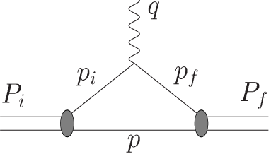
Figure 1: Graphical representation of a virtual photon absorption on a pion together with kinematical definitions.

The kinematics is otherwise given in Fig. 1. The $\eta$ variables have been introduced to make the covariance explicit. After performing some of the integrals, the matrix element of the current may be written:

$$\sqrt{2E_{f}\,2E_{i}}\;\left<f|J^{\mu}|i\right> = \sqrt{2M_{f}\,2M_{i}}\;\frac{1}{(2\pi)^{3}}\int\frac{d\vec{p}}{2\,e_{p}}\;\frac{\phi_{f}\left((\frac{p_{f}-p}{2})^{2}\right)\;\phi_{i}\left((\frac{p_{i}-p}{2})^{2}\right)}{(2\,\lambda_{i}\cdot p_{i})\;(2\,\lambda_{f}\cdot p_{f})}$$ (3)

$$\qquad\times\left[\sqrt{(p_{f}+p)^{2}\,(p_{i}+p)^{2}}\;\;\;(p_{f}^{\mu}+p_{i}^{\mu})\right].$$

In this expression, it is understood that the arguments $p_{i}^{\mu}$ and $p_{f}^{\mu}$ must be replaced by their value that stem from the $\delta(\cdots)$ functions appearing in Eq. (2), which after integrating over the $\eta$ variables imply:

$$\vec{p}_{i}+\vec{p}=\frac{\vec{P}_{i}}{E_{i}}\;(e_{i}+e_{p}),\qquad\qquad\vec{p}_{f}+\vec{p}=\frac{\vec{P}_{f}}{E_{f}}\;(e_{f}+e_{p}).$$ (4)

These relations characterize boost transformations in the “point-form” implementation proposed in Ref. Klink:1998 . They differ from those used in instant- or front-form approaches.

In the Breit frame, the above expressions allow one to write the form factor, $F_{1}(q^{2})$, as:

$$F_{1}(q^{2})=\frac{1+v^{2}}{\sqrt{1-v^{2}}}\int\frac{d\vec{p}}{(2\pi)^{3}}\;\phi_{f}(\vec{p}_{tf})\;\phi_{i}(\vec{p}_{ti}),$$ (5)

where $Q^{2}=-q^{2}$, $v^{2}=Q^{2}/(4\,M^{2}_{\pi}+Q^{2})$ and $\vec{p}_{ti,f}^{\,2}=p_{x}^{2}+p_{y}^{2}+(p_{z}\pm v\,e_{p})^{2}/(1-v^{2})$. It can be checked that this last expression of the form factor, or Eq. (3) after an appropriate change of variable, leads to the relation:

$$F_{1}(0)=\int\frac{d\vec{k}}{(2\pi)^{3}}\;\phi^{2}(\vec{k})=1,$$ (6)

in complete agreement with the charge of the system on the one hand, the ortho-normalization of the solutions of a mass operator on the other hand (no extra k-dependent factor is introduced in the integrand).

The expression of Eq. (2) may not be unique however. Due to the somewhat arbitrary appearance of the mass term, $M$, at the r.h.s., which should come out dynamically, an improved expression was proposed in Ref. Amghar:2002jx . Apart from the fact that it does not allow one to get analytic formulas, it does not add anything to the present discussion.

II.2 Spin-1/2 constituent case

In order to calculate the pion form factor, one has to take into account the spinorial properties of the constituent quarks as well as the pseudo-scalar nature of the pion. A minimal covariant factor accounting for these features involves the following trace of $\gamma$ matrices:

$$I^{\mu} \equiv 4\;{\rm Tr}\left\{\gamma_{5}\;\frac{(m+\gamma\cdot p_{i})}{2}\;\gamma^{\mu}\,\frac{(m+\gamma\cdot p_{f})}{2}\;\gamma_{5}\;\frac{(m-\gamma\cdot p)}{2}\right\}$$ (7)

$$= 2\;\left[p_{i}^{\mu}\;(p_{f}\cdot p)+p_{f}^{\mu}\;(p_{i}\cdot p)-p^{\mu}\;(p_{i}\cdot p_{f})+m^{2}\;(p_{i}^{\mu}+p_{f}^{\mu}+p^{\mu})\right].$$

At zero momentum transfer and when all particles are put on mass shell, this quantity becomes identical to $\sqrt{(p_{f}+p)^{2}\,(p_{i}+p)^{2}}\,(p_{f}^{\mu}+p_{i}^{\mu})$, which is just the factor that appears in the expression of the matrix element for scalar constituents, see Eq. (2). To get an expression for the pion form factor consistent with the normalization adopted for the solutions of the mass operator, it is therefore sufficient to replace this factor for scalar particles by the above expression $I^{\mu}$. One thus gets the following matrix element for the $J^{\mu}$ current:

$$\sqrt{2E_{f}\,2E_{i}}\;\left<f|J^{\mu}|i\right>=\sqrt{2M_{f}\,2M_{i}}\;\frac{1}{(2\pi)^{3}}\int d^{4}p\,d^{4}p_{f}\,d^{4}p_{i}\,d\eta_{f}\,d\eta_{i}\;\theta(\lambda_{f}\cdot p_{f})\;\theta(\lambda_{f}\cdot p)\;\theta(\lambda_{i}\cdot p)\;\theta(\lambda_{i}\cdot p_{i})$$ (8)

$$\times\;\delta(p^{2}-m^{2})\;\delta(p^{2}_{f}-m^{2})\;\delta(p^{2}_{i}-m^{2})\delta^{4}(p_{f}+p-\lambda_{f}\eta_{f})\;\delta^{4}(p_{i}+p-\lambda_{i}\eta_{i})\;\;\phi_{f}\left((\frac{p_{f}-p}{2})^{2}\right)\;\phi_{i}\left((\frac{p_{i}-p}{2})^{2}\right)$$

$$\qquad\qquad\times\,2\,\left[p_{i}^{\mu}\;(p_{f}\cdot p)+p_{f}^{\mu}\;(p_{i}\cdot p)-p^{\mu}\;(p_{i}\cdot p_{f})+m^{2}\;(p_{i}^{\mu}+p_{f}^{\mu}+p^{\mu})\right].$$

In the Breit frame, the matrix element of Eq. (8) leads to the expression for the form factor:

$$F_{1}(Q^{2})=\sqrt{1-v^{2}}\int\frac{d\vec{p}}{(2\pi)^{3}}\;\phi_{f}(\vec{p}_{tf})\;\phi_{i}(\vec{p}_{ti}).$$ (9)

It can be checked again that this last expression of the form factor is in complete agreement with the charge of the system and the ortho-normalization of the solutions of a mass operator.

It is noticed that the form factor of Eq. (9) differs from the one obtained with scalar constituent particles by a factor $(1-v^{2})/(1+v^{2})$, see Eq. (5). This last factor is close to $1-Q^{2}/(8\,m^{2})$ for small momentum transfers and small binding energies ($M\simeq 2\,m$). It may be identified with the Darwin-Foldy term sometimes introduced in the calculation of form factors involving spin-1/2 constituents. A similar factor can be found from Ref. Chung:1988mu as a result of Melosh rotations where, however, a quantity $2m$ appears in place of the pion mass $M_{\pi}$ in the definition of $v$.

III Analytic results for form factors

In a few cases, analytic expressions of form factors given by Eq. (9) can be obtained. This is the case for a Gaussian wave function, that has been used widely in the field (Refs. Isgur:1984jm ; Chung:1988mu ; Krutov:2002nu ; Allen:1998hb ), and a Hulthén one. The latter one is of interest because it leads to the correct asymptotic power law for the form factor in the case of scalar constituents. These wave functions with the appropriate normalizations are given by:

$$\phi^{G}(\vec{k})=\frac{(4\pi)^{3/4}}{b^{3/2}}\;\exp\left[-k^{2}/(2\,b^{2})\right],\qquad\qquad\phi^{H}(\vec{k})=\sqrt{4\,\pi}\;\frac{\sqrt{2\,\alpha\;\beta\;(\alpha+\beta)^{3}}}{(\alpha^{2}+k^{2})\;(\beta^{2}+k^{2})}.$$ (10)

The parameters may be chosen as free parameters or fitted to the matter radius. For the Hulthén wave function, $\alpha$ is in principle related to the binding energy by $\alpha^{2}=m^{2}-M^{2}/4$, only $\beta$ is really a free parameter. With these wave functions the integral in Eq. (9) may be calculated analytically. One gets in the Gaussian case:

$$F_{1}^{G}(Q^{2})=\sqrt{1-v^{2}}\;\int d\vec{p}\;\left(\frac{1}{b^{3/2}\;\pi^{3/4}}\right)^{2}\;\exp\left[-\frac{1}{b^{2}}\left(p^{2}_{\perp}+\frac{p^{2}_{\parallel}+v^{2}\;e^{2}_{p}}{1-v^{2}}\right)\right]=\frac{(1-v^{2})^{2}}{\sqrt{1+v^{2}}}\;\;\exp\left[-\frac{v^{2}}{1-v^{2}}\;\frac{m^{2}}{b^{2}}\right],$$ (11)

and the associated charge radius and asymptotic behavior are given by:

$$\left<r^{2}\right>^{G}\equiv-6\;\frac{dF_{1}^{G}(Q^{2})}{dQ^{2}}=\frac{6}{4\,M_{\pi}^{2}}\;\left(\frac{5}{2}+\frac{m^{2}}{b^{2}}\right),\qquad\left.F_{1}^{G}(Q^{2})\right|_{Q^{2}\rightarrow\infty}=\frac{1}{\sqrt{2}}\;\frac{16\,M_{\pi}^{4}}{Q^{4}}\;\;\exp\left[-\frac{Q^{2}}{16\,b^{2}}\;\frac{4\,m^{2}}{M_{\pi}^{2}}\right].$$ (12)

In the case of the Hulthén wave function, the form factor reads:

$$F_{1}^{H}(Q^{2}) = \sqrt{1-v^{2}}\,\int\frac{d\vec{p}}{(2\pi)^{3}}\;8\pi\alpha\beta\;(\alpha+\beta)^{3}$$ (13)

$$\times\frac{1}{\left(\alpha^{2}+p^{2}_{\perp}+(\frac{p_{\parallel}-v\,e_{p}}{\sqrt{1-v^{2}}})^{2}\right)\;\left(\beta^{2}+p^{2}_{\perp}+(\frac{p_{\parallel}-v\,e_{p}}{\sqrt{1-v^{2}}})^{2}\right)\left(\alpha^{2}+p^{2}_{\perp}+(\frac{p_{\parallel}+v\,e_{p}}{\sqrt{1-v^{2}}})^{2}\right)\;\left(\beta^{2}+p^{2}_{\perp}+(\frac{p_{\parallel}+v\,e_{p}}{\sqrt{1-v^{2}}})^{2}\right)}$$

$$= \frac{(1-v^{2})^{2}}{v}\;\;\frac{\alpha\;\beta\;(\alpha+\beta)}{(\alpha-\beta)^{2}}\left(\frac{\arctan[v\sqrt{m^{2}-\alpha^{2}}\,/\alpha]}{\sqrt{m^{2}-\alpha^{2}}}-\frac{{\rm arctan}[2\,v\sqrt{m^{2}-\alpha^{2}}\,/(\alpha+\beta-v^{2}(\beta-\alpha))]}{\sqrt{m^{2}-\alpha^{2}}}\right.$$

$$\qquad\qquad\left.+\,\frac{\arctan[v\,\sqrt{m^{2}-\beta^{2}}\,/\beta]}{\sqrt{m^{2}-\beta^{2}}}-\frac{{\rm arctan}[2\,v\sqrt{m^{2}-\beta^{2}}\,/(\alpha+\beta+v^{2}(\beta-\alpha))]}{\sqrt{m^{2}-\beta^{2}}}\right).$$

The charge radius and high $Q^{2}$ properties associated to this form factor are given by:

$$\left<r^{2}\right>^{H} = \frac{6}{4\,M_{\pi}^{2}}\;\left(2+\frac{\alpha\;(7\,\beta^{2}+4\,\beta\,\alpha+\alpha^{2})}{3\,\beta^{2}\;(\beta+\alpha)}+\frac{m^{2}-\alpha^{2}}{3}\;\frac{\beta^{4}+5\,\beta^{3}\,\alpha+12\,\beta^{2}\,\alpha^{2}+5\,\beta\,\alpha^{3}+\alpha^{4}}{\beta^{2}\,\alpha^{2}\;(\beta+\alpha)^{2}}\right)$$

$$\qquad\stackrel{{\scriptstyle\beta\rightarrow\infty}}{{\longrightarrow}}\frac{3}{M_{\pi}^{2}}+\frac{1}{8\,\alpha^{2}},$$

$$\left.F_{1}^{H}(Q^{2})\right|_{Q^{2}\rightarrow\infty} = \frac{64\,M_{\pi}^{8}\;\alpha\,\beta\;(\beta+\alpha)^{2}}{Q^{8}\;(m^{4}+\ldots)}\quad\stackrel{{\scriptstyle\beta\rightarrow\infty}}{{\longrightarrow}}\quad\frac{16\,M_{\pi}^{4}}{Q^{4}}\;\alpha\;\frac{\arctan[\sqrt{m^{2}-\alpha^{2}}\;/\alpha]}{\sqrt{m^{2}-\alpha^{2}}},$$ (14)

where the dots in the last expression represent contributions that can be neglected for finite values of $\beta$. An interesting limit is the Coulombian case $(\beta=\alpha)$, considered in Ref. Desplanques:2001zw for scalar constituents. The expressions in Eq. (14) then simplify to read:

$$\left<r^{2}\right>^{C}=\frac{6}{M_{\pi}^{2}}+\frac{3}{4\,\alpha^{2}},\qquad\qquad\left.F_{1}^{C}(Q^{2})\right|_{Q^{2}\rightarrow\infty}=\frac{256\,M_{\pi}^{8}\;\alpha^{4}}{Q^{8}\;m^{4}}.$$ (15)

IV Discussion

IV.1 Charge radius

As it can be observed from Eqs. (12) and (14), the squared charge radius scales like the inverse squared pion mass, confirming the hand-waving argument given in the introduction and, at the same time, the consequence that the charge radius increases with increasing binding energy!

The second observation is that the squared charge radius has a minimum value, as a function of the open parameters, that depends on the pion mass. It slightly differs with the model ($15/(4\,M_{\pi}^{2})$ for the Gaussian wave function and $3/M_{\pi}^{2}$ for the Hulthén one). However, even this minimal values, ($7.5\,{\rm fm}^{2}$ and $6\,{\rm fm}^{2}$) exceed by far the experimental one, $0.43\,{\rm fm}^{2}$ Amendolia:1986wj . Independently, the contribution of the bare matter radius of the pion to these values is not small. This part, $3/(8b^{2})$, is enhanced by $(2\,m/M_{\pi})^{2}$, which amounts to a factor $8$ - $18$ for quark masses in the range of $0.2$ - $0.3$ GeV. For a squared matter radius of $0.05\,{\rm fm}^{2}$, of the order of what is generally predicted by quark models, the corresponding squared charge radius is already of the order of the experimental one. The existence of a minimum value largely exceeding the experimental one has the striking consequence that there is no way to fit the parameters of the model to reproduce the experimental pion form factor.

IV.2 Asymptotic behavior

The asymptotic form factor for a system made of spin-1/2 constituents is expected to scale like $Q^{-2}$ Brodsky:1975vy ; Lepage:1979zb . In addition, the coefficient of the $Q^{-2}$ factor should be proportional to the strength of the short range quark-quark interaction (up to log terms) and to the square of the wave function at the origin. These expectations are independent of any assumption on the mass of the constituents or on the size of the system.

Evidently, the Gaussian model cannot reproduce the correct power law behavior of form factors in general. Only in the zero-size limit, when $b^{2}\rightarrow\infty$, one obtains $F_{1}\propto(M_{\pi}^{2}/Q^{2})^{2}$. Apart from the fact that the power of $Q$ is not the right one, the overall coefficient does not scale like the strength of the quark-quark interaction. This illustrates the statement that reproducing the QCD power-law behavior with Gaussian wave functions and standard currents is most surely the consequence of a mistake in the theoretical approach employed to get the result.

Not surprisingly, form factors calculated with Hulthén wave functions provide a power law behavior ($Q^{-8}$), which, however, differs from what is expected. For a large part, this is in relation with the observation made in Ref. Allen:2000ge that the transferred momentum to the struck particle in the “point-form” approach is $Q^{2}\;[1+Q^{2}/(4\,M^{2})]$ rather than $Q^{2}$. A better result is obtained in the limit $\beta\rightarrow\infty$, in which case the wave function, Eq. (10), scales like $k^{-2}$ instead of $k^{-4}$. This limit however corresponds to a zero-range force, which is difficult to imagine for an effect dominated by one-gluon exchange.

Apart from that, one can check that the expression of the form factor, Eq. (13), has at least some of the appropriate properties which can be easily checked in the Coulombian case, Eq. (15). The coefficient in the expression for the asymptotic form factor, $\alpha^{4}$, splits into a factor $(\alpha^{3/2})^{2}$, representing the square of the wave function at the origin, and a factor $\alpha$ which involves the strength of the short-range force ($\alpha=m\,\alpha_{s}/2$). The same observation applies to the Hulthén wave function.

Concerning the asymptotic behavior itself, one generally refers to the $Q^{-2}$ power law from QCD but it seems that this is not what one should expect from a relativistic quantum mechanics calculation based on a single-particle current. Calculations in the light front approach Carbonell:1998rj , in the instant form and in the present work (after disentangling the effect of the modified momentum transfer discussed above), rather indicate a $Q^{-4}$ asymptotic behavior, like for scalar constituents. One has to rely then on two-body currents to get the correct $Q^{-2}$ behavior. It can be checked that this behavior is obtained without any problem from a single particle current in the case of a scalar probe. This indicates that the different power law obtained for spin-1/2 constituents has its origin in the specific form of the coupling between quarks and photons (see below).

IV.3 Discrepancy with an earlier calculation

Results presented above significantly differ from those obtained in Ref. Allen:1998hb , where the charge radius was correctly reproduced. For an unknown reason, a factor $M_{\pi}/(2\,m)$ was introduced in the relation between the momentum of the pion in the Breit frame and the momentum transfer, $\vec{P}_{i,f}=\pm(\vec{Q}/2)\times M_{\pi}/(2\,m)$ (see Eq. (14) of Ref. Allen:1998hb ). The velocity $v^{2}$, which is the relevant parameter in the present “point-form” approach, thus becomes:

$$v^{2}=\frac{Q^{2}}{4\,M_{\pi}^{2}+Q^{2}}\qquad\longrightarrow\qquad v^{2}=\frac{Q^{2}}{16\,m^{2}+Q^{2}}.$$ (16)

With the last expression, all problems related to the limit $M_{\pi}\rightarrow 0$ vanish. There is no more lower bound for the squared charge radius that prevents one from making a fit of the form factor to experimental values. While the above modification brings the pion form factor closer to those obtained in other forms, there is no justification for this change within the “point-form” approach. Evidently, the more reasonable character of the results obtained with this correction suggests that there may be some truth in it Desplanques:2001ze but no tentative explanation was presented by the authors.

The other difference concerns the asymptotic form factor obtained with a Gaussian wave function. We gave arguments to discard the use of such wave functions for looking at the asymptotic behavior of form factors. It however remains to explain why, in the zero-size limit, a $Q^{-2}$ behavior was obtained in Ref. Allen:1998hb while we get $Q^{-4}$. This is most likely due to the matrix element of the current, which in the Breit frame reads:

$$\bar{u}\;\gamma^{0}\;u\simeq 1-\frac{(\vec{\sigma}\cdot\frac{\vec{Q}}{2})^{2}}{(m+e_{Q/2})^{2}}\simeq\frac{2\,m}{m+e_{Q/2}}.$$ (17)

Our expression for the form factor implicitly accounts for the full structure of the spinors, thus evidencing some dependence on the momentum transfer, as can be seen from Eq. (17). This tends to reduce the value of the matrix element of the charge density. In Ref. Allen:1998hb , this matrix element was assumed to be a constant: $\left<p_{1}^{\prime}\;\sigma_{1}^{\prime}\right|J_{1}^{0}(0)\left|p_{1}\;\sigma_{1}\right>=e_{1}\;\delta_{\sigma_{1}^{\prime}\;\sigma_{1}}$, which differs from Eq. (17) by a factor $(m+e_{Q/2})/(2\,m)$. It can be checked that a full account of Eq. (17), together with the redefinition of $v^{2}$ as given in Eq. (16) and the modified relation between the momentum transfer and the momentum of the struck particle in the “point-form” approach, provides an extra factor $(1-v^{2})$. Dividing Eq. (11) by this quantity, the form factor would read:

$$F_{1}(Q^{2})=\frac{1-v^{2}}{\sqrt{1+v^{2}}},$$ (18)

which is close to the results of Ref. Allen:1998hb with a quark mass fitted to the experimental charge radius ($m=0.22\;$GeV).

IV.4 Numerical estimates of form factors

In Fig. 2 we provide some numerical estimates for form factors calculated with Gaussian and Hulthén wave functions. This is done for what we consider the most preferable case with respect to a reasonable choice of parameters and a favorable comparison to experiment. For the Gaussian wave function, the parameter $b$ is chosen such as to get a matter radius of $0.025\,{\rm fm}^{2}$, which is at the lower bound of predictions Carlson:1983rw , giving $b^{2}=0.6\;{\rm GeV}^{2}$. The quark mass is taken as $m=0.22\;$GeV. For the Hulthén wave function, we take the limit $\beta\rightarrow\infty$ and the parameter $\alpha$ is fixed to give the same matter radius as in the Gaussian case, giving $\alpha^{2}=0.2\;{\rm GeV}^{2}$. The quark mass here is chosen such that $m^{2}-\alpha^{2}=M_{\pi}^{2}/4$.

Figure 2: Pion form factor calculated with different wave functions. The left hand graph shows the low-$Q^{2}$ behavior in linear scale, the graph on the right hand side shows the form factors, multiplied by $Q^{2}$, in logarithmic scale up to $Q^{2}=10$ GeV². The different curves correspond to Eq. (11) (solid), Eq. (13) with $\beta\rightarrow\infty$ (dotted), Eq. (19) (long- and dot-dashed) and Eq. (18) (dashed), respectively. Experimental data are from Refs. Bebek:1978pe ; Amendolia:1986wj ; Volmer:2000ek .

In addition, Fig. 2 contains the form factor given by Eq. (18), with the redefinition of $v^{2}$ as discussed before, see Eq. (16). With a value of $m=0.22\;$GeV, one obtains a good representation of both experimental data and results obtained in Ref. Allen:1998hb for similar conditions. Evidently, the Gaussian and Hulthén form factors miss the experimental values by a large factor. In the very extreme but unphysical limit of a point-like pion, the following upper limits are obtained:

$$F_{1}^{G}(Q^{2})_{>}=\frac{(1-v^{2})^{2}}{\sqrt{1+v^{2}}},\qquad\qquad F_{1}^{H}(Q^{2})_{>}=\frac{(1-v^{2})^{2}}{2v}\;\log\frac{1+v}{1-v}.$$ (19)

These ones, also reported in Fig. 2, are still far below the experimental values.

V Conclusion

In a previous work Desplanques:2001zw ; Amghar:2002jx , “point-form” form factors were calculated and found to evidence a large discrepancy, both at low and high $Q^{2}$, with what could be considered an “exact” calculation. The system under consideration was academic however. In the present work, we applied the same approach to the pion form factor whose low $Q^{2}$ behavior (related to the charge radius) and high $Q^{2}$ behavior are determined sufficiently well from experiment to make reliable statements. Results we obtained, based on a single-particle current, evidence quite similar features: too fast fall off at both low and high $Q^{2}$. In the first case, they point to a squared charge radius more than one order of magnitude larger than the measured one. In the second case, the asymptotic behavior misses by many powers of $Q$ the $1/Q^{2}$ power law expected from QCD.

For our purpose, we used simple wave functions which offer the advantage of providing analytic results. Better wave functions could be used. However, the comparison with results from Refs. Desplanques:2001zw ; Amghar:2002jx does not show qualitative differences as far as the most striking features are concerned. At low $Q^{2}$, results obtained with Gaussian and Hulthén wave functions are very similar. Both point to an uncompressible value of the squared charge radius of the order of $6\,{\rm fm}^{2}$, an order of magnitude larger than the experimental value. This prevents one from making any fit to the measured form factor. At high $Q^{2}$, the model dependence may be more important but, apart from the fact that the correct power law behavior is missed, the most favorable cases, such as the zero-size limit, are physically irrelevant. In all cases we considered, the “point-form” form factors are far below experimental data.

Present results differ strikingly from those obtained in Ref. Allen:1998hb . For the largest part, this is due to a different relation between the pion Breit-frame momentum and the momentum transfer which was used by these authors, allowing them to escape the constraint of a minimum value of the squared charge radius determined by the pion mass. However, this relation has no theoretical support within the “point-form” approach.

On the basis of a theoretical model, it was concluded in a previous work that the present implementation of the “point-form” approach together with a single-particle current requires major improvements Desplanques:2001zw . The present results for a physical quantity, the pion form factor, lead to the same conclusion. Large contributions of two-body currents are needed Desplanques:2003 . An alternative would be to improve the present implementation of the “point-form” approach Theussl:2003fs .

- (1) N. Isgur and C. H. Llewellyn Smith: Asymptopia in high exclusive processes in QCD, Phys. Rev. Lett. 52 (1984) 1080.
- (2) P. L. Chung, F. Coester and W. N. Polyzou: Charge form-factors of quark model pions, Phys. Lett. B205 (1988) 545.
- (3) F. Cardarelli, E. Pace, G. Salme and S. Simula: Nucleon and pion electromagnetic form-factors in a light front constituent quark model, Phys. Lett. B357 (1995) 267, (nucl-th/9507037).
- (4) C. D. Roberts: Electromagnetic pion form-factor and neutral pion decay width, Nucl. Phys. A605 (1996) 475, (hep-ph/9408233).
- (5) H.-M. Choi and C.-R. Ji: Mixing angles and electromagnetic properties of ground state pseudoscalar and vector meson nonets in the light- cone quark model, Phys. Rev. D59 (1999) 074015, (hep-ph/9711450).
- (6) J. P. C. B. de Melo, H. W. L. Naus and T. Frederico: Pion electromagnetic current in the light-cone formalism, Phys. Rev. C59 (1999) 2278, (hep-ph/9710228).
- (7) P. Maris and P. C. Tandy: The , , and electromagnetic form factors, Phys. Rev. C62 (2000) 055204, (nucl-th/0005015).
- (8) A. F. Krutov and V. E. Troitsky: Relativistic instant-form approach to the structure of two- body composite systems. II: Nonzero spin, Phys. Rev. C65 (2002) 045501, (hep-ph/0210046).
- (9) T. W. Allen and W. H. Klink: Pion charge form factor in point form relativistic dynamics, Phys. Rev. C58 (1998) 3670.
- (10) C. J. Bebek et al.: Electroproduction of single pions at low and a measurement of the pion form-factor up to GeV2, Phys. Rev. D17 (1978) 1693.
- (11) S. R. Amendolia et al.: A measurement of the space - like pion electromagnetic form-factor, Nucl. Phys. B277 (1986) 168.
- (12) J. Volmer et al.: New results for the charged pion electromagnetic form- factor, Phys. Rev. Lett. 86 (2001) 1713, (nucl-ex/0010009).
- (13) W. H. Klink: Point form relativistic quantum mechanics and electromagnetic form factors, Phys. Rev. C58 (1998) 3587.
- (14) S. J. Brodsky and G. R. Farrar: Scaling laws for large momentum transfer processes, Phys. Rev. D11 (1975) 1309.
- (15) G. P. Lepage and S. J. Brodsky: Exclusive processes in quantum chromodynamics: Evolution equations for hadronic wave functions and the form-factors of mesons, Phys. Lett. B87 (1979) 359.
- (16) B. Desplanques and L. Theussl: Validity of the one-body current for the calculation of form factors in the point form of relativistic quantum mechanics, Eur. Phys. J. A13 (2002) 461, (nucl-th/0102060).
- (17) A. Amghar, B. Desplanques and L. Theussl: Comparison of form factors calculated with different expressions for the boost transformation, Nucl. Phys. A714 (2003) 213, (nucl-th/0202046).
- (18) B. Desplanques, L. Theussl and S. Noguera: Effective boost and ’point-form’ approach, Phys. Rev. C65 (2002) 038202, (nucl-th/0107029).
- (19) S. N. Sokolov: Coordinates in relativistic hamiltonian mechanics, Theor. Math. Phys. 62 (1985) 140.
- (20) P. A. M. Dirac: Forms of relativistic dynamics, Rev. Mod. Phys. 21 (1949) 392.
- (21) T. W. Allen, W. H. Klink and W. N. Polyzou: Point-form analysis of elastic deuteron form factors, Phys. Rev. C63 (2001) 034002, (nucl-th/0005050).
- (22) J. Carbonell, B. Desplanques, V. A. Karmanov and J. F. Mathiot: Explicitly covariant light-front dynamics and relativistic few-body systems, Phys. Rept. 300 (1998) 215, (nucl-th/9804029).
- (23) J. Carlson, J. B. Kogut and V. R. Pandharipande: Hadron spectroscopy in a flux tube quark model, Phys. Rev. D28 (1983) 2807.
- (24) B. Desplanques and L. Theussl: Form factors in the ‘point form’ of reativistic quantum mechanics: single- and two-particle currents. In preparation.
- (25) L. Theussl, A. Amghar, B. Desplanques and S. Noguera: Comparison of different boost transformations for the calculation of form factors in relativistic quantum mechanics, hep-ph/0301137.