Lepton Helicity Distributions in
Polarized Drell-Yan Process

The lepton helicity distributions in the polarized Drell-Yan process at RHIC energy are investigated. For the events with relatively low invariant mass of lepton pair in which the weak interaction is negligible, only the measurement of lepton helicity can prove the antisymmetric part of the hadronic tensor. Therefore it might be interesting to consider the helicity distributions of leptons to obtain more information on the structure of nucleon from the polarized Drell-Yan process. We estimate the QCD corrections at ${\cal O}(\alpha_{s})$ level to the hadronic tensor including both intermediate $\gamma$ and $Z$ bosons. We present the numerical analyses for different invariant masses and show that the $u(\bar{u})$ and $d(\bar{d})$ quarks give different and characteristic contributions to the lepton helicity distributions. We also estimate the lepton helicity asymmetry for the various proton’s spin configurations.

1 INTRODUCTION

The measurement of the polarized nucleon structure function $g_{1}(x,Q^{2})$ by the European Muon Collaboration [1] in the late ’80s has opened the door to the hadron spin physics. In the last fifteen years, great progress has been made both theoretically and experimentally that has considerably improved our knowledge of the spin structure of nucleon. Through these developments, hadron spin physics has grown up as one of the most active fields attracting considerable attention. Now our interest has spread out to various processes to explore the spin structure of hadrons. In particular, in conjunction with new kind of experiments, the RHIC spin project, etc., we are now in a position to obtain more information on the structure of hadrons and the dynamics of QCD. The spin dependent quantity is, in general, very sensitive to the structure of interactions among various particles. Therefore, we will be able to study the detailed structure of hadrons based on QCD. We also hope that we can find some clue to new physics beyond the standard model through the new experimental data.

It is now expected that the polarized proton-proton collisions (RHIC-Spin) at BNL relativistic heavy-ion collider RHIC [2] will provide sufficient experimental data to unveil the structure of nucleon. Therefore it is important and interesting to investigate various processes which might be measured in RHIC experiments. One of those will be the polarized Drell-Yan process [3].

The polarized Drell-Yan process has been studied by many authors both for longitudinally [4, 5, 6, 7] and transversely [8, 9, 10, 11, 12] polarized case. The $W,Z$ productions from the polarized hadrons are also investigated [13, 14, 15]. In this article, we discuss the lepton helicity distributions from the polarized Drell-Yan process at the QCD one-loop level. The lepton helicity distributions carry more information on the nucleon structure [16, 17, 18, 19] than the “inclusive” Drell-Yan observable like the invariant mass distribution of lepton pair. Now let us consider, for simplicity, the virtual $\gamma$ mediated Drell-Yan process. The subprocess cross section $d\hat{\sigma}$ is written in terms of the hadronic and leptonic tensors as,

$$d\hat{\sigma}\propto\left(W_{\mu\nu}^{S}+W_{\mu\nu}^{A}\right)\left(L^{S\,\mu\nu}+L^{A\,\mu\nu}\right)=W_{\mu\nu}^{S}L^{S\,\mu\nu}+W_{\mu\nu}^{A}L^{A\,\mu\nu}\ .$$

The anti-symmetric part of hadronic tensor $W_{\mu\nu}$ contains spin information on the annihilating partons. However, for observables obtained after summing over the helicities of lepton or integrating out the lepton distributions, this anti-symmetric part drops out. Furthermore, the chiral structure of QED and QCD interactions tells us that only particular helicity states are selected for the $q-\bar{q}$ annihilation. This observation shows that the polarized and unpolarized Drell-Yan processes are governed by essentially the same dynamics. On the other hand, if we measure the lepton helicity distributions, we can reveal the whole structure of the hadronic tensor. We will show that the $u(\bar{u})$ and $d(\bar{d})$ quarks give characteristic contributions to the lepton helicity distributions.

The article is organized as follows. In Sec.2, we reproduce the tree level cross section to define our conventions. We present our calculations for the helicity distributions of lepton at the QCD one-loop level in Sec.3. We adopt the massive gluon scheme to regularize the infrared and mass singularities avoiding the complexity in the treatment of $\gamma_{5}$. The scheme dependence will be discussed in Sec.4 and we will change the scheme to the $\overline{\rm MS}$ to perform the numerical studies. We give the numerical results in Sec.5. Finally, Sec.6 contains the conclusions. The explicit forms for the subprocess cross sections are listed in Appendix A. The invariant mass distribution of lepton pair in the massive gluon scheme is given in Appendix B which is used to identify the scheme changing factor.

2 POLARIZED DRELL-YAN AT TREE LEVEL

In this section, we reproduce the tree level result for the helicity distributions of leptons in the polarized Drell-Yan process to establish our notation. For the longitudinally polarized Drell-Yan process,

$$N_{A}(P_{A},\lambda_{A})+N_{B}(P_{B},\lambda_{B})\to l(l,\lambda)+\bar{l}(l^{\prime},\lambda^{\prime})+X\ ,$$

with $\lambda\,(=\pm)$ being the helicity of each particle, we introduce the parton distributions $f_{a}^{A}(x)\,,\,\Delta f_{a}^{A}$ by,

$$f_{a}^{A}(x)=f_{a}^{A}(x,+)+f_{a}^{A}(x,-)\ ,\ \Delta f_{a}^{A}(x)=f_{a}^{A}(x,+)-f_{a}^{A}(x,-)\ ,$$

where $f_{a}^{A}(x,+/-)$ denotes the distribution of parton type $a$ with positive/negative helicity in nucleon $A$ with positive helicity. Based on the factorization theorem, the hadronic cross section for the helicity distribution of lepton is given as the convolution of the parton distributions with the hard subprocess cross section $d\hat{\sigma}^{ab}$ as,

$$d\sigma(\lambda_{A},\lambda_{B};\lambda)=\sum_{a,b}\int_{\tau}^{1}dx_{1}\int_{\tau/x_{1}}^{1}dx_{2}$$ (1)

$$\times \sum_{\lambda_{a},\lambda_{b}}\frac{f_{a}^{A}(x_{1})+\lambda_{a}\lambda_{A}\Delta f_{a}^{A}(x_{1})}{2}\ \frac{f_{b}^{B}(x_{2})+\lambda_{b}\lambda_{B}\Delta f_{b}^{B}(x_{2})}{2}\ d\hat{\sigma}^{ab}(\lambda_{a},\lambda_{b};\lambda)\ ,$$

where

$$\tau=\frac{Q^{2}}{S}\equiv\frac{(l+l^{\prime})^{2}}{(P_{A}+P_{B})^{2}}\ .$$

The helicity dependent cross section $d\hat{\sigma}^{ab}(\lambda_{a},\lambda_{b};\lambda)$ for the subprocess,

$$a(p_{a},\lambda_{a})+b(p_{b},\lambda_{b})\to l(l,\lambda)+\bar{l}(l^{\prime},\lambda^{\prime})+X\ ,$$

is a function of the partonic invariant variables,

$$s = (p_{a}+p_{b})^{2}=(x_{1}P_{A}+x_{2}P_{B})^{2}=x_{1}x_{2}S\ ,$$

$$t = (p_{a}-l)^{2}\ ,\quad u=(p_{b}-l)^{2}\ ,$$

and

$$Q^{2}=q^{2}=(l+l^{\prime})^{2}\equiv z\,s\ .$$

The tree level polarized cross section for lepton pair production,

$$q(p_{q},\lambda_{q})+\bar{q}(p_{\bar{q}},\lambda_{\bar{q}})\to l(l,\lambda)+\bar{l}(l^{\prime},\lambda^{\prime})\ ,$$

is given by,

$$d\hat{\sigma}^{T}=\frac{1}{2N_{c}^{2}s}\left|M^{T}\right|^{2}d\Phi_{2}\ ,$$

where $d\Phi_{2}$ is the two particle phase space and $N_{c}(=3)$ is the color factor. The square of the tree amplitude reads,

$$\left|M^{T}\right|^{2}=\delta_{\lambda_{q},-\lambda_{\bar{q}}}\,\delta_{\lambda,-\lambda^{\prime}}\,N_{c}\left(\frac{4\pi\alpha}{Q^{2}}\right)^{2}\,\left|f^{\lambda_{q}\lambda}\right|^{2}L^{\mu\nu}\,W^{T}_{\mu\nu}\ ,$$ (2)

where the tree level hadronic and leptonic tensors are defined as,

$$W^{T}_{\mu\nu}={\rm Tr}(\,\omega_{\lambda_{q}}\,p_{\bar{q}}\,\gamma_{\mu}\,p_{q}\,\gamma_{\nu}\,)\ ,\quad L_{\mu\nu}={\rm Tr}(\,\omega_{\lambda}\,l\,\gamma_{\mu}\,l^{\prime}\,\gamma_{\nu}\,)\ ,$$ (3)

and

$$L^{\mu\nu}\,W^{T}_{\mu\nu}=2\,[t^{2}+u^{2}+\lambda_{q}\,\lambda(u^{2}-t^{2})]\ .$$

In Eq.(3) and also below, all momentum $p$ under Tr operator are understood to be $\not{\!p}$ and $\omega_{\lambda}\equiv(1+\lambda\gamma_{5})/2$. In Eq.(2), $\alpha$ is the QED fine structure constant and the quantity $f^{\lambda_{q}\lambda}$ depends on the fermion couplings to the photon and $Z$-boson in the following way,

$$f^{\lambda_{q}\lambda}=-\,e_{q}+Q_{q}^{\lambda_{q}}\,Q_{l}^{\lambda}\,\frac{Q^{2}}{Q^{2}-M_{Z}^{2}+iM_{Z}\Gamma_{Z}}\ ,$$ (4)

where $e_{q}$ is the electric charge of the quark in units of the electron charge $e$, $M_{Z}$ is the $Z$ mass, $\Gamma_{Z}$ is the $Z$ width. The helicity labels $\lambda_{q}$, $\lambda$ of quark and lepton take $\pm$. The quark and lepton couplings to the $Z$ boson are

$$Q_{q,l}^{-}=\frac{1}{\sin\theta_{W}\cos\theta_{W}}\left(T^{3}_{q,l}-\,e_{q,l}\,\sin^{2}\theta_{W}\right)\ ,\ Q_{q,l}^{+}=-\,e_{q,l}\,\frac{\sin\theta_{W}}{\cos\theta_{W}}\ ,$$

where $e_{l}=-1$, $T^{3}$ is the third component of the isospin and $\theta_{W}$ is the Weinberg angle. In the center of mass (CM) frame of annihilating quarks, the cross section becomes,

$$\frac{d\hat{\sigma}^{T}(\lambda_{q},\lambda_{\bar{q}};\lambda)}{dQ^{2}d\cos\theta}=\delta_{\lambda_{q},-\lambda_{\bar{q}}}\,\frac{\pi}{2N_{c}}\left(\frac{\alpha}{Q^{2}}\right)^{2}\,\left|f^{\lambda_{q}\lambda}\right|^{2}\left(1+\cos^{2}\theta+2\lambda_{q}\lambda\cos\theta\right)\delta(1-z)\ ,$$ (5)

where $\theta$ is the scattering angle of produced lepton.

In Eq.(5), the third term which depends on the helicities of quark and lepton comes from the antisymmetric part of hadronic tensor $W^{T}_{\mu\nu}$. For the observable after taking the spin sum of lepton, this antisymmetric part appears in the cross section only through the parity violating $Z$ interaction in Eq.(4). Therefore, for the events with “small” values of $Q^{2}$, the information from the antisymmetric part will be completely lost. Furthermore the chiral structure of Standard Model interaction forces only particular helicity states to participate in the process as shown in Eq.(5). These observations tell us that for the spin summed over final states and low $Q^{2}$ events, the polarized and unpolarized Drell-Yan processes are governed by the essentially the same dynamics at least for the $q\,\bar{q}$ initiated process.

3 QCD ONE-LOOP CALCULATION

The principle result of this section will be the polarized Drell-Yan cross section at the QCD one-loop level with the helicity of lepton being fixed. At the QCD one-loop level, infrared and mass singularities appear and we regularize them by giving a non-zero mass $\kappa$ to gluon [10, 20] to avoid the complexities from the treatment of $\gamma_{5}$ and phase space integrals. To perform the numerical analyses by using the known $\overline{\rm MS}$ parameterization for the parton densities, we have to change the scheme. However, it is well known how to do it [21]. The diagrams to be calculated are given in Fig.1.

The virtual gluon correction (Figs.1a and 1b) to this process yields,

$$\frac{d\hat{\sigma}^{V}}{dQ^{2}d\cos\theta}=\frac{d\hat{\sigma}^{T}}{dQ^{2}d\cos\theta}\,\left(\frac{\alpha_{s}}{\pi}C_{F}\right)\,\left[-\frac{1}{2}\,\ln^{2}\frac{Q^{2}}{\kappa^{2}}+\frac{3}{2}\,\ln\frac{Q^{2}}{\kappa^{2}}-\frac{7}{4}+\frac{\pi^{2}}{6}\right]\ ,$$ (6)

where $\alpha_{s}=g_{s}^{2}/4\pi$ is the strong coupling constant and $C_{F}=(N_{c}^{2}-1)/2N_{c}$ for ${\rm SU}(N_{c})$ of color.

The amplitude for the real gluon emission (Fig.1c and 1d),

$$q(p_{q},\lambda_{q})+\bar{q}(p_{\bar{q}},\lambda_{\bar{q}})\to l(l,\lambda)+\bar{l}(l^{\prime},\lambda^{\prime})+g(k)\ ,$$

is given by,

$$M^{R} = \delta_{\lambda_{q},-\lambda_{\bar{q}}}\,\delta_{\lambda,-\lambda^{\prime}}\,\left(-\,\frac{e^{2}g_{s}}{Q^{2}}\right)\,f^{\lambda_{q}\lambda}\ \bar{u}_{\lambda}(l)\gamma^{\mu}v_{\lambda^{\prime}}(l^{\prime})$$

$$\times\ \bar{v}_{\lambda_{\bar{q}}}(p_{\bar{q}})\left[\gamma_{\mu}\frac{1}{\not{\!p}_{q}-\not{\!k}}\gamma_{\nu}+\gamma_{\nu}\frac{1}{\not{\!p}_{q}-\not{\!q}}\gamma_{\mu}\right]\,T^{a}\,u_{\lambda_{q}}(p_{q})\,\epsilon^{\nu}_{a}(k)\ ,$$

where $\epsilon^{\nu}_{a}(k)$ is the polarization vector of gluon and $T^{a}$ is the color matrix. We have defined $q\equiv l+l^{\prime}$.

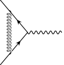
	(a)	(b)
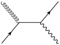
(c)	(d)	(e)	(f)

Figure 1: Parton-level subprocesses contributing to the Drell-Yan process at $\mathcal{O}(\alpha_{s})$: (a,b) virtual correction, (c,d) real gluon emission (e,f) quark-gluon Compton.

The expression for the square of the amplitude given below has been summed over the spin and colors of unobserved particles.

$$\left|M^{R}\right|^{2}=\delta_{\lambda_{q},-\lambda_{\bar{q}}}\,N_{c}\,C_{F}\,\left(\frac{4\pi\alpha g_{s}}{Q^{2}}\right)^{2}\,\left|f^{\lambda_{q}\lambda}\right|^{2}\,L^{\mu\nu}\,W^{R}_{\mu\nu}\ ,$$

where

$$W^{R}_{\mu\nu} = \frac{2}{\hat{t}^{2}}\left[2(p_{\bar{q}}\cdot k){\rm Tr}(\omega_{\lambda_{q}}k\gamma_{\mu}p_{q}\gamma_{\nu})-\kappa^{2}{\rm Tr}(\omega_{\lambda_{q}}p_{\bar{q}}\gamma_{\mu}p_{q}\gamma_{\nu})\right]$$ (7)

$$+ \,\frac{2}{\hat{u}^{2}}\left[2(p_{q}\cdot k){\rm Tr}(\omega_{\lambda_{q}}p_{\bar{q}}\gamma_{\mu}k\gamma_{\nu})-\kappa^{2}{\rm Tr}(\omega_{\lambda_{q}}p_{\bar{q}}\gamma_{\mu}p_{q}\gamma_{\nu})\right]$$

$$+ \,\frac{4}{\hat{t}\hat{u}}\left[\left(2p_{q}\cdot p_{\bar{q}}-2p_{q}\cdot k-2p_{\bar{q}}\cdot k\right)W^{T}_{\mu\nu}+(p_{q\mu}+p_{\bar{q}\mu})k^{\alpha}W^{T}_{\alpha\nu}\right.$$

$$\left.\hskip 144.0pt+\,W^{T}_{\mu\alpha}k^{\alpha}(p_{q\nu}+p_{\bar{q}\nu})\right]\ ,$$

The tree level hadronic and leptonic tensors $W^{T}_{\mu\nu}\,,\,L_{\mu\nu}$ were defined in the previous section and new invariant variables are introduced,

$$\hat{t}=(p_{q}-q)^{2}\ ,\,\hat{u}=(p_{\bar{q}}-q)^{2}\ .$$

In Eq.(7), we have dropped terms which do not contribute when $\kappa^{2}\to 0$. It should be noted that the $\kappa^{2}$ terms in the first and second lines can not be neglected since the phase space integral produces $1/\kappa^{2}$ singularity [20].

The cross section is given by,

$$d\hat{\sigma}^{R}=\frac{1}{2N_{c}^{2}s}\left|M^{R}\right|^{2}d\Phi_{3}\ ,$$ (8)

where $d\Phi_{3}$ is the three particle phase space. To integrate out the irrelevant variables in Eq.(8), we take the CM frame of $q\bar{q}$:

$$p_{q}=\frac{\sqrt{s}}{2}\,(1,0,0,1)\ ,\ p_{\bar{q}}=\frac{\sqrt{s}}{2}\,(1,0,0,-1)\ .$$

Parametrizing the momenta of lepton $l$ and lepton pair $q$ by,

$$l^{\mu} = |{\bf l}|\,(1\,,\,\sin\theta\cos\varphi\,,\,\sin\theta\sin\varphi\,,\,\cos\theta)\ ,$$

$$q^{\mu} = (q^{0}\,,\,{\bf q}\,\sin\hat{\theta}\cos\hat{\varphi}\,,\,{\bf q}\,\sin\hat{\theta}\sin\hat{\varphi}\,,\,{\bf q}\,\cos\hat{\theta})\ ,$$

where

$$q^{0} = \frac{s+Q^{2}-\kappa^{2}}{2\sqrt{s}}\qquad,\qquad|{\bf q}|^{2}=q^{02}-Q^{2}\ ,$$

$$|{\bf l}| = \frac{Q^{2}}{2\,\left[q^{0}-|{\bf q}|\,(\sin\hat{\theta}\sin\theta\cos(\hat{\varphi}-\varphi)+\cos\hat{\theta}\cos\theta)\right]}\ ,$$

it is easy to write the phase space element $d\Phi_{3}$ as,

$$d\Phi_{3}=\frac{|{\bf q}|\,Q^{2}\,dQ^{2}\,d\cos\hat{\theta}\,d\hat{\varphi}\,d\cos\theta\,d\varphi}{32\,(2\pi)^{5}\,\sqrt{s}\,\left[q^{0}-|{\bf q}|\,(\sin\hat{\theta}\sin\theta\cos(\hat{\varphi}-\varphi)+\cos\hat{\theta}\cos\theta)\right]^{2}}\ .$$

After integrating over the angular variables [10] and dropping terms which vanish when $\kappa^{2}\to 0$, we write the inclusive cross section for the polarized lepton in the following form:

$$\frac{d\hat{\sigma}^{R}(\lambda_{q},\lambda_{\bar{q}};\lambda)}{dQ^{2}\,d\cos\theta}=\frac{d\hat{\sigma}^{RT}(\lambda_{q},\lambda_{\bar{q}};\lambda;z)}{dQ^{2}\,d\cos\theta}\,F^{R}(Q^{2}\,,\,z)+\frac{d\hat{\sigma}^{RF}(\lambda_{q},\lambda_{\bar{q}};\lambda)}{dQ^{2}\,d\cos\theta}\ ,$$ (9)

where the first term contains the infrared and mass singularities as well as terms associated with them and,

$$\frac{d\hat{\sigma}^{RT}(\lambda_{q},\lambda_{\bar{q}};\lambda;z)}{dQ^{2}\,d\cos\theta}=\delta_{\lambda_{q},-\lambda_{\bar{q}}}\,\frac{\pi}{2N_{c}}\left(\frac{\alpha}{Q^{2}}\right)^{2}\left|f^{\lambda_{q}\lambda}\right|^{2}\cdot\frac{1}{2}$$

$$\times \left[\frac{8z^{2}}{(1+\cos\theta+z(1-\cos\theta))^{4}}\left\{(1+\lambda_{q}\lambda)(1+\cos\theta)^{2}+(1-\lambda_{q}\lambda)(1-\cos\theta)^{2}z^{2}\right\}\right.$$

$$+ \,\left.\frac{8z^{2}}{(1-\cos\theta+z(1+\cos\theta))^{4}}\left\{(1+\lambda_{q}\lambda)(1+\cos\theta)^{2}z^{2}+(1-\lambda_{q}\lambda)(1-\cos\theta)^{2}\right\}\right]\ .$$

with

$$F^{R}(Q^{2}\,,\,z) = \frac{\alpha_{s}}{\pi}C_{F}\,\left[\left(\frac{1}{2}\ln^{2}\frac{Q^{2}}{\kappa^{2}}-\frac{\pi^{2}}{6}\right)\delta(1-z)+\frac{1+z^{2}}{(1-z)}_{+}\ln\frac{Q^{2}}{\kappa^{2}}\right.$$

$$\hskip 60.0pt\left.+\,2(1+z^{2})\left(\frac{\ln{(1-z)}}{1-z}\right)_{+}-2(1+z^{2})\frac{\ln z}{1-z}-(1-z)\right]\ .$$

The second term in Eq.(9) gives the $\mathcal{O}(\alpha_{s})$ finite contribution whose explicit form is listed in Appendix A. It should be noted that the first (second) term in Eq.(3) is just the tree level cross section for the $q\,\bar{q}$ annihilation with momenta $zp_{q}$ and $p_{\bar{q}}$ ($p_{q}$ and $zp_{\bar{q}}$) times $z$ which arises from the difference between the flux normalizations. These terms express the processes with collinear gluon emissions. The function $F^{R}$ can be understood to be a probability to emit a collinear gluon with momentum $(1-z)p_{q}$ or $(1-z)p_{\bar{q}}$ and does not depend on the helicities of quarks because of the helicity conservation of QCD interaction.

By adding the tree level Eq.(5) and virtual Eq.(6) contributions to Eq.(9), the double logarithmic infrared singularities cancel out and the cross section from the $q\,\bar{q}$ initial states becomes,

$$\frac{d\hat{\sigma}^{T+V+R}}{dQ^{2}d\cos\theta} = \frac{d\hat{\sigma}^{RT}}{dQ^{2}d\cos\theta}\ \left[\left(1-\frac{7}{4}\,\frac{\alpha_{s}}{\pi}\,C_{F}\right)\delta(1-z)+\frac{\alpha_{s}}{\pi}\left(P_{qq}(z)\ln\frac{Q^{2}}{\kappa^{2}}\right.\right.$$ (11)

$$+\,\left.\left.C_{F}\left\{2(1+z^{2})\left(\frac{\ln{(1-z)}}{1-z}\right)_{+}-2(1+z^{2})\frac{\ln z}{1-z}-(1-z)\right\}\right)\right]$$

$$+ \frac{d\hat{\sigma}^{RF}}{dQ^{2}d\cos\theta}\ ,$$

where

$$P_{qq}(z)=C_{F}\left(\frac{1+z^{2}}{(1-z)_{+}}+\frac{3}{2}\delta(1-z)\right)\ ,$$

which is the DGLAP one-loop splitting functions $P_{qq}$. To obtain above result, we have used the fact,

$$\frac{d\hat{\sigma}^{RT}(\lambda_{q},\lambda_{\bar{q}};\lambda;z)}{dQ^{2}\,d\cos\theta}\,\delta(1-z)=\frac{d\hat{\sigma}^{T}(\lambda_{q},\lambda_{\bar{q}};\lambda)}{dQ^{2}\,d\cos\theta}\ .$$

Finally, the contribution from the quark-gluon Compton process (Fig.1e and 1f),

$$q(p_{q},\lambda_{q})+g(k,h)\to l(l,\lambda)+\bar{l}(l^{\prime},\lambda^{\prime})+q(p_{q}^{\prime},\lambda_{q}^{\prime})\ ,$$

where $h$ is the helicity of gluon, can be calculated in the same way as before. To avoid singularities in the physical region, the gluon mass is taken to be $-\kappa^{2}$ [20] and the spin projection for incoming gluons reads,

$$\epsilon_{\alpha}(k,h)\,\epsilon_{\beta}^{*}(k,h)=\frac{1}{2}\,\left[-g_{\alpha\beta}+i\,\epsilon_{\alpha\beta\gamma\delta}\,\frac{k^{\gamma}p^{\delta}_{q}}{k\cdot p_{q}}\right]\ .$$

The amplitude is,

$$M^{C} = \delta_{\lambda_{q},\lambda_{q}^{\prime}}\,\delta_{\lambda,-\lambda^{\prime}}\,\left(-\,\frac{e^{2}g_{s}}{Q^{2}}\right)\,f^{\lambda_{q}\lambda}\ \bar{u}_{\lambda}(l)\gamma^{\mu}v_{\lambda^{\prime}}(l^{\prime})$$

$$\times\ \bar{u}_{\lambda_{q}^{\prime}}(p_{q}^{\prime})\left[\gamma_{\mu}\frac{1}{\not{\!p}_{q}+\not{\!k}}\gamma_{\alpha}+\gamma_{\alpha}\frac{1}{\not{\!p}_{q}-\not{\!q}}\gamma_{\mu}\right]\,T^{a}\,u_{\lambda_{q}}(p_{q})\,\epsilon^{\alpha}_{a}(k,h)\ ,$$

and its square becomes,

$$\left|M^{C}\right|^{2}=N_{c}\,C_{F}\,\left(\frac{4\pi\alpha g_{s}}{Q^{2}}\right)^{2}\,\left|f^{\lambda_{q}\lambda}\right|^{2}\,L^{\mu\nu}\,W^{C}_{\mu\nu}\ ,$$

where

$$W^{C}_{\mu\nu}=\frac{1}{s}(1+\lambda_{q}h)\left(1+\frac{\hat{u}}{\hat{t}}\right){\rm Tr}(\omega_{\lambda_{q}}\,p_{q}^{\prime}\,\gamma_{\mu}\,k\,\gamma_{\nu})$$

$$+ \left\{\frac{2\hat{u}}{s\hat{t}}+\frac{1}{s}(1+\lambda_{q}h)+\frac{1}{\hat{t}}(1-\lambda_{q}h)\right\}{\rm Tr}(\omega_{\lambda_{q}}\,p_{q}^{\prime}\,\gamma_{\mu}\,p_{q}\,\gamma_{\nu})$$

$$- \frac{1}{\hat{t}}(1-\lambda_{q}h)\left(1+\frac{\hat{u}}{s}\right){\rm Tr}(\omega_{\lambda_{q}}\,k\,\gamma_{\mu}\,p_{q}\,\gamma_{\nu})+\,\frac{4}{\hat{t}}(1+\lambda_{q}h)p_{q\mu}^{\prime}p_{q\nu}^{\prime}+\frac{4}{s}(1-\lambda_{q}h)p_{q\mu}p_{q\nu}$$

$$+ \frac{\kappa^{2}}{\hat{t}^{2}}\left(1-\lambda_{q}h\,\frac{2Q^{2}-s}{s}\right){\rm Tr}(\omega_{\lambda_{q}}\,(p_{q}^{\prime}-k)\,\gamma_{\mu}\,p_{q}\,\gamma_{\nu})\ ,$$

with

$$s=(p_{q}+k)^{2}\ ,\ \hat{t}=(p_{q}-q)^{2}\ ,\ \hat{u}=(k-q)^{2}\ .$$

From the cross section formula for this process,

$$d\hat{\sigma}^{C}=\frac{1}{2N_{c}(N_{c}^{2}-1)s}\left|M^{C}\right|^{2}d\Phi_{3}\ ,$$

we obtain the polarized lepton distribution and write it in the same form as Eq.(9),

$$\frac{d\hat{\sigma}^{C}(\lambda_{q},h;\lambda)}{dQ^{2}\,d\cos\theta}=\frac{d\hat{\sigma}^{CT}(\lambda_{q};\lambda;z)}{dQ^{2}\,d\cos\theta}\,F^{C}(Q^{2}\,,\,z\,,\,\lambda_{q}\,,\,h)+\frac{d\hat{\sigma}^{CF}(\lambda_{q},h;\lambda)}{dQ^{2}\,d\cos\theta}\ .$$ (12)

The first term, in this case, is given by,

$$\frac{d\hat{\sigma}^{CT}(\lambda_{q};\lambda;z)}{dQ^{2}\,d\cos\theta}=\frac{\pi}{2N_{c}}\left(\frac{\alpha}{Q^{2}}\right)^{2}\,\left|f^{\lambda_{q}\lambda}\right|^{2}$$

$$\times \frac{8z^{2}}{(1-\cos\theta+z(1+\cos\theta))^{4}}\left\{(1+\lambda_{q}\lambda)(1+\cos\theta)^{2}z^{2}+(1-\lambda_{q}\lambda)(1-\cos\theta)^{2}\right\}\ ,$$

and

$$F^{C}(Q^{2}\,,\,z\,,\,\lambda_{q}\,,\,h)=\left(\frac{\alpha_{s}}{2\pi}\right)\,\left[P^{C}_{qg}(z;\lambda_{q},h)\left(\ln\frac{Q^{2}}{\kappa^{2}}+\ln\frac{1-z}{z^{2}}\right)-\frac{1}{4}(1+\lambda_{q}h(1-2z))\right]\ .$$

The quantity $P^{C}_{qg}$ is related to the unpolarized and polarized DGLAP splitting functions $P_{qg}(z)$ and $\Delta P_{qg}(z)$ in the following way,

$$P^{C}_{qg}(z;\lambda_{q},h)=\frac{1}{2}\left(P_{qg}(z)-\lambda_{q}h\Delta P_{qg}(z)\right)=\frac{(1+\lambda_{q}h)(1-z)^{2}+(1-\lambda_{q}h)z^{2}}{4}\ .$$

Equation (3) again expresses the tree level cross section for the $q\,\bar{q}$ annihilation with momenta $p_{q}$ and $zk$ where the $\bar{q}$ is emitted collinearly from the initial gluon. In contrast to the $q\,\bar{q}$ annihilation case, the function $F^{C}$ does depend on the helicities of initial quark and gluon since the emitted antiquark should have the helicity $\lambda_{\bar{q}}=-\lambda_{q}$ to annihilate into the electroweak gauge bosons. The remaining finite contribution $d\hat{\sigma}^{CF}$ can be found in Appendix A.

The cross section for the $\bar{q}\,g$ subprocess can be obtained by changing $(\lambda_{q},h)$ to $(-\lambda_{q},-h)$ and $\mu\leftrightarrow\nu$ in $W^{C}_{\mu\nu}$ in the above formulas.

From these results, the unpolarized cross sections are easily obtained. As a check, we have reproduced the results of Ref.[20] by neglecting the $Z$ boson contribution.

4 FACTORIZATION AND SCHEME CHANGE

Before proceeding to numerical studies, we must factorize the mass singularities into the parton densities in the $\overline{\rm MS}$ scheme since the two-loop evolution of them which should be combined with the one-loop corrections for the hard part, is given in this scheme.

The renormalized parton densities at the factorization scale $\mu_{F}^{2}$ which are relevant to this work are written as,

$$q(x,\mu_{F}^{2}) = \int_{x}^{1}\frac{dy}{y}\left[q(y)\left\{\delta\left(1-\frac{x}{y}\right)+\frac{\alpha_{s}}{2\pi}\left(P_{qq}\left(\frac{x}{y}\right)\ln\frac{\mu_{F}^{2}}{\kappa^{2}}+C_{qq}\left(\frac{x}{y}\right)\right)\right\}\right.$$

$$\hskip 78.0pt\left.+\,g(y)\frac{\alpha_{s}}{2\pi}\left(P_{qg}\left(\frac{x}{y}\right)\ln\frac{\mu_{F}^{2}}{\kappa^{2}}+C_{qg}\left(\frac{x}{y}\right)\right)\right]\ ,$$

$$\Delta q(x,\mu_{F}^{2}) = \int_{x}^{1}\frac{dy}{y}\left[\Delta q(y)\left\{\delta\left(1-\frac{x}{y}\right)+\frac{\alpha_{s}}{2\pi}\left(P_{qq}\left(\frac{x}{y}\right)\ln\frac{\mu_{F}^{2}}{\kappa^{2}}+C_{qq}\left(\frac{x}{y}\right)\right)\right\}\right.$$

$$\hskip 48.0pt\left.+\,\Delta g(y)\frac{\alpha_{s}}{2\pi}\left(\Delta P_{qg}\left(\frac{x}{y}\right)\ln\frac{\mu_{F}^{2}}{\kappa^{2}}+\Delta C_{qg}\left(\frac{x}{y}\right)\right)\right]\ ,$$

where $C$ and $\Delta C$ are finite functions depending on the scheme of factorization. Since the mass singularity is of universal nature and not affected by the lepton distributions, we can find the relation between different regularization schemes by comparing the results calculated in respective schemes for the simpler process. We have calculated the invariant mass distribution of lepton pair in our scheme and the results are shown in Appendix B. The same quantity has been calculated in the dimensional regularization scheme in Refs. [5, 7]. Note that the result depends on also the prescriptions of $\gamma_{5}$ in this scheme. We change our massive gluon scheme to the one adopted in Ref. [7] which can be combined with the known two-loop evolution equations for the parton densities in Refs. [22, 23]. We find,

$$C_{qq}^{\kappa^{2}\to\overline{\rm MS}}(z) = -\,C_{F}\left((1+z^{2})\frac{\ln z}{1-z}+2(1-z)+\left(\frac{\pi^{2}}{3}-\frac{9}{4}\right)\delta(1-z)\right)\ ,$$

$$C_{qg}^{\kappa^{2}\to\overline{\rm MS}}(z) = -\,\left(\frac{(1-z)^{2}+z^{2}}{2}\ln\left(z(1-z)\right)+1\right)\ ,$$

and

$$\Delta C_{qg}^{\kappa^{2}\to\overline{\rm MS}}(z)=-\left(\frac{2z-1}{2}\ln\left(z(1-z)\right)+\frac{1}{2}\right)\ .$$

We must,therefore, factorize these finite terms together with the singular terms from the subprocess cross sections.

The final results for the hard part at $\mathcal{O}(\alpha_{s})$ level in the $\overline{\rm MS}$ factorization scheme read for $q\bar{q}$ annihilation from Eq.(11),

$$\frac{d\hat{\sigma}^{q\bar{q}}(\mu_{F}^{2})}{dQ^{2}d\cos\theta} = \frac{d\hat{\sigma}^{RT}}{dQ^{2}d\cos\theta}\ \,\left[\left\{1+\frac{\alpha_{s}}{\pi}\,C_{F}\left(\frac{\pi^{2}}{3}-4\right)\right\}\delta(1-z)+\frac{\alpha_{s}}{\pi}\,\left(P_{qq}(z)\ln\frac{Q^{2}}{\mu_{F}^{2}}\right.\right.$$ (14)

$$+\,\left.\left.C_{F}\left\{2(1+z^{2})\left(\frac{\ln{(1-z)}}{1-z}\right)_{+}-(1+z^{2})\frac{\ln z}{1-z}+(1-z)\right\}\right)\right]$$

$$+ \,\frac{d\hat{\sigma}^{RF}}{dQ^{2}d\cos\theta}\ ,$$

and for $qg$ Compton process from Eq.(12),

$$\frac{d\hat{\sigma}^{qg}(\mu_{F}^{2})}{dQ^{2}\,d\cos\theta} = \frac{d\hat{\sigma}^{CT}}{dQ^{2}\,d\cos\theta}\,\frac{\alpha_{s}}{2\pi}\left[P^{C}_{qg}(z;\lambda_{q},h)\,\left\{\ln\frac{Q^{2}}{\mu_{F}^{2}}+\ln\frac{(1-z)^{2}}{z}\right\}\right.$$ (15)

$$\hskip 168.0pt+\,\left.\frac{1}{4}(1-2\lambda_{q}h(1-z))\right]$$

$$+ \,\frac{d\hat{\sigma}^{CF}}{dQ^{2}\,d\cos\theta}\ .$$

5 NUMERICAL RESULTS

We are now ready to predict the helicity distributions of lepton in proton-proton annihilation. By denoting the scattering angle of lepton in the CM frame of protons with momenta $P_{A}$ and $P_{B}$ by $\theta^{*}$, the relation between $\cos\theta$ in the CM frame of partons with momenta $x_{1}P_{A}$ and $x_{2}P_{B}$ and $\cos\theta^{*}$ reads,

$$\cos\theta=\frac{x_{2}(1+\cos\theta^{*})-x_{1}(1-\cos\theta^{*})}{x_{2}(1+\cos\theta^{*})+x_{1}(1-\cos\theta^{*})}\ .$$

The hadronic cross section for the helicity distribution of lepton is finally given by inserting Eqs.(14,15) in terms of $\theta^{*}$, into Eq.(1) and changing the parton densities into the $\mu_{F}^{2}$ dependent ones. We use the rapidity $y_{l}$ in stead of the scattering angle $\cos\theta^{*}$ of lepton in this section, which is defined by,

$$y_{l}=\frac{1}{2}\,\ln\,\frac{1+\cos\theta^{*}}{1-\cos\theta^{*}}\ .$$

We fix the total energy $S$ of the proton-proton system to be $\sqrt{S}=500$ GeV which is the planed highest energy at RHIC. Although our formulas can be applied to the process for arbitrary $Q$, we have chosen two values $Q=M_{Z}$ (the $Z$ boson pole) and $Q=10{\rm GeV}$ as typical examples. For the strong coupling constant, we use the standard two-loop form with $\Lambda_{\rm QCD}$ which is set to the value used in the parton densities. The following values for other parameters of the standard model are used:

$$\alpha = \frac{1}{128},\quad\sin^{2}\theta_{W}=0.2315\ ,$$

$$M_{Z} = 91.187\ {\rm GeV}\ ,\quad\Gamma_{Z}=2.5\ {\rm GeV}\ .$$

Denoting the helicities of initial protons by $P_{A,B}(\pm)$, there are three cases to be analyzed corresponding to $P_{A}(+)P_{B}(-)$, $P_{A}(+)P_{B}(+)$, $P_{A}(-)P_{B}(-)$ configurations.

We have organized this section as follows. Firstly, we show the numerical results for the helicity distributions of lepton with respect to $y_{l}$. Secondly, we investigate the factorization scale and the parton parametrization dependence of the cross section.

5.1 The Lepton Helicity Distribution

Here we use the $\overline{\rm MS}$ parameterization of the parton densities in Refs.[24, 25] and take the factorization scale $\mu_{F}$ and the renormalization scale $\mu_{R}$ to be $\mu_{F}=\mu_{R}=Q$. The scale dependence will be discussed later.

We give in Fig.2 the results at $Q=M_{Z}$

Figure 2: The cross sections for leptons with negative and positive helicity in the three configurations for the spins of protons with respect to $y_{l}$ for $Q=M_{Z}$.

for both distributions of leptons with negative and positive helicities in the three $P_{A}(+)P_{B}(-)$, $P_{A}(+)P_{B}(+)$, $P_{A}(-)P_{B}(-)$ configurations. The unit of the cross section (vertical axis) is [pb/GeV]. The dotted line is the total contribution. The solid line is the contribution from the $u$-quark, namely $u\bar{u}$ and $ug(\bar{u}g)$ annihilation sub-processes, whereas the dot-dashed line from the $d$-quark sector: we write simply $d$ for the $d$ and $s$ quarks. The long dashed (dashed) line is the contribution from the tree level $u\bar{u}$ ($d\bar{d}$). We plot in Fig.3 the similar results for $Q=10$ GeV. Some comments are in order for these results. Firstly, the main effect of QCD correction is just an enhancement of the tree level cross section: the $K$ factor is $1.5\sim 1.8$. It does not change significantly the shape of the lepton distributions from the tree level one.

Figure 3: The cross sections for leptons with negative and positive helicity in the three configurations for the spins of protons with respect to $y_{l}$ for $Q=10$ GeV.

Secondly, we see that the $u$ and $d$ quarks give different and characteristic contributions to the helicity distributions for lepton. In particular, the case of the lepton distribution in the $P_{A}(+)P_{B}(-)$ configuration for $Q=M_{Z}$ deserves some explanations. Our numerical results show that in the negative rapidity region, the leptons with negative helicities are mainly produced and those come from the $u$-quark annihilation. On the other hand, in the positive rapidity region, leptons with both helicities are produced, however the leptons with negative helicities come mainly from the $d$-quark annihilation subprocesses. These features can be understood intuitively by observing the following aspects. (1) The polarized quark distributions in the polarized proton $P(+)$ roughly satisfy for the relevant scale $Q^{2}=M_{Z}^{2}$ and the momentum fractions of partons $x_{1}x_{2}=M_{Z}^{2}/S$,

$$u(\uparrow)\gg d(\downarrow)\sim u(\downarrow)\gg d(\uparrow)\gg\bar{u}(\uparrow,\downarrow)\sim\bar{d}(\uparrow,\downarrow)\ ,$$

where $\uparrow$ and $\downarrow$ denote the quark’s spin parallel and anti-parallel to the parent proton’s spin. This relation implies the dominant subprocesses in the $P_{A}(+)P_{B}(-)$ configuration to be (i) $u_{A}(\uparrow)\bar{u}_{B}$, (ii) $\bar{u}_{A}u_{B}(\uparrow)$, (iii) $d_{A}(\downarrow)\bar{d}_{B}$ and (iv) $\bar{d}_{A}d_{B}(\downarrow)$. (2) From the angular momentum conservation, the spin of produced $Z$ boson is aligned to $P_{A}$ ($P_{B}$) direction for $u_{A}\bar{u}_{B}$ and $\bar{u}_{A}u_{B}$ ($d_{A}\bar{d}_{B}$ and $\bar{d}_{A}d_{B}$) annihilations and the negative (positive) helicity lepton from the $Z$ decay has higher probability to be produced in the opposite (same) direction of $Z$ boson’s spin. (3) The third point to be noted is that the $V-A$ coupling is larger than the $V+A$ coupling for the quark-$Z$ boson interaction. This suggests that among four subprocesses in (1), (ii) and (iii) eventually dominate the process. (4) Finally, since the momentum fractions of quarks are bigger than those of anti-quarks, the distributions of negative helicity lepton from (ii) and (iii) are Lorentz boosted to the negative and positive rapidity regions respectively. The fact above (3) also explains that the $d$ ($u$) quark contribution is larger than that of $u$ ($d$) quark for the $P_{A}(+)P_{B}(+)$ ($P_{A}(-)P_{B}(-)$) configuration. For these configurations, the lepton distribution is symmetric around $y_{l}=0$ as it should be.

At the lower value of $Q$ ($Q=10$ GeV), the $Z$ boson contribution can be safely neglected and the electromagnetic interaction becomes dominant. In this case, the situation is not so simple as the previous one ($Q=M_{Z}$). At first sight, only the point (3) above should be dropped. If so, the subprocess (i) and (ii) had dominated the process which leaded to the similar distributions as those for the $Q=M_{Z}$ case. However, the distribution takes somehow different shape due to the following reasons. For $Q=10$ GeV, the partons with very small momentum fractions participate in the process ($x_{1}x_{2}=10^{2}/S$). Therefore, for the “dominant“  processes for the $Q=M_{Z}$ case, (i) and (ii), the Lorentz boost effect is fairly large and the Jacobian factor $J=\sin^{2}\theta^{*}$ apparently diminishes the cross section in the $y_{l}$ distributions. Furthermore at this scale, all subprocesses seem to contribute equally to the cross section and the partons with small $x$ have less information on the spin of the parent proton. One can see, nonetheless, the contribution from the antisymmetric part of the hadronic tensor which causes the asymmetric distributions of lepton for the $P_{A}(+)P_{B}(-)$ configuration.

We also estimate the lepton helicity asymmetry $A_{l}$ which is defined by,

$$A_{l}\equiv\frac{d\sigma(\lambda=-1)-d\sigma(\lambda=+1)}{d\sigma(\lambda=-1)+d\sigma(\lambda=+1)}\ .$$

This asymmetry is plotted in Fig. 4 for the three spin configurations for protons. The upper three graphs show the asymmetry for the $Q=M_{Z}$ case and the lower three for the $Q=10$ GeV case.

Figure 4: The helicity asymmetry in the three configurations for the spins of protons with respect to $y_{l}$.

The solid line is the $\mathcal{O}(\alpha_{s})$ result and the long-dashed line is the tree level one. In these results, we recognize that there are non negligible effects from the QCD higher order corrections other than just the enhancement effects of tree level results. This asymmetry amounts to around 20 - 30% in the central rapidity region for $Q=M_{Z}$. The asymmetry for $Q=10$ GeV is much smaller than that for $Q=M_{Z}$. This is consistent with the previous observation that partons with small $x$ which do not have enough spin information of parent proton, contribute to the process at smaller $Q$.

5.2 The Scale and Parametrization Dependence

The physical quantities such as the cross sections or asymmetries are obviously independent of the renormalization and the factorization scales. However the truncation of the perturbative series at a fixed order induces the dependence on these scales which leads to uncertainty in the theoretical predictions. We study the scale dependence of the cross section and asymmetry by comparing the results obtained with three different choices for the scale: $\mu_{F}^{2}=2\,Q^{2}$, $\mu_{F}^{2}=Q^{2}$ and $\mu_{F}^{2}=0.5\,Q^{2}$. We will also mention the dependence on the various parton parametrizations in this subsection.

We give the results only for the case of $P_{A}(+)P_{B}(-)$ configuration with $Q=M_{Z}$ since the results for other spin configurations of protons and the value of $Q$, are found to be essentially the same.

Figure 5: The scale and the parton parametrization dependence.

The scale dependence of the lepton distributions (the upper two graphs) as well as the asymmetry (the lower left graph) is shown in Fig. 5 where the dashed line corresponds to $\mu_{F}^{2}=2\,Q^{2}$, the solid line to $\mu_{F}^{2}=Q^{2}$ and the dotted line to $\mu_{F}^{2}=0.5\,Q^{2}$. In this calculation, we use the parton densities in Ref. [24]. One can see that the variation is less than 10% in the central rapidity region.

For the parton parametrization dependence, we calculate the asymmetry with the three sets in Ref. [26] since the difference appears more clearly in the asymmetry than in the cross sections. The results are shown in Fig. 5 (the lower right graph). The solid line, dashed line and dotted line correspond to GS-A, GS-B and GS-C respectively. The dependence on the parton parametrizations is similar to the scale dependence in size and not so large. The reason will be that the process is dominated by the quark and anti-quark annihilation in the RHIC energy region and the gluon initiated Compton subprocess, in which the ambiguity of gluon distribution will appear, gives a tiny correction to the cross section.

6 CONCLUSION

We have presented a complete calculation at the ${\cal O}(\alpha_{s})$ order in QCD of the lepton helicity distributions in the polarized Drell-Yan process. We have numerically analyzed the cross section at $Q=10$ GeV and $Q=M_{Z}$ and pointed out that the $u(\bar{u})$ and $d(\bar{d})$ quarks give different and characteristic contributions to the lepton helicity distributions which deserve some theoretical interests. The QCD corrections mainly enhance the tree level cross sections and this fact can explain qualitatively the lepton helicity distributions from the various proton’s spin configurations. We have defined and estimated the lepton helicity asymmetry which amounts to around 20-30%.

We have also studied the dependence of the cross section and the asymmetry on the scale and parton parametrization. Since the $q\,\bar{q}$ subprocess is dominant in the RHIC energy region, we will not be able, unfortunately, to find clear difference between various parton parameterizations which have big ambiguities in the gluon distributions.

From the experimental point of view, it seems rather difficult to measure the helicity of produced muon and/or electron in the Drell-Yan process. However, if we can observe the $\tau$ lepton produced from the Drell-Yan process and its decay, we will be able to compare the experimental data and theoretical prediction presented in this paper. We believe that our calculations and numerical studies may provide a complementary information to the existing results for the invariant mass and rapidity or $x_{F}$ distributions of lepton pair in the polarized proton-proton collisions.

ACKNOWLEDGMENTS

We are grateful to Werner Vogelsang for useful discussions and suggestions. We would like to thank T. D. Lee and W. Vogelsang for hospitality and support extended to them at RIKEN-BNL Research Center where part of this work was performed. J. K. thank J. Blümlein for hospitality and support extended to him at DESY where this work has been completed. The work of J. K. was supported in part by the Monbu-kagaku-sho Grant-in-Aid for Scientific Research No. C-13640289.

APPENDIX A: THE CROSS SECTION FORMULAE

The explicit forms for the finite contributions to the cross sections are listed in this appendix. We use the abbreviation $c\equiv\cos\theta$.

1. The real gluon emission process.

$$\frac{d\hat{\sigma}^{RF}(\lambda_{q},\lambda_{\bar{q}};\lambda)}{dQ^{2}d\cos\theta}=\delta_{\lambda_{q},-\lambda_{\bar{q}}}\,\frac{\pi}{2N_{c}}\left(\frac{\alpha}{Q^{2}}\right)^{2}\left|f^{\lambda_{q}\lambda}\right|^{2}\,\left(\frac{\alpha_{s}}{\pi}C_{F}\right)$$

$$\times \biggl{[}4z^{2}\frac{1+z^{2}}{1-z}\biggl{\{}\frac{(1+\lambda_{q}\lambda)(1+c)^{2}z^{2}+(1-\lambda_{q}\lambda)(1-c)^{2}}{(1-c+z(1+c))^{4}}\ln{\left(\frac{(1-c+z(1+c))^{2}}{4z}\right)}$$

$$\hskip 48.0pt+\,\frac{(1+\lambda_{q}\lambda)(1+c)^{2}+(1-\lambda_{q}\lambda)z^{2}(1-c)^{2}}{(1+c+z(1-c))^{4}}\ln{\left(\frac{(1+c+z(1-c))^{2}}{4z}\right)}\biggr{\}}$$

$$-\,2z(1-z)+\frac{4z(1-z)(1+z^{2})\left\{(1+z)^{2}-c^{2}(1+6z+z^{2})\right\}}{(1+c+z(1-c))^{2}(1-c+z(1+c))^{2}}$$

$$+\,\frac{8\lambda_{q}\lambda z^{2}(1-z)c}{(1+c+z(1-c))^{3}(1-c+z(1+c))^{3}}\left\{(1+z)^{2}(7-4z+7z^{2})\right.$$

$$\hskip 48.0pt\left.-\,2c^{2}(3+14z+10z^{2}+14z^{3}+3z^{4})-c^{4}(1-z)^{2}(1+z^{2})\right\}$$

$$+\,\frac{2z(1-z)}{3(1+c+z(1-c))^{4}(1-c+z(1+c))^{4}}$$

$$\hskip 24.0pt\times\,\left\{-(1+z)^{4}(1+14z-18z^{2}+14z^{3}+z^{4})\right.$$

$$\hskip 48.0pt+\,2c^{2}(1+z)^{2}(1+4z+239z^{2}-56z^{3}+239z^{4}+4z^{5}+z^{6})$$

$$\hskip 48.0pt+\,8c^{4}z(3-45z-151z^{2}-118z^{3}-151z^{4}-45z^{5}+3z^{6})$$

$$\hskip 48.0pt-\,2c^{6}(1-z)^{2}(1+8z+71z^{2}+48z^{3}+71z^{4}+8z^{5}+z^{6})$$

$$\hskip 168.0pt\left.+\,c^{8}(1-z)^{4}(1-2z+6z^{2}-2z^{3}+z^{4})\right\}\biggr{]}\ .$$

2. The quark gluon Compton process.

$$\frac{d\hat{\sigma}^{CF}(\lambda_{q},h;\lambda)}{dQ^{2}d\cos\theta}=\frac{\pi}{2N_{c}}\left(\frac{\alpha}{Q^{2}}\right)^{2}\left|f^{\lambda_{q}\lambda}\right|^{2}\,\left(\frac{\alpha_{s}}{\pi}\right)$$

$$\times \left[4\,z^{2}\,P^{C}_{qg}(z;\lambda_{q},h)\,\frac{(1+\lambda_{q}\lambda)(1+c)^{2}z^{2}+(1-\lambda_{q}\lambda)(1-c)^{2}}{(1-c+z(1+c))^{4}}\right.$$

$$\hskip 216.0pt\times\,\ln\left(\frac{(1-c+z(1+c))^{2}}{4z}\right)$$

$$\left.+\,\frac{2z(1-z)(1-z^{2}-c(1+6z+z^{2}))}{(1+c+z(1-c))(1-c+z(1+c))^{3}}\right.$$

$$\hskip 24.0pt\left.\times\,\biggl{\{}\left((1-\lambda_{q}\lambda)(1-c)+(1+\lambda_{q}\lambda)z(1+c)\right)P^{C}_{qg}(z;\lambda_{q},h)\right.$$

$$\hskip 72.0pt\left.-\,\frac{z}{2}\left((1-\lambda_{q}h)z(1-c)+(1+\lambda_{q}h)(1+c+z(1-c))\right)\biggr{\}}\right.$$

$$\left.+\,\frac{1}{4}(1+\lambda_{q}\lambda)(1-\lambda_{q}h)z^{2}\left(1-z-c\ln z\right)\right.$$

$$\left.+\,\frac{2\,z\,(1-z^{2})\,c\,P^{C}_{qg}(z;\lambda_{q},h)}{(1+c+z(1-c))(1-c+z(1+c))}+G_{S}+\lambda_{q}\lambda G_{A}\right]\ ,$$

where,

$$G_{S} = \frac{z(1-z)}{12(1+c+z(1-c))(1-c+z(1+c))^{4}}$$

$$\times \left[(1-z^{2})\left((1-\lambda_{q}h)(1+5z+21z^{2}-7z^{3}-2z^{4})\right.\right.$$

$$\left.\hskip 144.0pt-\,2(1+\lambda_{q}h)(1+2z-42z^{2}+2z^{3}+z^{4})\right)$$

$$-\,c\left((1-\lambda_{q}h)(4+16z+61z^{2}+98z^{3}-34z^{4}+2z^{5}-3z^{6})\right.$$

$$\left.\hskip 144.0pt-\,4(1+\lambda_{q}h)(1-3z^{2}-92z^{3}-3z^{4}+z^{6})\right)$$

$$+\,c^{2}\left((1-\lambda_{q}h)(5+17z+65z^{2}+208z^{3}+13z^{4}-17z^{5}-3z^{6})\right.$$

$$\left.\hskip 144.0pt-\,72(1+\lambda_{q}h)z^{2}(1-z^{2})\right)$$

$$-\,2c^{3}\left((1-\lambda_{q}h)z(4+13z+38z^{2}+16z^{3}-2z^{4}+3z^{5})\right.$$

$$\left.\hskip 144.0pt+\,2(1+\lambda_{q}h)(1-z)^{2}(1-2z-2z^{3}+z^{4})\right)$$

$$-\,c^{4}(1-z^{2})\left((1-\lambda_{q}h)(5-7z+7z^{2}+13z^{3})\right.$$

$$\left.\hskip 144.0pt-\,2(1+\lambda_{q}h)(1-z)^{2}(1-4z+z^{2})\right)$$

$$+\,c^{5}(1-\lambda_{q}h)(1-z)^{2}(4+3z^{2}+4z^{3}+3z^{4})$$

$$\left.-\,c^{6}(1-\lambda_{q}h)(1+z)(1-z)^{3}(1-z+z^{2})\right]$$

$$G_{A} = \frac{z(1-z)}{4(1+c+z(1-c))(1-c+z(1+c))^{3}}$$

$$\times \left[(1-z^{2})(1+4z+z^{2})\left(-(1-\lambda_{q}h)z+2(1+\lambda_{q}h)(1-z)\right)\right.$$

$$+\,2c\left((1-\lambda_{q}h)z(1+2z+4z^{2}+z^{4})-2(1+\lambda_{q}h)(1+3z^{2}-3z^{3}-z^{5})\right)$$

$$+\,2c^{2}(1-z)\left((1-\lambda_{q}h)z^{2}(1-2z-z^{2})+(1+\lambda_{q}h)(1-z^{4})\right)$$

$$-\,2c^{3}z(1-z)\left((1-\lambda_{q}h)(1+z+3z^{2}+z^{3})+2(1+\lambda_{q}h)(1-z)^{2}\right)$$

$$\left.+\,c^{4}(1-\lambda_{q}h)z(1-z)^{2}(1+z^{2})\right]\ .$$

APPENDIX B: THE INVARIANT MASS DISTRIBUTIONS

Here we present the invariant mass distribution of lepton pair in the massive gluon scheme before factorizing the mass singularity. Comparing these expressions with those in the dimensional regularization, we can find the relation between two regularization schemes.

1. The quark and antiquark annihilation process.

$$\frac{d\hat{\sigma}^{T+V+R}}{dQ^{2}} = \delta_{\lambda_{q},-\lambda_{\bar{q}}}\,\frac{4\pi}{3N_{c}}\left(\frac{\alpha}{Q^{2}}\right)^{2}\left|f^{\lambda_{q}\lambda}\right|^{2}$$

$$\times z\,\left[\left(1-\frac{7}{4}\,\frac{\alpha_{s}}{\pi}\,C_{F}\right)\delta(1-z)+\frac{\alpha_{s}}{\pi}\left(P_{qq}(z)\ln\frac{Q^{2}}{\kappa^{2}}\right.\right.$$

$$\quad+\,\left.\left.C_{F}\left\{2(1+z^{2})\left(\frac{\ln{(1-z)}}{1-z}\right)_{+}-2(1+z^{2})\frac{\ln z}{1-z}-2(1-z)\right\}\right)\right]\ .$$

2. The quark gluon Compton process.

$$\frac{d\hat{\sigma}^{C}}{dQ^{2}} = \frac{4\pi}{3N_{c}}\left(\frac{\alpha}{Q^{2}}\right)^{2}\left|f^{\lambda_{q}\lambda}\right|^{2}\,z\,\left(\frac{\alpha_{s}}{2\pi}\right)\,\left[P^{C}_{qg}(z;\lambda_{q},h)\left(\ln\frac{Q^{2}}{\kappa^{2}}+\ln\frac{1-z}{z^{2}}\right)\right.$$

$$\hskip 144.0pt\left.-\,\frac{1}{8}\left(1-2z+3z^{2}+\lambda_{q}h\left\{3-2z-3z^{2}\right\}\right)\right]\ .$$

References

• [1] European Muon Collab., J. Ashman et.al., Phys. Lett. B206 (1988) 364.
• [2] G.Bunce, N.Saito, J.Soffer and W.Vogelsang, Ann. Rev. Nucl. Part. Sci. 50 (2000) 525.
• [3] S. D. Drell and T. M. Yan, Phys. Rev. Lett.25 (1970) 316; Ann. Phys.66 (1971) 578.
• [4] P. Ratcliffe, Nucl. Phys. B233 (1982) 45.
• [5] A. Weber, Nucl. Phys. B382 (1992) 63.
• [6] B. Kamal, Phys. Rev. D53 (1996) 1142.
• [7] T. Gehrmann, Nucl. Phys.B498 (1997) 245.
• [8] J. P. Ralston and D.E. Soper Nucl. Phys. B152 (1979) 109.
• [9] R. L. Jaffe and X. Ji, Nucl. Phys. B375 (1992) 527.
• [10] W. Vogelsang and A. Weber, Phys. Rev. D48 (1993) 2073.
• [11] A. P. Contogouris, B. Kamal and Z. Merebashvili, Phys. Lett. B337 (1994) 169.
• [12] D. Sivers, Phys. Rev. D51 (1995) 4880.
• [13] C. Bourrely and J. Soffer, Phys. Lett. B314 (1993) 132; Nucl. Phys. B423 (1994) 329.
• [14] B. Kamal, Phys. Rev. D57 (1998) 6663.
• [15] T. Gehrmann, Nucl. Phys. B534 (1998) 21.
• [16] J. Soffer and P. Taxil, Phys. Lett. B85 (1979) 404; Nucl. Phys. B172 (1980) 106.
• [17] N. S. Craigie, K. Hidaka, M. Jacob and F. M. Renard, Phys. Rep. 99 (1983) 69.
• [18] E. Di Salvo, Eur. Phys. J. C19 (2001) 503.
• [19] H. Kitagawa, Y. Sakemi and T. Yamanishi, arXiv:hep-ph/0212377.
• [20] J. Kubar, M. Le Bellac, J.L.Meunier and G.Plaut, Nucl. Phys. B175 (1980) 251.
• [21] See e.g. R.D.Field, Applications of Perturbative QCD (Frontiers in Physics, Vol.77), Harpercollins (Sd) (1989/06/01)
• [22] W. Vogelsang, Phys. Rev. D54 (1996) 2023; Nucl. Phys. B475 (1996) 47.
• [23] R. Mertig and W. L. van Neerven, Z. Phys. C70 (1996) 637.
• [24] M. GlΓΌck, E. Reya, M. Stratmann and W. Vogelsang, Phys. Rev. D63 (2001) 094005.
• [25] A. D. Martin, R. G. Roberts, W. J. Stirling and R. S. Thorne, Eur. Phys. J. C14 (2000) 133.
• [26] T. Gehrmann and W. J. Stirling, Phys. Rev. D53 (1996) 6100.