RUB-TP2-19/03

1 Introduction

Deeply Virtual Compton Scattering (DVCS) attracts a large amount of interest, both experimentally and theoretically. The initial results on DVCS have been reported by HERMES [1], ZEUS [2] and H1 [3] experiments at DESY and the CLAS experiment [4] at TJNAF; the recent progress in the theoretical understanding of DVCS is summarized in the review articles [5],[6],[7].

DVCS on a given target accesses new non-perturbative objects – Generalized Parton Distributions (GPDs) of the target. These distributions contain encoded information on the quark-gluon structure of the target.

To date most of the experimental and theoretical work dedicated to DVCS concern with nucleon and pion targets. However, there are already first data on DVCS on nuclear (Deuterium, Neon) targets taken at HERMES [8]. On the theoretical side, nuclear GPDs may allow one to better understand the nature of nuclear forces [9].

Previously, the impulse approximation approach to nuclear effects in coherent DVCS on Deuterium and other spin-1 nuclei was considered in Refs. [10]. The aim of this paper is to apply the impulse approximation to DVCS on spin-0 nuclei and, in particular, to obtain a qualitative estimate of the Fermi motion effect on the beam-charge asymmetry for DVCS a spinless nucleus of Neon that was recently measured at HERMES [8].

In order to make clear the principal steps of the derivation, we first consider the calculation of the electromagnetic form factor of a spinless nucleus.

2 Electromagnetic form factor of a spinless nucleus

The electromagnetic (charge) form factor of a spinless nucleus, $F^{e.m.}_{A}(t)$, is defined using the matrix element of the operator of the electromagnetic current, $J^{\mu}(0)$, between the states of the initial and final nucleus with momenta $P_{A}$ and $P_{A}^{\prime}=P_{A}+q$ ($t\equiv q^{2}<0$):

$$\langle P_{A}+q|J^{\mu}(0)|P_{A}\rangle=(2P_{A}+q)^{\mu}F^{e.m.}_{A}(t)\,.$$ (1)

The matrix element in Eq. (1) can be evaluated using the impulse approximation which is based on the intuitive picture that the interaction with the nucleus is a two-step process: First, the nucleus is decomposed into non-relativistically moving nucleons; then, these nucleons interact independently with the probe. As a result, the matrix elements between the nuclear states can be expressed in terms of the nucleon matrix elements.

The consistent derivation of the impulse approximation and discussion of its limitations was given in Ref. [11]. In what follows, we shall present a less rigorous treatment of the impulse approximation. It is convenient to start from the covariant expression for the matrix element in Eq. (1) (see Ref. [12])

$$\langle P_{A}+q|J^{\mu}(0)|P_{A}\rangle=\sum_{{\rm nucleons}}\int\frac{d^{4}p_{1}}{i(2\pi)^{4}}\dots\frac{d^{4}p_{A}}{i(2\pi)^{4}}\bar{\Gamma}_{A}(p_{1}+q,p_{2},\dots,p_{A})$$

$$\times\Big{(}\frac{-1}{\hat{p_{1}}+\hat{q}-m}\Big{)}\hat{\Gamma}_{e.m.}^{\mu}(q)\Big{(}\frac{-1}{\hat{p_{1}}-m}\Big{)}\frac{(-1)^{A-1}}{(\hat{p_{2}}-m)\dots(\hat{p_{A}}-m)}\Gamma_{A}(p_{1},p_{2},\dots,p_{A})$$

$$\times i(2\pi)^{4}\delta^{4}(P_{A}-p_{1}-\dots-p_{A})\,,$$ (2)

with $\sum_{{\rm nucleons}}$ the incoherent sum of electromagnetic interactions with each nucleon, $\bar{\Gamma}_{A}$ and $\Gamma_{A}$ the covariant vertex functions describing the transition of $A$ nucleons to the nucleus, and $\hat{\Gamma}_{e.m.}^{\mu}$ the electromagnetic vertex of the nucleon,

$$\hat{\Gamma}_{e.m.}^{\mu}(q)=\gamma^{\mu}F_{1}(t)+\frac{i\sigma^{\mu\nu}q_{\nu}}{2m}F_{2}(t)\,,$$ (3)

where $F_{1}$ and $F_{2}$ are the nucleon elastic form factors; $m$ is the nucleon mass.

The covariant vertices $\bar{\Gamma}_{A}$ and $\Gamma_{A}$ in Eq. (2) can be related to non-relativistic nuclear wave function of the target. This non-relativistic reduction of Eq. (2) can be carried out as follows.

Firstly, there are $A$ four-dimensional integrations in Eq. (2). One integral (over $p_{1}$) is taken using the energy-momentum delta-function. Other $A$ integrals over energies of the spectator nucleons are taken in the approximation that only non-relativistic nucleons with positive energy are present in the nuclear wave function. This enables one to take the residue over the nucleon mass pole, for instance,

$$\int\frac{dp_{2}^{0}}{(p_{2})^{2}-m^{2}+i\epsilon}=-i\frac{2\pi}{2m}\,.$$ (4)

This procedure puts all spectator nucleons on their mass shell. Moreover, because of the energy-momentum conservation at each nuclear vertex, the interacting nucleon is also on the mass shell (ignoring small nuclear binding).

Secondly, since all nucleons are on the mass shell, the Dirac spinors in the propagators of the bound nucleons can be replaced with those of the free ones:

$$\hat{p}+m=\sum_{i}u^{(i)}(p)\bar{u}^{(i)}(p)\,.$$ (5)

Thirdly, the covariant nuclear vertex functions $\bar{\Gamma}_{A}$ and $\Gamma_{A}$ are expressed in terms of the corresponding non-relativistic nuclear wave function, $\Phi_{A}$, for instance

$$\bar{u}^{(\beta)}(p_{1})\bar{u}^{(i_{2})}(p_{2})\dots\bar{u}^{(i_{A})}(p_{A})\Gamma_{A}=\Big{(}(2\pi)^{3}2m\Big{)}^{\frac{A-1}{2}}(p_{1}^{2}-m^{2})\Phi_{A}(p_{1},\beta;p_{2},i_{2};\dots;p_{A},i_{A})\,.$$ (6)

Note that the nuclear wave function is normalized to the number of nucleons $A$. With Eqs. (4)-(6) in mind, the expression for the matrix element in Eq. (2) simplifies

$$\langle P_{A}+q|J^{\mu}(0)|P_{A}\rangle=\sum_{{\rm nucleons}}\int d^{3}p_{i}\sum_{\alpha,\beta}\Phi_{A}^{\ast}(p_{1}+q,\alpha)\Phi_{A}(p_{1},\beta)\bar{u}^{(\alpha)}(p_{1}+q)\hat{\Gamma}_{e.m.}^{\mu}(q){u}^{(\beta)}(p_{1})\,.$$ (7)

Here $d^{3}p_{i}$ denotes $A-1$ 3-dimensional integrals, $d^{3}p_{i}=d^{3}p_{2}\dots d^{3}p_{A}$. Also we keep only the momentum and spin indices of the struck nucleon in the argument of the nuclear wave function; summation over the polarization of the spectator nucleons is assumed.

For a spinless nucleus, only the terms with $\alpha=\beta$ survive in the product $\Phi_{A}^{\ast}(p_{1}+q,\alpha)\Phi_{A}(p_{1},\beta)$. Introducing the nuclear wave function averaged over polarization of its nucleons, $\Phi_{A}(p_{1})$,

$$\Phi_{A}(p_{1},\beta)=\frac{1}{\sqrt{2}}\Phi_{A}(p_{1})\,,$$ (8)

we arrive at

$$\langle P_{A}+q|J^{\mu}(0)|P_{A}\rangle = \frac{1}{2}\sum_{{\rm nucleons}}\int d^{3}p_{i}\Phi_{A}^{\ast}(p_{1}+q)\Phi_{A}(p_{1})\sum_{\alpha}\bar{u}^{(\alpha)}(p_{1}+q)\hat{\Gamma}_{e.m.}^{\mu}(q){u}^{(\alpha)}(p_{1})$$ (9)

$$= \frac{1}{2}\sum_{{\rm nucleons}}\int d^{3}p_{i}\Phi_{A}^{\ast}(p_{1}+q)\Phi_{A}(p_{1}){\rm Tr}\Big{(}\hat{\Gamma}_{e.m.}^{\mu}(q)\hat{P}(p_{1},q)\Big{)}\,,$$

where $\hat{P}(p_{1},q)$ is some sort of ”off-forward propagator”, $\hat{P}(p_{1},q)=\sum_{\alpha}{u}^{(\alpha)}(p_{1})\bar{u}^{(\alpha)}(p_{1}+q)$. This propagator can be decomposed in the basis of Dirac matrices with the result

$$\hat{P}(p_{1},q)=\hat{p}_{1}+\hat{q}/2+m+\hat{p}_{1}\hat{q}/(2m)\,.$$ (10)

Using the definition of $\hat{\Gamma}_{e.m.}^{\mu}$ in terms of the form factors $F_{1}(t)$ and $F_{2}(t)$ and then taking the trace of Dirac matrices in Eq. (9), we obtain

$$\langle P_{A}+q|J^{\mu}(0)|P_{A}\rangle=(2P_{A}+q)^{\mu}F^{e.m.}_{A}(t)=\sum_{{\rm nucleons}}\int d^{3}p_{i}\Phi_{A}^{\ast}(p_{1}+q)\Phi_{A}(p_{1})(2p_{1}+q)^{\mu}G_{E}(t)\,,$$ (11)

where the nucleon charge form factor is introduced, $G_{E}(t)=F_{1}(t)+t/(4m^{2})F_{2}(t)$. As a result of the non-relativistic reduction, Eq. (11) is intrinsically reference frame dependent and it is good only with accuracy ${\cal O}(p_{1}^{2}/m^{2})$. For a more consistent treatment, one would need to use the light-cone (infinite-momentum frame) description of the nuclear wave function, see reviews in [11, 13].

In the non-relativistic for $t=0$ we can use with accuracy ${\cal O}(p_{1}^{2}/m_{N}^{2})$ the $\mu=0$ component of Eq. (11) to fix normalization of the wave function

$$F^{e.m.}_{A}(0)=\frac{m}{M_{A}}\sum_{{\rm nucleons}}\int d^{3}p_{i}|\Phi_{A}(p_{1})|^{2}G_{E}(0)=\frac{ZG_{E}^{p}(0)}{A}\int d^{3}p_{i}|\Phi_{A}^{\ast}(p_{1})|^{2}=Z\,.$$ (12)

Here we introduced the proton ($G_{E}^{p}$) and neutron ($G_{E}^{n}$) charge form factors with the properties $G_{E}^{p}(0)=1$ and $G_{E}^{n}(0)=1$. We also used $p_{1}^{0}\approx m$ since the accuracy of the non-relativistic convolution approximation is ${\cal O}(p_{1}^{2}/m_{N}^{2})$.

3 DVCS on a spinless nuclear target

The amplitude for deeply virtual Compton scattering (DVCS) on any hadronic target is a function of 5 variables: $\xi$, $Q^{2}$, $t$, $\phi$ and $\phi_{\perp}$. The parameter $\xi$ is an analog of the Bjorken variable $x_{Bj}$,

$$2\xi=\frac{Q^{2}}{2{\bar{p}}q}=\frac{2x_{Bj}}{2-x_{Bj}+\frac{\Delta^{2}}{Q^{2}}x_{Bj}}\,,$$ (13)

where ${\bar{p}}=(p+p^{\prime})/2=p+\Delta/2$ with $p$ and $p^{\prime}$ the momenta of the hadron in the initial and final states, $\Delta=p^{\prime}-p$ and $\Delta^{2}=t$. The angle $\phi$ is the angle between the lepton and hadron scattering planes; the angle $\phi_{\perp}$ is associated with the target polarization and, hence, it does not appear in the present discussion: The amplitudes considered below are averaged over $\phi_{\perp}$ (see Ref. [5] for the detailed discussion of kinematics of DVCS). In the following we shall keep an explicit dependence on the variables $\xi$ and $t$ only.

We are interested in sufficiently large $x_{Bj},$ $x_{Bj}\geq 0.05$, where nuclear modifications of the parton densities are small and where average longitudinal distances in the DVCS process are comparable or smaller than the average internucleon distances. In this case, the use of the impulse approximation is well justified. In this approximation, for a spinless nuclear target, the DVCS amplitude, $T^{\mu\nu}_{A}$, can be read off immediately from Eq. (9)

$$T^{\mu\nu}_{A}(\xi,t)=\frac{1}{2}\sum_{{\rm nucleons}}\int d^{3}p_{i}\Phi_{A}^{\ast}(p_{1}+\Delta)\Phi_{A}(p_{1}){\rm Tr}\Big{(}\hat{T}^{\mu\nu}(\xi^{\prime},t)\hat{P}(p_{1},q)\Big{)}\,,$$ (14)

where $\hat{T}^{\mu\nu}$ is the amputated DVCS amplitude (without the external spinor lines) for the free nucleon [6],

$$\hat{T}^{\mu\nu}(\xi^{\prime},t)=\frac{1}{2}\big{(}-g^{\mu\nu})_{\perp}\int^{1}_{-1}dxC^{+}(x,\xi^{\prime})\Big{(}H(x,\xi^{\prime},t)\hat{n}+E(x,\xi^{\prime},t)/(2m_{N})i\sigma^{\mu\nu}\Delta_{\nu}\Big{)}+\dots\,.$$ (15)

Here, $C^{+}(x,\xi^{\prime})=1/(x-\xi^{\prime}+i\epsilon)+1/(x+\xi^{\prime}-i\epsilon)$; $H$ and $E$ are the GPDs of the nucleon; the ellipses denote the terms vanishing after taking the trace; $\hat{P}(p_{1},q)$ is the ”off-forward” propagator defined in Eq. (10). The variable $\xi^{\prime}$ is defined with respect to the interacting nucleon,

$$2\xi^{\prime}=\frac{Q^{2}}{(2Ap_{1}+\Delta)q}=\frac{2x_{Bj}^{\prime}}{2-x_{Bj}^{\prime}+\frac{\Delta^{2}}{Q^{2}}x_{Bj}^{\prime}}=\frac{2(x_{Bj}/\alpha)}{2-(x_{Bj}/\alpha)+\frac{\Delta^{2}}{Q^{2}}(x_{Bj}/\alpha)}\,,$$ (16)

where we introduced the Bjorken variable defined with respect to the struck nucleon, $x_{Bj}^{\prime}=Q^{2}/(2Ap_{1}q)$, and connected it with $x_{Bj}$ by introducing the factor $\alpha=x_{Bj}/x_{Bj}^{\prime}=A(p_{1}q)/(P_{A}q)$. Combining Eqs. (13) and (16) gives

$$\xi^{\prime}=\frac{\xi}{\alpha}\times\frac{2-x_{Bj}+\frac{\Delta^{2}}{Q^{2}}x_{Bj}}{2-(x_{Bj}/\alpha)+\frac{\Delta^{2}}{Q^{2}}(x_{Bj}/\alpha)}\,.$$ (17)

The deviation of $\alpha$ from unity and, thus, $\xi^{\prime}$ from $\xi$, is a measure of the importance of the Fermi motion of the bound interacting nucleon. Since $\alpha=1+{\cal O}(|p_{1}|/m)$, it is legitimate to study the effects of $\alpha\neq 1$ within the impulse approximation.

Substituting Eq. (15) into Eq. (14), taking the trace and using the on-mass-shell condition $2(p_{1}\cdot\Delta)+\Delta^{2}=0$, we obtain the following result for $T^{\mu\nu}_{A}$

$$T^{\mu\nu}_{A}(\xi,t) = \sum_{{\rm nucleons}}\int d^{3}p_{i}\Phi_{A}^{\ast}(p_{1}+\Delta)\Phi_{A}(p_{1})\Big{[}\frac{1}{2}\big{(}-g^{\mu\nu})_{\perp}\int^{1}_{-1}dxC^{+}(x,\xi^{\prime})$$ (18)

$$\times \Big{(}H(x,\xi^{\prime},t)+E(x,\xi^{\prime},t)\frac{\Delta^{2}}{4m}\Big{)}\Big{(}2(p_{1}\cdot n)+(\Delta\cdot n)\Big{)}\Big{]}\,.$$

The light-like four-vector $n$ is completely defined by the vectors ${\bar{P}}_{A}$ and $q$ [6]

$$n=\frac{q+2\xi{\bar{P}}_{A}}{Q^{2}/(4\xi)+{\bar{M}}_{A}^{2}\xi}\,,$$ (19)

with ${\bar{M}}_{A}^{2}=M_{A}^{2}-\Delta^{2}/4$. Then,

$$p_{1}n=\frac{p_{1}q+2\xi p_{1}{\bar{P}}_{A}}{Q^{2}/(4\xi)+{\bar{M}}_{A}^{2}\xi}=\frac{Q^{2}/(2x)(\alpha/A)+2\xi P_{A}p_{1}-\xi\Delta^{2}/2}{Q^{2}/(4\xi)+{\bar{M}}_{A}^{2}\xi}\,$$ (20)

and

$$\Delta n=-2\xi\,.$$ (21)

Thus, the final expression for the amplitude of DVCS on a spin-0 nucleus is given by the convolution formula, Eq. (18), with $\xi^{\prime}$, $p_{1}n$ and $\Delta n$ given by Eqs. (17), (20) and (21).

On the other hand, the DVCS amplitude on a spinless nuclear target can be, at leading twist, expressed in terms of a single GPD, $H_{A}$, (the Lorentz structure of the DVCS amplitude is the same for all spinless hadrons, and the amplitude for the pion target can be found, for example, in [14])

$$T^{\mu\nu}_{A}(\xi,t)=-(g^{\mu\nu})_{\perp}\int^{1}_{-1}dxC^{+}(x,\xi)H_{A}(x,\xi,t)\,.$$ (22)

Equating Eqs. (18) and (22), we find the connection between nuclear and nucleon generalized parton distributions in the form

$$\int^{1}_{-1}dxC^{+}(x,\xi)H_{A}(x,\xi,t)=\frac{1}{2}\int d^{3}p_{i}\Phi_{A}^{\ast}(p_{1}+\Delta)\Phi_{A}(p_{1})\int^{1}_{-1}dxC^{+}(x,\xi^{\prime})$$

$$\times\Big{(}Z(H^{p}(x,\xi^{\prime},t)+E^{p}(x,\xi^{\prime},t)\frac{\Delta^{2}}{4m})+(A-Z)(H^{n}(x,\xi^{\prime},t)+E^{n}(x,\xi^{\prime},t)\frac{\Delta^{2}}{4m})\Big{)}$$

$$\times\Big{(}2(p_{1}\cdot n)+(\Delta\cdot n)\Big{)}\,,$$ (23)

where the superscripts ”$p$” and ”$n$” denote the proton and neutron GPDs.

Equation (23) has both real and imaginary parts. They can be separated with the result

$$\int^{1}_{-1}dx\Big{(}P(\frac{1}{x-\xi})+P(\frac{1}{x+\xi})\Big{)}H_{A}(x,\xi,t)=\frac{1}{2}\int d^{3}p_{i}\Phi_{A}^{\ast}(p_{1}+\Delta)\Phi_{A}(p_{1})$$

$$\times\int^{1}_{-1}dx\Big{(}P(\frac{1}{x-\xi^{\prime)}})+P(\frac{1}{x+\xi^{\prime)}})\Big{)}\Big{(}Z(H^{p}(x,\xi^{\prime},t)+E^{p}(x,\xi^{\prime},t)\frac{\Delta^{2}}{4m})$$

$$+(A-Z)(H^{n}(x,\xi^{\prime},t)+E^{n}(x,\xi^{\prime},t)\frac{\Delta^{2}}{4m})\Big{)}\Big{(}2(p_{1}\cdot n)+(\Delta\cdot n)\Big{)}\,$$ (24)

and

$$H_{A}(\xi,\xi,t)-H_{A}(-\xi,\xi,t)=\frac{1}{2}\int d^{3}p_{i}\Phi_{A}^{\ast}(p_{1}+\Delta)\Phi_{A}(p_{1})$$

$$\times\Big{(}Z(H^{p}(\xi^{\prime},\xi^{\prime},t)-H^{p}(-\xi^{\prime},\xi^{\prime},t)+(E^{p}(\xi^{\prime},\xi^{\prime},t)-E^{p}(-\xi^{\prime},\xi^{\prime},t))\frac{\Delta^{2}}{4m})$$

$$+(A-Z)(H^{n}(\xi^{\prime},\xi^{\prime},t)-H^{n}(-\xi^{\prime},\xi^{\prime},t)+(E^{n}(\xi^{\prime},\xi^{\prime},t)-E^{n}(-\xi^{\prime},\xi^{\prime},t))\frac{\Delta^{2}}{4m})\Big{)}$$

$$\times\Big{(}2(p_{1}\cdot n)+(\Delta\cdot n)\Big{)}\,,$$ (25)

where $P(1/x)$ denotes the principal value integral.

4 Beam-charge and single-spin asymmetries

Generalized parton distribution functions are great in number and depend on many variables. Thus, one studies special observables (asymmetries) involving GPDs aiming to study only certain aspects of GPDs and only a few at a time. In this section we consider the beam-charge and single-spin asymmetries for DVCS on a spinless nuclear target.

The beam-charge asymmetry, $A_{C}$, is measured by scattering unpolarized leptons of opposite charges (positrons and electrons) on unpolarized hadronic targets. The asymmetry is then defined as the function of the angle $\phi$, the angle between the leptonic and hadronic scattering planes (the dependence on $Q^{2}$, $\xi$ and $t$ is implicit),

$$A_{C}(\phi)=\frac{N^{+}(\phi)-N^{-}(\phi)}{N^{+}(\phi)+N^{-}(\phi)}\,,$$ (26)

where $N^{+}$ ($N^{-}$) is proportional to the scattering cross section for the incoming positron (electron). It is important to note that the DVCS amplitude, ${\cal T}_{DVCS}$, interferes with the purely electromagnetic Bethe-Heitler amplitude, ${\cal T}_{BH}$, so that the DVCS asymmetries depend and, in some kinematics, are dominated by interference of both amplitudes, ${\cal I}$. For instance, the asymmetry $A_{C}$ probes the real part of the interference between the DVCS and Bethe-Heitler amplitudes.

The expressions for the DVCS, Bethe-Heitler and interference contributions to the scattering cross section on the pion target (since the pion can be replaced by any spin-0 hadronic target, the expressions for the asymmetries are also valid for spinless nuclei) are derived in [14]. The beam-charge asymmetry can be written as

$$A_{C}(\phi)=\frac{{\cal I}(\lambda=1)+{\cal I}(\lambda=-1)}{2|{\cal T}_{BH}|^{2}+{\cal I}(\lambda=1)+{\cal I}(\lambda=-1)+{\cal T}_{DVCS}(\lambda=1)+{\cal T}_{DVCS}(\lambda=-1)}\,,$$ (27)

where $\lambda$ the helicity of the incoming (massless) lepton and

$${\cal I}(\lambda)=-\frac{F^{e.m.}(t)}{x_{Bj}^{2}y^{3}\Delta^{2}{\cal P}_{1}{\cal P}_{2}}\Big{(}\frac{\Delta^{2}}{Q^{2}}c_{0}^{{\cal I}}+\sum_{m=1}^{2}K^{m}(c_{m}^{{\cal I}}\cos(m\phi)+\lambda s_{m}^{{\cal I}}\sin(m\phi))+\frac{Q^{2}}{M^{2}}K^{3}c_{3}^{{\cal I}}\cos(3\phi)\Big{)}\,,$$

$$|{\cal T}_{BH}|^{2}=-\frac{(F^{e.m.}(t))^{2}}{x_{Bj}^{2}y^{2}(1+\epsilon^{2})\Delta^{2}{\cal P}_{1}{\cal P}_{2}}\sum_{m=0}^{2}c_{m}^{BH}K^{m}\cos(m\phi)\,,$$

$$|{\cal T}_{DVCS}(\lambda)|^{2}=\frac{1}{x_{Bj}y^{2}Q^{2}}\Big{(}c_{0}^{DVCS}+K(c_{1}^{DVCS}\cos(\phi)+\lambda s_{1}^{DVCS}\sin(\phi))$$

$$+\frac{Q^{2}}{M^{2}}K^{2}c_{2}^{DVCS}\cos(2\phi)\Big{)}\,.$$ (28)

Here ${\cal P}_{1}$ and ${\cal P}_{2}$ are dimensionless lepton propagators (divided by $Q^{2}$); $K$ and $\epsilon^{2}$ and kinematics factors; the coefficients $c_{i}$ and $s_{i}$ are given by Eqs. (31), (32), (33) and (11) of Ref. [14]. Note that while the result of Ref. [14] includes also the twist-three terms, we consider only the leading, twist-two, contribution.

In general, exact Eqs. (24) and (25) enable one to evaluate $A_{C}$ in the most general case. However, the main goal of this paper is to write down simple and yet reliable expressions, where the effects associated with the nuclear target are presented in a transparent form. To this end, let us consider the following kinematics for DVCS on a nuclear target: $\Delta^{2}=t\ll Q^{2}$, $Q^{2}$ equals a few GeV² and $x_{Bj}\geq 0.1$. These conditions correspond to the kinematics of the HERMES experiment at DESY. In this kinematics, the Bethe-Heitler process dominates the cross section and, moreover, we can neglect the terms proportional $\epsilon^{2}$ and $\Delta^{2}/Q^{2}$ and keep only the leading terms in powers of $K$ ($K\propto\sqrt{\Delta}$). The simplified expression for the beam-charge asymmetry reads

$$A_{C}(\phi) = \cos(\phi)\frac{Kc_{1}^{{\cal I}}}{yc_{0}^{BH}F_{A}^{e.m.}(t)}$$ (29)

$$= -\cos(\phi)\frac{K8(2-2y+y^{2})x_{Bj}}{yc_{0}^{BH}}\frac{\int^{1}_{-1}dx\Big{(}P(\frac{1}{x-\xi})+P(\frac{1}{x+\xi})\Big{)}H_{A}(x,\xi,t)}{F_{A}^{e.m.}(t)}\,,$$

where $\int^{1}_{-1}dx\Big{(}P(\frac{1}{x-\xi})+P(\frac{1}{x+\xi})\Big{)}H_{A}(x,\xi,t)$ is given by Eq. (24) and the nuclear charge form factor $F_{A}^{e.m.}(t)$ can be parametrized phenomenologically using the experimental data on the nuclear charge radius or, alternatively, can be evaluated using Eq. (11). In order to get a first estimate of the influence of nuclear medium on $A_{C}$, in the limit $t=0$ let us evaluate the asymmetry ignoring the Fermi motion effects so that $\alpha=1$. Neglecting the ${\cal O}(x_{Bj})$ effects in the definition of $\xi$ in Eq. (13) and the ${\cal O}(\xi^{2})$ effects in the definition of $p_{1}n$ in Eq. (20), one has $p_{1}n=\alpha/A=1/A$. Then the nominator of the last term in Eq. (29) (see Eq. (24)) becomes

$$\int^{1}_{-1}dx\Big{(}P(\frac{1}{x-\xi})+P(\frac{1}{x+\xi})\Big{)}H_{A}(x,\xi,0)$$

$$=\int^{1}_{-1}dx\Big{(}P(\frac{1}{x-\xi})+P(\frac{1}{x+\xi})\Big{)}\Big{(}ZH^{p}(x,\xi,0)+(A-Z)H^{n}(x,\xi,0)\Big{)}\,,$$ (30)

where in the last step we have used that $\xi^{\prime}=\xi$ in the considered approximation.

The denominator of the last term in Eq. (29) is $F_{A}^{e.m.}(0)=Z$. In order to quantify the resulting nuclear effects, one can introduce the ratio of the beam-charge asymmetries measured with the nuclear and the proton targets, $A_{C}/A_{C}^{{\rm proton}}$. Using Eqs. (29) and (30), the ratio can be presented in the following form

$$\frac{A_{C}(\phi)}{A_{C}^{{\rm proton}}(\phi)}=\frac{\int^{1}_{-1}dx\Big{(}P(\frac{1}{x-\xi})+P(\frac{1}{x+\xi})\Big{)}\Big{(}H^{p}(x,\xi,0)+(A/Z-1)H^{n}(x,\xi,0)\Big{)}}{\int^{1}_{-1}dx\Big{(}P(\frac{1}{x-\xi})+P(\frac{1}{x+\xi})\Big{)}H^{p}(x,\xi,0)}\,.$$ (31)

The immediate consequence of Eq. (31) is that the ratio $A_{C}/A_{C}^{{\rm proton}}$ is greater than unity, i.e. the beam-charge asymmetry for the nuclear target is larger than the corresponding asymmetry for the proton.

The second kind of asymmetry, the single spin asymmetry, $A_{LU}$, is measured by scattering longitudinally polarized leptons of opposite helicities on an unpolarized hadronic target. The resulting asymmetry is defined as

$$A_{LU}(\phi)=\frac{N^{\lambda=1}(\phi)-N^{\lambda=-1}(\phi)}{N^{\lambda=1}(\phi)+N^{\lambda=-1}(\phi)}\,,$$ (32)

where $N^{\lambda=1}$ ($N^{\lambda=-1}$) is proportional to the scattering cross section for the incoming positron with positive (negative helicity). This asymmetry probes the imaginary part of the interference between the DVCS and Bethe-Heitler amplitudes. In the notations of Eq. (27), $A_{LU}$ can be written in the form

$$A_{LU}(\phi)=\frac{{\cal I}(\lambda=1)-{\cal I}(\lambda=-1)}{2|{\cal T}_{BH}|^{2}+{\cal I}(\lambda=1)-{\cal I}(\lambda=-1)+{\cal T}_{DVCS}(\lambda=1)-{\cal T}_{DVCS}(\lambda=-1)}\,.$$ (33)

In the approximation that the Bethe-Heitler process dominates the cross section, a simplified expression for the single-spin asymmetry can be presented

$$A_{LU}(\phi) = \sin(\phi)\frac{Ks_{1}^{{\cal I}}}{yc_{0}^{BH}F_{A}^{e.m.}(t)}$$ (34)

$$= \sin(\phi)\frac{K8y(2-y)x_{Bj}}{yc_{0}^{BH}}\frac{H_{A}(\xi,\xi,t)-H_{A}(-\xi,\xi,t)}{F_{A}^{e.m.}(t)}\,,$$

where $H_{A}(\xi,\xi,t)-H_{A}(-\xi,\xi,t)$ is given by Eq. (25). In order to obtain a rough estimate of the influence of nuclear effects on $A_{LU}$, the latter can be evaluated in the limit $t=0$ and $\xi^{\prime}=\xi$ using Eq. (25). Then one immediately obtains for the ratio of the nuclear to the proton asymmetries, $A_{LU}/A_{LU}^{{\rm proton}}$,

$$\frac{A_{LU}(\phi)}{A_{LU}^{{\rm proton}}\phi)}=\frac{H^{p}(\xi,\xi,0)-H^{p}(-\xi,\xi,0)+(A/Z-1)\Big{(}H^{n}(\xi,\xi,0)-H^{n}(-\xi,\xi,0)\Big{)}}{H^{p}(\xi,\xi,0)-H^{p}(-\xi,\xi,0)}\,.$$ (35)

Again, like in the case of $A_{C}/A_{C}^{{\rm proton}}$, one concludes that the single-spin asymmetry for the nuclear target is larger than that for the proton.

Similarly to the case of the matrix element of the electromagnetic current considered in Sec. 2, Eqs. (24) and (25) are reference frame dependent: The three-vector $\Delta$ entering the argument of the nuclear wave function depends on the reference frame. This is an intrinsic problem of the impulse approximation. In what follows we shall use the laboratory reference frame and choose $q=(q^{0},0,0,-|q^{z}|)$. Then the variable $\alpha=1+p_{1}^{z}/m$ and from the condition $(q-\Delta)^{2}=0$, we obtain that $\Delta^{z}\approx-x_{bj}m$.

Having fixed the kinematics, we can discuss two important effects not included in the approximate expressions of Eqs. (29) and (34). Firstly, our exact impulse approximation expressions, Eqs. (24) and (25), describe non-static bound nucleons so that, on average, $\alpha>1$ (since $\Delta^{z}<0$, the nuclear wave function favors positive $p_{1}^{z}$), and, hence, $\xi^{\prime}<\xi$. This means that the GPDs of the bound nucleons, $H$ and $E$, are probed at smaller values of variable $\xi$ which leads to an additional enhancement of the ratios $A_{C}/A_{C}^{{\rm proton}}$ and $A_{LU}/A_{LU}^{{\rm proton}}$ on the top of the ”combinatoric” enhancement by the term $(A/Z-1)H^{n}$.

Secondly, our final expressions for the asymmetries, Eqs. (29) and (34), which are obtained in the approximation of a small momentum transfer $\Delta$ and dominance of the Bethe-Heitler process, assume that DVCS on a nuclear target is coherent, i.e. the target remains intact. However, as soon as $t\neq 0$, both coherent and incoherent (nucleus breaks up) contributions enter the total cross section so that the expressions for $A_{C}$ and $A_{LU}$ should be modified accordingly. In order to achieve this, we generalize the expression for the sum of the incohent and coherent contributions to the cross section of pion-nucleus production of two jets [15] to the case of DVCS on nuclei .

Figure 1: The schematic representation of the interference between the Bethe-Heitler ($J$) and DVCS ($T$) amplitudes on nuclei: There are $Z$ attachments of both $J$ and $T$ to the same proton (a) and $Z(A-1)$ attachments of $J$ to the proton and $T$ to a different nucleon (b).

The modified asymmetries become

$$A_{C}(\phi)=-\cos(\phi)\frac{K8(2-2y+y^{2})x_{Bj}}{yc_{0}^{BH}}$$

$$\times\frac{\int^{1}_{-1}dx\Big{(}P(\frac{1}{x-\xi})+P(\frac{1}{x+\xi})\Big{)}\Big{(}ZH^{p}(x,\xi,t)+Z(A-1)F_{A}^{e.m.}(t^{\prime})H_{A}(x,\xi,t^{\prime})\Big{)}}{\Big{(}ZF_{1}(t)+Z(Z-1)(F_{A}^{e.m.}(t^{\prime}))^{2}\Big{)}}\,$$ (36)

and

$$A_{LU}(\phi)=\sin(\phi)\frac{K8y(2-y)x_{Bj}}{yc_{0}^{BH}}$$

$$\times\frac{\Big{(}Z(H^{p}(\xi,\xi,t)-H^{p}(-\xi,\xi,t))+Z(A-1)F_{A}^{e.m.}(t^{\prime})(H_{A}(\xi,\xi,t^{\prime})-H_{A}(-\xi,\xi,t^{\prime}))\Big{)}}{\Big{(}ZF_{1}(t)+Z(Z-1)(F_{A}^{e.m.}(t^{\prime}))^{2}\Big{)}}\,$$ (37)

where $t^{\prime}=tA/(A-1)$. The schematic representation of the origin of the combinatoric factors $Z$ and $Z(A-1)$ is given in Fig. 1. The first terms in the nominator and denominator of Eqs. (36) and (37) describe the contribution coming from the attachment in the “in” and “out” states to the same nucleon (it gives the dominant incoherent term at large $t$) that, at small $t$ (neglecting the neutron contribution suppressed by the smallness of the electromagnetic form factors and also neglecting the contribution of the GPDs $E$), is proportional to the number of protons, $Z$, times the GPD $H$ of the free proton. This contribution has a slow $t$-dependence governed by the proton elastic form factor $F_{1}(t)$. The contribution given by the second term in the nominator and denominator of Eqs. (36) and (37) is due to the attachment to two different nucleons. It is mostly coherent and it has a much steeper $t$-dependence dictated essentially by the nuclear charge form factor $F_{A}^{e.m.}(t)$.

The main point of considering Eqs. (36) and (37) is the following. If the experimental equipment does not allow to extract the purely coherent DVCS so that Eqs. (29) and (34) can be used, the experimental asymmetries present a sum of the coherent and incoherent contributions and are given by Eqs. (36) and (37). While $A_{C}/A_{C}^{{\rm proton}}$ and $A_{LU}/A_{LU}^{{\rm proton}}$ are significantly larger than unity for coherent nuclear DVCS (the ratios of the asymmetries are close to the factor of two in the considered kinematics), $A_{C}/A_{C}^{{\rm proton}}=A_{LU}/A_{LU}^{{\rm proton}}=1$ for the incoherent part. Thus, the inclusion of the incoherent contribution decreases the ratio of the asymmetries.

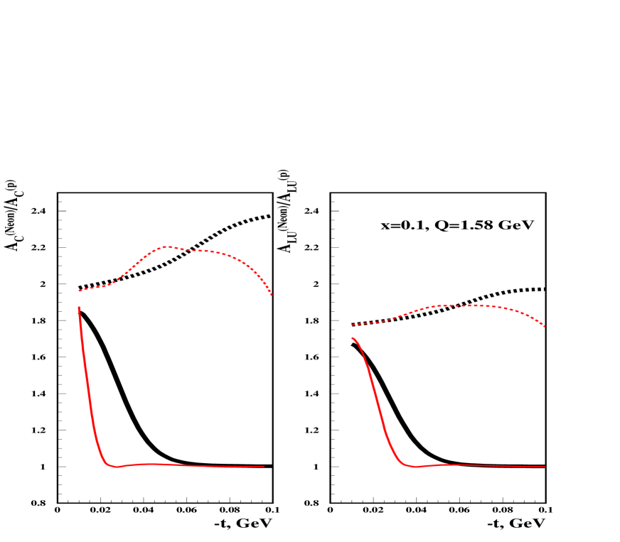
Figure 2: The ratio of nuclear to proton asymmetries $A_{C}/A_{C}^{{\rm proton}}$ and $A_{LU}/A_{LU}^{{\rm proton}}$ for Neon (thick black) and Krypton (thin red).

In order to illustrate these points, we consider DVCS on spinless nuclei of Neon ($A=20$ and $Z=10$) and Krypton (spinless isotope with $A=76$ and $Z=36$). Figure 2 presents the ratio of the nuclear to proton asymmetries, $A_{C}/A_{C}^{{\rm proton}}$ and $A_{LU}/A_{LU}^{{\rm proton}}$, as a function of $t$ at $x=0.1$ and $Q^{2}=2.5$ GeV² and fixed $\cos(\phi)$. This choice of $x$ and $Q^{2}$ roughly corresponds to the kinematics of the HERMES DVCS experiment with nuclei [8]. The solid curves is the full result including both incoherent and coherent contributions; the dashed curves include only the coherent part of the cross section. The following two features of Fig. 2 are of interest. Firstly, the ratio of the asymmetries for the coherent contribution (dashed curves) is significantly larger than unity. This is expected from the approximate expressions of Eqs. (31) and (35). As discussed above, an additional $t$-dependent enhancement arises because the bound nucleon GPDs, which enter the complete expressions of Eqs. (24) and (25), are probed at smaller values of $\xi$ than for the free proton.

Secondly, the inclusion of the incoherent contribution significantly reduces the ratio of the asymmetries (solid curves), especially at larger values of $|t|$, where the coherent contribution is suppressed by the smallness of the nuclear form factor. From the practical point of view, this means that if the experimental resolution in $t$ is poor, the asymmetries extracted from the experiment are obtained from the $t$-averaged data. This means for Eqs. (36) and (37) that first one integrates separately the nominator and denominator over $t$ and only then the ratio is taken. Integrating the nominators and denominators of $A_{C}$, $A_{LU}$, $A_{C}^{{\rm proton}}$ and $A_{LU}^{{\rm proton}}$ over $|t|$ from $|t|_{{\rm min}}=x_{Bj}m_{N}/(1-x_{Bj}+x_{Bj}m_{N}^{2}/Q^{2})$ to $|t|_{{\rm max}}=0.1$ GeV for Neon (the maximal $|t|$ measured by HERMES [8]) and to $|t|_{{\rm max}}=0.05$ GeV for Krypton (the coherent contribution for Krypton occupies a smaller $t$-range), and then taking the ratio of the nuclear to proton asymmetries, we obtain for Neon

$$\frac{\langle A_{C}(\phi,t)\rangle}{\langle A_{C}^{{\rm proton}}(\phi,t)\rangle}=1.10\pm 0.01\,,$$

$$\frac{\langle A_{LU}(\phi,t)\rangle}{\langle A_{LU}^{{\rm proton}}(\phi,t)\rangle}=1.05\pm 0.01\,,$$ (38)

and for Krypton

$$\frac{\langle A_{C}(\phi,t)\rangle}{\langle A_{C}^{{\rm proton}}(\phi,t)\rangle}=1.27\pm 0.01\,,$$

$$\frac{\langle A_{LU}(\phi,t)\rangle}{\langle A_{LU}^{{\rm proton}}(\phi,t)\rangle}=1.18\pm 0.01\,,$$ (39)

where

$$\langle A_{C}(\phi,t)\rangle=-\cos(\phi)\frac{8(2-2y+y^{2})x_{Bj}}{yc_{0}^{BH}}$$

$$\times\frac{\int^{|t|_{{\rm max}}}_{|t|_{{\rm min}}}d|t|K\int^{1}_{-1}dx\Big{(}P(\frac{1}{x-\xi})+P(\frac{1}{x+\xi})\Big{)}\Big{(}ZH^{p}(x,\xi,t)+Z(A-1)F_{A}^{e.m.}(t^{\prime})H_{A}(x,\xi,t^{\prime})\Big{)}}{\int^{|t|_{{\rm max}}}_{|t|_{{\rm min}}}d|t|\Big{(}ZF_{1}(t)+Z(Z-1)(F_{A}^{e.m.}(t^{\prime}))^{2}\Big{)}}\,,$$

$$\langle A_{C}^{{\rm proton}}(\phi,t)\rangle=-\cos(\phi)\frac{8(2-2y+y^{2})x_{Bj}}{yc_{0}^{BH}}$$

$$\times\frac{\int^{|t|_{{\rm max}}}_{|t|_{{\rm min}}}d|t|K\int^{1}_{-1}dx\Big{(}P(\frac{1}{x-\xi})+P(\frac{1}{x+\xi})\Big{)}H^{p}(x,\xi,t)}{\int^{0.1}_{|t|_{{\rm min}}}d|t|ZF_{1}(t)}\,.$$ (40)

The quantity $\langle A_{LU}(\phi,t)\rangle$ is defined similarly to $\langle A_{C}(\phi,t)\rangle$ with evident substitutions.

In order to carry out the above numerical analysis, we used a double distribution parametrization for the GPDs $H^{u}$ and $H^{d}$ without the D-term

$$H^{q}(x,\xi)=\int^{1}_{-1}d\beta\int^{1-|\beta|}_{-1+|\beta|}d\alpha\delta(x-\beta-\alpha\xi)h(\beta,\alpha)q(\beta)\,,$$ (41)

with $h(\beta,\alpha)=0.75((1-|\beta|)^{2}-\alpha^{2})/(1-|\beta|)^{3}$ [6] and $q(\beta)$ the parton density of the $u$ or $d$ quark. The parametrization for $q(\beta)$ is taken as that given by the CTEQ5M fit [16]. The $t$-dependence is chosen as in Ref. [6]: $H^{u}(x,\xi,t)=H^{u}(x,\xi)F_{1}(t)$, $H^{d}(x,\xi,t)=H^{d}(x,\xi)F_{1}(t)$ and $H^{s}(x,\xi,t)=0$, where $F_{1}(t)$ is the elastic form factor of the proton. This form factor is parametrized in a dipole form

$$F_{1}(t)=\frac{1}{(1+|t|/(0.71\,{\rm GeV}^{2})^{2}}\,.$$ (42)

The $t$-dependence of the nuclear GPD $H_{A}(x,\xi,t)$ is given by Eq. (23). The theoretical error included in Eqs. (38) and (39) reflects the uncertainty in the $t$-factorization ansatz for $H^{q}(x,\xi,t)$ and the uncertainty in the slope of the $t$-dependence of the elementary $\gamma^{\ast}N$ amplitude. The error was assessed by the modification $F_{1}(t)\to F_{1}(t)\exp(-2t)$: The answer for the ratios in Eqs. (38) and (39) changes very insignificantly.

The nuclear form factor is obtained as a Fourier transform of the nuclear density in the coordinate space

$$\rho_{A}(r)=\frac{\rho_{0}}{1+\exp((r-c)/z)}\,,$$ (43)

where $\rho_{0}=0.0081124$ fm^-3, $c=2.740$ fm and $z=0.572$ fm for Neon; $\rho_{0}=0.0020925$ fm^-3, $c=4.649$ fm and $z=0.545$ fm for Krypton [17].

5 Conclusions

The nuclear effect of Fermi motion in DVCS on spinless nuclear targets is considered within the framework of the impulse approximation. The amplitude of nuclear DVCS is expressed in terms of the convolution of the GPDs of the nucleons with the non-relativistic nuclear wave function.

The expressions for the beam-charge and single spin asymmetries in the HERMES kinematics are discussed extensively. It is shown that, apart from the combinatoric enhancement of the asymmetries because of the neutron contribution (see Eqs. (29) and (34), there are two additional effects: while Fermi motion of the nucleons enhances the asymmetries, the presence of the incoherent scattering at $t\neq 0$ drastically reduces the asymmetries.

References

• [1] HERMES Collab., A. Airapetian at al., Phys. Rev. Lett. 87 (2001) 182001.
• [2] ZEUS Collab., Measurement of the deeply virtual Compton scattering cross section at HERA, abstract 564, Intern. Europhys. Conf. on High Energy Physics, Budapest, Hungary, July 12.18, 2001.
• [3] H1 Collab., C. Adloff at al., Phys. Lett. B 517 (2001) 47.
• [4] CLAS Collab., S. Stepanyan at al., Phys. Rev. Lett. 87 (2001) 182002.
• [5] A.V. Belitsky, D. Müller and A. Kirchner, Theory of deeply virtual Compton scattering on the nucleon, preprint hep-ph/0112108, v2.
• [6] K. Goeke, M.V. Polyakov and M. Vanderhaeghen, Prog. Part. Nucl. Phys. 47 (2001) 401.
• [7] P.A.M. Guichon and M. Vanderhaeghen, Prog. Part. Nucl. Phys. 41 (1998) 125.
• [8] F. Ellinghaus, R. Shanidze and J. Volmer, Deeply-Virtual Compton Scattering on Deuterium and Neon at HERMES, preprint hep-ex/0212019.
• [9] M.V. Polyakov, Generalized parton distributions and strong forces inside nucleons and nuclei, preprint hep-ph/0210165.
• [10] F. Cano and B. Pire, Nucl. Phys. A711 (2002) 133; F. Cano and B. Pire, Deeply Virtual Compton Scattering on Spin-1 Nuclei, preprint hep-ph/0211444.
• [11] L.L. Frankfurt and M.I. Strikman, Phys. Rep.76 (1981) 215.
• [12] M. Sargsian, Int. J. Mod. Phys. E10 (2001) 405.
• [13] G.A. Miller, Prog. Part. Nucl. Phys. 45 (2000) 83.
• [14] A.V. Belitsky, D. Müller, A. Kirchner and A. Schäfer, Phys. Rev. D 64 (2001) 116002.
• [15] L. Frankfurt, G.A. Miller and M. Strikman, Phys. Rev. D 65 (2002) 094015.
• [16] H. Lai at al., Eur. Phys. J. C 12 (2000) 375.
• [17] H. De Vries, C.W. De Jager and C. De Vries, At. Data Nucl. Data Tables, 36 (1987) 495.