A Kinematically Complete Measurement of the Proton Structure Function $\mathbf{F}_{2}$ in the Resonance Region and Evaluation of Its Moments

Abstract

We measured the inclusive electron-proton cross section in the nucleon resonance region ($W<2.5$ GeV) at momentum transfers $Q^{2}$ below $4.5$ (GeV/c)² with the CLAS detector. The large acceptance of CLAS allowed the measurement of the cross section in a large, contiguous two-dimensional range of $Q^{2}$ and $x$, making it possible to perform an integration of the data at fixed $Q^{2}$ over the significant $x$-interval. From these data we extracted the structure function $F_{2}$ and, by including other world data, we studied the $Q^{2}$ evolution of its moments, $M_{n}(Q^{2})$, in order to estimate higher twist contributions. The small statistical and systematic uncertainties of the CLAS data allow a precise extraction of the higher twists and will require significant improvements in theoretical predictions if a meaningful comparison with these new experimental results is to be made.

I Introduction

The striking features of the nucleon structure function $F_{2}$ were first noted nearly 30 years ago by Bloom and Gilman BloGil. They empirically observed two effects in data measured at SLAC: a) the dual behaviour of the $F_{2}(x,Q^{2})$ function that shows common features between the two kinematic regions corresponding to the nucleon resonances and Deep Inelastic Scattering (DIS), b) the extension of the scaling region to lower $Q^{2}$ values when $F_{2}(x^{\prime},Q^{2})$ is plotted as a function of $x^{\prime}=x/(1+M^{2}x^{2}/Q^{2})$, the “improved scaling variable”. More precisely, they found that the smooth function $F_{2}(x^{\prime})$ measured at high $Q^{2}$ in the DIS region represents a good average over the resonances of the $F_{2}(x^{\prime},Q^{2})$ structure function measured at lower $Q^{2}$ values. Moreover, the duality appears to be valid locally. In fact, each of the most prominent resonance bumps, when averaged within its width, shows approximate scaling f2mom-hc . Later on, in the framework of QCD, De Rujula, Georgi and Politzer Rujula provided the first explanation of the Bloom-Gilman duality. They evaluated the Cornwall-Norton Corn-Nort moments $M_{n}^{CN}(Q^{2})$ of the nucleon structure function $F_{2}$, defined as

$$M^{CN}_{n}(Q^{2})=\int_{0}^{1}dxx^{(n-2)}F_{2}(x,Q^{2}),$$ (1)

using the Operator Product Expansion (OPE) they obtained the following expression

$$M^{CN}_{n}(Q^{2})=A_{n}(Q^{2})+\sum_{k=1}^{\infty}\biggl{(}n\frac{\gamma^{2}}{Q^{2}}\biggr{)}^{k}B_{nk}(Q^{2}),$$ (2)

where $A_{n}(Q^{2})$ can be evaluated in the framework of perturbative QCD (pQCD), and it is directly connected to the corresponding moment of the asymptotic limit of $F_{2}$. The contribution of the higher twists, which is related to multi-parton correlations inside the nucleon and represented by $B_{nk}(Q^{2})$, depends on the value of the constant $\gamma^{2}$ in such a way that $\gamma^{2}$ can be considered as a scale constant for higher twist effects. Assuming a small value of the constant $\gamma^{2}$, the authors of Ref. Rujula showed that the contribution of the higher twists was relatively small, at least for low values of $n$ and for $Q^{2}\geq M^{2}$, justifying the observed dual behaviour of the structure function.

It is now well established that the interpretation of the parton-hadron duality in light of QCD requires the evaluation of the moments of the nucleon structure functions and their evolution as a function of $Q^{2}$. Current pQCD calculations can estimate the $Q^{2}$ evolution up to the Next-to-Next-to-Leading Order, giving access to the interesting kinematic region of high $x$ and moderate $Q^{2}$ where the multi-parton correlation contribution to the nucleon wave function becomes dominant.

The interest in investigating multi-parton correlations in inelastic lepton scattering off the nucleon at large values of $x$ has recently been renewed, leading to a re-analysis of old $F_{2}$ data Ricco2 ; Nichtw . Unfortunately, the results from Ref. Ricco2 and Nichtw were mainly based on the analysis of fits of the structure function $F_{2}$ and therefore were still qualitative. Moreover, the previous lack of data in the resonance region did not allow a model independent evaluation of the moments’ evolution to lower $Q^{2}$, and therefore offered very few opportunities to quantitatively investigate the role of QCD below the DIS limit.

The Hall C Collaboration at the Thomas Jefferson National Accelerator Facility (TJNAF) has recently provided high quality data in this kinematic region f2-hc , allowing a more precise evaluation of the moments of the $F_{2}$ structure function of the proton f2mom-hc . However, like many other such measurements, the data were taken with a spectrometer of relatively small angular acceptance and the measured inclusive cross sections do not span a large continuous $x$ interval for constant $Q^{2}$. Data taken in this manner follow a kinematic locus in $Q^{2}$ vs. $x$ and require substantial interpolation to determine the $F_{2}$ moments.

Figure 1: Experimental data on the structure function $F_{2}(x,Q^{2})$ used for the moment evaluation in the CLAS kinematic region: points - world data; shaded area - CLAS data.

In this paper we report the first measurement in a wide continuous interval in $x$ and $Q^{2}$ (see Fig. 1) of the inclusive electron-proton scattering cross section. These measurements were performed at TJNAF with the CLAS detector in Hall B. The $F_{2}$ structure function was extracted over the whole resonance region ($W\leq 2.5$ GeV) below $Q^{2}=4.5$ (GeV/c)². This measurement, together with existing world data, allowed for the evaluation of the $F_{2}$ moments, drastically reducing the uncertainties related to data interpolation and providing the most detailed dependence on $Q^{2}$ of the moments up to $n=8$. Furthermore, the elastic contribution to the moments was updated with respect to Ref. Ricco2 using the fit of the nucleon form factors from Ref. Bosted adjusted to the Jefferson Lab data on the ratio $G_{E}/G_{M}$ hall-a , as described in Ref. CLAS_note . Finally, we used our new determination of the $F_{2}$ moments to extract the higher twist contribution as a function of $Q^{2}$.

In section II we review the $F_{2}$ moments in the framework of pQCD. In section III we discuss the analysis of the data, including the extraction of the $F_{2}$ structure function from the cross section. The evaluation of the moments and uncertainties is also presented in section III. Finally, Section IV is devoted to the interpretation of the results.

II Moments of the Structure Function $F_{2}$

Until recently the studies of inclusive lepton-nucleon scattering represented the main source of information about nucleon structure. In the DIS region, measured structure functions can be directly connected to the parton momentum distribution of the nucleon in the framework of pQCD. After the successful interpretation of the DIS region, the intermediate kinematic domain, situated at $Q^{2}$ of a few (GeV/c)² and large values of $x$, attracted the interest of physicists. Despite interpretation difficulties, this region allows the study of multi-parton correlation contribution to the proton wave function. These processes are not accessible in DIS due to the small value of the running coupling constant $\alpha_{S}(Q^{2})$.

The OPE of the virtual photon-nucleon scattering amplitude leads to the description of the complete $Q^{2}$ evolution of the moments of the nucleon structure functions. The n-th Cornwall-Norton moment Corn-Nort of the (asymptotic) structure function $F_{2}(x,Q^{2})$ for a massless nucleon can be expanded as:

$$M^{CN}_{n}(Q^{2})=\sum_{\tau=2k}^{\infty}E_{n\tau}(\mu,Q^{2})O_{n\tau}(\mu)\biggl{(}\frac{\mu^{2}}{Q^{2}}\biggr{)}^{{1\over 2}(\tau-2)},$$ (3)

where $k=1,2,...,\infty$, $\mu$ is the factorization scale, $O_{n\tau}(\mu)$ is the reduced matrix element of the local operators with definite spin $n$ and twist $\tau$ (dimension minus spin), related to the non-perturbative structure of the target. $E_{n\tau}(\mu,Q^{2})$ is a dimensionless coefficient function describing the small distance behaviour, which can be perturbatively expressed as a power expansion of the running coupling constant $\alpha_{s}(Q^{2})$.

At $Q^{2}$ values comparable with the squared proton mass, $M^{2}$, the structure function $F_{2}$ still contains non-negligible mass-dependent terms that produce in Eq. 3 additional $M^{2}/Q^{2}$ power corrections (kinematic twists). To avoid these terms, the moments $M^{CN}_{n}(Q^{2})$ of the massless $F_{2}$ have to be replaced in Eq. 3 by the corresponding Nachtmann Nachtmann moments $M^{N}_{n}(Q^{2})$ of the measured structure function $F_{2}(x,Q^{2})$ (see also Ref. Roberts ), It has been shown that:

$$M^{CN}_{n}\bigl{(}F^{lim}_{2}(x,Q^{2})\bigr{)}=M^{N}_{n}\bigl{(}F_{2}(x,Q^{2})\bigr{)},$$ (4)

where $F^{lim}_{2}(x,Q^{2})$ is the asymptotic structure function of the massless nucleon and

$$M^{N}_{n}(Q^{2})= \int_{0}^{1}dx\frac{\xi^{n+1}}{x^{3}}F_{2}(x,Q^{2})$$ (5)

$$\Biggl{[}\frac{3+3(n+1)r+n(n+2)r^{2}}{(n+2)(n+3)}\Biggr{]},$$

where $r=\sqrt{1+4M^{2}x^{2}/Q^{2}}$ and $\xi=2x/(1+r)$.

Since the moments in Eq. 3 are totally inclusive, the elastic contribution at $x=1$ has to be added according to Ref. f2mom-hc :

$$F^{el}_{2}(x,Q^{2})=\delta(1-x)\frac{\bigl{(}G_{E}^{2}(Q^{2})+\frac{Q^{2}}{4M^{2}}G_{M}^{2}(Q^{2})\bigr{)}}{\bigl{(}1+\frac{Q^{2}}{4M^{2}}\bigr{)}},$$ (6)

with $G_{E}^{2}$ $(G_{M}^{2})$ being the proton electric (magnetic) elastic form factor.

For the leading $\tau=2$ twist, one ends up in Leading Order (LO) or Next-to-Leading Order (NLO) with the well known perturbative logarithmic $Q^{2}$ evolution of singlet and non-singlet $F_{2}$ moments. However, if one wants to extend the analysis to small $Q^{2}$ and large $x$ where the rest of the perturbative series becomes significant, some procedure for the summation of the higher orders of the pQCD expansion, such as the infrared renormalon model renormalon ; Ricco1 or the recently developed soft-gluon resummation technique SGR ; SIM00 , has to be applied. For higher twists, $\tau>2$, the power terms $E_{n\tau}(\mu)$ are related to quark-quark and quark-gluon correlations, as illustrated by Fig. 2, and should become important at small $Q^{2}$.

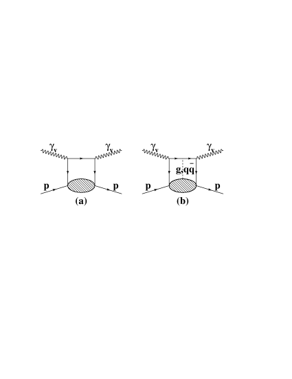
Figure 2: Twist diagrams:(a) the leading twist contribution evaluated at leading order of pQCD; (b) the contribution of higher twists, where current quark and nucleon remnant can exchange by a system of particles consisting of gluons and $q\bar{q}$-pairs whose complexity is increasing with twist order.

The systematic analysis of the $Q^{2}$ dependence of the experimentally derived Nachtmann moments $M^{N}_{n}(Q^{2})$ in the intermediate $Q^{2}$ range ($0.5<Q^{2}<10$ (GeV/c)²) should allow a separation of the higher twists from the leading twist. A precise evaluation would permit a comparison with the QCD predictions obtained from lattice simulations or a comparison with those models that describe the non-perturbative domain.

III Data Analysis

The data were collected at TJNAF in Hall B with the CLAS detector and a liquid hydrogen target with thickness $\rho x=0.35$ g/cm² during the electron beam running period in February-March 1999. The average beam current of 4.5 nA corresponded to a luminosity of 6x10³³ cm^-2s^-1. To cover the largest interval in $Q^{2}$ and $x$, data were taken at five different electron beam energies: $E_{0}=$ 1.5, 2.5, 4.0, 4.2 and 4.4 GeV. The CLAS detector is a magnetic spectrometer based on a six-coil torus magnet whose field is primarily oriented along the azimuthal direction. The sectors, located between the magnet coils, are instrumented individually to form six essentially independent magnetic spectrometers. The particle detection system includes drift chambers (DC) for track reconstruction dc , scintillation counters (TOF) for the time of flight measurement sc , Cherenkov counters (CC) for electron identification cc , and electromagnetic calorimeters (EC) to measure neutrals and to improve the electron-pion separation ec . The EC detectors have a granularity defined by triangular cells in the plane perpendicular to the incoming particles to study the electromagnetic shower shape and are longitudinally divided into two parts with the inner part acting as a pre-shower. Charged particles can be detected and identified for momenta down to 0.2 GeV/c and for polar angles between 8^∘ and 142^∘. The CLAS superconducting coils reduce the acceptance of about 80% at $\theta=90^{\circ}$ to about 50% at forward angles ($\theta=20^{\circ}$), while the total acceptance for electrons is about 1.5 sr. Electron momentum resolution is a function of the scattered electron angle and it varies from 0.5% for $\theta\leq 30^{\circ}$ up to 1-2% for $\theta>30^{\circ}$. The angular resolution is approximately constant and approaching 1 mrad for polar and 4 mrad for azimuthal angles: the resolution on the momentum transfer ranges therefore from 0.2 up to 0.5 %. The missing mass resolution was estimated 2.5 MeV for beam energy less than 3 GeV and about 7 MeV for larger energies. To study all possible multi-particle production, the acquisition trigger was configured to require at least one electron candidate in any of the sectors, where an electron candidate was defined as the coincidence of a signal in the EC and Cherenkov modules for each sector separately.

The accumulated statistics at the five energies is large enough ($>6\times 10^{8}$ triggers) to allow the extraction of the inclusive cross section with a rather small statistical error ($\leq 5$%), in small $x$ and $Q^{2}$ bins ($\Delta x=0.009$, $\Delta Q^{2}=0.05$ GeV²). The determination of the systematic error was more critical. CLAS is a large acceptance spectrometer and the response depends on the energy $E^{\prime}$ and the angle $\theta$ of the scattered electron. Determining the systematic effects of these, and other experimental parameters, is both necessary and complex. Consequently, we dedicate the next subsections to the discussion of the analysis procedure.

III.1 Momentum Correction

Determining the momentum of a charged particle measured with CLAS depends on a proper understanding of the magnetic field geometry. Due to the complexity of the detector and particularly the torus magnet system, it is crucial to check the reliability of the momentum determined by the DC tracking system. For this reason the position of the elastic peak was extracted from the measured inclusive electron cross section and compared to the theoretical value. A correction to the scattered electron momentum was applied to shift the elastic peak to the accepted value. The momentum correction obtained was small (from 2 to 7 MeV in $W$, depending on the beam energy) and resulted in significant improvement in the width of elastic peak .

The systematic error on the correction was estimated by comparing the position of the well known second resonance ($S_{11}(1535)+D_{13}(1520)$) to the position given in Ref. Bodek ; Stein . The position difference $\Delta W$ affects the cross section evaluation. The relative systematic error on the momentum correction is therefore given by

$$\delta_{mom}(x,Q^{2})=\frac{|\sigma^{B}(W-\frac{\Delta W}{2},Q^{2})-\sigma^{B}(W+\frac{\Delta W}{2},Q^{2})|}{\sigma^{B}(W,Q^{2})}~{},~{}~{}~{}~{}$$ (7)

where $\sigma^{B}$ represents the Bodek fit according to the parametrization from Ref. Bodek ; Stein . The systematic error calculated with Eq. 7 is given in Table. 1.

III.2 Electron Identification and Pion Rejection

The electrons were identified by a combined off-line analysis of the signals from the four detector systems (DC, TOF, CC and EC). Only those electron candidates that were detected inside the most uniform (“fiducial”) detector volume were analyzed. The electron yield was corrected separately in each kinematic bin, for pion contamination, detection efficiency and radiative corrections.

Figure 3: Photoelectron distribution in the Cherenkov detector versus the energy deposited in the EC detector divided by the momentum of the particle as determined by the drift chamber. The black vertical line represents the cut to reduce the pion contamination.

The photoelectron distribution in the CC depends on the kinematics, and the contaminating pion peak can be completely removed only with large efficiency losses of about 30% in several kinematic regions. Therefore the pion contamination was removed by a two-step procedure. Electrons producing a large number of photoelectrons (see Fig. 4) were identified by an energy cut in the EC detector response. The pion contamination to electrons producing a small number of photoelectrons was removed by analysis of the CC response.

As an example of the first step, Fig. 3 shows the CC photoelectron distribution $N_{phe}$ as a function of the fraction of energy deposited in the EC detector $EC_{tot}/P$ for negatively charged particles emitted at $\theta<35^{\circ}$, momentum $P<1$ GeV/c, and a beam energy of $2.5$ GeV. The regions corresponding to pions ($N_{phe}\leq 2.5$) and to electrons ($EC_{tot}/P\geq 0.25$) cannot be clearly separated and only the pion contamination to the left of the solid line can be removed without affecting the electron detection efficiency. The remaining pion contamination and the correction of the Cherenkov efficiency for electrons $F_{phe}$ have determined by a combined fit of the measured photoelectron distribution with two Poisson distributions convoluted with a Gaussian function to account for the finite photomultiplier resolution as shown in Fig. 4.

Figure 4: The fitted photoelectron distribution for two different sets of kinematics after removing some of the pion contamination via the $EC_{tot}/P$ cut: solid triangles show the distribution obtained with $4$ GeV beam, scattered electron angle $\theta=31^{\circ}$ and momentum $P=1$ GeV; empty diamonds represent data taken with $2.5$ GeV beam, scattered electron angle $\theta=41^{\circ}$ and momentum $P=1$ GeV.

The fit was performed separately for each sector over the whole kinematics data set ($\theta=20^{\circ}-50^{\circ}$ and $W=0.9-2.5$ GeV)

To minimize the errors, the fit was performed in rather large bins ($\Delta\theta=2^{\circ}$ and $\Delta E^{\prime}\sim 0.1$ GeV). Therefore, in order to apply the correction to the measured cross section, which was obtained with smaller bins, values of the correction were parametrized with the polynomial function:

$$F_{phe}(\nu,\theta)=1+A(\nu-\nu_{0})+(B+C\theta)(\nu-\nu_{0})^{2}~{},$$ (8)

where $A$, $B$, $C$ and $\nu_{0}$ are free parameters and $\nu=E_{0}-E^{\prime}$ the electron energy transfer. The related systematic error $\delta_{phe}=\delta{F_{phe}}/F_{phe}$ is mainly due to the low statistics in those bins corresponding to large $Q^{2}$ values and was found to be less than $2$%.

III.3 Background Subtraction

Since the pair production background has not been measured, its contribution was estimated according to a model BostedPP based on the Wiser fit Wiser of the inclusive pion photo-production reaction. The most important source of $e^{+}e^{-}$ pairs in the CLAS is due to $\pi^{0}$ production, which either decays to $\gamma e^{+}e^{-}$ (Dalitz decay) or to $\gamma\gamma$, with subsequent photon conversion to $e^{+}e^{-}$. The model was carefully checked, and it was in good agreement with the measured positron cross sections BostedPP ; the difference was always less than 30%. The value of the correction was assumed to be equal to the ratio of the inclusive $e^{+}$ production cross section $\sigma_{e^{+}}$ over Bodek’s fit Bodek ; Stein including radiative processes (tail from the elastic peak, bremsstrahlung, and Schwinger correction) $\sigma^{B}_{rad}$:

$$F_{e^{+}e^{-}}(E_{0},E^{\prime},\theta)=\frac{1}{1+\frac{\sigma_{e^{+}}(E_{0},E^{\prime},\theta)}{\sigma^{B}_{rad}(E_{0},E^{\prime},\theta)}}~{}.$$ (9)

The correction is generally small as expected in Ref. f2-hc , therefore it was applied only for $E_{0}>2.0$ GeV and $W>1.7$ GeV, where it was about 2%. The relative systematic error $\delta_{e^{+}e^{-}}=\delta{F_{e^{+}e^{-}}}/F_{e^{+}e^{-}}$ from this correction was estimated using uncertainties on $\sigma_{e^{+}}$ given in Ref. BostedPP .

In order to remove the contribution of scattering on the target walls, the empty target data were analyzed in the same way and subtracted from the inclusive data, after proper normalization. An additional source of background originating from knock-on electrons produced in the supporting structure of the detector was estimated and it found to be smaller than 0.3%.

III.4 Simulations

Due to the complexity of the CLAS detector the only way to study its response functions is to perform complete computer simulations, describing each subsystem in detail including all materials that make up each detector. The simulations of detector response to the scattered electron were performed according to the following procedure:

1. Electron scattering events were generated by a random event generator with the probability distributed according to $\sigma^{B}_{rad}$, described above. The values of elastic and inelastic cross sections of the electron-proton scattering were taken from existing fits of world data, in references Bosted and Bodek ; Stein , respectively. The internal radiative processes contribution was added according to calculations Mo .

2. The generated events were passed through the standard CLAS GEANT-based simulation program GSIM , to model the detector response.

3. The results of the previous stage were further processed to make the detector response more realistic by adding the effects of electronic noise, background, dead wires and scintillator paddles.

4. Finally, the efficiency was calculated in each kinematic bin as a ratio of the number of reconstructed events $N_{rec}$ over the number of generated events $N_{gen}$:

   $$\epsilon_{eff}(E_{0},x,Q^{2})=\frac{N_{rec}(E_{0},x,Q^{2})}{N_{gen}(E_{0},x,Q^{2})}~{}.$$ (10)

The electron detection efficiency obtained from simulations is about 97% and approximately constant inside the fiducial region of the detector over the whole available kinematics.

In order to test the reliability of the simulation procedure and to check a proper absolute normalization, the well known elastic scattering cross section was extracted from the same data set ($\frac{d\sigma}{d\Omega}_{exp}$) and compared to the simulated cross section ($\frac{d\sigma}{d\Omega}_{sim}$). The two cross sections are in good agreement within statistical and systematic errors as shown in Fig. 5.

Figure 5: Typical ratio of the measured elastic scattering cross section to the parametrization from Refs. Bosted ; hall-a (points) with radiative corrections, in comparison to that obtained from the simulations (continuous line); errors are statistical only.

The relative systematic deviation of the elastic cross section obtained from simulations and from these data $\delta_{eff}$, was calculated for each beam energy and scattered electron angle (in bins of one degree on the accessible interval from 20 to 50 degrees) according to:

$$\delta^{2}_{eff}(E_{0},\theta) + \delta^{2}_{exp}(E_{0},\theta)=$$ (11)

$$\Biggl{[}\frac{\frac{d\sigma}{d\Omega}_{exp}(E_{0},\theta)-\frac{d\sigma}{d\Omega}_{sim}(E_{0},\theta)}{\frac{d\sigma}{d\Omega}_{fit}(E_{0},\theta)}\Biggr{]}^{2}~{},~{}~{}~{}~{}~{}~{}$$

where $\frac{d\sigma}{d\Omega}_{fit}$ is the parametrization described in Ref. Bosted and $\delta_{exp}$ is the statistical error of the measured elastic cross section. For the error propagation $\delta_{eff}$ was parametrized by a linear function of the scattered electron angle $\theta$.

III.5 Inclusive Inelastic Cross Section

Since the Monte Carlo simulations were shown to be reliable, they were used to evaluate efficiency, acceptance, bin centering and radiative corrections. For each kinematic bin, the inclusive cross section $d\sigma$ and the structure function $F_{2}$ were extracted directly from the raw electron yield $N_{exp}$ normalized to the integrated luminosity and corrected for efficiency, acceptance, bin centering, and radiative effects as follows:

$$\frac{d^{2}\sigma}{dxdQ^{2}} = \frac{1}{\rho\frac{N_{A}}{M_{A}}LQ_{tot}}\frac{N_{exp}(x,Q^{2})}{\epsilon(x,Q^{2})}$$ (12)

$$F_{phe}(x,Q^{2})F_{e^{+}e^{-}}(x,Q^{2})~{},$$

where $\rho$ is the density of liquid $H_{2}$ in the target, $N_{A}$ is the Avogadro constant, $M_{A}$ is the target molar mass, $L$ is the target length, $Q_{tot}$ is the total charge in the Faraday Cup (FC) and $\epsilon(x,Q^{2})$ is the efficiency defined in Eq. 10 with the radiative and bin-centering correction factors according to:

$$\epsilon(x,Q^{2})=\epsilon_{eff}(x,Q^{2})\epsilon_{rad}(x,Q^{2})\epsilon_{bin}(x,Q^{2})~{},$$ (13)

where

$$\epsilon_{rad}=\frac{\sigma^{B}_{rad}}{\sigma^{B}}~{}~{}~{}\mbox{and}~{}~{}~{}\epsilon_{bin}=\frac{\int_{\Delta\tau}d\sigma^{B}}{\sigma^{B}}~{},$$ (14)

and the integral was taken over the current bin area $\Delta\tau$. The radiative correction factor $\epsilon_{rad}$ strongly varies in the explored kinematic range from 0.85 up to 1.6. Fortunately, the largest correction was contributed by the elastic peak tail for which calculations are very accurate (see Refs. Mo ; Akushevich ).

All systematic uncertainties were propagated in quadrature to the final relative systematic error:

$$\delta_{sys}(x,Q^{2})=\bigl{[}\delta_{eff}^{2}(x,Q^{2})+\delta_{phe}^{2}(x,Q^{2})+$$

$$\delta_{e^{+}e^{-}}^{2}(x,Q^{2})+\delta_{mom}^{2}(x,Q^{2})+\delta_{rad}^{2}(x,Q^{2})\bigr{]}^{1/2}~{},~{}$$ (15)

where $\delta_{rad}$ is the systematic uncertainty on the radiative correction, given by:

$$\delta_{rad}(E,x,Q^{2})=\Bigl{|}\epsilon^{TSAI}_{rad}(E,x,Q^{2})-\epsilon^{POLRAD}_{rad}(E,x,Q^{2})\Bigr{|}~{},$$ (16)

where $\epsilon^{TSAI}_{rad}(E,x,Q^{2})$ and $\epsilon^{POLRAD}_{rad}(E,x,Q^{2})$ are the radiative correction factors in $\sigma^{B}_{rad}$ evaluated with two different approaches (Mo , Akushevich ). These two approaches use different parametrizations of the elastic (Bosted and Bilenka ) and inelastic (Bodek ; Stein and Brasse ) cross sections as well as different calculation techniques.

$\delta_{rad}(E,x,Q^{2})$ varies in the kinematic range of the experiment from 0 to 20% while the average value is 3%. A minimum radiative correction systematic error of 1.5% was assumed.

III.6 Structure Function $F_{2}(x,Q^{2})$

The structure function $F_{2}(x,Q^{2})$ was extracted from the inelastic cross section using the fit of the function $R(x,Q^{2})\equiv\sigma_{L}/\sigma_{T}$ developed in Ricco1 and described in Appendix A. The inclusive electron scattering cross section can be expressed in terms of the well known structure functions $W_{1}$ and $W_{2}$ as Roberts :

$$\frac{d^{2}\sigma}{d\Omega dE^{\prime}}=\sigma_{Mott}\bigl{\{}2W_{1}(x,Q^{2})\tan^{2}{\frac{\theta}{2}}+W_{2}(x,Q^{2})\bigr{\}}~{},$$ (17)

where the Mott cross section is given by:

$$\sigma_{Mott}=\frac{\alpha^{2}\cos^{2}{\frac{\theta}{2}}}{4E^{2}\sin^{4}{\frac{\theta}{2}}}~{}.$$ (18)

Therefore, the structure function $F_{2}=\nu W_{2}$ is given by:

$$F_{2}(x,Q^{2})=\frac{1}{\sigma_{Mott}}\frac{d^{2}\sigma}{dxdQ^{2}}J\frac{\nu}{1+\frac{1-\epsilon}{\epsilon}\frac{1}{1+R}}~{},$$ (19)

where $J$ is the Jacobian given by

$$J=\frac{x(s-M^{2})}{2\pi M\nu}E^{\prime}~{},$$ (20)

where $\it s$ is the squared invariant mass of the initial electron-proton system $s=M^{2}+2EM$ and $\epsilon$ is the polarization parameter defined as

$$\epsilon\equiv\Biggl{(}1+2\frac{\nu^{2}+Q^{2}}{Q^{2}}\tan^{2}{{\theta\over 2}}\Biggr{)}^{-1}~{}.$$ (21)

The function $R(x,Q^{2})$ is poorly known in the resonance region, however the structure function $F_{2}$ in the relevant kinematic range is very insensitive to the value of $R$. In fact even a 100% systematic uncertainty on $R$ gives only a few percent uncertainty on $F_{2}$. The relative total systematic error is given by:

$$\delta^{sys}_{F_{2}}(x,Q^{2})=\Biggl{[}\delta_{sys}^{2}(x,Q^{2})+\Biggl{(}\frac{1-\epsilon}{1+\epsilon R}\frac{\delta_{R}}{1+R}\Biggr{)}^{2}\Biggr{]}^{1/2}~{}.$$ (22)

The uncertainties of $R$ given in Ref. Ricco1 were propagated to the resulting $F_{2}$, and the actual systematic errors introduced by $\delta_{R}$ were always lower than 3%.

The combined statistical and systematic precision of the obtained structure function $F_{2}$ is strongly dependent on kinematics and the statistical errors vary from 0.2% up to 30% at the largest $Q^{2}$ where statistics are very limited. Fig. 6 shows a comparison between the $F_{2}$ data from CLAS and the other world data in the $Q^{2}=0.775$ GeV² bin. The observed discrepancies with the data from Ref. f2-hc which fill the large $x$ region in Fig. 6 are mostly within the systematic errors. Because of the much smaller bin centering corrections in this $Q^{2}$ region our data are in a better agreement with data previously measured at SLAC, given in Ref. Stein , and the parameterization of those from Ref. Bodek ; Stein . The average statistical uncertainty is about 5%; the systematic uncertainties range from 2.5% up to 30%, with the mean value estimated as 7.7% (see Table 1). The values of $F_{2}(x,Q^{2})$ determined using our data are tabulated elsewhere CLAS_note .

Table 1: Range and average of systematic errors on $F_{2}$.

Source of uncertainties	Variation range	Average
	[%]	[%]
Efficiency evaluation	1-9	4.3
$e^{+}e^{-}$ pair production correction	0-3	0.3
Photoelectron correction	0.1-2.2	0.6
Radiative correction	1.5-20	3.2
Momentum correction	0.1-30	3.5
Uncertainty of $R=\frac{\sigma_{L}}{\sigma_{T}}$	0.5-5	2.4
Total	2.5-30	7.7

Figure 6: Structure function $F_{2}(x,Q^{2})$ at $Q^{2}=0.775$ GeV²: stars represent experimental data obtained in the present analysis with systematic errors indicated by the hatched area, empty circles show data from previous experiments  f2-hc ; BCDMS ; E665 ; NMC ; H1a ; H1b ; H1c ; H1d ; H1e ; ZEUSa ; ZEUSb ; ZEUSc ; ZEUSd ; ZEUSe ; ZEUSf ; SLAC and the solid line represents the parametrization from Ref. Ricco1 .

III.7 Moments of the Structure Function $F_{2}$

As discussed in the introduction, the final goal of this analysis is the evaluation of the Nachtmann moments of the structure function $F_{2}$. The total Nachtmann moments were computed as the sum of the elastic and inelastic moments:

$$M_{n}=M^{el}_{n}+M^{in}_{n}~{}.$$ (23)

The contribution originating from the elastic peak was calculated according to the following expression from Ref. Ricco1 :

$$M^{el}_{n}=\biggl{(}\frac{2}{1+r}\biggr{)}^{n+1} \frac{3+3(n+1)r+n(n+2)r^{2}}{(n+2)(n+3)}$$ (24)

$$\frac{G_{E}^{2}(Q^{2})+\frac{Q^{2}}{4M^{2}}G_{M}^{2}(Q^{2})}{1+\frac{Q^{2}}{4M^{2}}}~{},$$

where the proton form factors $G_{E}^{2}(Q^{2})$ and $G_{M}^{2}(Q^{2})$ are from Ref. Bosted modified according the recently measured data on $G_{E}/G_{M}$ hall-a , as described in Ref. CLAS_note .

The evaluation of the inelastic moment $M^{in}_{n}$ involves the computation at fixed $Q^{2}$ of an integral over $x$. For this purpose, in addition to the results obtained from the CLAS data, world data on the structure function $F_{2}$ from Refs. f2-hc ; BCDMS ; E665 ; NMC ; H1a ; H1b ; H1c ; H1d ; H1e ; ZEUSa ; ZEUSb ; ZEUSc ; ZEUSd ; ZEUSe ; ZEUSf ; SLAC and data on the inelastic cross section csworld ; Bodek ; Stein were used to reach an adequate coverage (see Fig. 1). The integral over $x$ was performed numerically using the standard trapezoidal method TRAPER cernlib . Data from Ref. EMC were not included in the analysis due to their inconsistency with other data sets as explained in detail in Ref. disfit2 , and data from Ref. WA25 ; new-inclusive were not included due to the large experimental uncertainties.

The $Q^{2}$-range from 0.05 to 3.75 (GeV/c)² was divided into $\Delta Q^{2}=0.05$ (GeV/c)² bins. Then within each $Q^{2}$ bin the world data were shifted to the central bin value $Q^{2}_{0}$, using the fit of $F_{2}^{B}(x,Q^{2})$ from Ref. Ricco1 . Here the fit $F_{2}^{B}(x,Q^{2})$ consists of two parts, a parametrization Bodek ; Stein in the resonance region ($W<2.5$ GeV), and a QCD-like fit from Ref. disfit1 in the DIS ($W>2.5$ GeV):

$$F_{2}(x,Q^{2}_{0})=\frac{F_{2}(x,Q^{2})}{F_{2}^{B}(x,Q^{2})}F_{2}^{B}(x,Q^{2}_{0})~{}.$$ (25)

The difference between the real and bin-centered data

$$\delta^{cent}_{F_{2}}(x,Q^{2})=F_{2}(x,Q^{2})\Biggl{|}1-\frac{F^{B}_{2}(x,Q^{2}_{0})}{F_{2}^{B}(x,Q^{2})}\Biggr{|}~{}~{},$$ (26)

was added to the systematic errors of $F_{2}$ in extracting the Nachtmann moments. As an example, Fig. 7 shows the integrands of the first four moments as a function of $x$ at fixed $Q^{2}$. The significance of the large $x$ region for various moments can clearly be seen .

Figure 7: Integrands of the inelastic Nachtmann moments at $Q^{2}=0.825$ GeV²: circles represent the integrand of the $M_{2}$; squares show the integrand of the $M_{4}$; triangles - the integrand of the $M_{6}$; crosses - the integrand of the $M_{8}$.

To have a data set dense in $x$, which reduces the error in the numerical integration, we performed an interpolation, at each fixed $Q^{2}_{0}$, when two contiguous experimental data points differed by more than $\nabla$. The value of $\nabla$ depended on kinematics; in the resonance region where the structure function exhibits strong variations, $\nabla$ had to be smaller than half the resonance widths and was parametrized as $\nabla=0.04/\Bigl{[}1+\sqrt{Q^{2}/10}\Bigr{]}$. Above the resonances, where $F_{2}$ is smooth, we only accounted for the fact that the available $x$ region decreases with decreasing $Q^{2}$ ($\nabla=0.1\Bigl{[}1+\sqrt{Q^{2}/10}\Bigr{]}$). Finally in the low $x$ region ($x<0.03$) where the $F_{2}$ shape depends weakly on $Q^{2}$, but strongly on $x$, we set $\nabla=0.015$. Changing these $\nabla$ values by as much as a factor two produced changes in the moments that were much smaller than the systematic errors.

To fill the gap within two contiguous points $x_{a}$ and $x_{b}$, we used the interpolation function $F_{2}^{int}(x,Q^{2}_{0})$ defined as the parametrization from Ref. Ricco1 normalized to the experimental data on both edges of the interpolating range. Assuming that the shape of the fit is correct:

$$F_{2}^{int}(x,Q^{2}_{0})=\alpha(Q^{2}_{0})F_{2}^{B}(x,Q^{2}_{0})~{},$$ (27)

where the normalization factor $\alpha(Q^{2}_{0})$ is defined as the weighted average, evaluated using all experimental points located within an interval $\Delta$ around $x_{a}$ or $x_{b}$:

$$\alpha(Q^{2}_{0})=\delta_{N}^{2}(Q^{2}_{0})\Biggl{[}\sum\limits_{i}^{|x_{i}-x_{a}|<\Delta}\frac{F_{2}(x_{i},Q^{2}_{0})/F_{2}^{B}(x_{i},Q^{2}_{0})}{\bigl{(}\delta_{F_{2}}^{stat}(x_{i},Q^{2}_{0})\bigr{)}^{2}}+$$

$$\sum\limits_{j}^{|x_{j}-x_{b}|<\Delta}\frac{F_{2}(x_{j},Q^{2}_{0})/F_{2}^{B}(x_{j},Q^{2}_{0})}{\bigl{(}\delta_{F_{2}}^{stat}(x_{j},Q^{2}_{0})\bigr{)}^{2}}\Biggr{]}~{},$$ (28)

where $\delta_{F_{2}}^{stat}(x_{j},Q^{2}_{0})$ is the statistical error relative to $F_{2}^{B}$ and

$$\delta_{N}(Q^{2}_{0})=\Biggl{[}\sum\limits_{i}^{|x_{i}-x_{a}|<\Delta}\frac{1}{\bigl{(}\delta_{F_{2}}^{stat}(x_{i},Q^{2}_{0})\bigr{)}^{2}}+$$

$$\sum\limits_{j}^{|x_{j}-x_{b}|<\Delta}\frac{1}{\bigl{(}\delta_{F_{2}}^{stat}(x_{j},Q^{2}_{0})\bigr{)}^{2}}\Biggr{]}^{-1/2}~{},$$ (29)

is the statistical uncertainty of the normalization. Therefore, the statistical error of the moments calculated according the trapezoidal rule cernlib was increased by adding the linearly correlated contribution from each interpolation interval as follows:

$$\delta^{norm}_{n}(Q^{2}_{0})= \delta_{N} (Q^{2}_{0})\int\limits_{x_{a}}^{x_{b}}dx\frac{\xi^{n+1}}{x^{3}}F_{2}^{B}(x,Q^{2}_{0})$$ (30)

$$\frac{3+3(n+1)r+n(n+2)r^{2}}{(n+2)(n+3)}~{}.$$

Since we average the ratio $F_{2}(x_{i},Q^{2}_{0})/F_{2}^{B}(x_{i},Q^{2}_{0})$, $\Delta$ is not affected by the resonance structures, and its value was fixed to have more than two experimental points in most cases; therefore, $\Delta$ was chosen equal to 0.03 in the resonance and in the very low $x$ regions, and to 0.05 in the DIS region. In Fig. 8 we show how this interpolation is applied: the thin continuous line represents the original function $F_{2}^{B}(x,Q^{2})$ and the heavy continuous line represents the result of the interpolation $F_{2}^{int}(x,Q^{2})$. We also checked that the moments do not show any dependence on the $\Delta$ values.

Figure 8: Example of the interpolating procedure. The meaning of the curves and symbols is described in the text.

To fill the gap between the last experimental point and one of the integration limits ($x_{a}=0$ or $x_{b}=1$) we performed an extrapolation at each fixed $Q^{2}_{0}$ using $F_{2}^{B}(x,Q^{2}_{0})$ including its systematic error given in Ref. Ricco1 .

As an extension of the analysis, the world data at $Q^{2}$ above $5$ (GeV/c)² were analyzed in the same way as described above. The only differences were the $Q^{2}$ bin size, which was chosen equal to 5% of $Q^{2}$, and the values of the parameters $\nabla$ and $\Delta$. In addition, the bins were situated not continuously, but only where data exist. Since at large $Q^{2}$ the shape of $F_{2}(x)$ remains almost constant with changing $Q^{2}$ both parameters $\nabla$ and $\Delta$ were fixed: in the resonance region ($W<1.8$ GeV) to value $0.01$; $0.1$ in the DIS; and $\nabla=0.005$ and $\Delta=0.01$ at very low $x$ ($x<0.03$). The results for $M^{in}_{n}(Q^{2})$ did not exhibit any significant dependence on the choice of the parameter values. The results are reported together with their statistical and systematic errors in Table 2.

III.8 Systematic Errors of the Moments

The systematic error consists of genuine uncertainties in the data given in Refs. f2-hc ; BCDMS ; E665 ; NMC ; H1a ; H1b ; H1c ; H1d ; H1e ; ZEUSa ; ZEUSb ; ZEUSc ; ZEUSd ; ZEUSe ; ZEUSf ; SLAC ; Bodek ; Stein ; csworld and uncertainties in the evaluation procedure. To estimate the first type of error we had to account for using many data sets measured, in different laboratories, and with different detectors. In the present analysis we assume that different experiments are independent and therefore only systematic errors within one data set are correlated.

Thus, an upper limit for the contribution of the systematic error from each data set was evaluated in the following way:

• we first applied a simultaneous shift to all experimental points in this set by an amount equal to their systematic error;

• then the inelastic $n$-th moments obtained using these distorted data $\tilde{M}^{in}_{n(i)}(Q^{2})$ were compared to the original moments $M^{in}_{n}(Q^{2})$ evaluated with no systematic shifts;

• finally the deviations for each data set were summed in quadrature as independent values:

  $$\delta_{n}^{D}(Q^{2})=\frac{1}{M^{in}_{n}(Q^{2})}\sqrt{\sum\limits_{i}^{N_{S}}\Bigl{(}\tilde{M}^{in}_{n(i)}(Q^{2})-M^{in}_{n}(Q^{2})\Bigr{)}^{2}}~{},$$ (31)

  where $N_{S}$ is the number of available data sets. The resulting error was summed in quadrature to $\delta_{n}^{norm}(Q^{2})$ to finally evaluate the total systematic error of the $n$-th moment.

The second type of error is related to the bin centering, interpolation and extrapolation. The bin centering systematic uncertainty was estimated as follows:

$$\delta^{C}_{n}(Q^{2})=\sum_{i}K_{n}(x_{i},Q^{2})w_{i}(Q^{2})\delta^{cent}_{F_{2}}(x_{i},Q^{2})~{},$$ (32)

where according the Nachtmann moment definition and the trapezoidal integration rule:

$$K_{n}(x_{i},Q^{2}) = \frac{\xi_{i}^{n+1}}{x_{i}^{3}}\frac{3+3(n+1)r_{i}+n(n+2)r_{i}^{2}}{(n+2)(n+3)}$$

$$w_{i}(Q^{2}) = (x_{i+1}-x_{i-1})/2~{}.$$ (33)

The relative systematic error of the interpolation was estimated as the possible change of the fitting function slope in the interpolation interval, and it was evaluated as a difference in the normalization at different edges:

$$\delta_{S}(Q^{2}_{0})=\Biggl{|}\frac{1}{N_{i}}\sum\limits_{i}^{|x_{i}-x_{a}|<\Delta}\frac{F_{2}(x_{i},Q^{2}_{0})}{F_{2}^{B}(x_{i},Q^{2}_{0})}-$$

$$\frac{1}{N_{j}}\sum\limits_{j}^{|x_{j}-x_{b}|<\Delta}\frac{F_{2}(x_{j},Q^{2}_{0})}{F_{2}^{B}(x_{j},Q^{2}_{0})}\Biggr{|}~{},$$ (34)

where $N_{i}$ and $N_{j}$ are the number of points used to evaluate the sums. Since the structure function $F_{2}(x,Q^{2})$ is a very smooth function of $x$ below resonances, on the limited $x$-interval (smaller than $\nabla$) the linear approximation gives a good estimate. Thus, the error given in Eq. 34 accounts for such a linear mismatch between the fitting function and the data on the interpolation interval. Meanwhile, the CLAS data cover all the resonance region and no interpolation was used there. Therefore, the total systematic error introduced in the corresponding moment by the interpolation can be estimated as

$$\delta^{I}_{n}(Q^{2}_{0})= \delta_{S} (Q^{2}_{0})\int\limits_{x_{a}}^{x_{b}}dx\frac{\xi^{n+1}}{x^{3}}F_{2}^{B}(x,Q^{2}_{0})$$ (35)

$$\frac{3+3(n+1)r+n(n+2)r^{2}}{(n+2)(n+3)}~{}.$$

The systematic errors obtained by these procedures were summed in quadrature:

$$\delta^{P}_{n}(Q^{2})=\sqrt{(\delta^{D}_{n}(Q^{2}))^{2}+(\delta^{C}_{n}(Q^{2}))^{2}+(\delta^{I}_{n}(Q^{2}))^{2}}~{}.$$ (36)

In order to study the systematic error on the extrapolation at very low $x$ we have performed a test of the functional form dependence comparing moments presented here with those obtained by using the fitting function from the neural network parametrization of Ref. Forte . The difference is significant only for $M_{2}$ and it appeared to be smaller than $\delta^{P}_{n}(Q^{2})$ given by Eq. 36 (see Fig. 9). The difference was added to $\delta^{P}_{n}(Q^{2})$ in quadrature to evaluate the total systematic error of the $n$-th moment.

Figure 9: Errors of the inelastic Nachtmann moment $M_{2}$ in percentage: empty circles represent statistical errors; empty crosses show the systematic error obtained in Eq. 36; the difference between inelastic moments extracted using two different $F_{2}$ parametrizations Ricco1 and Forte at $W>2.5$ GeV is shown by stars.

IV Extraction of leading and higher twists

In this Section, we present our twist analysis of the moments we have extracted, which are presented in Fig. 10. As already shown in Refs. Ricco1 and SIM00 , the extraction of higher twists at large $x$ depends significantly on the effects of pQCD high-order corrections. In particular, the use of the well established NLO approximation for the leading twist is known to lead to unreliable results for the higher twists SIM00 . Therefore, hereafter we follow Ref. SIM00 , where the pQCD corrections beyond the NLO are estimated according to soft gluon resummation (SGR) techniques.

Figure 10: The inelastic Nachtman moments extracted from the world data, including the new CLAS results, are shown as the solid shapes ; while the solid line represents moments obtained in Ref. Ricco1 . The empty crosses indicate the Nachtman moments determined in Ref. f2mom-hc . Errors are statistical only.

As far as power corrections are concerned, several higher-twist operators exist and mix under the renormalization-group equations. Such mixings are rather involved and the number of mixing operators increases with the order $n$ of the moment. Since a complete calculation of the higher-twist anomalous dimensions is not yet available, we use the same phenomenological ansatz already adopted in Refs. Ricco1 and SIM00 . Thus, our extracted Nachtmann moments are analyzed in terms of the following twist expansion

$$M_{n}^{N}(Q^{2})=\eta_{n}(Q^{2})+HT_{n}(Q^{2})~{},$$ (37)

where $\eta_{n}(Q^{2})$ is the leading twist moment and $HT_{n}(Q^{2})$ is the higher-twist contribution given by Ji

$$HT_{n}(Q^{2})= a_{n}^{(4)}\biggl{[}\frac{\alpha_{s}(Q^{2})}{\alpha_{s}(\mu^{2})}\biggr{]}^{\gamma_{n}^{(4)}}\frac{\mu^{2}}{Q^{2}}$$

$$+ a_{n}^{(6)}\biggl{[}\frac{\alpha_{s}(Q^{2})}{\alpha_{s}(\mu^{2})}\biggr{]}^{\gamma_{n}^{(6)}}\frac{\mu^{4}}{Q^{4}}~{},$$ (38)

where the logarithmic pQCD evolution of the twist-$\tau$ contribution is accounted for by the term $[\alpha_{s}(Q^{2})/\alpha_{s}(\mu^{2})]^{\gamma_{n}^{(\tau)}}$ (corresponding to the Wilson coefficient $E_{n\tau}(\mu,Q^{2})$ in Eq. 3) with an effective anomalous dimension $\gamma_{n}^{(\tau)}$ and the parameter $a_{n}^{(\tau)}$ (equal to the matrix element $O_{n\tau}(\mu)$ in Eq. 3) represents the overall strength of the twist-$\tau$ term at the renormalization scale $Q^{2}=\mu^{2}$. In Eqs. 37-38 four higher-twist parameters appear, while the twist-2 moment $\eta_{n}(Q^{2})$ is generally given by the sum of a non-singlet and singlet terms, leading to three unknown parameters, namely the values of the gluon, non-singlet and singlet quark moments at the factorization scale $Q^{2}=\mu^{2}$. However, the decoupling in the pQCD evolution of the singlet quark and gluon densities at large $x$ allows one to consider a pure non-singlet evolution for $n\geq 4$ (cf. Ricco1 ). This means that we have only one twist-2 parameter for $n\geq 4$, namely the value of the twist-2 moment $\eta_{n}(\mu^{2})$ at the factorization scale $Q^{2}=\mu^{2}$. The resummation of soft gluons does not introduce any further parameter in the description of the leading twist. Explicitly, for $n\geq 4$ the leading twist moment $\eta_{n}(Q^{2})$ is given by

$$\eta_{n}(Q^{2}) = A_{n}\left[{\alpha_{s}(Q^{2})\over\alpha_{s}(\mu^{2})}\right]^{\gamma_{n}^{NS}}$$ (39)

$$\left\{\left[1+{\alpha_{s}(Q^{2})\over 2\pi}C_{DIS}^{(NLO)}\right]e^{G_{n}(Q^{2})}+\right.$$

$$\left.{\alpha_{s}(Q^{2})\over 4\pi}R_{n}^{NS}\right\}~{},$$

where the quantities $\gamma_{n}^{NS}$, $C_{DIS}^{(NLO)}$ and $R_{n}^{NS}$ can be read off from Ref. SIM00 . In Eq. 39 the function $G_{n}(Q^{2})$ is the key quantity of the soft gluon resummation. At next-to-leading-log it reads as

$$G_{n}(Q^{2})=\mbox{ln}(n)G_{1}(\lambda_{n})+G_{2}(\lambda_{n})+O[\alpha_{s}^{k}\mbox{ln}^{k-1}(n)]~{},$$ (40)

where $\lambda_{n}\equiv\beta_{0}\alpha_{s}(Q^{2})\mbox{ln}(n)/4\pi$ and

$$G_{1}(\lambda) = C_{F}{4\over\beta_{0}\lambda}\left[\lambda+(1-\lambda)\mbox{ln}(1-\lambda)\right]~{},$$

$$G_{2}(\lambda) = -C_{F}{4\gamma_{E}+3\over\beta_{0}}\mbox{ln}(1-\lambda)$$ (41)

$$-C_{F}{8K\over\beta_{0}^{2}}\left[\lambda+\mbox{ln}(1-\lambda)\right]$$

$$+C_{F}{4\beta_{1}\over\beta_{0}^{3}}\left[\lambda+\mbox{ln}(1-\lambda)+{1\over 2}\mbox{ln}^{2}(1-\lambda)\right]~{},$$

with $C_{F}\equiv(N_{c}^{2}-1)/(2N_{c})$, $k=N_{c}(67/18-\pi^{2}/6)-5N_{f}/9$, $\beta_{0}=11-2N_{f}/3$, and $N_{f}$ being the number of active flavors. Note that the function $G_{2}(\lambda)$ is divergent for $\lambda\to 1$; this means that at large $n$ (i.e. large $x$) the soft gluon resummation cannot be extended to arbitrarily low values of $Q^{2}$. Therefore, for a safe use of present SGR techniques we will work far from the above-mentioned divergences by limiting our analyses of low-order moments ($n\leq 8$) to $Q^{2}\geq 1$ (GeV/c)²

All the unknown parameters, namely the twist-2 parameter $A_{n}$ as well as the higher-twist parameters $a_{n}^{(4)},\gamma_{n}^{(4)},a_{n}^{(6)},\gamma_{n}^{(6)}$, were simultaneously determined from a $\chi^{2}$-minimization procedure in the $Q^{2}$ range between $1$ and $100$ (GeV/c)². In such a procedure only the statistical errors of the experimental moments were taken into account, as well as the updated Particle Data Group value $\alpha_{s}(M_{Z}^{2})=0.118$ PDG , and a renormalization scale equal to $\mu^{2}=10$ (GeV/c)². The uncertainties of the various twist parameters were then obtained by adding the systematic errors to the experimental moments and by repeating the twist extraction procedure. The parameter values are reported in Table 3, where it can be seen that: the leading twist is determined with a few percent uncertainty, while the precision of the extracted higher twists increases with $n$ reaching an overall 10% for $n=6$ and $8$, thanks to the remarkable quality of the CLAS data at large $x$. Note that the leading twist is directly extracted from the data, which means that no specific functional shape of the parton distributions is assumed in our analysis. The contribution of higher twists to $M_{2}$ was too small to be extracted by the present procedure.

Table 2: The inelastic Nachtmann moments for $n=2,4,6$ and $8$ evaluated in the interval $0.05\leq~{}Q^{2}\leq 100$ (GeV/c)². The moments are labeled with * when the contribution to the integral by the experimental data is between 50% and 70%; all other values were evaluated with more than 70% data coverage. The data are reported together with the statistical and systematic errors.

$Q^{2}~{}[$(GeV/c)${}^{2}]$	$M_{2}(Q^{2})$x$10^{-1}$	$M_{4}(Q^{2})$x$10^{-2}$	$M_{6}(Q^{2})$x$10^{-3}$	$M_{8}(Q^{2})$x$10^{-3}$
0.075	0.202 $\pm$ 0.002 $\pm$ 0.009	0.016 $\pm$ 0.0005 $\pm$ 0.001	0.0019 $\pm$ 0.0001 $\pm$ 0.0001
0.125	0.451 $\pm$ 0.006 $\pm$ 0.025	0.072 $\pm$ 0.002 $\pm$ 0.004	0.017 $\pm$ 0.001 $\pm$ 0.001
0.175	0.638 $\pm$ 0.005 $\pm$ 0.025	0.162 $\pm$ 0.002 $\pm$ 0.007	0.060 $\pm$ 0.001 $\pm$ 0.003	0.0025 $\pm$ 0.0001 $\pm$ 0.0001
0.225	0.775 $\pm$ 0.003 $\pm$ 0.026	0.248 $\pm$ 0.001 $\pm$ 0.008	0.119 $\pm$ 0.001 $\pm$ 0.004	0.0064 $\pm$ 0.0001 $\pm$ 0.0002
0.275	0.910 $\pm$ 0.004 $\pm$ 0.030	0.364 $\pm$ 0.002 $\pm$ 0.015	0.218 $\pm$ 0.002 $\pm$ 0.010	0.0146 $\pm$ 0.0001 $\pm$ 0.0007
0.325	1.000 $\pm$ 0.002 $\pm$ 0.040	0.465 $\pm$ 0.0005 $\pm$ 0.026	0.328 $\pm$ 0.0005 $\pm$ 0.020	0.0259 $\pm$ 0.00005 $\pm$ 0.0017
0.375	1.114 $\pm$ 0.002 $\pm$ 0.047	0.587 $\pm$ 0.0005 $\pm$ 0.033	0.478 $\pm$ 0.0005 $\pm$ 0.030	0.0439 $\pm$ 0.00005 $\pm$ 0.0029
0.425	1.209 $\pm$ 0.005 $\pm$ 0.037	0.704 $\pm$ 0.001 $\pm$ 0.034	0.644 $\pm$ 0.001 $\pm$ 0.038	0.0670 $\pm$ 0.0001 $\pm$ 0.0043
0.475	1.298 $\pm$ 0.008 $\pm$ 0.036	0.839 $\pm$ 0.003 $\pm$ 0.023	0.858 $\pm$ 0.003 $\pm$ 0.024	0.1002 $\pm$ 0.0004 $\pm$ 0.0030
0.525	1.347 $\pm$ 0.004 $\pm$ 0.047	0.916 $\pm$ 0.003 $\pm$ 0.038	1.010 $\pm$ 0.005 $\pm$ 0.046	0.1279 $\pm$ 0.0008 $\pm$ 0.0062
0.575	1.419 $\pm$ 0.003 $\pm$ 0.049	1.023 $\pm$ 0.002 $\pm$ 0.050	1.215 $\pm$ 0.002 $\pm$ 0.068	0.1660 $\pm$ 0.0003 $\pm$ 0.0101
0.625	1.444 $\pm$ 0.006 $\pm$ 0.059	1.110 $\pm$ 0.003 $\pm$ 0.041	1.413 $\pm$ 0.005 $\pm$ 0.057	0.2079 $\pm$ 0.0009 $\pm$ 0.0090
0.675	1.514 $\pm$ 0.004 $\pm$ 0.051	1.191 $\pm$ 0.001 $\pm$ 0.062	1.603 $\pm$ 0.002 $\pm$ 0.098	0.2507 $\pm$ 0.0005 $\pm$ 0.0168
0.725	1.554 $\pm$ 0.006 $\pm$ 0.050	1.267 $\pm$ 0.001 $\pm$ 0.059	1.785 $\pm$ 0.002 $\pm$ 0.102	0.2946 $\pm$ 0.0004 $\pm$ 0.0190
0.775	1.578 $\pm$ 0.007 $\pm$ 0.049	1.345 $\pm$ 0.002 $\pm$ 0.053	1.996 $\pm$ 0.002 $\pm$ 0.087	0.3484 $\pm$ 0.0005 $\pm$ 0.0160
0.825	1.606 $\pm$ 0.006 $\pm$ 0.050	1.389 $\pm$ 0.002 $\pm$ 0.066	2.130 $\pm$ 0.003 $\pm$ 0.117	0.3860 $\pm$ 0.0006 $\pm$ 0.0233
0.875	1.625 $\pm$ 0.019 $\pm$ 0.074	1.452 $\pm$ 0.005 $\pm$ 0.065	2.320 $\pm$ 0.004 $\pm$ 0.122	0.4393 $\pm$ 0.0008 $\pm$ 0.0254
0.925	1.649 $\pm$ 0.014 $\pm$ 0.040	1.500 $\pm$ 0.005 $\pm$ 0.058	2.476 $\pm$ 0.005 $\pm$ 0.119	0.4866 $\pm$ 0.0010 $\pm$ 0.0264
0.975	1.669 $\pm$ 0.013 $\pm$ 0.044	1.553 $\pm$ 0.005 $\pm$ 0.058	2.651 $\pm$ 0.007 $\pm$ 0.113	0.5416 $\pm$ 0.0015 $\pm$ 0.0254
1.025	1.673 $\pm$ 0.011 $\pm$ 0.049	1.584 $\pm$ 0.004 $\pm$ 0.061	2.785 $\pm$ 0.011 $\pm$ 0.116	0.5887 $\pm$ 0.0030 $\pm$ 0.0248
1.075	1.706 $\pm$ 0.011 $\pm$ 0.046	1.597 $\pm$ 0.004 $\pm$ 0.067	2.820 $\pm$ 0.005 $\pm$ 0.140	0.6048 $\pm$ 0.0012 $\pm$ 0.0322
1.125		1.648 $\pm$ 0.003 $\pm$ 0.076	3.002 $\pm$ 0.005 $\pm$ 0.150	0.6627 $\pm$ 0.0013 $\pm$ 0.0370
1.175		1.701 $\pm$ 0.004 $\pm$ 0.055	3.179 $\pm$ 0.007 $\pm$ 0.117	0.7236 $\pm$ 0.0018 $\pm$ 0.0298
1.225	1.722 $\pm$ 0.009 $\pm$ 0.045	1.706 $\pm$ 0.005 $\pm$ 0.066	3.245 $\pm$ 0.009 $\pm$ 0.154	0.7525 $\pm$ 0.0020 $\pm$ 0.0402
1.275	1.736 $\pm$ 0.006 $\pm$ 0.086	1.732 $\pm$ 0.005 $\pm$ 0.060	3.364 $\pm$ 0.012 $\pm$ 0.126	0.8021 $\pm$ 0.0036 $\pm$ 0.0309
1.325	1.792 $\pm$ 0.015 $\pm$ 0.050	1.828 $\pm$ 0.004 $\pm$ 0.076	3.561 $\pm$ 0.011 $\pm$ 0.178	0.8556 $\pm$ 0.0033 $\pm$ 0.0475
1.375	1.798 $\pm$ 0.027 $\pm$ 0.055	1.839 $\pm$ 0.004 $\pm$ 0.082	3.630 $\pm$ 0.008 $\pm$ 0.189	0.8864 $\pm$ 0.0024 $\pm$ 0.0516
1.425	1.815 $\pm$ 0.007 $\pm$ 0.049	1.873 $\pm$ 0.004 $\pm$ 0.073	3.741 $\pm$ 0.011 $\pm$ 0.173	0.9280 $\pm$ 0.0032 $\pm$ 0.0492
1.475	1.833 $\pm$ 0.006 $\pm$ 0.053	1.899 $\pm$ 0.004 $\pm$ 0.073	3.839 $\pm$ 0.010 $\pm$ 0.154	0.9669 $\pm$ 0.0031 $\pm$ 0.0397
1.525	1.844 $\pm$ 0.008 $\pm$ 0.055	1.931 $\pm$ 0.004 $\pm$ 0.082	3.968 $\pm$ 0.012 $\pm$ 0.187	1.0158 $\pm$ 0.0042 $\pm$ 0.0488
1.575	1.833 $\pm$ 0.006 $\pm$ 0.065	1.940 $\pm$ 0.004 $\pm$ 0.096	4.022 $\pm$ 0.010 $\pm$ 0.249	1.0395 $\pm$ 0.0033 $\pm$ 0.0725
1.625	1.862 $\pm$ 0.020 $\pm$ 0.053	1.953 $\pm$ 0.005 $\pm$ 0.091	4.116 $\pm$ 0.010 $\pm$ 0.252	1.0859 $\pm$ 0.0034 $\pm$ 0.0772
1.675		1.957 $\pm$ 0.005 $\pm$ 0.083	4.170 $\pm$ 0.011 $\pm$ 0.231	1.1173 $\pm$ 0.0036 $\pm$ 0.0740
1.725	1.857 $\pm$ 0.023 $\pm$ 0.049	1.998 $\pm$ 0.005 $\pm$ 0.075	4.316 $\pm$ 0.013 $\pm$ 0.218	1.1680 $\pm$ 0.0043 $\pm$ 0.0726
1.775	1.884 $\pm$ 0.063 $\pm$ 0.054	2.020 $\pm$ 0.011 $\pm$ 0.072	4.412 $\pm$ 0.012 $\pm$ 0.194	1.2081 $\pm$ 0.0043 $\pm$ 0.0628
1.825	1.862 $\pm$ 0.010 $\pm$ 0.053	2.024 $\pm$ 0.006 $\pm$ 0.072	4.459 $\pm$ 0.015 $\pm$ 0.168	1.2338 $\pm$ 0.0050 $\pm$ 0.0462
1.875	1.837 $\pm$ 0.015 $\pm$ 0.060	2.014 $\pm$ 0.006 $\pm$ 0.101	4.446 $\pm$ 0.015 $\pm$ 0.256	1.2363 $\pm$ 0.0046 $\pm$ 0.0798
1.925		2.026 $\pm$ 0.006 $\pm$ 0.093	4.551 $\pm$ 0.015 $\pm$ 0.243	1.2903 $\pm$ 0.0047 $\pm$ 0.0755
1.975	1.866 $\pm$ 0.010 $\pm$ 0.059	2.027 $\pm$ 0.007 $\pm$ 0.091	4.539 $\pm$ 0.018 $\pm$ 0.253	1.2857 $\pm$ 0.0058 $\pm$ 0.0824
2.025	1.831 $\pm$ 0.014 $\pm$ 0.046	2.037 $\pm$ 0.007 $\pm$ 0.092	4.677 $\pm$ 0.020 $\pm$ 0.263	1.3480 $\pm$ 0.0069 $\pm$ 0.0867
2.075		2.046 $\pm$ 0.008 $\pm$ 0.084	4.699 $\pm$ 0.022 $\pm$ 0.232	1.3694 $\pm$ 0.0084 $\pm$ 0.0750
2.125	1.870 $\pm$ 0.022 $\pm$ 0.052	2.074 $\pm$ 0.008 $\pm$ 0.092	4.825 $\pm$ 0.022 $\pm$ 0.269	1.4239 $\pm$ 0.0082 $\pm$ 0.0903
2.175	1.846 $\pm$ 0.013 $\pm$ 0.059	2.064 $\pm$ 0.010 $\pm$ 0.098	4.850 $\pm$ 0.024 $\pm$ 0.282	1.4421 $\pm$ 0.0092 $\pm$ 0.0945
2.225		2.053 $\pm$ 0.012 $\pm$ 0.089	4.825 $\pm$ 0.024 $\pm$ 0.267	1.4442 $\pm$ 0.0093 $\pm$ 0.0912
2.275	1.852 $\pm$ 0.020 $\pm$ 0.050	2.062 $\pm$ 0.008 $\pm$ 0.095	4.852 $\pm$ 0.023 $\pm$ 0.271	1.4606 $\pm$ 0.0092 $\pm$ 0.0917
2.325	1.859 $\pm$ 0.012 $\pm$ 0.058	2.081 $\pm$ 0.009 $\pm$ 0.108	4.984 $\pm$ 0.025 $\pm$ 0.291	1.5149 $\pm$ 0.0098 $\pm$ 0.0959
2.375	1.867 $\pm$ 0.012 $\pm$ 0.055	2.060 $\pm$ 0.008 $\pm$ 0.101	4.876 $\pm$ 0.023 $\pm$ 0.275	1.4832 $\pm$ 0.0091 $\pm$ 0.0921
2.425		2.051 $\pm$ 0.008 $\pm$ 0.107	4.860 $\pm$ 0.023 $\pm$ 0.257	1.4835 $\pm$ 0.0089 $\pm$ 0.0850
2.475	1.793 $\pm$ 0.068 $\pm$ 0.089	2.056 $\pm$ 0.010 $\pm$ 0.082	4.971 $\pm$ 0.020 $\pm$ 0.234	1.5362 $\pm$ 0.0079 $\pm$ 0.0796
2.525	1.845 $\pm$ 0.031 $\pm$ 0.066	2.035 $\pm$ 0.010 $\pm$ 0.110	4.899 $\pm$ 0.018 $\pm$ 0.260	1.5176 $\pm$ 0.0063 $\pm$ 0.0751
2.575	1.841 $\pm$ 0.019 $\pm$ 0.052	2.050 $\pm$ 0.010 $\pm$ 0.103	4.972 $\pm$ 0.021 $\pm$ 0.280	1.5556 $\pm$ 0.0078 $\pm$ 0.0915
2.625		2.035 $\pm$ 0.011 $\pm$ 0.122	4.884 $\pm$ 0.024 $\pm$ 0.293	1.5218 $\pm$ 0.0087 $\pm$ 0.0933
2.675		2.018 $\pm$ 0.009 $\pm$ 0.024	4.896 $\pm$ 0.022 $\pm$ 0.277	1.5457 $\pm$ 0.0091 $\pm$ 0.0988
2.725		2.028 $\pm$ 0.011 $\pm$ 0.099	4.933 $\pm$ 0.025 $\pm$ 0.283	1.5634 $\pm$ 0.0094 $\pm$ 0.0970
2.775		2.028 $\pm$ 0.017 $\pm$ 0.107	4.931 $\pm$ 0.029 $\pm$ 0.293	1.5677 $\pm$ 0.0096 $\pm$ 0.0989
2.825	1.836 $\pm$ 0.026 $\pm$ 0.061	2.031 $\pm$ 0.014 $\pm$ 0.118	5.004 $\pm$ 0.028 $\pm$ 0.326	1.6030 $\pm$ 0.0098 $\pm$ 0.1081
2.875	1.839 $\pm$ 0.016 $\pm$ 0.057	2.019 $\pm$ 0.013 $\pm$ 0.108	4.976 $\pm$ 0.027 $\pm$ 0.309	1.6032 $\pm$ 0.0098 $\pm$ 0.1036

$Q^{2}~{}[$(GeV/c)${}^{2}]$	$M_{2}(Q^{2})$x$10^{-1}$	$M_{4}(Q^{2})$x$10^{-2}$	$M_{6}(Q^{2})$x$10^{-3}$	$M_{8}(Q^{2})$x$10^{-3}$
2.925		2.023 $\pm$ 0.016 $\pm$ 0.112	5.007 $\pm$ 0.033 $\pm$ 0.303	1.6219 $\pm$ 0.0104 $\pm$ 0.0970
2.975	1.843 $\pm$ 0.033 $\pm$ 0.050	2.018 $\pm$ 0.014 $\pm$ 0.102	4.983 $\pm$ 0.027 $\pm$ 0.294	1.6145 $\pm$ 0.0092 $\pm$ 0.0941
3.025	1.816 $\pm$ 0.068 $\pm$ 0.058	1.978 $\pm$ 0.016 $\pm$ 0.104	4.926 $\pm$ 0.027 $\pm$ 0.314	1.6042 $\pm$ 0.0090 $\pm$ 0.1057
3.075	1.804 $\pm$ 0.060 $\pm$ 0.055	1.992 $\pm$ 0.022 $\pm$ 0.114	4.942 $\pm$ 0.040 $\pm$ 0.352	1.6136 $\pm$ 0.0119 $\pm$ 0.1222
3.125				1.6293 $\pm$ 0.0118 $\pm$ 0.1491
3.175		2.011 $\pm$ 0.031 $\pm$ 0.141	5.002 $\pm$ 0.064 $\pm$ 0.372	1.6524 $\pm$ 0.0159 $\pm$ 0.1310
3.225		1.968 $\pm$ 0.021 $\pm$ 0.112	4.916 $\pm$ 0.040 $\pm$ 0.358	1.6289 $\pm$ 0.0122 $\pm$ 0.1315
3.275		2.007 $\pm$ 0.022 $\pm$ 0.116	4.985 $\pm$ 0.043 $\pm$ 0.351	1.6478 $\pm$ 0.0127 $\pm$ 0.1304
3.325	1.808 $\pm$ 0.033 $\pm$ 0.080	1.979 $\pm$ 0.014 $\pm$ 0.096	4.944 $\pm$ 0.032 $\pm$ 0.332	1.6321 $\pm$ 0.0120 $\pm$ 0.1264
3.375	1.804 $\pm$ 0.029 $\pm$ 0.055	1.981 $\pm$ 0.016 $\pm$ 0.086	4.976 $\pm$ 0.031 $\pm$ 0.312	1.6543 $\pm$ 0.0119 $\pm$ 0.1243
3.425			5.034 $\pm$ 0.035 $\pm$ 0.325	1.6787 $\pm$ 0.0125 $\pm$ 0.1285
3.475		1.943 $\pm$ 0.013 $\pm$ 0.064	4.915 $\pm$ 0.032 $\pm$ 0.253	1.6489 $\pm$ 0.0118 $\pm$ 0.1079
3.525		1.951 $\pm$ 0.021 $\pm$ 0.088	4.999 $\pm$ 0.052 $\pm$ 0.316	1.6918 $\pm$ 0.0168 $\pm$ 0.1238
3.575			5.021 $\pm$ 0.043 $\pm$ 0.268	1.6858 $\pm$ 0.0142 $\pm$ 0.1049
3.625
3.675		1.930 $\pm$ 0.024 $\pm$ 0.040	4.857 $\pm$ 0.063 $\pm$ 0.310	1.6493 $\pm$ 0.0197 $\pm$ 0.1199
3.725				1.6698 $\pm$ 0.0160 $\pm$ 0.1276
5.967		1.810 $\pm$ 0.015 $\pm$ 0.116	4.597 $\pm$ 0.044 $\pm$ 0.553
7.268		1.743 $\pm$ 0.011 $\pm$ 0.044
7.645			4.374 $\pm$ 0.044 $\pm$ 0.098	1.5659 $\pm$ 0.0202 $\pm$ 0.0396
8.027			4.279 $\pm$ 0.027 $\pm$ 0.135	1.5205 $\pm$ 0.0107 $\pm$ 0.0642
8.434		1.653 $\pm$ 0.014 $\pm$ 0.084	4.223 $\pm$ 0.032 $\pm$ 0.109	1.5264 $\pm$ 0.0122 $\pm$ 0.0419
8.857	1.723 $\pm$ 0.015 $\pm$ 0.041	1.645 $\pm$ 0.019 $\pm$ 0.027	4.108 $\pm$ 0.042 $\pm$ 0.109	1.4712 $\pm$ 0.0138 $\pm$ 0.0566
9.781		1.653 $\pm$ 0.010 $\pm$ 0.061	4.130 $\pm$ 0.034 $\pm$ 0.146	1.4818 $\pm$ 0.0167 $\pm$ 0.0666
10.267	1.752 $\pm$ 0.015 $\pm$ 0.052	1.622 $\pm$ 0.019 $\pm$ 0.031	4.016 $\pm$ 0.035 $\pm$ 0.095	1.4321 $\pm$ 0.0113 $\pm$ 0.0367
10.793			3.987 $\pm$ 0.106 $\pm$ 0.761	1.4256 $\pm$ 0.0175 $\pm$ 0.1103
11.345	1.731 $\pm$ 0.016 $\pm$ 0.041	1.573 $\pm$ 0.018 $\pm$ 0.035	3.853 $\pm$ 0.041 $\pm$ 0.140	1.3644 $\pm$ 0.0176 $\pm$ 0.0793
11.939	1.759 $\pm$ 0.008 $\pm$ 0.042	1.596 $\pm$ 0.013 $\pm$ 0.031	3.910 $\pm$ 0.040 $\pm$ 0.111	1.3860 $\pm$ 0.0181 $\pm$ 0.0574
13.185		1.525 $\pm$ 0.016 $\pm$ 0.021	3.681 $\pm$ 0.029 $\pm$ 0.067	1.3011 $\pm$ 0.0091 $\pm$ 0.0336
15.310	1.686 $\pm$ 0.014 $\pm$ 0.074	1.471 $\pm$ 0.019 $\pm$ 0.032	3.533 $\pm$ 0.044 $\pm$ 0.133
16.902	1.718 $\pm$ 0.010 $\pm$ 0.051	1.450 $\pm$ 0.017 $\pm$ 0.025	3.392 $\pm$ 0.058 $\pm$ 0.073	1.1752 $\pm$ 0.0252 $\pm$ 0.0283
18.697	1.679 $\pm$ 0.033 $\pm$ 0.097	1.401 $\pm$ 0.013 $\pm$ 0.027	3.275 $\pm$ 0.039 $\pm$ 0.088	1.1377 $\pm$ 0.0147 $\pm$ 0.0346
19.629				*1.1061 $\pm$ 0.0221 $\pm$ 0.0473
21.625	1.677 $\pm$ 0.008 $\pm$ 0.041
24.192	*1.711 $\pm$ 0.007 $\pm$ 0.114	1.385 $\pm$ 0.008 $\pm$ 0.024		*1.0751 $\pm$ 0.0143 $\pm$ 0.0433
26.599	*1.665 $\pm$ 0.062 $\pm$ 0.135
28.192	*1.702 $\pm$ 0.009 $\pm$ 0.140	1.344 $\pm$ 0.007 $\pm$ 0.037		*1.0109 $\pm$ 0.0096 $\pm$ 0.0808
31.858	*1.703 $\pm$ 0.010 $\pm$ 0.096
36.750	*1.696 $\pm$ 0.013 $\pm$ 0.111	1.314 $\pm$ 0.009 $\pm$ 0.057	2.971 $\pm$ 0.027 $\pm$ 0.313	*1.0027 $\pm$ 0.0135 $\pm$ 0.1906
44.000	*1.681 $\pm$ 0.013 $\pm$ 0.085
49.750	*1.658 $\pm$ 0.019 $\pm$ 0.101
57.000	*1.694 $\pm$ 0.017 $\pm$ 0.170
64.884	*1.636 $\pm$ 0.043 $\pm$ 0.114	1.222 $\pm$ 0.053 $\pm$ 0.044	2.708 $\pm$ 0.082 $\pm$ 0.193	*0.8945 $\pm$ 0.0161 $\pm$ 0.1164
75.000		*1.206 $\pm$ 0.008 $\pm$ 0.025	*2.651 $\pm$ 0.024 $\pm$ 0.150
88.000	*1.669 $\pm$ 0.088 $\pm$ 0.075	*1.199 $\pm$ 0.038 $\pm$ 0.035	*2.630 $\pm$ 0.057 $\pm$ 0.202
99.000		*1.179 $\pm$ 0.012 $\pm$ 0.034	*2.568 $\pm$ 0.029 $\pm$ 0.228

Table 3: Extracted parameters of the twist expansion. The contribution of higher twists to $M_{2}$ was too small to be extracted by the present procedure.

	$M_{2}$	$M_{4}$	$M_{6}$	$M_{8}$
$A_{2}$	0.174$\pm$ 0.006	(1.61$\pm$ 0.04)$\times 10^{-2}$	(3.98$\pm$ 0.18)$\times 10^{-3}$	(1.39$\pm$ 0.07)$\times 10^{-3}$
$a^{(4)}$	(1.4 $\pm$ 1.8) $\times 10^{-3}$	(3.6$\pm$ 1.4)$\times 10^{-4}$	(1.9$\pm$ 0.14)$\times 10^{-4}$	(1.69$\pm$ 0.16)$\times 10^{-4}$
$\gamma^{(4)}$	-	5.7 $\pm$ 0.6	7.4 $\pm$ 0.3	6.2 $\pm$ 0.3
$a^{(6)}$	-	(-9.5 $\pm$ 3.4)$\times 10^{-5}$	(-6.57 $\pm$ 0.53)$\times 10^{-5}$	(-5.75 $\pm$ 0.44)$\times 10^{-5}$
$\gamma^{(6)}$	-	4.4 $\pm$ 0.6	5.7 $\pm$ 0.3	4.6 $\pm$ 0.3

Table 4: The extracted leading twist contribution $\eta_{n}(Q^{2})$ (see Eq. 39) shown in Fig. 11, reported with systematic errors.

$Q^{2}~{}[$(GeV/c)${}^{2}]$	$\eta_{2}(Q^{2})$x$10^{-1}$	$\eta_{4}(Q^{2})$x$10^{-2}$	$\eta_{6}(Q^{2})$x$10^{-2}$	$\eta_{8}(Q^{2})$x$10^{-2}$
1.025	2.13 $\pm$ 0.07	3.62 $\pm$ 0.09	1.665 $\pm$ 0.07	1.223 $\pm$ 0.065
1.075	2.11 $\pm$ 0.07	3.49 $\pm$ 0.09	1.522 $\pm$ 0.07	1.022 $\pm$ 0.055
1.125	2.09 $\pm$ 0.07	3.38 $\pm$ 0.08	1.410 $\pm$ 0.06	0.883 $\pm$ 0.047
1.175	2.08 $\pm$ 0.07	3.28 $\pm$ 0.08	1.319 $\pm$ 0.06	0.781 $\pm$ 0.041
1.225	2.07 $\pm$ 0.07	3.19 $\pm$ 0.08	1.243 $\pm$ 0.05	0.704 $\pm$ 0.037
1.275	2.05 $\pm$ 0.07	3.11 $\pm$ 0.08	1.179 $\pm$ 0.05	0.643 $\pm$ 0.034
1.325	2.04 $\pm$ 0.07	3.04 $\pm$ 0.07	1.125 $\pm$ 0.05	0.593 $\pm$ 0.031
1.375	2.03 $\pm$ 0.07	2.97 $\pm$ 0.07	1.077 $\pm$ 0.05	0.553 $\pm$ 0.029
1.425	2.02 $\pm$ 0.07	2.91 $\pm$ 0.07	1.036 $\pm$ 0.05	0.519 $\pm$ 0.027
1.475	2.01 $\pm$ 0.07	2.86 $\pm$ 0.07	0.999 $\pm$ 0.04	0.490 $\pm$ 0.026
1.525	2.00 $\pm$ 0.07	2.81 $\pm$ 0.07	0.966 $\pm$ 0.04	0.465 $\pm$ 0.024
1.575	1.99 $\pm$ 0.07	2.76 $\pm$ 0.07	0.936 $\pm$ 0.04	0.443 $\pm$ 0.023
1.625	1.98 $\pm$ 0.07	2.72 $\pm$ 0.07	0.910 $\pm$ 0.04	0.424 $\pm$ 0.022
1.675	1.97 $\pm$ 0.07	2.68 $\pm$ 0.07	0.886 $\pm$ 0.04	0.407 $\pm$ 0.021
1.725	1.96 $\pm$ 0.07	2.64 $\pm$ 0.06	0.864 $\pm$ 0.04	0.392 $\pm$ 0.021
1.775	1.95 $\pm$ 0.07	2.61 $\pm$ 0.06	0.844 $\pm$ 0.04	0.378 $\pm$ 0.020
1.825	1.95 $\pm$ 0.07	2.57 $\pm$ 0.06	0.825 $\pm$ 0.04	0.366 $\pm$ 0.019
1.875	1.94 $\pm$ 0.07	2.54 $\pm$ 0.06	0.808 $\pm$ 0.04	0.355 $\pm$ 0.019
1.925	1.93 $\pm$ 0.07	2.51 $\pm$ 0.06	0.792 $\pm$ 0.03	0.344 $\pm$ 0.018
1.975	1.93 $\pm$ 0.07	2.49 $\pm$ 0.06	0.777 $\pm$ 0.03	0.335 $\pm$ 0.018
2.025	1.92 $\pm$ 0.07	2.46 $\pm$ 0.06	0.763 $\pm$ 0.03	0.326 $\pm$ 0.017
2.075	1.91 $\pm$ 0.07	2.44 $\pm$ 0.06	0.750 $\pm$ 0.03	0.318 $\pm$ 0.017
2.125	1.91 $\pm$ 0.07	2.41 $\pm$ 0.06	0.738 $\pm$ 0.03	0.311 $\pm$ 0.016
2.175	1.90 $\pm$ 0.07	2.39 $\pm$ 0.06	0.726 $\pm$ 0.03	0.304 $\pm$ 0.016
2.225	1.90 $\pm$ 0.07	2.37 $\pm$ 0.06	0.715 $\pm$ 0.03	0.298 $\pm$ 0.016
2.275	1.89 $\pm$ 0.07	2.35 $\pm$ 0.06	0.706 $\pm$ 0.03	0.292 $\pm$ 0.015
2.325	1.89 $\pm$ 0.07	2.33 $\pm$ 0.06	0.697 $\pm$ 0.03	0.287 $\pm$ 0.015
2.375	1.89 $\pm$ 0.07	2.32 $\pm$ 0.06	0.689 $\pm$ 0.03	0.283 $\pm$ 0.015
2.425	1.88 $\pm$ 0.07	2.30 $\pm$ 0.06	0.682 $\pm$ 0.03	0.279 $\pm$ 0.014
2.475	1.88 $\pm$ 0.07	2.28 $\pm$ 0.06	0.675 $\pm$ 0.03	0.275 $\pm$ 0.014
2.525	1.88 $\pm$ 0.06	2.27 $\pm$ 0.06	0.668 $\pm$ 0.03	0.271 $\pm$ 0.014
2.575	1.88 $\pm$ 0.06	2.25 $\pm$ 0.06	0.661 $\pm$ 0.03	0.267 $\pm$ 0.014
2.625	1.87 $\pm$ 0.06	2.24 $\pm$ 0.05	0.654 $\pm$ 0.03	0.264 $\pm$ 0.014
2.675	1.87 $\pm$ 0.06	2.23 $\pm$ 0.05	0.648 $\pm$ 0.03	0.260 $\pm$ 0.013
2.725	1.87 $\pm$ 0.06	2.21 $\pm$ 0.05	0.642 $\pm$ 0.03	0.257 $\pm$ 0.013
2.775	1.87 $\pm$ 0.06	2.20 $\pm$ 0.05	0.637 $\pm$ 0.03	0.254 $\pm$ 0.013
2.825	1.86 $\pm$ 0.06	2.19 $\pm$ 0.05	0.631 $\pm$ 0.03	0.251 $\pm$ 0.013
2.875	1.86 $\pm$ 0.06	2.18 $\pm$ 0.05	0.626 $\pm$ 0.03	0.248 $\pm$ 0.013
2.925	1.86 $\pm$ 0.06	2.17 $\pm$ 0.05	0.621 $\pm$ 0.03	0.245 $\pm$ 0.013
2.975	1.86 $\pm$ 0.06	2.15 $\pm$ 0.05	0.616 $\pm$ 0.03	0.243 $\pm$ 0.013
3.025	1.85 $\pm$ 0.06	2.14 $\pm$ 0.05	0.611 $\pm$ 0.03	0.240 $\pm$ 0.012
3.075	1.85 $\pm$ 0.06	2.13 $\pm$ 0.05	0.606 $\pm$ 0.03	0.238 $\pm$ 0.012
3.125	1.85 $\pm$ 0.06	2.12 $\pm$ 0.05	0.602 $\pm$ 0.03	0.236 $\pm$ 0.012
3.175	1.85 $\pm$ 0.06	2.11 $\pm$ 0.05	0.598 $\pm$ 0.03	0.233 $\pm$ 0.012
3.225	1.85 $\pm$ 0.06	2.10 $\pm$ 0.05	0.593 $\pm$ 0.03	0.231 $\pm$ 0.012
3.275	1.84 $\pm$ 0.06	2.09 $\pm$ 0.05	0.589 $\pm$ 0.03	0.229 $\pm$ 0.012
3.325	1.84 $\pm$ 0.06	2.08 $\pm$ 0.05	0.585 $\pm$ 0.03	0.227 $\pm$ 0.012
3.375	1.84 $\pm$ 0.06	2.08 $\pm$ 0.05	0.582 $\pm$ 0.03	0.225 $\pm$ 0.012
3.425	1.84 $\pm$ 0.06	2.07 $\pm$ 0.05	0.578 $\pm$ 0.03	0.223 $\pm$ 0.011
3.475	1.84 $\pm$ 0.06	2.06 $\pm$ 0.05	0.574 $\pm$ 0.03	0.221 $\pm$ 0.011
3.525	1.84 $\pm$ 0.06	2.05 $\pm$ 0.05	0.571 $\pm$ 0.03	0.220 $\pm$ 0.011
3.575	1.83 $\pm$ 0.06	2.04 $\pm$ 0.05	0.567 $\pm$ 0.03	0.218 $\pm$ 0.011
3.625	1.83 $\pm$ 0.06	2.03 $\pm$ 0.05	0.564 $\pm$ 0.02	0.216 $\pm$ 0.011
3.675	1.83 $\pm$ 0.06	2.03 $\pm$ 0.05	0.561 $\pm$ 0.02	0.215 $\pm$ 0.011
3.725	1.83 $\pm$ 0.06	2.02 $\pm$ 0.05	0.558 $\pm$ 0.02	0.213 $\pm$ 0.011
5.967	1.78 $\pm$ 0.06	1.79 $\pm$ 0.04	0.467 $\pm$ 0.02	0.169 $\pm$ 0.009
7.268	1.77 $\pm$ 0.06	1.72 $\pm$ 0.04	0.438 $\pm$ 0.02	0.156 $\pm$ 0.008
7.645	1.76 $\pm$ 0.06	1.70 $\pm$ 0.04	0.431 $\pm$ 0.02	0.153 $\pm$ 0.008
8.027	1.76 $\pm$ 0.06	1.68 $\pm$ 0.04	0.424 $\pm$ 0.02	0.150 $\pm$ 0.008

$Q^{2}~{}[$(GeV/c)${}^{2}]$	$\eta_{2}(Q^{2})$	$\eta_{4}(Q^{2})$x$10^{-2}$	$\eta_{6}(Q^{2})$x$10^{-2}$	$\eta_{8}(Q^{2})$x$10^{-2}$
8.434	1.75 $\pm$ 0.06	1.66 $\pm$ 0.04	0.418 $\pm$ 0.02	0.147 $\pm$ 0.008
8.857	1.75 $\pm$ 0.06	1.65 $\pm$ 0.04	0.412 $\pm$ 0.02	0.144 $\pm$ 0.008
9.781	1.74 $\pm$ 0.06	1.61 $\pm$ 0.04	0.400 $\pm$ 0.02	0.139 $\pm$ 0.008
10.267	1.74 $\pm$ 0.06	1.60 $\pm$ 0.04	0.395 $\pm$ 0.02	0.137 $\pm$ 0.007
10.793	1.74 $\pm$ 0.06	1.58 $\pm$ 0.04	0.389 $\pm$ 0.02	0.134 $\pm$ 0.007
11.345	1.73 $\pm$ 0.06	1.57 $\pm$ 0.04	0.384 $\pm$ 0.02	0.132 $\pm$ 0.007
11.939	1.73 $\pm$ 0.06	1.55 $\pm$ 0.04	0.379 $\pm$ 0.02	0.130 $\pm$ 0.007
13.185	1.72 $\pm$ 0.06	1.52 $\pm$ 0.04	0.369 $\pm$ 0.02	0.126 $\pm$ 0.007
15.310	1.71 $\pm$ 0.06	1.48 $\pm$ 0.04	0.355 $\pm$ 0.02	0.120 $\pm$ 0.007
16.902	1.71 $\pm$ 0.06	1.46 $\pm$ 0.04	0.347 $\pm$ 0.02	0.116 $\pm$ 0.006
18.697	1.70 $\pm$ 0.06	1.43 $\pm$ 0.04	0.338 $\pm$ 0.01	0.113 $\pm$ 0.006
19.629	1.70 $\pm$ 0.06	1.42 $\pm$ 0.03	0.334 $\pm$ 0.01	0.111 $\pm$ 0.006
21.625	1.69 $\pm$ 0.06	1.40 $\pm$ 0.03	0.327 $\pm$ 0.01	0.108 $\pm$ 0.006
24.192	1.69 $\pm$ 0.06	1.37 $\pm$ 0.03	0.319 $\pm$ 0.01	0.105 $\pm$ 0.006
26.599	1.68 $\pm$ 0.06	1.35 $\pm$ 0.03	0.312 $\pm$ 0.01	0.102 $\pm$ 0.006
28.192	1.68 $\pm$ 0.06	1.34 $\pm$ 0.03	0.309 $\pm$ 0.01	0.101 $\pm$ 0.006
31.858	1.68 $\pm$ 0.06	1.32 $\pm$ 0.03	0.301 $\pm$ 0.01	0.098 $\pm$ 0.005
36.750	1.68 $\pm$ 0.06	1.29 $\pm$ 0.03	0.293 $\pm$ 0.01	0.095 $\pm$ 0.005
44.000	1.67 $\pm$ 0.06	1.26 $\pm$ 0.03	0.283 $\pm$ 0.01	0.091 $\pm$ 0.005
49.750	1.67 $\pm$ 0.06	1.24 $\pm$ 0.03	0.277 $\pm$ 0.01	0.089 $\pm$ 0.005
57.000	1.67 $\pm$ 0.06	1.22 $\pm$ 0.03	0.270 $\pm$ 0.01	0.086 $\pm$ 0.005
64.884	1.67 $\pm$ 0.06	1.20 $\pm$ 0.03	0.264 $\pm$ 0.01	0.084 $\pm$ 0.004
75.000	1.66 $\pm$ 0.06	1.17 $\pm$ 0.03	0.257 $\pm$ 0.01	0.081 $\pm$ 0.004
88.000	1.66 $\pm$ 0.06	1.15 $\pm$ 0.03	0.250 $\pm$ 0.01	0.078 $\pm$ 0.004
99.000	1.66 $\pm$ 0.06	1.13 $\pm$ 0.03	0.245 $\pm$ 0.01	0.077 $\pm$ 0.004

Our results, including the uncertainties for each twist term separately, are reported in Fig. 11 for $n\geq 2$, while the ratio of the total higher-twist contribution to the leading twist is shown in Fig. 12. In addition, the extracted leading twist contribution is reported in Table 4. It can be seen that:

• the extracted twist-2 term yields an important contribution in the whole $Q^{2}$-range of the present analysis;

• the $Q^{2}$-behaviour of the data leaves room for a higher-twist contribution positive at large $Q^{2}$ and negative at $Q^{2}\sim 1-2$ (GeV/c)²; such a change of sign requires in Eq. 38 a twist-6 term with a sign opposite to that of the twist-4. As already noted in Refs. Ricco1 ; SIM00 , such opposite signs make the total higher-twist contribution smaller than its individual terms;

• the total higher-twist contribution is significant at $Q^{2}\approx$ few (GeV/c)², but it is less than $\simeq 20$% of the leading twist for $Q^{2}>5$ (GeV/c)².

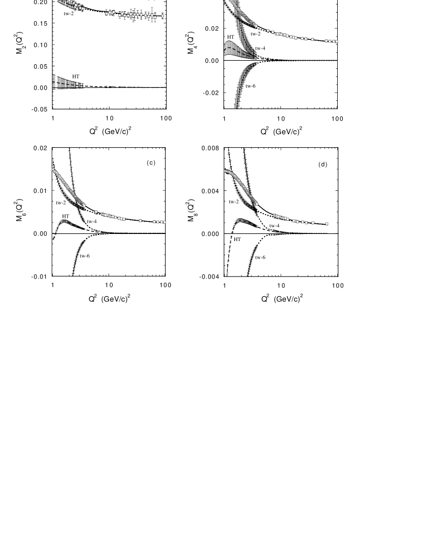
Figure 11: Results of the twist analysis. The open squares represent the Nachtman moments obtained in this analysis. The solid line is the fit to the moments using Eq. 37 with the parameters listed in Table 3. The twist-2, twist-4, twist-6 and higher twist (HT) contributions to the fit are indicated. The twist-2 contribution was calculated using Eq. 39.

Figure 12: Ratio of the total higher-twist (see Eq. 38) to the leading twist given in Eq. 39. Dotted line - $M_{2}$; Dash-dotted line - $M_{4}$; dashed line - $M_{6}$; continuous line - $M_{8}$.

V Conclusions

We extracted the $F_{2}$ structure function in a continuous two-dimensional range of $Q^{2}$ and $x$ from the inclusive cross section measured with the CLAS detector. Using these data, together with the previously available world data set, we evaluated the Nachtmann moments $M_{2}(Q^{2},x)$, $M_{4}(Q^{2},x)$, $M_{6}(Q^{2},x)$ and $M_{8}(Q^{2},x)$ in the $Q^{2}$ range $0.05-100$ (GeV/c)². The present data set covers a large interval in $x$ thus reducing the uncertainties in the integration procedure. The Nachtmann moments obtained in this work have been analyzed in terms of a twist expansion in order to simultaneously extract both the leading and the higher twists. The former has not been treated at fixed order in perturbation theory, but higher-order corrections of pQCD were taken into account by means of soft gluon resummation techniques. Higher twists have been treated phenomenologically by introducing effective anomalous dimensions. The range of the analysis was quite large, ranging from $1$ to $100$ (GeV/c)². The leading twist is determined with a few percent uncertainty, while the precision of the higher twists increases with $n$ reaching an overall $10$% for $n=6$ and $8$, thanks to the remarkable quality of the experimental moments.

The main results of our twist analysis can be summarized as follows:   i) the contribution of the leading twist calculated in the frame of pQCD at NLO remains dominant down to $2Q^{2}/n\sim 1$ (GeV/c)², where $n$ is the moment order. This leads to the conclusion that a pQCD-based description of the proton structure is relevant also at low $Q^{2}$, with significant but not crucial corrections;   ii) the total contribution of the multi-parton correlation effects is not negligible for $Q^{2}<5$ (GeV/c)² and large $x$ corresponding to the resonance region. This can be seen by comparing the higher twist contribution to $M_{8}$, which is more heavily weighted in $x$, to $M_{2}$;   iii) different higher twist terms tend to compensate each other in such a way that their sum is small even in a $Q^{2}$ region where their absolute contributions exceed the leading twist. This cancellation is responsible for the duality phenomena and leads to the prevailing DIS-inspired picture of photon-proton collisions at low $Q^{2}$.

Therefore, we demonstrated that a precise determination of higher twists is feasible with the high quality of the new CLAS data. The main limitation of the present analysis is the use of a phenomenological ansatz for the higher twists. In this respect it is necessary to have better theoretical knowledge of the renormalization group behaviour of the relevant higher-twist operators. This would directly test QCD in its non-perturbative regime through the comparison of predictions obtained from lattice simulations with these data.

Appendix A Fit of the ratio $R\equiv\sigma_{L}/\sigma_{T}$

The function $R(x,Q^{2})=\sigma_{L}/\sigma_{T}$ was described as:

$$R(x,Q^{2})=$$

$$\left\{\begin{array}[]{ll}\frac{(1-x)^{3}}{(1-x_{th})^{3}}\bigl{[}\frac{0.041\xi_{th}}{\zeta}+\frac{0.592}{Q^{2}}-\frac{0.331}{(0.09+Q^{4})}\bigr{]}&W<2.5~{},\\ \\ \frac{0.041\xi}{\zeta}+\frac{0.592}{Q^{2}}-\frac{0.331}{(0.09+Q^{4})}&W>2.5{}\end{array}\right.$$ (45)

This parametrization of $R(x,Q^{2})$ consists of two different parts: the fit for the DIS region ($W>2.5$ GeV) Whitlow_R ; bar and the function, adjusted to scarce data at small $Q^{2}$ BurkertPP ; Ratio1 ; Ratio2 , in the resonance region ($W<2.5$ GeV). The systematic error on this parametrization was estimated according to Ref. Ricco1 as follows:

$$\delta_{R}=\left\{\begin{array}[]{ll}0.08&W<2.5~{},\\ \\ \frac{0.006\xi}{\zeta}+\frac{0.01}{Q^{2}}-\frac{0.01}{(0.09+Q^{4})}&W>2.5{}\end{array}\right.$$ (46)

where

$$\zeta=\log{\frac{Q^{2}}{0.04}}$$ (47)

$$\xi=1+12\frac{Q^{2}}{1+Q^{2}}\frac{0.015625}{0.015625+x^{2}}$$

$$\xi_{th}=\xi(W=2.5)$$

$$x_{th}=x(W=2.5)$$

All dimensional variables are given in GeV.

References

- (2) BloGil E. Bloom and F. Gilman, Phys. Rev. Lett. 25, 1140 (1970); Phys. Rev. D4, 2901 (1971).
- (4) C.S. Armstrong et al., Phys. Rev. D63, 094008 (2001).
- (5) A. De Rujula, H. Georgi and H. Politzer, Ann. Phys. 103, 315 (1977).
- (6) J.M. Cornwall and R.E. Norton, Phys. Rev. 177, 2584 (1969).
- (7) G. Ricco et al., Phys. Rev. C57, 356 (1998).
- (8) I. Niculescu et al., Phys. Rev. D60, 094001 (1999).
- (9) I. Niculescu et al., Phys. Rev. Lett. 85, 1186 (2000); Phys. Rev. Lett. 85, 1182 (2000).
- (10) P.E. Bosted et al., Phys. Rev. C51, 409 (1995).
- (11) M.K. Jones et al., Phys. Rev. Lett. 84, 1398 (2000).
- (12) M. Osipenko et al., CLAS-NOTE-2003-001, (2003).
- (13) O. Nachtmann, Nucl. Phys. B63, 237 (1973).
- (14) R.G. Roberts, The structure of the proton, Cambridge University Press (1990).
- (15) M. Beneke, CERN-TH/98-233; M. Maul et al., Phys. Lett. B401, 100 (1997); M. Dasgupta and B.R. Webber, Phys. Lett. B382, 273 (1996); E. Stein et al., Phys. Lett. B376, 177 (1996).
- (16) G. Ricco et al., Nucl. Phys. B555, 306 (1999).
- (17) S. Catani et al., CERN-TH/96-86; M. Cacciari and S. Catani, CERN-TH/2001-174.
- (18) S. Simula, Phys. Lett. B493, 325 (2000).
- (19) M. D. Mestayer et al., Nucl. Instr. and Meth. A449, 81 (2000).
- (20) E. S. Smith et al., Nucl. Instr. and Meth. A432, 265 (1999).
- (21) G. Adams et al., Nucl. Instr. and Meth. A465, 414 (2001).
- (22) M. Amarian et al., Nucl. Instr. and Meth. A460, 460 (2001).
- (23) A. Bodek et al., Phys. Rev. D20, 1471 (1979).
- (24) S. Stein et al., Phys. Rev. D12, 1884 (1975).
- (25) P. Bosted, private communication.
- (26) D. Wiser, Ph.D. thesis, University of Wisconsin (1977).
- (27) L.W. Mo and Y.S. Tsai, Rev. Mod. Phys. 41, 205 (1969); Yung-Su and Tsai, Phys. Rev. 122, 1898 (1961).
- (28) http://improv.unh.edu/Maurik/gsim_info.shtml.
- (29) I. Akushevich et al., Acta Phys. Polon. B28, 563 (1997).
- (30) S.I. Bilenkaya et al., JETP Lett. 19, 317 (1974).
- (31) F.W. Brasse et al., Nucl. Phys. B110, 413 (1976).
- (32) A.C. Benvenuti et al.,Phys. Lett. B223, 485 (1989).
- (33) M.R. Adams et al., Phys. Rev. D54, 3006 (1996).
- (34) M. Arneodo et al., Nucl. Phys. B483, 3 (1997).
- (35) I. Abt et al., Nucl. Phys. B407, 515 (1993).
- (36) T. Ahmed et al., Nucl. Phys. B439, 471 (1995).
- (37) T. Ahmed et al., Nucl. Phys. B470, 3 (1996).
- (38) C. Adloff et al., Nucl. Phys. B497, 3 (1997).
- (39) C. Adloff et al., DESY-99-107, (1999).
- (40) M. Derrick et al., Phys. Lett. B316, 412 (1993).
- (41) M. Derrick et al., Z. Phys. C65, 379 (1995).
- (42) M. Derrick et al., Z. Phys. C69, 607 (1995).
- (43) M. Derrick et al., Z. Phys. C72, 399 (1996).
- (44) J. Brietweg et al., Phys. Lett. B407, 432 (1997).
- (45) J. Brietweg et al., Eur. Phys. J. C7, 609 (1999).
- (46) L.W. Whitlow et al., Phys. Lett. B282, 475 (1992).
- (47) M. Mestayer, SLAC-214, (1978); W.B. Atwood et al., Phys. Lett. B64, 479 (1976); E.M. Riordan et al., SLAC-PUB-1634, (1975); A. Bodek et al., Phys. Rev. Lett. 30, 1087 (1973); J.S. Poucher et al., Phys. Rev. Lett. 32, 118 (1974); G. Miller Phys. Rev. D5, 528 (1972); E.D. Bloom et al., SLAC-PUB-653, (1971); M. Breidendach, MIT-2098-635, (1970).
- (48) http://wwwinfo.cern.ch/asd/cernlib/overview.html.
- (49) J.J. Aubert et al., Nucl. Phys. B259, 189 (1985).
- (50) A. Milsztajn et al., Z. Phys. C49, 527 (1991).
- (51) D. Allasia et al., Z. Phys. C28, 321 (1991).
- (52) F. W. Brasse et al., DESY-67-34 (1967); W. Albrecht et al., Phys. Lett. B28, 225 (1968); W. Albrecht et al., Nucl. Phys. B13, 1 (1969).
- (53) B. Adeva et al., Phys. Rev. D58, 112001 (1998).
- (54) S. Forte et al., hep-ph/0204232, (2002).
- (55) X. Ji and P. Unrau, Phys. Rev. D52, 72 (1995); U.K. Yang and A. Bodek, Phys. Rev. Lett. 82, 2467 (1999).
- (56) Particle Data Group, D.E. Groom et al., Eur. Phys. Jour. C15, 1 (2000).
- (57) L.W. Whitlow et al., Phys. Lett. B250, 193 (1990).
- (58) J. Bartelski et al., hep-ph/9804415, (1998).
- (59) V. Burkert, CEBAF-PR-93-035, (1993).
- (60) J. Drees et al., Z. Phys. C7, 183 (1981).
- (61) L.M. Stuart et al., Phys. Rev. D58, 032003 (1998).