Spectral quark model and low-energy hadron phenomenology

Abstract

We propose a spectral quark model which can be applied to low energy hadronic physics. The approach is based on a generalization of the Lehmann representation of the quark propagator. We work at the one-quark-loop level. Electromagnetic and chiral invariance are ensured with help of the gauge technique which provides particular solutions to the Ward-Takahashi identities. General conditions on the quark spectral function follow from natural physical requirements. In particular, the function is normalized, its all positive moments must vanish, while the physical observables depend on negative moments and the so-called log-moments. As a consequence, the model is made finite, dispersion relations hold, chiral anomalies are preserved, and the twist expansion is free from logarithmic scaling violations, as requested of a low-energy model. We study a variety of processes and show that the framework is very simple and practical. Finally, incorporating the idea of vector-meson dominance, we present an explicit construction of the quark spectral function which satisfies all the requirements. The corresponding momentum representation of the resulting quark propagator exhibits only cuts on the physical axis, with no poles present anywhere in the complex momentum space. The momentum-dependent quark mass compares very well to recent lattice calculations. A large number of predictions and relations, valid at the low-energy scale of the model, can be deduced from our approach for such quantities as the pion light-cone wave function, non-local quark condensate, pion transition form factor, pion valence parton distribution function, etc. These quantities, obtained at a low-energy scale of the model, have correct properties, as requested by symmetries and anomalies. They also have pure twist expansion, free of logarithmic corrections, as requested by the QCD factorization property.

I Introduction

The term chiral quark model has become a generic name for any relativistic field theory aiming at the description of the non-perturbative features of QCD. Numerous approaches (for reviews see, e.g., Vogl and Weise (1991); Klevansky (1992); Volkov (1993); Hatsuda and Kunihiro (1994); Christov et al. (1996); Alkofer et al. (1996); Ripka (1997); Ruiz Arriola (2002), and references therein) share a number of common features. Firstly, they incorporate dynamical quarks as the only explicit degrees of freedom. Secondly, they provide particular solutions to the chiral and electromagnetic Ward-Takahashi identities. Although there is no doubt that chiral quark models provide a reasonably accurate quantitative description of hadronic properties, there is a lack of systematics in the construction of any particular dynamical model. A source of ambiguity is the fact that chiral quark models are, supposedly, an approximation to the low-energy non-perturbative QCD dynamics. In this regard, an essential ingredient is the introduction of a practical suppression of high-energy degrees of freedom, necessary in order to separate the low-energy regime, where the model is supposed to work, and the high-energy regime, where the genuine QCD dynamics, in terms of explicit quarks and gluons, should set in. This defines a certain scale, or cut-off, which acquires a physical meaning and which should be kept throughout the calculation. The precise way how this high-energy cut-off should be introduced is not at all clear, although some constraints can be imposed on the basis of the relativistic and gauge invariance. For a discussions of various popular approaches and associated problems see, e.g., Ruiz Arriola (2002).

In this work we introduce a novel approach, the spectral regularization of the chiral quark model, based on the formal introduction of the Lehmann representation Itzykson and Zuber (1980) for the quark propagator,

$$S({p})=\int_{C}d\omega{\rho(\omega)\over\hbox to0.0pt{\hbox to5.03125pt{\hfil/\hfil}\hss}p-\omega},$$ (1)

where $\rho(\omega)$ is the spectral function and $C$ denotes a contour in the complex $\omega$ plane chosen in a suitable way. As will become clear in Sect. III, the spectral regularization allows to explicitly solve the chiral and electromagnetic Ward-Takahashi identities in a rather simple manner, through the use of the so-called gauge technique Delbourgo and West (1977); Delbourgo (1979). The method has already been sketched in a previous work by one of us Arriola (2001). Of course, any solution of the Ward-Takahashi identities cannot be complete due to the existence of transverse terms, which necessarily appear in the underlying theory, and which can only be uniquely determined in QCD. In fact, any possible realization of a chiral quark model, if properly regularized, represents in a sense a particular solution to the Ward-Takahashi identities. This point is not fully appreciated. In Sect. III we will provide a minimal set of solutions to the Ward-Takahashi identities and study their consequences.

Throughout the paper the model is considered at the one-quark-loop level and in the chiral limit of the vanishing current quark masses. Therefore our present predictions are made at the leading-$N_{c}$ level and in the chiral limit.

The proper normalization and the conditions of finiteness of hadronic observables are achieved by requesting what we call the spectral conditions for the moments of the quark spectral function, $\rho(\omega)$, namely

$$\rho_{0} \equiv\int d\omega\rho(w)=1,$$ (2)

$$\rho_{n} \equiv\int d\omega\omega^{n}\rho(\omega)=0,\;\;\;{\rm for}\;n=1,2,3,...$$ (3)

It will be shown that the physical observables are proportional to the inverse moments,

$$\rho_{-k} \equiv\int d\omega\omega^{-k}\rho(\omega),\;\;\;{\rm for}\;k=1,2,3,...$$ (4)

as well as to the “log moments”,

$$\rho^{\prime}_{n}\equiv\int d\omega\log(\omega^{2}/\mu^{2})\omega^{n}\rho(\omega)$$

$$=\int d\omega\log(\omega^{2})\omega^{n}\rho(\omega),\;\;\;{\rm for}\;n=2,3,4,...$$ (5)

Note that the conditions (3) remove the dependence on the scale $\mu$ in (5), thus we can drop it. No standard requirement of positivity for the spectral strength, $\rho(\omega)$, is made (see Sect. II.4).

In the present work we do not intend to determine the quark spectral function from “first principles”, but rather look for general consequences and implicit relations which follow from the approach.

The model with the spectral regularization (1,2,3), supplied with couplings obtained via the gauge technique, possesses simultaneously the following features:

1. Gives finite values for hadronic observables, which can be used to fix the inverse moments, (4), and the log moments, (5).

2. Satisfies by construction the electromagnetic and chiral Ward-Takahashi identities, thus reproducing all the necessary symmetry requirements.

3. Satisfies the anomaly conditions.

4. Complies to the QCD factorization property, in the sense that the expansion of a correlator in a large-momentum $Q$ is a pure twist-expansion involving only the inverse powers of $Q^{2}$, without the $\log Q^{2}$ corrections. Thus, the model can be used to compute the soft matrix elements needed to describe the deep inelastic inclusive and exclusive processes and to analyze the pion structure function, pion distribution amplitude, etc.

The fact that all above features can be satisfied simultaneously in a chiral quark model is far from trivial Ruiz Arriola (2002).

One of the advantages of our regularization is that all calculations can be directly undertaken in the Minkowski space, although nothing prevents us from working in the Euclidean space. When dealing with bound-state problems, the continuum Euclidean formulation encounters practical difficulties in momentum space since going to the bound state pole requires a continuation to the Minkowski region, and hence a continuation of the quark propagator to the complex plane is required. This is a problem since much of our phenomenological insight is based on the behavior of the quark propagator in the Euclidean region. In our approach the analytic continuation from the Euclidean to the Minkowski space can be done in a straightforward manner because the generalized Lehmann representation (1) implies a definite analytic structure.

In the language of the practitioners of chiral quark models such as the Nambu–Jona-Lasinio model, the regularization introduced by the gauge technique is very special because not only it makes the theory finite, but also corresponds to taking the infinite cut-off limit in those observables which do not depend on the constituent quark mass. This includes the proper fulfillment of the anomalies. As we will see below, this is a very rewarding aspect of the present investigation, which avoids the artificial separation between the real and imaginary parts in the Euclidean action, or, equivalently, the normal and abnormal parity processes in the Minkowski space. At the same time, the study of several processes in the high-energy limit turns out to be compatible with factorization of amplitudes into hard and soft pieces in the twist expansion precisely because of the regularization and the set of conditions (2,3) imposed upon the spectral function $\rho(\omega)$. Although such a behavior is expected in perturbative QCD, it is very difficult to comply to it in traditional chiral quark models. This point has been recently discussed by one of us in Ref. Ruiz Arriola (2002), where it is pointed out that for the process $\gamma^{*}\to\pi^{0}\gamma$, which involves the transition form factor $F_{\gamma^{*}\pi^{0}\gamma}(Q^{2})$, there is a conflict between the chiral anomaly normalization condition for $F_{\gamma^{*}\pi^{0}\gamma}(0)=1/(4\pi f_{\pi})$, and the expected QCD factorization at large momenta, $Q^{2}F_{\gamma^{*}\pi^{0}\gamma}(Q^{2})\to 2f_{\pi}$. The conflict persists in any standard approach; to fulfill the anomaly the absence of a regulator is required, but to achieve factorization an explicit regularization must be considered. Our model is free of such contradictions, and both conditions turn out to be satisfied simultaneously. Actually, as we show in Sects. VIII and X, for the pion the leading twist contribution to the parton distribution function (PDF), $V_{\pi}(x)$, and the parton distribution amplitude (PDA), $\varphi_{\pi}(x)$ the following remarkable relation holds at the model’s scale $Q_{0}$:

$$\varphi_{\pi}(x,Q_{0})=\frac{1}{2}V_{\pi}(x,Q_{0})=1.$$ (6)

We stress that the interpretation of results of low-energy models in the context of the high-energy processes necessarily involves QCD evolution to account for logarithmic perturbative radiative corrections. The soft matrix elements computed in the model are obtained at the working energy scale of the model, $Q_{0}$, typically quite low, and have to be evolved to the scales realized experimentally with help of the QCD evolution. Only then the comparison to data can be made Jaffe and Ross (1980); Jaffe (1986). In that sense, chiral quark models provide the initial conditions for the QCD evolution. The phenomenological success of Eq. (6) after evolution has been described elsewhere Davidson and Arriola (1995, 2002); Arriola and Broniowski (2002); Ruiz Arriola (2002).

In Sect. XII we provide a model for the moments (4) of the spectral function based on the vector-meson dominance (VMD) in the pion electromagnetic form factor. Actually, only the even and negative moments are determined by such a method. Remarkably, the positive moments obtained by analytic continuation automatically fulfill the spectral conditions, Eq. (2,3), and the log-moments (5) can also be determined. Interestingly, the inverse-moment problem for the VMD-inspired model can be solved, yielding a simple function with a certain cut-structure in the complex $\omega$-plane. As a result, the model becomes fully explicit and some further results can be obtained. Using the insight provided by the VMD model we work out in Sect. XIII the quark propagator, which possesses a certain cut structure but has no poles in the whole complex plane. The quark mass function agrees remarkably well with recent lattice data Bowman et al. (2002a, b). We illustrate the power of the method in Sect. XIV by presenting some further predictions based on the VMD model, namely, the pion transition form factor, the pion light cone wave function, the non-local quark condensate, and the unintegrated parton distribution function of the pion.

II Quark propagator

II.1 Generalized spectral representation for the quark propagator

Our starting point is the definition of the quark propagator. In the momentum space we have

$$S({p})=-i\int d^{4}xe^{ip\cdot x}\langle 0|T\left\{q(x)\bar{q}(0)\right\}|0\rangle.$$ (7)

We assume the spectral representation (1) for the quark propagator, where $\rho(\omega)$ is the spectral function, and $C$ is a contour in the complex $\omega-$plane chosen in a suitable way. We do not specify explicitly what the contour $C$ is, hence the representation (1) is a generalization of the standard Lehmann representation Itzykson and Zuber (1980). To see the connection, let us consider the special example of a contour $C$ running from $-\infty$ under the real negative axis and crossing through zero above the real positive axis going to $+\infty$, yielding the form proposed in Ref. Delbourgo and West (1977)

$$S({p})=\int_{-\infty}^{\infty}d\omega{\rho(\omega)\over\hbox to0.0pt{\hbox to5.03125pt{\hfil/\hfil}\hss}p-\omega+{i}\epsilon(\omega)},$$ (8)

where $\epsilon(\omega)=0^{+}{\rm sgn}(\omega)$. Squaring the denominator in Eq.(8) yields a more customary form of the Lehmann representation Itzykson and Zuber (1980),

$$S(p) = \int_{0}^{\infty}d\omega\frac{\hbox to0.0pt{\hbox to5.03125pt{\hfil/\hfil}\hss}p\rho_{V}(\omega)+\omega\rho_{S}(\omega)}{p^{2}-\omega^{2}+{i}0^{+}},$$ (9)

where the vector and scalar spectral functions

$$\rho_{V}(\omega) = \rho(\omega)+\rho(-\omega),$$

$$\rho_{S}(\omega) = \rho(\omega)-\rho(-\omega),$$ (10)

are defined for $\omega\geq 0$ respectively. Notice that the functions $\rho_{V}(\omega)$ and $\rho_{S}(\omega)$ are independent of each other. Equivalently, the values of $\rho(\omega)$ for positive and negative values of $\omega$ are also independent of each other. The quark propagator in the standard Lehmann representation has an analytic structure of poles and cuts on the real axis of the complex $p^{2}-$plane, where the positivity conditions $\rho_{V}(\omega)\geq 0$ and $\rho_{V}(\omega)\geq\rho_{S}(\omega)$ for $\omega\geq 0$ hold. With Eqs. (10), the positivity conditions are equivalent to saying that $\rho(\omega)\geq 0$ for any $\omega$, positive or negative. They follow from the requirement of a physical Hilbert. We will see in Sect. II.4 that chiral symmetry breaking, together with the finiteness of hadronic observables, implies that in our case a real $\rho(\omega)$ cannot be positive definite, which is a simple consequence of the conditions (2,3) if the contour is taken to be the standard one. Actually, the particular realization proposed below in Sect. XII based on the vector-meson dominance of the electromagnetic pion form factor shows that one needs in fact a non-trivial contour to avoid end-point singularities. We refrain from speculating on the possible connection of this fact to an indication of quark confinement, nevertheless it is certainly true that a non-positive spectral function cannot be understood in terms of physical particles on the mass shell. On the other hand, a non-trivial quark propagator must depend non-trivially on momentum if it is defined in the whole complex plane. As will become clear in Sect. XIII, a VMD-based model produces a complex spectral function $\rho(\omega)$ on a complex contour $C$, which results in a quark propagator with cuts only.

In a model without confinement the spectral representation of a propagator is a well defined concept. In a gauge theory, like QED, the spectral representation depends on the particular gauge, because the two-point function does. In a theory with confinement not much is known about the analytic properties of the quark propagator, except for the fact that poles at real positive values of $p^{2}$ with positive residues are certainly excluded. In QCD such a representation certainly exists in perturbation theory where confinement is not manifest. The study of $\rho(\omega)$ within QCD yields at LO, for $m\to 0$, the following expression Haeri (1988):

$$\rho(\omega)=\delta(\omega-m)+{\rm sign}(\omega)\frac{\alpha C_{F}}{4\pi}\frac{1-\xi}{\omega}\theta(\omega^{2}-m^{2}),$$ (11)

where $\xi$ is the gauge parameter. However, if the general representation is valid, its detailed properties may be quite different in the non-perturbative regime.

As will become clear below, the real strength of the ansatz (1) relies in the fact that having assumed certain properties of $\rho(w)$ reduces the calculations of physical observables to nothing more than the standard one-loop analysis. In addition, it allows for going from the Euclidean to the Minkowski space, back and forth. Thus, our assumption is essentially that of analyticity of the quark propagator $S(p)$, and the possibility to analytically continue it in the whole complex plane. This looks, in principle, very different from the approach invoked in non-local models, where only the Euclidean region is used to justify the propagator. Nevertheless, calculation of physical observables require in practice an extrapolation into the complex $p^{2}$-plane, which by itself can only be justified through analytic continuation. The previous argument does not justify Eq. (1), but it shows that we are not making any additional assumptions as compared to those implied in non-local models.

Although in perturbation theory the integration contour may be kept on the real axis, there are cases where singularities may pinch the integration path. This circumstance becomes a problem, since either analyticity or relativistic invariance may be spoiled. In this regard a number of prescriptions have been devised in order to avoid such a situation Lee and Wick (1969); Cutkosky et al. (1969); Boulware and Gross (1984). Thus, in general, we will assume that the integration path is an arbitrary contour chosen in a convenient way. This contour integration requires effectively considering complex masses. Genuine non-local models formulated in the Minkowski space also require a specification of the integration contour in momentum space in order to keep relativistic invariance Praszałowicz and Rostworowski (2001). An example of a definite prescription of the choice of such a contour is given in Sect. XII.

The quark propagator (1) may be parameterized in the standard form,

$$S(p)=A(p)\hbox to0.0pt{\hbox to5.03125pt{\hfil/\hfil}\hss}p+B(p)=Z(p)\frac{\hbox to0.0pt{\hbox to5.03125pt{\hfil/\hfil}\hss}p+M(p)}{p^{2}-M^{2}(p)},$$ (12)

with

$$A(p) = \int d\omega\frac{\rho(\omega)}{p^{2}-\omega^{2}},$$

$$B(p) = \int d\omega\frac{\rho(\omega)\omega}{p^{2}-\omega^{2}},$$ (13)

and the mass and wave function renormalization functions given by

$$M(p) = \frac{B(p)}{A(p)},$$ (14)

$$Z(p) = (p^{2}-M^{2}(p))A(p),$$ (15)

respectively. Let us note that if we had $\rho(\omega)=\rho(-\omega)$, then the quark mass would vanish, $M(p^{2})=0$, and spontaneous breaking of the chiral symmetry would then be precluded. Thus, in general, we expect $\rho(\omega)$ not to be an even function. In the following sections we will compute one-by-one the physical observables and accumulate conditions that have to be satisfied by the moments of the spectral function $\rho(\omega)$.

II.2 Quark condensate

With help of the representation (1) the quark condensate (for a single flavor) may be straightforwardly computed, yielding

$$\langle\bar{q}q\rangle = -iN_{c}\int d\omega\rho(\omega)\int{d^{4}p\over(2\pi)^{4}}{\rm Tr}{1\over\hbox to0.0pt{\hbox to5.03125pt{\hfil/\hfil}\hss}p-\omega}$$ (16)

$$= -4iN_{c}\int d\omega\rho(\omega)\int{d^{4}p\over(2\pi)^{4}}{\omega\over p^{2}-\omega^{2}},$$

where the trace is over the Dirac space, and $N_{c}=3$ is the number of colors. The integral over the momentum $p$ is quadratically divergent. This requires the use of an auxiliary regularization method, removed at the end of the calculation. With three-dimensional cut-off, $\Lambda$, one gets for large $\Lambda$

$$\langle\bar{q}q\rangle = -{N_{c}\over 4\pi^{2}}\int d\omega\omega\rho(\omega)\left[2\Lambda^{2}+\omega^{2}\log\left(\frac{\omega^{2}}{4\Lambda^{2}}\right)+\omega^{2}\right].$$

The finiteness of the result at $\Lambda\to\infty$ requires the conditions

$$\rho_{1}=0,\;\;\;\rho_{3}=0,$$ (18)

and thus

$$\langle\bar{q}q\rangle=-{N_{c}\over 4\pi^{2}}\int d\omega\log(\omega^{2})\omega^{3}\rho(\omega)=-{N_{c}\over 4\pi^{2}}\rho^{\prime}_{3}.$$ (19)

Exactly the same conclusions are reached if the four-momentum auxiliary regularization is introduced. Note that the $\rho_{3}=0$ spectral condition allowed for rewriting $\log(\omega^{2}/\Lambda^{2})$ as $\log(\omega^{2})$, hence no scale dependence (no “dimensional transmutation”) is present in the final expression. The dimensional regularization in $4+\varepsilon$ dimensions, gives

$$\langle\overline{q}q\rangle = \frac{N_{c}}{4\pi^{2}}\int d\omega\rho(\omega)\omega^{3}\left[-\log\left(\omega^{2}/\mu^{2}\right)-\frac{1}{\varepsilon}+1\right].$$

However, the dimensional regularization “hides” some conditions, for instance here it leads only to the $\rho_{3}=0$ condition, and does not require the $\rho_{1}=0$ condition. This is due to the fact that in the dimensional regularization the power divergences have a fixed ratio.

Finally, we remark that in the perturbative phase with no spontaneous symmetry breaking, where $\rho(\omega)=\rho(-\omega)=\delta(\omega)$, we have $\langle\bar{q}q\rangle=0$. With the accepted value of

$$\langle\bar{q}q\rangle=\langle\bar{u}u\rangle=\langle\bar{d}d\rangle\simeq-(243~{}{\rm MeV})^{3}$$ (20)

(at the typical hadronic scale of $0.5-1$ GeV) Ioffe (2002) we can infer the value of the third log-moment, $\rho^{\prime}_{3}$. The sign of the quark condensate shows that

$$\rho^{\prime}_{3}>0.$$ (21)

II.3 Non-local quark condensate

In various QCD studies (see e.g. Refs. Mikhailov and Radyushkin (1989, 1992); Bakulev and Mikhailov (2002); Dorokhov and Broniowski (2002) and references therein) the non-local quark condensate,

$$Q(x)\equiv\frac{\langle q(0)q(x)\rangle}{\langle q(0)q(0)\rangle},$$ (22)

plays an important role. In our approach

$$\langle\bar{q}(0)q(x)\rangle = -4iN_{c}\int d\omega\rho(\omega)\int{d^{4}p\over(2\pi)^{4}}{\omega\over p^{2}-\omega^{2}}e^{ip\cdot x},$$

and, consequently, after performing the Fourier-Bessel transform,

$$Q(x)=\frac{1}{\rho^{\prime}_{3}}\int d\omega\rho(\omega)4\omega^{3}\frac{K_{1}(\sqrt{-\omega^{2}x^{2}})}{\sqrt{-\omega^{2}x^{2}}},$$ (24)

where $x$ denotes the Minkowski coordinate. A related quantity is the average vacuum virtuality of the quarks, $\lambda_{q}$, defined through

$$\lambda_{q}^{2}\equiv\frac{\langle\bar{q}(\partial^{2})q\rangle}{\langle\bar{q}q\rangle}.$$ (25)

With our spectral regularization method we find that

$$\frac{\langle\bar{q}(\partial^{2})^{n}q\rangle}{\langle\bar{q}q\rangle} \equiv \frac{\int d\omega\rho(\omega)\int{d^{4}p}{(-p^{2})^{n}\omega/(p^{2}-\omega^{2})}}{\int d\omega\rho(\omega)\int{d^{4}p}{\omega/(p^{2}-\omega^{2})}}$$ (26)

$$= (-)^{n}\frac{\rho^{\prime}_{2n+3}}{\rho^{\prime}_{3}},$$

in particular

$$\lambda_{q}^{2}=-\frac{\rho^{\prime}_{5}}{\rho^{\prime}_{3}},$$ (27)

while the QCD sum rules estimates suggest the value $\lambda_{q}^{2}\simeq 0.5\pm 0.1~{}{\rm GeV}^{2}$ Belyaev and Ioffe (1982). The positivity of $\lambda_{q}^{2}$ and $\rho^{\prime}_{3}$ (see Sect. II.2) enforces

$$\rho^{\prime}_{5}<0.$$ (28)

II.4 Vacuum energy density

Continuing the quest for the conditions on the spectral function $\rho(\omega)$ we now study the vacuum energy density. The energy-momentum tensor for a purely quark model is defined as

$$\theta^{\mu\nu}(x)=\bar{q}(x)\frac{i}{2}\left\{\gamma^{\mu}\partial^{\nu}+\gamma^{\nu}\partial^{\mu}\right\}q(x)-g^{\mu\nu}{\cal L}(x).$$

(29)

At the one-quark-loop level

$$\langle\theta^{\mu\nu}\rangle=-iN_{c}N_{f}\int d\omega\rho(\omega)\int{d^{4}p\over(2\pi)^{4}}\times$$

$${\rm Tr}{1\over\hbox to0.0pt{\hbox to5.03125pt{\hfil/\hfil}\hss}p-\omega}\left[\frac{1}{2}\left(\gamma^{\mu}p^{\nu}+\gamma^{\nu}p^{\mu}\right)-g^{\mu\nu}(\hbox to0.0pt{\hbox to5.03125pt{\hfil/\hfil}\hss}p-\omega)\right]$$

$$=-4iN_{c}N_{f}\int d\omega\rho(\omega)\int{d^{4}p\over(2\pi)^{4}}{p^{\mu}p^{\nu}-g^{\mu\nu}(p^{2}-\omega^{2})\over p^{2}-\omega^{2}}$$

$$=Bg^{\mu\nu}+\langle\theta^{\mu\nu}\rangle_{0},$$ (30)

where $N_{f}$ is the number of flavors and $\langle\theta^{\mu\nu}\rangle_{0}$ is the energy-momentum tensor for the free theory, i.e. evaluated with $\rho(\omega)=\delta(\omega)$. The quantity $B$ is the vacuum energy density given by

$$B=-iN_{c}N_{f}\int d\omega\rho(\omega)\int{d^{4}p\over(2\pi)^{4}}{\omega^{2}\over p^{2}-\omega^{2}},$$ (31)

where in the subtraction of the free part we have used the spectral condition (2). The integral over $p$ is quadratically divergent, but there is an additional power of $\omega$ as compared to the case of the quark condensate. Hence, the conditions that have to be fulfilled for $B$ to be finite are $\rho_{2}=0$ and $\rho_{4}=0$. Then

$$B=-{N_{c}N_{f}\over 16\pi^{2}}\rho^{\prime}_{4}=-{3N_{c}\over 16\pi^{2}}\rho^{\prime}_{4}$$ (32)

for three flavors, $N_{f}=3$, used from now on.

Interestingly, the even conditions (here quadratic and quartic) imply that $\rho(\omega)$ cannot be positive definite; otherwise the even moments could not vanish.

An alternative expression for $B$ can be obtained from integrating by parts in the variable $p$ and using the conditions $\rho_{2}=\rho_{4}=0$,

$$B=2iN_{c}N_{f}\int d\omega\rho(\omega)\int{d^{4}p\over(2\pi)^{4}}\log(p^{2}-\omega^{2}),$$ (33)

which reminds us of the vacuum energy density calculated in the effective action formalism. Another interesting version of $B$ is obtained by integrating Eq. (31) with respect to the variable $p_{0}$ first, when we get

$$B=-2N_{c}N_{f}\int d\omega\rho(\omega)\int\frac{d^{3}k}{(2\pi)^{3}}\sqrt{k^{2}+\omega^{2}}.$$ (34)

The interpretation of this equation is obvious: $B$ is a weighted integral of negative energy quarks with constituent mass $\omega$. Upon imposing the $\rho_{2}=0$ and $\rho_{4}=0$ conditions the integration of the three momentum integral yields Eq. (32).

In the case of spontaneous chiral symmetry breaking one expects, $\langle\theta_{00}\rangle<\langle\theta_{00}\rangle_{0}$, or $B<0$. According to the most recent QCD sum rules analysis for charmonium  Ioffe and Zyablyuk (2002); Ioffe (2002), one has, for three flavors,

$$B=-\frac{9}{32}\langle\frac{\alpha}{\pi}G^{2}\rangle=-(224^{+35}_{-70}{\rm MeV})^{4}.$$ (35)

Note the large uncertainty in this result. The negative sign of $B$ enforces

$$\rho^{\prime}_{4}>0.$$ (36)

II.5 Low- and high-momentum behavior

At low momenta we may formally expand the quark propagator (8) to obtain

$$S(p)=-\sum_{k=0}^{\infty}\int d\omega\frac{\rho(\omega)}{\omega}\left(\frac{\hbox to0.0pt{\hbox to5.03125pt{\hfil/\hfil}\hss}p}{\omega}\right)^{k}=-\sum_{k=0}^{\infty}\rho_{-k-1}\hbox to0.0pt{\hbox to5.03125pt{\hfil/\hfil}\hss}p^{k}.$$ (37)

Hence the low-momentum expansion involves the inverse moments (4). In particular, for $M$ and $Z$ of Eqs. (14,15) we find

$$M(0) = \frac{\rho_{-1}}{\rho_{-2}},$$

$$\left.\frac{dM(p^{2})}{dp^{2}}\right|_{p^{2}=0} = \frac{\rho_{-3}}{\rho_{-2}}-\frac{\rho_{-1}\rho_{-4}}{\rho_{-2}^{2}},$$

$$Z(0) = \frac{\rho_{-1}^{2}}{\rho_{-2}}.$$ (38)

A knowledge of these quantities, for instance from lattice calculations, would help to determine the inverse moments (4) and constrain the spectral function. According to Eqs. (38), the positivity of $Z(0)$ leads to $\rho_{-2}>0$, while combined with the positivity of $M(0)$ gives $\rho_{-1}>0$.

In the limit of large momentum, $p\to\infty$, we formally have

$$S(p) \sim \frac{1}{\hbox to0.0pt{\hbox to5.03125pt{\hfil/\hfil}\hss}p}\int d\omega\rho(w)+\frac{1}{p^{2}}\int d\omega\omega\rho(\omega)$$

$$+ \frac{1}{\hbox to0.0pt{\hbox to5.03125pt{\hfil/\hfil}\hss}p^{3}}\int d\omega\omega^{2}\rho(\omega)+...$$

Normalization of the quark propagator in the asymptotic region to $1/\hbox to0.0pt{\hbox to5.03125pt{\hfil/\hfil}\hss}p$ leads to the condition $\rho_{0}=1$. Furthermore, since $M(p^{2})$ should vanish asymptotically, we conclude that $\rho_{1}=0$.

Note also that if all spectral conditions (2,3) are assumed then the asymptotic large momentum expansion would yield a trivial free massless quark propagator. Thus, the high-momentum expansion cannot represent the full (and non-trivial) propagator. This indicates some non-meromorphic structure in $p$ at infinity. In Sects. XII and XIII we will present a particular realization of this situation.

III Gauge technique and the vertex functions

Up to now we have accumulated the lowest spectral conditions (2,3), up to $n=4$. Higher conditions will appear in the next sections by requesting the twist expansion of correlation functions. First, however, we need to introduce the coupling of currents to quarks.

In QCD, the vector and axial currents are defined as

$$J_{V}^{\mu,a}(x) = \bar{q}(x)\gamma^{\mu}{\lambda_{a}\over 2}q(x),$$ (40)

$$J_{A}^{\mu,a}(x) = \bar{q}(x)\gamma^{\mu}\gamma_{5}{\lambda_{a}\over 2}q(x).$$ (41)

Although our formulas below are valid for the $SU(N_{f})$ flavor symmetry, in this paper we will be concerned mainly with pion properties. This will be understood by replacing the Gell-Mann matrices, $\lambda_{a}$, by the Pauli matrices, $\tau_{a}$. Conservation of the vector current (CVC) and partial conservation of the axial current (PCAC) implies that

$$\partial_{\mu}J_{V}^{\mu,a}(x) = 0,$$ (42)

$$\partial_{\mu}J_{A}^{\mu,a}(x) = \bar{q}(x)\hat{M}_{0}i\gamma_{5}{\lambda_{a}\over 2}q(x),$$ (43)

with $\hat{M}_{0}={\rm diag}(m_{u},m_{d},m_{s})$ denoting the quark mass matrix. Obviously, any effective theory of QCD must incorporate these constraints. CVC and PCAC imply a set of flavor-gauge and chiral Ward-Takahashi identities among correlation functions involving vector currents, axial currents, and quark field operators, which are based on the local current-field commutation rules Renner (1968),

$$\left[J_{V}^{0,a}(x),q(x^{\prime})\right]_{x_{0}=x^{\prime}_{0}} = -\gamma_{5}{\lambda_{a}\over 2}q(x)\delta(\mathchoice{\mbox{\boldmath$\displaystyle x$}}{\mbox{\boldmath$\textstyle x$}}{\mbox{\boldmath$\scriptstyle x$}}{\mbox{\boldmath$\scriptscriptstyle x$}}-\mathchoice{\mbox{\boldmath$\displaystyle x$}}{\mbox{\boldmath$\textstyle x$}}{\mbox{\boldmath$\scriptstyle x$}}{\mbox{\boldmath$\scriptscriptstyle x$}}^{\prime}),$$

$$\left[J_{A}^{0,a}(x),q(x^{\prime})\right]_{x_{0}=x^{\prime}_{0}} = -\gamma_{5}{\lambda_{a}\over 2}q(x)\delta(\mathchoice{\mbox{\boldmath$\displaystyle x$}}{\mbox{\boldmath$\textstyle x$}}{\mbox{\boldmath$\scriptstyle x$}}{\mbox{\boldmath$\scriptscriptstyle x$}}-\mathchoice{\mbox{\boldmath$\displaystyle x$}}{\mbox{\boldmath$\textstyle x$}}{\mbox{\boldmath$\scriptstyle x$}}{\mbox{\boldmath$\scriptscriptstyle x$}}^{\prime}).$$ (44)

A number of results are then obtained essentially for free. In the low-energy regime pions arise as Goldstone bosons, and the standard current algebra properties hold. In the high-energy regime, parton model features such as scaling and the spin-1/2 nature of hadronic constituents may be recovered. If one restricts to the one-quark-loop approximation, the results also provide a particular solution to the large-$N_{c}$ counting rules at the leading order.

To solve the Ward-Takahashi identities we follow the gauge technique proposed in Ref. Delbourgo and West (1977) (see also Ref. Delbourgo (1979, 1999)) which has the nice feature of linearizing the equations, since they deal with unamputated Green functions. This is in contrast to the more standard approach of writing the Ward-Takahashi identities for amputated Green functions, in which case non-linear equations arise. The gauge technique has been mostly used in the past as a way to obtain solutions to the Schwinger-Dyson equations, both in QED Delbourgo and West (1977); Sauli (2002) and in QCD Haeri (1988). Only recently it has been used to study hadron phenomenology Arriola (2001).

III.1 Vertices with One Current

The vector and axial unamputated vertex functions are defined as

$$\Lambda_{V}^{\mu,a}(p^{\prime},p)=iS(p^{\prime})\Gamma_{V}^{\mu,a}(p^{\prime},p)iS(p)$$

$$= \int d^{4}xd^{4}x^{\prime}\langle 0|T\left\{J_{V}^{\mu,a}(0)q(x^{\prime})\bar{q}(x)\right\}|0\rangle e^{ip^{\prime}\cdot x^{\prime}-ip\cdot x},$$

$$\Lambda_{A}^{\mu,a}(p^{\prime},p)=iS(p^{\prime})\Gamma_{A}^{\mu,a}(p^{\prime},p)iS(p)$$

$$= \int d^{4}xd^{4}x^{\prime}\langle 0|T\left\{J_{A}^{\mu,a}(0)q(x^{\prime})\bar{q}(x)\right\}|0\rangle e^{ip^{\prime}\cdot x^{\prime}-ip\cdot x},$$

respectively. Here the $\Gamma$’s represent the corresponding amputated vertex functions . The Ward-Takahashi identity for the full vector-quark-quark vertex reads

$$(p^{\prime}-p)_{\mu}\Lambda_{V}^{\mu,a}(p^{\prime},p)=S(p^{\prime}){\lambda_{a}\over 2}-{\lambda_{a}\over 2}S(p)\,.$$ (47)

Likewise, for the axial-quark-quark vertex we have

$$(p^{\prime}-p)_{\mu}\Lambda_{A}^{\mu}(p^{\prime},p)=S(p^{\prime}){\lambda_{a}\over 2}\gamma_{5}+\gamma_{5}{\lambda_{a}\over 2}S(p)\,.$$ (48)

The gauge technique, introduced in Ref. Delbourgo and West (1977), consists of writing a solution for the vector unamputated vertex in the form

$$\Lambda_{V}^{\mu,a}(p^{\prime},p)=\int d\omega\rho(\omega){i\over\hbox to0.0pt{\hbox to6.57124pt{\hfil/\hfil}\hss}p^{\prime}-\omega}\gamma^{\mu}{\lambda_{a}\over 2}{i\over\hbox to0.0pt{\hbox to5.03125pt{\hfil/\hfil}\hss}p-\omega}.$$ (49)

The axial-vertex ansatz reads

$$\Lambda_{A}^{\mu}(p^{\prime},p) = \int d\omega\rho(\omega){i\over\hbox to0.0pt{\hbox to6.57124pt{\hfil/\hfil}\hss}p^{\prime}-\omega}\left(\gamma^{\mu}-{2\omega q^{\mu}\over q^{2}}\right)\gamma_{5}{\lambda_{a}\over 2}{i\over\hbox to0.0pt{\hbox to5.03125pt{\hfil/\hfil}\hss}p-\omega}.$$

In this way the Ward-Takahashi identities are linearized. It can be readily verified that these ansätze fulfill the identities (47,48), respectively, up to undetermined transverse pieces. A consequence of the axial Ward-Takahashi identity is the occurrence of a massless pseudoscalar pole identified with the pion, which takes place only if $\rho(\omega)\neq\delta(\omega)$.

The pion wave function, corresponding to the $\pi\to q\bar{q}$ vertex, is defined as

$$\Lambda_{\pi}^{a}(p+q,p)=i\int d^{4}xe^{-ip\cdot x}\langle 0|T\left\{q(0)\bar{q}(x)\right\}|\pi_{a}(q)\rangle.$$

Near the pion pole we get

$$\Lambda_{A}^{\mu,a}(p+q,p)\to-{q^{\mu}\over q^{2}}\Lambda_{\pi}^{a}(p+q,p),$$ (52)

where the pion wave function is given by

$$\Lambda_{\pi}^{a}(p+q,p)=\int d\omega\rho(\omega){i\over\hbox to0.0pt{\hbox to5.03125pt{\hfil/\hfil}\hss}p+\hbox to0.0pt{\hbox to5.00002pt{\hfil$q$\hfil}\hss}/-\omega}\frac{2\omega}{f_{\pi}}\gamma_{5}{\lambda_{a}\over 2}{i\over\hbox to0.0pt{\hbox to5.03125pt{\hfil/\hfil}\hss}p-\omega}.$$

(53)

We recognize in our formulation the Goldberger-Treiman relation for quarks; under the spectral integral over $\omega$ the pseudoscalar coupling of a pion to the quarks is the ratio of the spectral quark mass to the pion weak decay constant,

$$g_{\pi}(\omega)=\frac{\omega}{f_{\pi}}.$$ (54)

III.2 Vertices with two Currents

The vertices with two currents, axial or vector, will be needed below when computing form factors. We define the axial-axial vertex (other vertices can be done in a similar fashion) by

$$(2\pi)^{4}\delta^{(4)}(p^{\prime}+q^{\prime}-p-q)\Lambda_{AA}^{\mu,a;\nu,b}(p^{\prime},q^{\prime};p,q)$$

$$=\int d^{4}xd^{4}x^{\prime}d^{4}y^{\prime}d^{4}ye^{i(q^{\prime}\cdot x^{\prime}+p^{\prime}\cdot y^{\prime}-q\cdot x-p\cdot y)}$$

$$\times\langle 0|T\left\{J_{A}^{\mu,a}(x)J_{A}^{\nu,b}(x^{\prime})q(y)\bar{q}(y^{\prime})\right\}|0\rangle,$$ (55)

which in SU(2) fulfills the Ward-Takahashi identity

$$-iq^{\mu}\Lambda_{AA}^{\mu,a;\nu,b}(p^{\prime},q^{\prime};p,q) = i\epsilon_{bac}\Lambda_{V}^{\nu,c}(p^{\prime},p)$$ (56)

$$+{\tau_{a}\over 2}\gamma_{5}\Lambda_{A}^{\nu b}(p^{\prime}-q,p) + \Lambda_{A}^{\nu b}(p^{\prime},p+q){\tau_{a}\over 2}\gamma_{5}.$$

Up to transverse pieces one gets the solution

$$\Lambda_{AA}^{\mu,a;\nu,b}(p^{\prime},q^{\prime};p,q)=\int d\omega\rho(\omega){i\over\hbox to0.0pt{\hbox to5.03125pt{\hfil/\hfil}\hss}p^{\prime}-\omega}\Big{\{}$$ (57)

$$\left(\gamma^{\nu}-{2\omega{q^{\prime}}^{\nu}\over{q^{\prime}}^{2}}\right)\gamma_{5}{\tau_{b}\over 2}{i\over\hbox to0.0pt{\hbox to5.03125pt{\hfil/\hfil}\hss}p+\hbox to0.0pt{\hbox to5.00002pt{\hfil$q$\hfil}\hss}/-\omega}\left(\gamma^{\mu}-{2\omega q^{\mu}\over q^{2}}\right)\gamma_{5}{\tau_{a}\over 2}$$

$$+ {\rm crossed}+{\omega{q^{\prime}}^{\nu}q^{\mu}\over{q^{\prime}}^{2}q^{2}}\delta_{ab}\Big{\}}{i\over\hbox to0.0pt{\hbox to5.03125pt{\hfil/\hfil}\hss}p-\omega}.$$

The $\pi q\to\pi q$ unamputated scattering amplitude is defined as

$$(2\pi)^{4}\delta^{(4)}(p^{\prime}+q^{\prime}-p-q)\Lambda_{\pi\pi}^{ba}(p^{\prime},q^{\prime};p,q)$$

$$= \int d^{4}xd^{4}x^{\prime}e^{i(p^{\prime}\cdot x^{\prime}-p\cdot x)}\langle\pi_{b}(q^{\prime})|T\left\{q(x)\bar{q}(x^{\prime})\right\}|\pi_{a}(q)\rangle.$$

At the pion poles, $q^{2},{q^{\prime}}^{2}\to 0$, we get

$$\!\!\!\!\!\!\Lambda_{AA}^{\mu,a;\nu,b}(p^{\prime},q^{\prime};p,q)\to{{q^{\prime}}^{\nu}q^{\mu}\over q^{2}{q^{\prime}}^{2}}f_{\pi}^{2}\Lambda_{\pi\pi}^{ba}(p^{\prime},q^{\prime};p,q),$$ (59)

where

$$\Lambda_{\pi\pi}^{ba}(p^{\prime},q^{\prime};p,q)=\int d\omega\rho(\omega){i\over\hbox to0.0pt{\hbox to5.03125pt{\hfil/\hfil}\hss}p^{\prime}-\omega}\Big{\{}{\omega\over f^{2}}\delta_{ab}$$

$$+{\omega\over f}\gamma_{5}\tau_{b}{i\over\hbox to0.0pt{\hbox to5.03125pt{\hfil/\hfil}\hss}p+\hbox to0.0pt{\hbox to5.00002pt{\hfil$q$\hfil}\hss}/-\omega}{\omega\over f}\gamma_{5}\tau_{a}+{\rm crossed}\Big{\}}{i\over\hbox to0.0pt{\hbox to5.03125pt{\hfil/\hfil}\hss}p-\omega}.$$ (60)

IV Vacuum polarization

The vacuum polarization is obtained from the vector-vector correlation function, which is constructed by closing the quark line in the unamputated vector vertex (49), with the result

$$i\Pi_{VV}^{\mu a,\nu b}(q)=\int d^{4}xe^{-iq\cdot x}\langle 0|T\left\{J_{V}^{\mu a}(x)J_{V}^{\nu b}(0)\right\}|0\rangle$$ (61)

$$= -N_{c}\int{d^{4}p\over(2\pi)^{4}}{\rm Tr}\left[\Lambda_{V}^{\mu,a}(p+q,p)\gamma_{\nu}{\lambda_{b}\over 2}\right]$$

$$= -N_{c}\int d\omega\rho(\omega)\int{d^{4}p\over(2\pi)^{4}}\times$$

$${\rm Tr}\left[{i\over\hbox to0.0pt{\hbox to5.03125pt{\hfil/\hfil}\hss}p-\hbox to0.0pt{\hbox to5.00002pt{\hfil$q$\hfil}\hss}/-\omega}\gamma_{\mu}{\lambda_{a}\over 2}{i\over\hbox to0.0pt{\hbox to5.03125pt{\hfil/\hfil}\hss}p-\omega}\gamma_{\nu}{\lambda_{b}\over 2}\right].$$

We use the dimensional regularization and obtain

$$\Pi_{VV}^{\mu a,\nu b}(q)=\delta_{ab}\left(-g^{\mu\nu}+{q^{\mu}q^{\nu}\over q^{2}}\right)\bar{\Pi}_{V}(q^{2}),$$ (62)

with

$$\bar{\Pi}_{V}(q^{2}) = \frac{N_{c}}{3}\int\rho(\omega)d\omega\times$$

$$\left\{-2\omega^{2}\bar{I}(q^{2},\omega)+q^{2}(\frac{1}{3}-I(q^{2},\omega))\right\},$$

where the one-loop functions $\bar{I}(q^{2},\omega)$ and $I(q^{2},\omega)$ are introduced in App. A. We note that the vector wave function renormalization,

$$Z=\Pi^{\prime}(0)=\frac{N_{c}}{3}\int\rho(\omega)d\omega\left\{\frac{1}{3}-I(0,\omega)\right\},$$ (64)

diverges, which is the case of perturbative theories, like QED, as well.

The one loop integral satisfies the twice-subtracted dispersion relation (see App. A),

$$\bar{\Pi}_{V}(q^{2})=\frac{q^{4}}{\pi}\int_{0}^{\infty}\frac{dt}{t^{2}}\,\frac{{\rm Im}\bar{\Pi}_{V}(t)}{t-q^{2}-i0^{+}}.$$ (65)

This is in contrast to non-local quark models formulated in the Euclidean space, where the dispersion relation is postulated, but never deduced. As a matter of fact, even in local models, such as in those with the proper-time regularization, dispersion relations do not hold Broniowski et al. (1996) due to the presence of essential singularities generating non-analytic structure in the complex $q^{2}$-plane.

To end this section, we compute the cross section for the reaction $e^{+}e^{-}\to$ hadrons. This quantity is proportional to the imaginary part of the vacuum charge polarization operator. Asymptotically, at large $s$, we find

$$\sigma(e^{+}e^{-}\to{\rm hadrons}) \to {4\pi\alpha_{\rm QED}^{2}\over 3s}\left(\sum_{i}e^{2}_{i}\right)\int d\omega\rho(\omega),$$

where $e_{i}$ is the electric charge of the quark of species $i$. Thus, the proper QCD asymptotic result is obtained when the spectral normalization condition (2) is imposed.

V Pion weak decay

The pion weak-decay constant, defined as

$$\langle 0\left|J_{A}^{\mu a}(x)\right|\pi_{b}(q)\rangle=if_{\pi}q_{\mu}\delta_{a,b}e^{iq\cdot x},$$ (67)

can be computed from the axial-axial correlation function. We insert a complete set of eigenstates into the correlator,

$$-i\Pi_{AA}^{\mu a;\nu b}(q) = \int d^{4}xe^{-iq\cdot x}\langle 0|T\left\{J_{A}^{\mu a}(x)J_{A}^{\nu b}(0)\right\}|0\rangle$$ (68)

$$= if_{\pi}^{2}\delta_{ab}{q^{\mu}q^{\nu}\over q^{2}}+\dots,$$

and recover the pion pole, with the dots indicating pieces regular in the limit $q^{2}\to 0$. The procedure of closing the quark line in the unamputated axial vertex (LABEL:unaA) results in

$$-i\Pi_{AA}^{\mu a;\nu b}(q)=-N_{c}\int{d^{4}k\over(2\pi)^{4}}{\rm Tr}\left[\Lambda_{A}^{\mu}(k+q,k)\gamma_{\nu}\gamma_{5}{\lambda_{b}\over 2}\right]$$

$$=-N_{c}\int d\omega\rho(\omega)\int{d^{4}k\over(2\pi)^{4}}\times$$ (69)

$${\rm Tr}\left[{i\over\hbox to0.0pt{\hbox to5.52084pt{\hfil/\hfil}\hss}k-\hbox to0.0pt{\hbox to5.00002pt{\hfil$q$\hfil}\hss}/-\omega}\left(\gamma^{\mu}-\frac{2\omega q_{\mu}}{q^{2}}\right)\gamma_{5}{\lambda_{a}\over 2}{i\over\hbox to0.0pt{\hbox to5.52084pt{\hfil/\hfil}\hss}k-\omega}\gamma^{\nu}\gamma_{5}{\lambda_{b}\over 2}\right].$$

Note that the above expression involves only one full vertex, $(\gamma_{\mu}-2\omega q_{\mu}/q^{2})\gamma_{5}\lambda_{a}/2$, and one bare vertex, $\gamma_{\nu}\gamma_{5}\lambda_{b}/2$. This is needed to avoid double counting, and complies to the method of Pagels and Stokar Pagels and Stokar (1979): in a two-point correlator all diagrams of the underlying theory (QCD) can be grouped in such a way as to dress the quark propagators (self-energy renormalization), and one of the vertices, while the other vertex remains in the form from the underlying theory. If both vertices were dressed and no additional subtractions were introduced, double counting of the diagrams of the underlying theory would result.

With the dimensional regularization Eq. (69) becomes

$$\Pi_{AA}^{\mu a,\nu b}(q)=\delta_{ab}\left(-g^{\mu\nu}+{q^{\mu}q^{\nu}\over q^{2}}\right)\bar{\Pi}_{A}(q^{2}),$$ (70)

with

$$\bar{\Pi}_{A}(q^{2})=\bar{\Pi}_{V}(q^{2})+4N_{c}\int d\omega\omega^{2}\rho(\omega)I(q^{2},\omega).$$ (71)

As we can see, spontaneous breaking of chiral symmetry implies a pole in the axial-axial correlator, with the residue proportional to the squared pion weak decay constant. The result is

$$f_{\pi}^{2} = 4N_{c}\int d\omega\rho(\omega)\omega^{2}I(0,\omega).$$ (72)

A finite value for $f_{\pi}$ requires the condition $\rho_{2}=0$. Then

$$f_{\pi}^{2}=-{N_{c}\over 4\pi^{2}}\int d\omega\log(\omega^{2})\omega^{2}\rho(\omega)=-{N_{c}\over 4\pi^{2}}\rho^{\prime}_{2}.$$ (73)

Again, the spectral condition $\rho_{2}=0$ guarantees the absence of dimensional transmutation for this log moment. The value of the pion decay constant can thus be used to determine $\rho^{\prime}_{2}$. The sign is, obviously,

$$\rho^{\prime}_{2}<0.$$ (74)

VI Weinberg sum rules

The basic idea behind the Weinberg sum rules Weinberg (1967); C. Bernard and Weinberg (1975) is that at high energies chiral symmetry breaking should be small. There are two equivalent ways to derive expressions for these sum rules in our model: from the absorptive parts, or from the dispersive parts of the correlators. Both are equivalent due to the dispersion relations, which we have shown to hold in Sect. IV. Here we present the derivation from the absorptive parts. The vector-vector and axial-axial correlation functions can be subtracted from each other, yielding for the imaginary parts

$$\frac{1}{\pi}\left\{{\rm Im}\bar{\Pi}_{V}(q)-{\rm Im}\bar{\Pi}_{A}(q)\right\}$$ (75)

$$= {N_{c}\over\pi^{2}}\int d\omega\omega^{2}\rho(\omega)\sqrt{1-{4\omega^{2}\over q^{2}}}\theta(q^{2}-4\omega^{2}).$$

Next, we integrate with respect to $q^{2}$, and use the spectral conditions and the definition of $f_{\pi}$ to get

$${1\over\pi}\int_{0}^{\infty}{dq^{2}\over q^{2}}\left\{{\rm Im}\bar{\Pi}_{V}(q)-{\rm Im}\bar{\Pi}_{A}(q)\right\}$$

$$= {N_{c}\over 2\pi^{2}}\lim_{\Lambda\to\infty}\int d\omega\omega^{2}\rho(\omega)\left\{\log{\Lambda^{2}\over\omega^{2}}-2\right\}=f_{\pi}^{2},$$

which coincides with the first Weinberg sum rule. Now, if we compute the left-hand side of the second Weinberg sum rule, we get

$${1\over\pi}\int_{0}^{\infty}dq^{2}\left\{{\rm Im}\bar{\Pi}_{V}(q)-{\rm Im}\bar{\Pi}_{A}(q)\right\}$$ (77)

$$= {N_{c}\over 2\pi^{2}}\int d\omega\omega^{4}\rho(\omega)\log\omega^{2}=-\frac{8}{3}B.$$

The result, according to the second Weinberg sum rule, should involve on the right-hand side the quantity $m\langle{\bar{q}}q\rangle=f_{\pi}^{2}m_{\pi}^{2}$, which vanishes in the chiral limit. Instead, our formula involves the vacuum energy density, $B$, which does not vanish. This violation of the second Weinberg sum rule is similar to findings in other chiral quark models, and reflects, in this regard, a deficiency of those models as well as of the present approach (see, e.g., the discussion in Ref. Broniowski (1999)). A study, to be presented elsewhere, reveals that this should not be considered a drawback of the spectral representation method, but rather a feature of the particular solution of the axial Ward-Takahashi identity .

VII Pion electromagnetic form factor

VII.1 Form factor

The electromagnetic form factor for a positively charged pion, $\pi^{+}=u\bar{d}$, is defined as

$$\langle\pi^{+}(p^{\prime})|J_{\mu}^{\rm em}(0)|\pi^{+}(p)\rangle = e\Gamma_{\mu}^{\rm em}(p^{\prime},p)$$

$$= (p^{\mu}+{p^{\prime}}^{\mu})eF_{\pi}^{\rm em}(q^{2}),$$

with $q=p^{\prime}-p$. Following the method of Sect. III, we compute the form factor by using the $\pi q\to\pi q$ scattering amplitude, closing the fermion line, and tracing with an electromagnetic vertex:

$$\Gamma_{\mu}^{\rm em}(p^{\prime},p) = -N_{c}\int{d^{4}k\over(2\pi)^{4}}{\rm Tr}\left[\Lambda_{\pi\pi}^{ba}(k+q,p^{\prime};k,p)\hat{Q}\gamma_{\mu}\right].$$

Through the use of Eq. 60 we get

$$\Gamma_{\mu}^{\rm em}(p^{\prime},p)=-N_{c}\int d\omega\rho(\omega)\left({\sqrt{2}\omega\over f_{\pi}}\right)^{2}\int{d^{4}k\over(2\pi)^{4}}\times$$

$${\rm Tr}\left[\gamma_{\mu}{i\over\hbox to0.0pt{\hbox to5.52084pt{\hfil/\hfil}\hss}k-\omega}\gamma_{5}{i\over\hbox to0.0pt{\hbox to5.03125pt{\hfil/\hfil}\hss}p+\hbox to0.0pt{\hbox to5.52084pt{\hfil/\hfil}\hss}k-\omega}\gamma_{5}{i\over\hbox to0.0pt{\hbox to5.00002pt{\hfil$q$\hfil}\hss}/-\hbox to0.0pt{\hbox to5.52084pt{\hfil/\hfil}\hss}k-\omega}\right].$$ (80)

For on-shell massless pions the electromagnetic form factor reads

$$F_{\pi}^{em}(q^{2})=\frac{4N_{c}}{f_{\pi}^{2}}\int dw\rho(\omega)\omega^{2}I(q^{2},\omega).$$ (81)

which due to Eq. (72) is obviously normalized to unity at $q^{2}=0$, $F_{\pi}^{em}(0)=1$. With help of App. A we derive the low-momentum expansion,

$$F_{\pi}^{em}(q^{2})=1+\frac{1}{4\pi^{2}f_{\pi}^{2}}\left(\frac{q^{2}\rho_{0}}{6}+\frac{q^{4}\rho_{-2}}{60}+\frac{q^{6}\rho_{-4}}{240}+\dots\right).$$

(82)

The mean square radius reads

$$\langle r^{2}_{\pi}\rangle=6{dF\over dq^{2}}\Big{|}_{q^{2}=0}={N_{c}\over 4\pi^{2}f_{\pi}^{2}}\int d\omega\rho(\omega)={N_{c}\over 4\pi^{2}f_{\pi}^{2}},$$

which coincides with the unregularized-quark-loop result Tarrach (1979) and also shows that in the present framework the pion is an extended object. The numerical value is

$$\left.\langle r^{2}\rangle_{\pi}^{\rm em}\right|_{\rm th}=0.34{\rm fm}^{2},\qquad\left.\langle r^{2}\rangle_{\pi}^{\rm em}\right|_{\rm exp}=0.44{\rm fm}^{2},$$ (84)

which is a reasonable agreement. One should not expect a perfect agreement since from the chiral perturbation theory it is well known that pion-loop corrections provide a sizeable enhancement for $\langle r^{2}\rangle_{\pi}^{\rm em}$. We note that the knowledge of the pion electromagnetic form factor allows to determine the even negative moments of the spectral function, cf. Eq. (82). This will be used in Sect. XII to build a vector-meson dominance model. Based on the properties of the one loop integral $I(q^{2},w)$ (see App. A), the pion form factor also fulfills a dispersion relation in our formalism

$$F_{\pi}^{\rm em}(q^{2})=1+\frac{q^{2}}{\pi}\int_{0}^{\infty}\frac{dt}{t}\,\frac{{\rm Im}F_{\pi}^{\rm em}(t)}{t-q^{2}-i0^{+}}.$$ (85)

VII.2 Twist expansion and spectral conditions

In the limit of large momentum we find, according to Eq. (187),

$$F_{\pi}^{em}(q^{2})\sim\frac{N_{c}}{4\pi^{2}f_{\pi}^{2}}\int d\omega\rho(\omega)\omega^{2}\{2-\frac{1}{\epsilon}-\log(q^{2})+$$

$$\frac{2\omega^{2}}{q^{2}}\left[\log(-q^{2}/\omega^{2})+1\right]+\frac{2\omega^{4}}{q^{4}}\left[\log(-q^{2}/\omega^{2})-\frac{1}{2}\right]\dots\}$$

(86)

With help of the spectral conditions (3) for $n=2,4,6,...$ we can rewrite this expansion in the form

$$F_{\pi}^{em}(q^{2}) \sim -\frac{N_{c}}{4\pi^{2}f_{\pi}^{2}}\left[\frac{2\rho^{\prime}_{4}}{q^{2}}+\frac{2\rho^{\prime}_{6}}{q^{4}}+\frac{4\rho^{\prime}_{8}}{q^{6}}+...\right]$$

$$=-\frac{8B}{3f_{\pi}^{2}Q^{2}}-\frac{N_{c}}{4\pi^{2}f_{\pi}^{2}}\left[\frac{2\rho^{\prime}_{6}}{Q^{4}}-\frac{4\rho^{\prime}_{8}}{Q^{6}}+...\right],$$

with $Q^{2}=-q^{2}$. Note the very interesting feature: the imposition of the spectral conditions (3) removed all the logarithms of $q^{2}$ from the expansion (86), leaving a pure expansion in inverse powers of $q^{2}$. Thus, factorization has been achieved, which in our opinion is one of the major successes of the present approach. Conversely, in order to obtain factorization, the conditions (3) must be assumed. In the present calculation only even moments of the spectral function $\rho(\omega)$ appeared. To involve the odd moments one needs to consider a different quantity, for instance the scalar pion form factor. We recall that the odd spectral conditions were also needed in Sect. II.3.

The leading-twist coefficient in expansion (LABEL:Ftw) has a very simple physical interpretation: it involves the ratio of the vacuum energy density, $B$, and $f_{\pi}^{2}$. Finally, we remark that the pure power behavior of Eq. (LABEL:Ftw) is characteristic of a bound-state object, and was obtained in non-local models Pagels and Stokar (1979) and more recently in the instanton models Faccioli et al. (2002) and the Nambu–Jona-Lasinio model Ruiz Arriola (2002).

It is worth stressing that all spectral conditions (3) are needed. If we just impose a finite number of them, say up to order $N$, then there appear logarithmic corrections starting at order $N+2$, of the form $\log(Q^{2})/Q^{2N+2}$. This is what happens in the Nambu–Jona-Lasinio model when a Pauli-Villars regularization with quadratic subtractions is used; the pion form factor has proper leading twist behavior but a logarithmic contribution at subleading twist Ruiz Arriola (2002).

Plugging the numbers for $B$ and $f_{\pi}$ we get for the leading twist contribution

$$Q^{2}F_{\pi}^{\rm em}(Q^{2})\Big{|}_{\rm twist-2}= -\frac{8B}{3f_{\pi}^{2}}=\left(0.78\pm 0.61\right){\rm GeV}^{2},$$

where the uncertainty in the model value comes from the uncertainty in $B$. The experimental result for the full form factor is $Q^{2}F_{\pi}^{\rm em}(Q^{2})=0.38\pm 0.04{\rm GeV}^{2}$ as taken averaging some old et al. (1976) and recent Volmer et al. (2001) data as compiled in Ref. Blok et al. (2002) in the region $2{\rm GeV}^{2}<Q^{2}<6{\rm GeV}^{2}$. On the other hand, a remarkable finding from the data is that a vector meson dominance monopole model obeying the pion charge radius up to $Q^{2}\sim 1.6{\rm GeV}^{2}$ Amendolia et al. (1986),

$$F_{\pi}^{\rm em}(Q^{2})=\frac{\Lambda^{2}}{Q^{2}+\Lambda^{2}}$$ (89)

This yields $Q^{2}F_{\pi}^{\rm em}(Q^{2})=0.41-0.45~{}{\rm GeV}^{2}$ depending on whether one takes $\Lambda=(6/\langle r^{2}\rangle)^{1/2}=0.73~{}{\rm GeV}$ or $\Lambda=M_{V}=0.77~{}{\rm GeV}$, respectively. This corresponds to $Q^{2}F_{\pi}^{\rm em}(Q^{2})\Big{|}_{\rm twist-2}=\Lambda^{2}=0.53-0.59~{}{\rm GeV}^{2}$ for the same range of $\Lambda$ values, to be compared with our estimate, Eq. (LABEL:fasy). Motivated by the VMD success in describing the pion form factor in the space-like region, we will study further consequences of this scheme in Sec. XII.

VIII Anomalous form factor

VIII.1 Vertex function

The AVV-vertex is defined as

$$(2\pi)^{4}\delta(p-q_{1}+q_{2})\Lambda_{AVV}^{\mu,c;\alpha,a;\beta,b}(p,q_{1},q_{2})$$

$$=i\int d^{4}x_{1}d^{4}x_{2}d^{4}x\times$$ (90)

$$\langle 0|T\left\{J_{A}^{\mu,c}(x)J_{V}^{\alpha,a}(x_{1})J_{V}^{\beta,b}(x_{2})\right\}|0\rangle e^{i(p\cdot x-q_{1}\cdot x_{1}+q_{2}\cdot x_{2})},$$

where $q_{1}$ is ingoing, while $p$ and $q_{2}$ are outgoing. The solution fulfilling the relevant Ward-Takahashi identities can be written. Going to the pion pole, $p^{2}\to 0$, yields

$$\Lambda_{AVV}^{\mu,c;\alpha,a;\beta,b}(p,q_{1},q_{2})\to{p^{\mu}\over p^{2}}\Gamma_{\pi VV}^{c;\alpha,a;\beta,b}(p,q_{1},q_{2}).$$ (91)

For a neutral pion, $\pi^{0}$, and two photons one gets

$$\Gamma^{\mu\nu}_{\pi^{0}\gamma\gamma}(q_{1},q_{2})=-N_{c}\int d\omega\rho(w)\int{d^{4}k\over(2\pi)^{4}}\times$$

$${\rm Tr}\left[-{\omega\over f_{\pi}}\gamma_{5}\tau_{0}{i\over\hbox to0.0pt{\hbox to5.52084pt{\hfil/\hfil}\hss}k-\hbox to0.0pt{\hbox to5.00002pt{\hfil$q$\hfil}\hss}/_{2}-\omega}i\hat{Q}\gamma^{\mu}{i\over\hbox to0.0pt{\hbox to5.52084pt{\hfil/\hfil}\hss}k-\omega}i\hat{Q}\gamma^{\nu}{i\over\hbox to0.0pt{\hbox to5.52084pt{\hfil/\hfil}\hss}k-\hbox to0.0pt{\hbox to5.00002pt{\hfil$q$\hfil}\hss}/_{1}-\omega}\right]$$

$$+{\rm crossed},$$ (92)

where $\hat{Q}=B/2+I_{3}=1/2N_{c}+\tau_{3}/2$ is the quark charge operator. Straightforward calculation of the traces yields

$$\Gamma^{\mu\nu}_{\pi^{0}\gamma\gamma}(p,q_{1},q_{2}) = \epsilon_{\mu\nu\alpha\beta}q_{1}^{\alpha}p^{\beta}F_{\pi\gamma\gamma}(p,q_{1},q_{2}),$$ (93)

where the pion transition form factor,

$$\!\!\!\!\!F_{\pi\gamma\gamma}(p,q_{1},q_{2})=-\frac{8}{f_{\pi}}\int d\omega\rho(\omega)\omega^{2}K(p^{2},q_{1}^{2},q_{2}^{2},\omega),$$ (94)

has been introduced, and the three-point loop function, $K$, is presented in App. A.

VIII.2 Neutral pion decay

The amplitude for the neutral pion decay, $\pi^{0}(p)\to\gamma(q_{1},\mu)+\gamma(q_{2},\nu)$, can be directly computed from the former expression by taking the on-shell photons, $q_{1}^{2}=q_{2}^{2}=0$, and the soft pion condition, $p^{2}=0$. We find

$$F_{\pi\gamma\gamma}(0,0,0) = -\frac{8}{f_{\pi}}\int d\omega\rho(\omega)\omega^{2}\frac{1}{i}\int{d^{4}k\over(2\pi)^{4}}\frac{1}{(k^{2}-\omega^{2})^{3}}$$ (95)

$$= \frac{1}{4\pi^{2}f_{\pi}}\int d\omega\rho(\omega)=\frac{1}{4\pi^{2}f_{\pi}},$$

which, when the spectral condition (2) is used, coincides with the standard result expected from the QCD chiral anomaly.

VIII.3 Transition form factor

For two off-shell photons with momenta $q_{1}$ and $q_{2}$ it is convenient to define the photon asymmetry, $A$, and the total virtuality, $Q^{2}$,

$$A = \frac{q_{1}^{2}-q_{2}^{2}}{q_{1}^{2}+q_{2}^{2}},\qquad-1\leq A\leq 1$$ (96)

$$Q^{2} = -(q_{1}^{2}+q_{2}^{2})$$

or, equivalently,

$$q_{1}^{2}=-\frac{(1+A)}{2}Q^{2},\qquad q_{2}^{2}=-\frac{(1-A)}{2}Q^{2}.$$ (97)

At the soft pion point we find

$$F_{\pi\gamma*\gamma*}(Q^{2},A) = -\frac{8}{f_{\pi}}\int dw\rho(w)w^{2}\times$$

$$K(0,-\frac{(1+A)}{2}Q^{2},-\frac{(1-A)}{2}Q^{2},\omega).$$

Through the use of expansion (198) and the spectral conditions (3) for $n=2,4,6,...$ we may write, after straightforward manipulations,

$$F_{\pi\gamma*\gamma*}(Q^{2},A)=-\frac{1}{2\pi^{2}f_{\pi}}\int_{0}^{1}dx\times$$ (99)

$$\left[\frac{2\rho^{\prime}_{2}}{Q^{2}(1-A^{2}(2x-1)^{2})}-\frac{8\rho^{\prime}_{4}(1+A^{2}(2x-1)^{2})}{Q^{4}(1-A^{2}(2x-1)^{2})}+...\right].$$

We can now confront this expression to the standard twist decomposition of the pion transition form factor Lepage and Brodsky (1980),

$$\!\!\!F_{\gamma^{*}\gamma^{*}\pi}(Q^{2},A)=J^{(2)}(A)\frac{1}{Q^{2}}+J^{(4)}(A)\frac{1}{Q^{4}}+\dots,$$ (100)

which via Eqs. (73,32) yields

$$J^{(2)}(A) = \frac{4f_{\pi}}{N_{c}}\int_{0}^{1}dx\frac{\varphi_{\pi}^{(2)}(x)}{1-(2x-1)^{2}A^{2}},$$ (101)

$$J^{(4)}(A) = \frac{8f_{\pi}\Delta^{2}}{N_{c}}\int_{0}^{1}dx\frac{\varphi_{\pi}^{(4)}(x)[1+(2x-1)^{2}A^{2}]}{\left[1-(2x-1)^{2}A^{2}\right]^{2}},$$

with

$$\Delta^{2}=-\frac{8B}{3f_{\pi}^{2}}.$$ (103)

Note that this is exactly the same combination of $B$ and $f_{\pi}$ as in Eq. (LABEL:fasy). Numerically, we get

$$\Delta^{2}=(0.78\pm 0.61)~{}{\rm GeV}^{2}.$$ (104)

An estimate made in a non-local quark model of Ref. Dorokhov (2002a, b) provides $\Delta^{2}=0.29~{}{\rm GeV}^{2}$.

The form of the expansion coefficients (101,LABEL:J4) shows that the twist-2 and twist-4 distribution amplitudes for the pion are, at the model working scale $Q_{0}$, constant and equal to unity.

It is interesting to look at higher-order twist coefficients. With help of App. A and with the spectral conditions (3) we get

$$F(Q^{2},A) = -\frac{1}{\pi^{2}f_{\pi}}\int_{0}^{1}du\sum_{n=0}^{\infty}\frac{\sqrt{\pi}8^{n}\rho^{\prime}_{2n+2}}{n!\Gamma(1/2-n)}\times$$ (105)

$$\left(\frac{1}{1+A(2u-1)}\frac{1}{Q^{2}}\right)^{n+1}.$$

This yields the result

$$\varphi_{\pi}^{(n)}(x) = \theta(x)\theta(1-x)\qquad{\rm for}\qquad n=2,4,6,\dots$$

All these amplitudes are by convention normalized to unity. The prediction of the model is that they do not depend on the Bjorken $x$ variable at the scale $Q_{0}$.

In the limit $q_{1}^{2}=q_{2}^{2}$, or $A=0$, we get

$$F_{\gamma^{*}\gamma^{*}\pi}(Q^{2},0)=\frac{4f_{\pi}}{N_{c}Q^{2}}\left[1+\frac{2\Delta^{2}}{Q^{2}}+\dots\right].$$ (107)

An analogous calculation to the one presented in Refs. Arriola and Broniowski (2002); Ruiz Arriola (2002) produces the following light-cone pion wave function in the present model:

$$\Psi(x,k_{\perp})=\frac{N_{c}}{4\pi^{3}f_{\pi}^{2}}\int d\omega\rho(\omega)\frac{\omega^{2}}{k_{\perp}^{2}+\omega^{2}}\theta(x)\theta(1-x).$$

(108)

Again, this form corresponds to the low-energy scale of the model. The pion light-cone wave function (108) satisfies at $k_{\perp}=0$ the following condition,

$$\Psi(x,0)=\frac{N_{c}}{\pi f_{\pi}}F_{\pi\gamma\gamma}(0,0,0)=\frac{N_{c}}{4\pi^{3}f_{\pi}^{2}}.$$ (109)

In QCD one has a similar relation holding for quantities integrated over $x$ Lepage and Brodsky (1980). In our model this is inessential due to the fact that the $x$-dependence is constant. This triple identity, although comes out easily in our model, is difficult to get in local chiral models since there is a conflict between recovering the proper anomaly and obtaining factorization of the form factor at high photon virtualities (see a detailed discussion in Ref. Ruiz Arriola (2002)).

VIII.4 QCD evolution

The results of the previous section referred to the soft energy scale of the model. In order to compare to experimental results, obtained at large scales, the QCD evolution must be performed. The procedure has been discussed in detail in Ref. Arriola and Broniowski (2002), hence here we only sketch the method and mention, for completeness, the most important outcomes. For the twist-2 pion distribution amplitude the leading-order QCD evolution is made in terms of the Gegenbauer polynomials. One begins by interpreting our result as the initial condition,

$$\varphi^{(2)}(x,Q_{0})=\theta(x)\theta(1-x).$$ (110)

Then the evolved distribution amplitude reads Müller (1995)

$$\varphi^{(2)}(x,Q^{2}) = 6x(1-x)\sum_{n=0}^{\infty}C_{n}^{3/2}(2x-1)a_{n}(Q),$$

with

$$a_{n}(Q) = \frac{2}{3}\frac{2n+3}{(n+1)(n+2)}\left(\frac{\alpha(Q^{2})}{\alpha(Q_{0}^{2})}\right)^{\gamma_{n}^{(0)}/(2\beta_{0})}$$ (112)

$$\times \int_{0}^{1}dxC_{n}^{3/2}(2x-1)\varphi^{(2)}(x,Q_{0}^{2}),$$

where $C_{n}^{3/2}$ are the Gegenbauer polynomials, and

$$\gamma_{n}^{(0)} = -\frac{8}{3}\left[3+\frac{2}{(n+1)(n+2)}-4\sum_{k=1}^{n+1}\frac{1}{k}\right],$$

$$\beta_{0} = \frac{11}{3}N_{c}-\frac{2}{3}N_{f}=9.$$ (113)

With our initial amplitude we immediately get

$$\int_{0}^{1}dxC_{n}^{3/2}(2x-1)\varphi^{(2)}(x,Q_{0}^{2})=1.$$ (114)

What actually matters in this analysis is the evolution ratio $\alpha(Q^{2})/\alpha(Q_{0}^{2})$. With help of Eq. (LABEL:ev1,112,114) we may compute the distribution amplitude for any value of $Q^{2}$. The result extracted in Ref. Schmedding and Yakovlev (2000) and confirmed in Ref. Bakulev et al. (2002) from experimental data CLEO Collaboration (1998) (J. Gronberg et al.) provides $a_{2}(2.4{\rm GeV})=0.12\pm 0.03$, hence we can fix the evolution ratio to the value

$$\alpha(Q=2.4{\rm GeV})/\alpha(Q_{0})=0.15\pm 0.06,$$ (115)

which reproduces $a_{2}$ obtained in our model. Then we can predict

$$a_{4}(2.4{\rm GeV}) = 0.06\pm 0.02\;\;({\rm exp:}-0.14\pm 0.03\mp 0.09),$$

$$a_{6}(2.4{\rm GeV}) = 0.02\pm 0.01.$$ (116)

The overall picture at the leading-twist and with leading-order QCD evolution is very encouraging. For further details the reader is referred to Ref. Arriola and Broniowski (2002).

IX The $\gamma\rightarrow\pi^{+}\pi^{0}\pi^{-}$ decay

In this section we consider an example of a low-energy process involving a quark box diagram. The amplitude for the decay of the photon of momentum $q$ and polarization $e$ into three pions of momenta $p_{i}$, $\gamma(q,e)\rightarrow\pi^{+}(p_{1})\pi^{0}(p_{2})\pi^{-}(p_{3})$, is equal to

$$T_{\gamma(q,\varepsilon)\rightarrow\pi^{+}(p_{1})\pi^{0}(p_{2})\pi^{-}(p_{3})}=6i\int\frac{d^{4}k}{\left(2\pi\right)^{4}}\int d\omega\rho(\omega)\times$$

$$\mathrm{Tr}\left[i\gamma_{\mu}e^{\mu}\left(\frac{1}{2N_{c}}\right){i\over\hbox to0.0pt{\hbox to5.52084pt{\hfil/\hfil}\hss}k-\hbox to0.0pt{\hbox to5.03125pt{\hfil/\hfil}\hss}p_{1}-\hbox to0.0pt{\hbox to5.03125pt{\hfil/\hfil}\hss}p_{2}-\hbox to0.0pt{\hbox to5.03125pt{\hfil/\hfil}\hss}p_{3}-w}\left(-\frac{\omega}{f_{\pi}}\tau^{+}\right)\right.\times$$

$$\left.{i\over\hbox to0.0pt{\hbox to5.52084pt{\hfil/\hfil}\hss}k-\hbox to0.0pt{\hbox to5.03125pt{\hfil/\hfil}\hss}p_{1}-\hbox to0.0pt{\hbox to5.03125pt{\hfil/\hfil}\hss}p_{2}-w}\left(-\frac{\omega}{f_{\pi}}\tau^{0}\right){i\over\hbox to0.0pt{\hbox to5.52084pt{\hfil/\hfil}\hss}k-\hbox to0.0pt{\hbox to5.03125pt{\hfil/\hfil}\hss}p_{1}-w}\left(-\frac{\omega}{f_{\pi}}\tau^{-}\right)\right.$$

$$\left.{i\over\hbox to0.0pt{\hbox to5.52084pt{\hfil/\hfil}\hss}k-w}\right]\equiv F(p_{1},p_{2},p_{3})\varepsilon_{\alpha\beta\sigma\tau}e^{\alpha}p_{1}^{\beta}p_{2}^{\sigma}p_{3}^{\tau}.$$ (117)

In the limit of all momenta going to zero we get, with the condition (2),

$$F(0,0,0)=\frac{1}{4\pi^{2}f_{\pi}^{3}}\int d\omega\rho(\omega)=\frac{1}{4\pi^{2}f_{\pi}^{3}},$$ (118)

which is the correct result Adler (1971); Terent’ev (1972); Aviv and Zee (1972).

X Pion structure function

As we have said in the Introduction, one of the advantages of our model over other formulations is that calculations can be undertaken both in Minkowski and Euclidean space. This proves crucial in the calculation of the pion structure function. We recall here that a Euclidean formulation allows only for the calculation of a finite number of moments of the structure function, $\langle x^{n}\rangle$, for integer $n$, requiring a subsequent reconstruction of the distribution function. This is a cumbersome situation. Experimental data are directly obtained in the $x$-space, but structure functions are difficult to pin down for large values of $x$ (typically $x>0.65$). That means systematic uncertainties for higher-order moments.

Our following calculation also illustrates an interesting point. In the Bjorken limit it is assumed that integrals are convergent fast enough to allow to convert the forward Compton amplitude to a quark-target scattering amplitude Jaffe (1986). We note here that while the former corresponds to a closed quark line, the latter refers to a quark propagator, i.e. an open quark line. In local models, such as the Nambu–Jona-Lasinio model, the difference becomes subtle (see, e.g., the discussion in Ref. Ruiz Arriola (2002)) because it is not obvious how to regulate open quark lines. As we show below, a rewarding feature of the present approach is that the connection from the forward Compton scattering amplitude to the quark-target scattering formula prevails, due to the the spectral regularization of the vertex functions. As a result, the relation between gauge invariance and proper normalization of the PDF remains valid.

X.1 Derivation from the forward Compton amplitude

The hadronic tensor for inclusive electroproduction on the pion reads

$$W_{\mu\nu}(p,q)={1\over 2\pi}{\rm Im}T_{\mu\nu}(p,q)$$

$$=W_{1}(q^{2},p\cdot q)\left(-g_{\mu\nu}+{q_{\mu}q_{\nu}\over q^{2}}\right)$$ (119)

$$+{W_{2}(q^{2},p\cdot q)\over m_{P}^{2}}\left(p_{\mu}-{p\cdot q\over q^{2}}q_{\mu}\right)\left(p_{\nu}-{p\cdot q\over q^{2}}q_{\nu}\right),$$

where the forward virtual Compton scattering amplitude on the pion is defined as

$$T_{\mu\nu}(p,q)=i\int d^{4}xe^{iq\cdot x}\langle\pi(p)|T\Bigr{\{}J_{\mu}^{\rm em}(x)J_{\nu}^{\rm em}(0)\Bigr{\}}|\pi(p)\rangle.$$

The amplitude can be obtained by taking the residue of the double pion pole in the $AV\to AV$ amplitude. The gauge invariance requires considering not only the box-like diagrams but also the process $\pi\gamma\to\pi\to\pi\gamma$. This process may be relevant at low energies, however it does not contribute at high energies, since it provides higher twist contributions. The hand-bag diagrams yield

$$iT_{\mu\nu}(p,q)=-N_{c}\int d\omega\rho(\omega)\left({\omega\over f_{\pi}}\right)^{2}\int{d^{4}k\over(2\pi)^{2}}\times$$

$$\!\!\!\!{\rm Tr}\left[\gamma_{5}\tau_{a}{1\over\hbox to0.0pt{\hbox to5.52084pt{\hfil/\hfil}\hss}k-\omega}\hat{Q}\gamma_{\mu}{1\over\hbox to0.0pt{\hbox to5.52084pt{\hfil/\hfil}\hss}k+\hbox to0.0pt{\hbox to5.00002pt{\hfil$q$\hfil}\hss}/-\omega}\hat{Q}\gamma_{\nu}{1\over\hbox to0.0pt{\hbox to5.52084pt{\hfil/\hfil}\hss}k-\omega}\gamma_{5}\tau_{b}{1\over\hbox to0.0pt{\hbox to5.03125pt{\hfil/\hfil}\hss}p-\hbox to0.0pt{\hbox to5.00002pt{\hfil$q$\hfil}\hss}/-\omega}\right]$$

$$+{\rm crossed}.$$ (121)

In the Bjorken limit we can make the customary approximation,

$$\gamma^{\mu}{1\over\hbox to0.0pt{\hbox to5.52084pt{\hfil/\hfil}\hss}k+\hbox to0.0pt{\hbox to5.00002pt{\hfil$q$\hfil}\hss}/-w}\gamma^{\nu} \to \gamma^{\mu}{1\over\hbox to0.0pt{\hbox to5.00002pt{\hfil$q$\hfil}\hss}/}\gamma^{\nu}$$

$$= \frac{q^{\alpha}}{q^{2}}\left[S^{\mu\nu\alpha\beta}\gamma_{\beta}+i\epsilon^{\mu\nu\alpha\beta}\gamma_{\beta}\gamma_{5}\right].$$

The hadronic tensor is obtained as the imaginary part in the $(p+q)^{2}$ channel. The Cutkosky rules amount to making the replacements

$${1\over p^{2}-\omega^{2}}\to(-2\pi i)\theta(p_{0})\delta(p^{2}-\omega^{2})\equiv(-2\pi i)\delta_{+}(p,\omega),$$

hence

$$W^{\mu\nu}=-N_{c}\int d\omega\rho(\omega)\left({\omega\over f_{\pi}}\right)^{2}\times$$ (124)

$$\int{d^{4}k\over(2\pi)^{2}}(-2\pi i)^{2}\frac{\delta^{+}(p-k,\omega)\delta^{+}(q+k,\omega)}{(k^{2}-\omega^{2})^{2}}\times$$

$${\rm Tr}\left[\gamma_{5}\tau_{a}(\hbox to0.0pt{\hbox to5.52084pt{\hfil/\hfil}\hss}k+\omega)\hat{Q}\gamma^{\mu}(\hbox to0.0pt{\hbox to5.52084pt{\hfil/\hfil}\hss}k+\hbox to0.0pt{\hbox to5.00002pt{\hfil$q$\hfil}\hss}/+\omega)\hat{Q}\gamma^{\nu}(\hbox to0.0pt{\hbox to5.52084pt{\hfil/\hfil}\hss}k+\omega)\times\right.$$

$$\left.\gamma_{5}\tau_{b}(\hbox to0.0pt{\hbox to5.03125pt{\hfil/\hfil}\hss}p-\hbox to0.0pt{\hbox to5.00002pt{\hfil$q$\hfil}\hss}/-\omega)\right].$$

The calculation of the traces is straightforward and the Bjorken limit of the discontinuity can be found in App. B. The result is rather simple,

$$W_{\mu\nu}(p,q)={1\over 2\pi}{\rm Im}T_{\mu\nu}(p,q)\to$$ (125)

$$F(x)\left[-g_{\mu\nu}+{q_{\mu}q_{\nu}\over q^{2}}-{1\over q^{2}}(p_{\mu}-{q_{\mu}\over 2x})(p_{\nu}-{q_{\nu}\over 2x})\right],$$

with

$$F(x)={1\over 2}\sum_{i=u,d,s}e_{i}^{2}[\bar{q}_{i}(x)+q_{i}(x)].$$ (126)

We take $\pi^{+}$ for definiteness and get,

$$u_{\pi}(x)=\bar{d}_{\pi}(1-x)=\theta(x)\theta(1-x),$$ (127)

independent of the spectral function $\rho(\omega)$. Thus we have recovered scaling in the Bjorken limit, the Callan-Gross relation, the proper support, and the correct normalization. This is the same result as found by one of us Arriola (2001) when computing the structure function from the forward quark-pion scattering amplitude, Eq. (60), in the light-cone coordinates. The result has also been obtained previously by several means within the Nambu–Jona-Lasinio model Davidson and Arriola (1995); Weigel et al. (1999).

As one can see, the normalization integral coincides with the normalization of the pion electromagnetic form factor,

$$\int_{0}^{1}dxq(x)=\int_{0}^{1}dx\bar{q}(x)=F_{\pi}^{\rm em}(0)=1.$$ (128)

In addition, we have the crossing property,

$$\bar{q}(x)=q(1-x).$$ (129)

The $k_{\perp}$-unintegrated parton distribution can be shown to be equal to

$$q(x,k_{\perp})=\frac{N_{c}}{4\pi^{3}f_{\pi}^{2}}\int d\omega\rho(\omega)\frac{\omega^{2}}{k_{\perp}^{2}+\omega^{2}}\theta(x)\theta(1-x),$$

(130)

which is the same form as in Eq. (108), hence at the working scale of the model, $Q_{0}$, one has the interesting relation

$$q(x,k_{\perp})=\bar{q}(1-x,k_{\perp})=\Psi(x,k_{\perp}).$$ (131)

valid in our model in the chiral limit. A similar identity has also been found in the Nambu–Jona-Lasinio model Arriola (2001). Combining Eq. (131) with the anomaly condition (109), we get the following normalization for the unintegrated parton distribution at $k_{\perp}=0$,

$$q(x,0_{\perp})=\frac{N_{c}}{4\pi^{3}f_{\pi}^{2}}.$$ (132)

Finally, via integrating with respect to $k_{\perp}$ the following identity between the PDF and the PDA is obtained at the scale $Q_{0}$:

$$q(x)=\varphi_{\pi}(x).$$ (133)

This relation holds also in the Nambu–Jona-Lasinio model with the Pauli-Villars regularization Arriola and Broniowski (2002).

X.2 Momentum sum rule

In our formalism the pion expectation value of the energy-momentum tensor (29 ) is

$$\langle\pi^{a}(q)|\theta^{\mu\nu}(0)|\pi^{b}(q)\rangle=-N_{c}\int d\omega\rho(\omega)\left({\omega\over f_{\pi}}\right)^{2}\times$$

$$\int{d^{4}k\over(2\pi)^{2}}{\rm Tr}\left[\gamma_{5}\tau_{a}{1\over\hbox to0.0pt{\hbox to5.52084pt{\hfil/\hfil}\hss}k+\hbox to0.0pt{\hbox to5.00002pt{\hfil$q$\hfil}\hss}/-\omega}\gamma_{5}\tau_{b}{1\over\hbox to0.0pt{\hbox to5.52084pt{\hfil/\hfil}\hss}k-\omega}\times\right.$$ (134)

$$\left.\left\{\frac{1}{2}(k^{\mu}\gamma^{\nu}+k^{\nu}\gamma^{\mu})-g^{\mu\nu}(\hbox to0.0pt{\hbox to5.52084pt{\hfil/\hfil}\hss}k-\omega)\right\}{1\over\hbox to0.0pt{\hbox to5.52084pt{\hfil/\hfil}\hss}k-\omega}\right].$$

Though the use of the spectral conditions we get, for on-shell massless pions,

$$\langle\pi^{a}(q)|\theta^{\mu\nu}|\pi^{b}(q)\rangle=2\left[q^{\mu}q^{\nu}+g^{\mu\nu}\frac{2}{N_{f}}\frac{B}{f_{\pi}^{2}}\right]\delta^{ab}.$$ (135)

The connected piece becomes

$$\langle\pi^{a}(q)|\theta^{\mu\nu}|\pi^{b}(q)\rangle_{C}=2q^{\mu}q^{\nu}.$$ (136)

Thus, the quarks carry all momentum of the pion, as it should be, since there are no other degrees of freedom in the model. As it is well known Jaffe (1986); Ellis (1976), the matrix element of the energy momentum tensor coincides with the first moment of the PDF

$$\int_{0}^{1}dx\,xq(x)=\int_{0}^{1}dx\,x\bar{q}(x)=\frac{1}{2}.$$ (137)

Actually, this property is a simple consequence of the crossing property $\bar{q}(x)=q(1-x)$ and the normalization condition.

X.3 QCD evolution

The QCD evolution of the constant pion structure function has been treated in detail in previous works Davidson and Arriola (1995, 2002) at LO and NLO order. Nevertheless, in order to make the paper more self-contained we present here the main points arising from that discussion. The previous subsections yield the form of the leading-twist contribution to the pion structure function at a given renormalization point, $Q_{0}$. The QCD radiative corrections generate logarithmic scaling violations, which can be included in our model by the DGLAP equations Altarelli and Parisi (1977). In particular, the non-singlet contribution to the energy momentum tensor evolves as

$$\frac{\int dx\,xq(x,Q)}{\int dx\,xq(x,Q_{0})}=\left(\frac{\alpha(Q)}{\alpha(Q_{0})}\right)^{\gamma_{1}^{(0)}/(2\beta_{0})}\quad,\qquad$$ (138)

where $\gamma_{1}^{(0)}$ and $\beta_{0}$ are given in Eq. (113). In Ref. Sutton et al. (1992) it was found that at $Q^{2}=4{\rm GeV}^{2}$ the valence quarks carry $47\pm 0.02$% of the total momentum fraction in the pion. Downward LO evolution yields that at the scale

$$Q_{0}=313_{-10}^{+20}{\rm MeV}$$ (139)

the quarks carry $100\%$ of the momentum. The agreement of the evolved PDF Davidson and Arriola (1995, 2002) with the data analysis Sutton et al. (1992) is quite impressive. Equation (133) has been shown in Ref. Arriola and Broniowski (2002) to produce a very interesting integral equation relating the evolved PDF and PDA, valid at the leading order QCD evolution.

XI Gasser-Leutwyler coefficients

The gauge technique provides a way to deal with open quark lines, an advantage over traditional chiral quark models, but it is unnecessarily complicated when dealing with processes with closed quark lines. For such a situation the effective action approach provides a much more efficient calculational tool. It also yields a closer connection to previous approaches such as bosonized versions of the Nambu–Jona-Lasinio model. The one-quark-loop effective action that incorporates the quark-pion coupling obeying the Goldberger-Treiman relation (53) can be written in the form

$$S = -iN_{c}\int d^{4}x\int d\omega\rho(\omega)\times$$ (140)

$${\rm Tr}\log\left[i\hbox to0.0pt{\hbox to5.30904pt{\hfil/\hfil}\hss}\partial-\omega\exp\left(i\gamma_{5}\tau_{a}\phi_{a}(x)/f_{\pi}\right)\right].$$

This form is manifestly chirally symmetric, with $\phi$ denoting the non-linearly realized pion field. Note the formal similarity with a generalized Pauli-Villars regulator. One may evaluate the Gasser-Leutwyler coefficients Gasser and Leutwyler (1984, 1985) through the use of standard derivative expansion techniques Chan (1986) in a similar fashion as done in Ref. Arriola (1991); Schuren et al. (1992). With the (2) condition imposed, the calculation is equivalent to standard quark-model calculations with the cut-off removed. The resulting values of the Gasser-Leutwyler coefficients are

$$\bar{l}_{1} = -N_{c},$$

$$\bar{l}_{2} = N_{c}.$$ (141)

Other low energy constants, such as $\bar{l}_{3}$ and $\bar{l}_{4}$ require a specification of explicit chiral symmetry breaking within the quark model. External gauge fields may also be coupled resulting in predictions for $\bar{l}_{5}$ and $\bar{l}_{6}$, although any choice reflects a particular selection of transverse pieces. This and related issues are postponed for future studies. It is nevertheless interesting to anticipate here a dimensional argument which shows why the relevant spectral condition for the terms involving fourth-order derivatives is, precisely, $\rho_{0}=\int d\omega\rho(\omega)=1$. In the case of the $\pi\pi$ scattering in the chiral limit, we have a box diagram with four quark propagators, $i/(\hbox to0.0pt{\hbox to5.03125pt{\hfil/\hfil}\hss}p-\omega)$, and four external pion lines, each contributing a factor of $\omega/f_{\pi}$, due to the Goldberger-Treiman relation (54). If we are after the coefficient with four derivatives we need four additional powers of momenta in the denominator, which we may account for by squaring the fermion propagator. Thus, in obvious dimensional notation we have after adjusting the dimensions,

$$\frac{\bar{l}}{f_{\pi}^{4}}(\partial\phi)^{4} \sim \int\rho(\omega)d\omega\int\frac{d^{4}p}{(2\pi)^{4}}\left(\frac{\omega}{f}_{\pi}\right)^{4}\left(\frac{i}{p^{2}-\omega^{2}}\right)^{4}(\partial\phi)^{4}$$ (142)

$$\sim \int\rho(\omega)d\omega\frac{1}{f_{\pi}^{4}}(\partial\phi)^{4}$$

due to the fact that the dimensions of the convergent integral are set by the spectral mass $\omega$. This shows that the terms of dimension four in the effective Lagrangian are proportional to $\rho_{0}$.

XII Vector-meson dominance

Up to now, our considerations have been made for a general spectral function fulfilling a set of properties regarding their moments and log-moments. It is quite natural to ask whether such a function exists and what are the phenomenological consequences of making specific ansätze for this function. In this section we construct explicitly the spectral function using the phenomenological guidance of the previous sections.

Some interesting consequences and insight may be obtained in the present chiral quark model if the vector-meson dominance of the pion form factor is assumed,

$$F_{V}(t) = \frac{M_{V}^{2}}{M_{V}^{2}+t}.$$ (143)

with $M_{V}$ denoting the $\rho$-meson mass. This form fits the recent data Volmer et al. (2001) remarkably well. As will be shown below, the model for the spectral function becomes explicit and further interesting results may be obtained.

XII.1 Vector-meson dominance in the spectral approach

The vector form factor obtained in Eq. (81) reads, through the use of the Feynman parameterization (184),

$$F_{V}(t)\equiv F_{\pi}^{\rm em}(t)=$$ (144)

$$-\frac{N_{c}}{4\pi^{2}f_{\pi}^{2}}\int d\omega\rho(\omega)\omega^{2}\int_{0}^{1}dx\log\left[\omega^{2}+x(1-x)t\right].$$

If we make a series expansion in $t$, the integral in $x$ can be carried out order by order, hence

$$F_{V}(t) = 1+\frac{N_{c}}{4\pi^{2}f_{\pi}^{2}}\sum_{n=1}^{\infty}\int d\omega\rho(\omega)\omega^{2}$$

$$\times \int_{0}^{1}dx[x(1-x)]^{n}\frac{(-1)^{n}}{n}\left(\frac{t}{\omega^{2}}\right)^{n}$$

$$= \frac{N_{c}}{4\pi^{2}f_{\pi}^{2}}\sum_{n=1}^{\infty}\rho_{2-2n}\frac{2^{-2n-1}\sqrt{\pi}\Gamma(n+1)}{n\Gamma(n+3/2)}\left(-t\right)^{n}.$$

As one can see, in our model the pion form factor is encoded in the negative even moments. Through vector meson dominance we get immediately, by comparing Eq. (XII.1) to the expansion of Eq. (143), the following identification

$$\rho_{2-2k} = \frac{2^{2k+3}\pi^{3/2}f_{\pi}^{2}}{N_{c}M_{V}^{2k}}\frac{k\,\Gamma(k+3/2)}{\Gamma(k+1)},$$ (146)

$$k=1,2,3,\dots$$

In particular, the normalization condition, $\rho_{0}=1$, yields

$$M_{V}^{2}=\frac{24\pi^{2}f_{\pi}^{2}}{N_{c}}.$$ (147)

This relation is usually obtained when matching chiral quark models to the vector-meson dominance and appears all over the literature, yielding a quite reasonable estimate for the $\rho$ meson mass, $M_{V}=826~{}{\rm MeV}$ with $f_{\pi}=93$ MeV, and $M_{V}=764~{}{\rm MeV}$ with $f_{\pi}=86$ MeV in the chiral limit.

The interesting and remarkable point about Eq. (146) is that even though we have determined the negative even moments of the spectral function, the positive even moments, obtained by analytic continuation in the index $n$, unexpectedly but most desirably, fulfill the spectral conditions (3) for the positive moments due to the fact that $\Gamma(n)$ has single poles at non-positive integers, $n=0,-1,-2,\dots$ Hence

$$\rho_{2n}=0,\qquad n=1,2,3\dots$$ (148)

Thus, it makes sense to evaluate the log-moments (5), since the absence of dimensional transmutation is guaranteed. The log-moments are most easily evaluated by analytically continuing the moments to the complex $n$-plane. We then have

$$\rho^{\prime}_{n} = \int d\omega\omega^{n}\log(\omega^{2})\rho(\omega)=\left.2\frac{d}{dz}\int d\omega\omega^{z}\rho(\omega)\right|_{z=n}$$ (149)

$$= \left.2\frac{d}{dz}\rho_{z}\right|_{z=n},$$

and

$$\rho^{\prime}_{2n} = \left(-\frac{M_{V}^{2}}{4}\right)^{n}\frac{\Gamma(n)\,\Gamma\left(\frac{5}{2}-n\right)}{\Gamma(\frac{5}{2})},$$ (150)

$$\qquad\qquad\qquad n=1,2,3\dots,$$

where we have used Eq. (147). The first few values are

$$\rho^{\prime}_{2} = -\frac{4f^{2}\pi^{2}}{N_{c}},$$

$$\rho^{\prime}_{4} = \frac{2f^{2}M_{V}^{2}\pi^{2}}{N_{c}},$$

$$\rho^{\prime}_{6} = \frac{2f^{2}M_{V}^{4}\pi^{2}}{N_{c}}.$$ (151)

Since $\rho^{\prime}_{2}$ and $\rho^{\prime}_{4}$ determine $f_{\pi}$ and $B$, respectively, see Eq. (73,32), we may write the following interesting relation coming from the vector-dominance model and the spectral approach:

$$B = -\frac{9\pi^{2}f_{\pi}^{4}}{N_{c}}=-\frac{N_{c}M_{V}^{4}}{64\pi^{2}}$$ (152)

$$= -(202-217~{}{\rm MeV})^{4}.$$

The uncertainty stems only from using either $f_{\pi}$ or $M_{V}$ as input. Our value agrees within errors with the estimate (35).

XII.2 Inverse problem

Although for practical calculations the moments seem to contain the relevant information that can be used in practical applications, it is nevertheless very interesting to write down an explicit formula for the spectral function. The mathematical problem is then to invert the formula

$$\rho_{2n} = \int_{C}d\omega\omega^{2n}\rho_{V}(\omega),$$ (153)

where the moments are given by Eq. (146). The solution to the problem is given by the following surprisingly simple function,

$$\rho_{V}(\omega) = \frac{1}{2\pi i}\frac{1}{\omega}\frac{1}{(1-4\omega^{2}/M_{V}^{2})^{d_{V}}},$$

with

$$d_{V}=5/2,$$ (155)

at which case we have

$$\!\!\!\!\!\!\!\!\!\!\rho_{V}(\omega)=\frac{1}{2\pi i}\frac{3\pi^{2}M_{V}^{3}f_{\pi}^{2}}{4N_{c}}\frac{1}{\omega}\frac{1}{(M_{V}^{2}/4-\omega^{2})^{5/2}}.$$ (156)

The function $\rho_{V}(\omega)$ has a single pole at the origin and branch cuts starting at $\pm$ half the meson mass, $\omega=\pm M_{V}/2$. The contour for computing the spectral moments is depicted in Fig. 1. The contributions encircling the branch points cancel provided $d_{V}$ is half-integer. The contribution at infinity cancels, and only the residues at the origin contribute. One may explicitly verify with no difficulty that the use of Eq. (LABEL:rhoVdv) in Eq. (153) with the contour of Fig. 1 reproduces Eq. (146).

With help of the explicit formula (LABEL:rhoVdv) several interesting features may be pointed out. The spectral function is genuinely complex and it is defined on a complex contour $C$. This precludes positivity conditions .

It is also interesting to note that in the limit $M_{V}\to\infty$ one gets

$$\rho_{V}(\omega) \to \frac{1}{2\pi i}\frac{1}{\omega},$$ (157)

i.e. the massless free theory. This suggests a multiplicative effect of chiral symmetry breaking on the spectral function. Finally, Eq. (LABEL:rhoVdv) cannot be interpreted as a constituent model for which one essentially has a pole at $\omega=M$ in the complex plane (or, equivalently, a $\delta(\omega-M)$), with $M$ denoting the constituent quark mass.

Figure 1: The contour in the complex $\omega$-plane for the spectral functions in the meson dominance model. The quantity $M$ denotes the generic meson mass, $M_{V}$ for the vector channel, and $M_{S}$ for the scalar channel. The branch cuts start at $\omega=\pm M/2$. The pole at $\omega=0$ occurs for the vector case only.

XIII Quark propagator in the meson dominance model

XIII.1 Scalar spectral function

In the construction of the vector spectral function we have used the vector-meson dominance principle, which has a firm phenomenological justification. For the case of the scalar spectral function we will proceed differently, more heuristically. First, we will propose its form in an analogy to the form of $\rho_{V}$. Then, in Sect. XIII.3 we will confront our hypothesis to the recent lattice data on the quark propagator Bowman et al. (2002a, b).

The scalar function has to satisfy the conditions (3) at odd positive values of $n$. The analysis of the previous section suggests the following form

$$\rho_{S}(\omega)=\frac{1}{2\pi i}\frac{16(d_{S}-1)(d_{S}-2)\rho^{\prime}_{3}}{M_{S}^{4}(1-4\omega^{2}/M_{S}^{2})^{d_{S}}},$$

(158)

where the normalization is chosen in such a way that the third log moment, $\rho^{\prime}_{3}=-4\pi^{2}\langle\bar{q}q\rangle/N_{c}$, is reproduced. In other words, we fix the normalization with the quark condensate. The admissible values of $d_{S}$ are half-integer, since only then the integration around the half-circles at the branch points in Fig. 1 vanishes. In Sect. XIII.3 the preferred value will turn out to be

$$d_{S}=5/2.$$ (159)

One may verify that the integration with the prescription of Fig. 1 yields

$$\rho_{2k-1}=\int_{C}d\omega\omega^{2k-1}\rho_{S}(\omega)$$ (160)

$$=-\frac{4^{3-k}\pi^{2}\langle\bar{q}q\rangle}{M_{S}^{-2k+4}N_{c}}\frac{\Gamma(d_{s}-k)}{\Gamma(d_{S}-2)\Gamma(1-k)},$$

and conditions (3) become satisfied for odd positive $n=2k-1$. The analytic structure of $\rho_{S}(\omega)$ is similar to the case of $\rho_{V}(\omega)$, except for the absence of the pole at $\omega=0$.

For completeness, we list the result for even and odd negative moments,

$$\rho_{-2n} = \left(\frac{M_{V}^{2}}{4}\right)^{-n}\frac{\Gamma(d_{V}+n)}{\Gamma(d_{V})\Gamma(n+1)},$$ (161)

$$\rho_{-2n-1} = -\left(\frac{M_{S}^{2}}{4}\right)^{-n-2}\frac{4\pi^{2}\langle\bar{q}q\rangle}{N_{c}}\frac{\Gamma(d_{s}+n)}{\Gamma(d_{S}-2)\Gamma(n+1)},$$

$$n=0,1,2,\dots$$

and for the positive even and odd log-moments,

$$\rho^{\prime}_{2n} = \left(-\frac{M_{V}^{2}}{4}\right)^{n}\frac{\Gamma(d_{V}-n)\Gamma(n)}{\Gamma(d_{V})},$$ (162)

$$\rho^{\prime}_{2n-1} = -\left(-\frac{M_{S}^{2}}{4}\right)^{n-2}\frac{4\pi^{2}\langle\bar{q}q\rangle}{N_{c}}\frac{\Gamma(d_{S}-n)\Gamma(n)}{\Gamma(d_{S}-2)},$$

$$n=1,2,3,\dots$$

The value $d_{V}=5/2$ should be used for the vector dominance model.

XIII.2 Quark propagator

A straightforward calculation with Eq. (LABEL:rhoVdv,158) yields the $A(p^{2})$ and $B(p^{2})$ functions of Eq. (13), namely

$$A(p^{2}) = \frac{1}{p^{2}}\left[1-\frac{1}{(1-4p^{2}/M_{V}^{2})^{d_{V}}}\right],$$

$$B(p^{2}) = \frac{64(d_{S}-2)(d_{S}-1)\pi^{2}\langle\bar{q}q\rangle}{M_{S}^{4}N_{c}(1-4p^{2}/M_{S}^{2})^{d_{S}}}.$$ (163)

We note that the apparent pole in $A(p^{2})$ is canceled when the expression in brackets is expanded, and both functions have no poles in the whole complex plane. The functions (163) have branch cuts starting at $p^{2}=4M^{2}$, where $M$ is the relevant mass.

The absence of poles, achieved in a rather natural fashion in our approach, is very appealing, but not completely surprising a posteriori. In local chiral quark models, where the propagator is usually assumed to be a meromorphic function (with a pole at the constituent quark mass), meson vertex functions naturally inherit the discontinuity structure implied by the Cutkosky rules and unitarity. In our case, it is the meson form factor which is taken to be a meromorphic function through the VMD model; unavoidably, the quark propagator must have no poles and a certain cut structure conspiring with the unitarity at the one-loop level in order to produce such a form factor with no cuts.

Alternatively, instead of $A$ and $B$ one may consider the more customary mass function, $M(p^{2})$, and the wave function renormalization, $Z(p^{2})$, given by Eq. (12). They can be written as

$$\frac{M(p^{2})}{M_{0}} = \frac{4d_{V}p^{2}}{M_{V}^{2}}\frac{\left(\frac{M_{S}^{2}}{M_{S}^{2}-4p^{2}}\right)^{d_{S}}}{\left(\frac{M_{V}^{2}}{M_{V}^{2}-4p^{2}}\right)^{d_{V}}-1}$$ (164)

$$Z(p^{2}) = 1-\left(\frac{M_{V}^{2}}{M_{V}^{2}-4p^{2}}\right)^{d_{V}}$$

$$+ \frac{16d_{V}^{2}M(0)^{2}p^{2}}{M_{V}^{4}}\frac{\left(\frac{M_{S}^{2}}{M_{S}^{2}-4p^{2}}\right)^{2d_{S}}}{\left(\frac{M_{V}^{2}}{M_{V}^{2}-4p^{2}}\right)^{d_{V}}-1},$$

where $M_{0}=M(0)$ is the value of the mass at the origin. We find

$$M_{0} = -\frac{16(d_{S}-1)(d_{S}-2)M_{V}^{2}\pi^{2}\langle\bar{q}q\rangle}{d_{V}M_{S}^{4}N_{c}},$$

$$Z(0) = \frac{4d_{V}M(0)^{2}}{M_{V}^{2}}.$$ (166)

At high Euclidean momenta, $Q^{2}=-p^{2}\to\infty$, we obtain

$$\!\!\!M(Q^{2})=\frac{d_{V}M_{0}M_{S}^{2}}{M_{V}^{2}}\left(\frac{M_{S}^{2}}{4Q^{2}}\right)^{d_{S}-1}+\dots,$$

$$\!\!\!Z(Q^{2})=1-\left(\frac{M_{V}^{2}}{4Q^{2}}\right)^{d_{V}}-\frac{4d_{V}^{2}M(0)^{2}M_{S}^{2}}{M_{V}^{4}}\left(\frac{M_{S}^{2}}{4Q^{2}}\right)^{2d_{S}-1}$$

$$+\dots.$$ (167)

We note that for half-integer $d_{S}$ the tail of $M$ contains odd powers of $Q$,

$$M(Q^{2})\sim\frac{1}{(Q^{2})^{d_{S}-1}},$$ (168)

and for $d_{S}=5/2$ drops as $1/Q^{3}$, for $d_{S}=7/2$ as $1/Q^{5}$, etc. The wave-function normalization, $Z(Q)$, has the correct asymptotic behavior, $Z(Q)\sim 1$.

Given the cut structure of the functions $A(p^{2})$ and $B(p^{2})$ we may look back at the high energy expansion (II.5). According to the spectral conditions (3) one would deduce from the high energy behavior that the full propagator coincides with the free one. The puzzle is resolved by realizing that the branch cut running from $\pm M/2$ to $\pm\infty$ implies a fractional power behavior, and hence the function cannot be represented by a power series expansion around infinity. From this point of view Eq. (II.5) just expresses the fact that the integer power coefficients are exactly zero, as clearly follows from Eq. (163).

XIII.3 Comparison to the lattice data

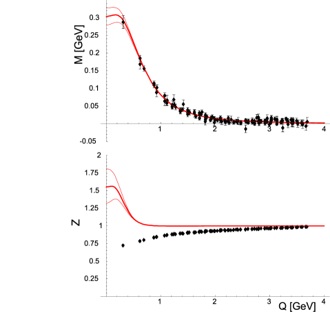
Figure 2: The dependence of the quark mass $M$ (top) and the wave function normalization $Z$ (bottom) on the Euclidean momentum $Q$ obtained from the meson dominance model with $d_{S}=5/2$. The lattice data, extrapolated to the chiral limit for the case of $M$, and taken at the current quark mass $\simeq 59$ MeV for the case of $Z$, are taken from Ref. Bowman et al. (2002a, b). The thicker lines correspond to optimum parameters of Eq. (169), while the thin lines indicate the uncertainty at the one-standard-deviation level.

The decrease of the quark mass as $1/Q^{3}$ at large Euclidean momenta is favored by recent lattice calculations Bowman et al. (2002a, b), where the fit to the functional form $c/((Q^{2})^{b}+(\Lambda^{2})^{b})$ is best when the parameter $b$ is close to 3 . We have performed a $\chi^{2}$ fit for $M(Q)$ of Eq. (164) to the data of Ref. Bowman et al. (2002a, b). These data, for the case of $M$, have been extrapolated to the chiral limit. We have treated $M_{S}$ and $M_{0}$ as free parameters. The $\chi^{2}$ fit results in the following optimum values,

$$M_{0} = 303\pm 24~{}{\rm MeV},$$

$$M_{S} = 970\pm 21~{}{\rm MeV},$$ (169)

with the optimum value of $\chi^{2}$ per degree of freedom equal to 0.72. The corresponding value of the quark condensate is

$$\langle\bar{q}q\rangle = -(243.0^{+0.1}_{-0.8}~{}{\rm MeV})^{3}.$$ (170)

The functions $M(Q)$ and $Z(Q)$, evaluated at optimum parameters, are shown in Fig. 2 with thick lines. The thin lines indicate the uncertainty at the one-standard-deviation level. The agreement with the data is very good for the case of $M$, and the $1/Q^{3}$ fall-off is clearly seen. In fact, fitting of the model with values of $d_{S}$ higher than $5/2$, which results in faster asymptotic decrease, results in a much worse agreement with the data. As seen from the bottom part of Fig. 2, for the case of $Z$ the agreement is not very good, but we should keep in mind the simplicity of the present model and the freedom in the scalar channel. For instance, the scalar spectral function can be multiplied, without loosing any of the general requirements, by an entire function. We also wish to stress that the optimum value of $\langle\bar{q}q\rangle$ obtained by fitting the model formulas to the lattice data agrees with the estimate (170).

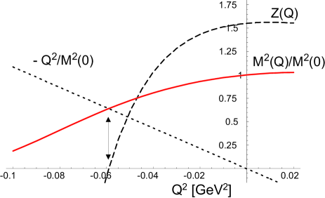
Figure 3: Square of the quark mass $M^{2}$ (solid line), minus the square of the Euclidean momentum $Q^{2}$ (dotted line), and the wave function normalization $Z$ (dashed line), plotted as functions of the square of Euclidean momentum, $Q^{2}$. The arrow indicates the point where $M^{2}=-Q^{2}$, but where also $Z=0$. As the result, the quark propagator has no pole. From the analyticity properties of $A$ and $B$ it follows that the quark propagator has no poles in the whole complex-$Q^{2}$ plane.

It is interesting to note that even though the mass function, $M(p^{2})$, presents a pole for time-like momenta, i.e. there exists a solution to the equation $M(p^{2})-p^{2}=0$, it does not correspond to a physical particle. This is because the normalization $Z(p^{2})$ also vanishes for the same value of $p^{2}$. This in fact is just a manifestation of the analyticity properties of $A(p)$ and $B(p)$ discussed above. Figure 3 shows the behavior of $M$ and $Z$ at low momenta. Arrows indicate the positions of the alleged pole in $M$, canceled by the zero of $Z$.

XIV Other predictions

The explicit model for the quark spectral function $\rho(\omega)$ allows for very simple and efficient evaluation of further interesting quantities. There is a whole bunch of predictions, from which we only list a few. The results decouple into those involving the vector spectral function, $\rho_{V}(\omega)$, and the scalar spectral function, $\rho_{S}(\omega)$. As stresses throughout the paper, all predictions are made for the model working scale $Q_{0}$, and the QCD evolution is needed if comparison to high-energy data is desired.

XIV.1 Pion transition form factor

According to the vector meson dominance model of the pion form factor, the transition form factor (VIII.3) becomes

$$F_{\pi\gamma^{\ast}\gamma^{\ast}}(Q^{2},A)=\frac{2f_{\pi}}{AN_{c}}\frac{1}{Q^{2}}\log\left[\frac{2M_{V}^{2}+(1+A)Q^{2}}{2M_{V}^{2}+(1-A)Q^{2}}\right]$$ (171)

$$+ \frac{16f_{\pi}M_{V}^{2}}{N_{c}[4M_{V}^{4}+4Q^{2}M_{V}^{2}+(1-A^{2})Q^{4}]}$$

As discussed in Sect. VIII, this expression provides the twist expansion, with the result of Eq. (LABEL:phin), but with VMD the log-moments of Eq. (150). The analysis and comparison to the data of Ref. CLEO Collaboration (1998) (J. Gronberg et al.) requires the QCD evolution of the higher twist components. This point will be analyzed elsewhere.

XIV.2 Pion light-cone wave function

Next, we use Eq. (156) in the expression for the pion light-cone wave function (108), with the result

$$\!\!\!\!\Psi(x,k_{\perp})=\frac{3M_{V}^{3}}{16\pi(k_{\perp}^{2}+M_{V}^{2}/4)^{5/2}}\theta(x)\theta(1-x).$$ (172)

Passing to the impact-parameter space with the Fourier-Bessel transform yields

$$\Psi(x,b) \equiv 2\pi\int_{0}^{\infty}k_{\perp}dk_{\perp}\Psi(x,k_{\perp})J_{0}(k_{\perp}b)$$ (173)

$$= \left(1+\frac{bM_{V}}{2}\right)\exp\left(-\frac{M_{V}b}{2}\right)\times$$

$$\theta(x)\theta(1-x).$$

The expansion at small $b$ yields

$$\Psi(x,b) = \left(1-\frac{M_{V}^{2}b^{2}}{8}+\frac{M_{V}^{3}b^{3}}{24}+\dots\right)$$ (174)

$$\times \theta(x)\theta(1-x).$$

The average transverse momentum squared is equal to

$$\langle k_{\perp}^{2}\rangle \equiv \frac{\int d^{2}k_{\perp}\,k_{\perp}^{2}\Psi(x,k_{\perp})}{\int d^{2}k_{\perp}\Psi(x,k_{\perp})}=-4\left.\frac{d\Psi(x,b)}{db^{2}}\right|_{b=0}$$ (175)

$$= \frac{M_{V}^{2}}{2},$$

which numerically gives $\langle k_{\perp}^{2}\rangle=(544~{}{\rm MeV})^{2}$ (all at the model working scale $Q_{0}$). This value is not far from the result of the Nambu–Jona-Lasinio model with the Pauli-Villars regularization, which produces $\langle k_{\perp}^{2}\rangle=(613~{}{\rm MeV})^{2}$ Arriola and Broniowski (2002). The estimates from QCD sum rules yield smaller values: one gets $(316{\rm MeV})^{2}$ based on Ref. Zhitnitsky (1994), and $(333\pm 40{\rm MeV})^{2}$ based on Ref. Belyaev and Ioffe (1982). One should note that these estimates are at $Q_{0}$ of the order of 1 GeV, hence the QCD evolution is needed to compare to our model results Arriola and Broniowski (2002).

XIV.3 Unintegrated pion structure function

Due to relation (133), exactly the same formulas as in the previous section hold for the unintegrated quark distribution function in the pion. Hence, we find

$$q(x,k_{\perp}) = \overline{q}(1-x,k_{\perp})$$

$$= \frac{3M_{V}^{3}}{16\pi(k_{\perp}^{2}+M_{V}^{2}/4)^{5/2}}\theta(x)\theta(1-x),$$

and the analogs of Eqs. (173-175).

XIV.4 Non-local quark condensate

The applications of Sect. XIV.2 and XIV.3 involved the vector spectral density. The scalar spectral density (158) enters the evaluation of the nonlocal condensate of Eq. (24). For $d_{S}=5/2$ we find immediately the interesting and simple result

$$Q(x)=\exp\left(-\frac{M_{S}\sqrt{-x^{2}}}{2}\right),$$ (177)

where $x$ denotes the Minkowski coordinate. For higher values of $d_{S}$ the expression is multiplied by a polynomial in the $x^{2}$ variable. Note the nonanalyticity in the $x^{2}$ variable in Eq. (177) as $x^{2}\to 0$. In the present model the moments of the quark condensate, Eq. (26), are well defined for $n<2d_{S}-4$, which means that for the preferred value of $d_{S}=5/2$ we may only consider the quark condensate itself, but not its moments. Nevertheless, the coordinate representation of the non-local condensate makes sense and can be given for the whole range of $x^{2}$.

XIV.5 Quark propagator in the coordinate representation

One may also pass to the coordinate representation for the $A$ and $B$ functions of Eq. (13), introducing

$$-i\hbox to0.0pt{\hbox to5.71527pt{\hfil/\hfil}\hss}xA(x) = \int\frac{d^{4}p}{(2\pi)^{4}}e^{-ip\cdot x}\hbox to0.0pt{\hbox to5.03125pt{\hfil/\hfil}\hss}pA(p),$$

$$B(x) = \int\frac{d^{4}p}{(2\pi)^{4}}e^{-ip\cdot x}B(p).$$ (178)

With straightforward algebra one finds

$$A(x) = \frac{48+24M_{V}\sqrt{-x^{2}}-6M_{V}^{2}x^{2}+M_{V}^{3}(-x^{2})^{3/2}}{96\pi^{2}x^{4}}$$

$$\times e^{-M_{V}\sqrt{-x^{2}}/2},$$

$$B(x) = \frac{2^{3-2d_{S}}\langle\overline{q}q\rangle}{N_{c}\Gamma(d_{S}-2)}(M_{S}\sqrt{-x^{2}})^{d_{S}-2}K_{2-d_{S}}(M_{S}\sqrt{-x^{2}}/2),$$

where $x$ denotes the Minkowski coordinate. We have used $d_{V}=5/2$. In the limit of low $x$ one recovers the result of the free theory, $A(x)\simeq 1/(2\pi^{2}x^{4})$. For the preferred value of $d_{S}=5/2$ we find that

$$B(x)=\langle\overline{q}q\rangle/(4N_{c})\exp(-M_{S}\sqrt{-x^{2}}/2),$$ (180)

in agreement with Eq. (177).

Table 1: Summary of conditions for the quark spectral function $\rho(\omega)$.

Spectral condition	Physical significance
normalization
$\rho_{0}=1$	proper normalization of the quark propagator
	preservation of anomalies
	proper normalization of the pion distribution amplitude
	proper normalization of the pion structure function
	reproduction of the large-$N_{c}$ quark-model values of the Gasser-Leutwyler coefficients
	relation $M_{V}^{2}=24\pi^{2}f_{\pi}^{2}/N_{c}$ in the vector-meson dominance model
positive moments
$\rho_{1}=0$	vanishing quark mass at asymptotic Euclidean momenta, $M(Q^{2})\to 0$
$\rho_{2}=0$	finiteness of the pion decay constant, $f_{\pi}$
$\rho_{3}=0$	finiteness of the quark condensate, $\langle\bar{q}q\rangle$
$\rho_{4}=0$	finiteness of the vacuum energy density, $B$
$\rho_{n}=0,\qquad n=2,4,\dots$	factorization in the twist expansion of vector amplitudes
$\rho_{n}=0,\qquad n=5,7,\dots$	finiteness of $\langle\bar{q}(\partial^{2})^{(n-3)/2}q\rangle$
	factorization in the twist expansion of the scalar pion form factor
negative moments
$\rho_{-2}>0$	positive value of the quark wave-function normalization at vanishing momentum, $Z(0)>0$
$\rho_{-1}/\rho_{-2}>0$	positive value of the quark mass at vanishing momentum, $M(0)>0$
$\rho_{-n}$	low-momentum expansion of correlators
positive log-moments
$\rho^{\prime}_{2}<0$	$f_{\pi}^{2}=-N_{c}/(4\pi^{2})\rho^{\prime}_{2}$
$\rho^{\prime}_{3}>0$	negative value of the quark condensate, $\langle\bar{q}q\rangle=-N_{c}/(4\pi^{2})\rho^{\prime}_{3}$
$\rho^{\prime}_{4}>0$	negative value of the vacuum energy density, $B=-N_{c}/(4\pi^{2})\rho^{\prime}_{4}$
$\rho^{\prime}_{5}<0$	positive value of the squared vacuum virtuality of the quark, $\lambda^{2}_{q}=-\rho^{\prime}_{5}/\rho^{\prime}_{3}$
$\rho^{\prime}_{n}$	high-momentum (twist) expansion of correlators

XV Conclusion and final remarks

In the present work we have developed a chiral quark model, which tries to incorporate as many known features based on chiral symmetry and the partonic quark substructure of hadrons as possible. This approach, first unveiled in Ref. Arriola (2001), should be considered as a simple prototype of a construction which may be certainly improved in many respects. Taking into account the fact that the emerging picture is very encouraging, economic, and predictive, we believe that applications and extensions of the model deserve a thorough further investigation.

The key ingredient is the use of a generalized spectral representation for the quark propagator combined with the gauge technique for constructing the vertices involving quarks and currents. The generalized Lehmann representation implies analyticity properties of the quark propagator on the complex plane but positivity or reality are abandoned. In particular, the analytic continuation from the Euclidean to the Minkowski space back and forth becomes straightforward. We remind that this continuation is explicitly used when computing hadronic matrix elements in momentum space. The possibility of doing this continuation becomes extremely convenient when dealing with calculations of soft matrix elements of high-energy processes. In a purely Euclidean formulation one stays in the coordinate space and the extraction of the parton distribution functions or amplitudes is often limited in practice to the few lowest moments.

The conditions used to constrain the spectral function are collected in Table I. Finiteness and factorization enforce the vanishing of the positive moments, while a number of available experimental observables can be used to fix the values and signs of the negative moments and the log-moments.

Instead of making a specific model for the propagator based on extrapolations from the Euclidean region to the complex plane we devise an infinite set of spectral conditions based on the requirement that our model produces finite hadronic observables. As a result the high energy behavior of certain matrix elements corresponds to a pure twist expansion, with no logarithmic behavior. This is consistent with the interpretation that the model is defined at a low renormalization point $Q_{0}$. Thus, our model results should be considered as initial condition for the QCD evolution, hence automatically incorporating the correct high energy radiative corrections to hadronic observables. The low renormalization point $Q_{0}$ is determined by the analysis of two different processes: the pion transition form factor and the pion structure functions. We find compatible values in the range $Q_{0}\sim 300{\rm MeV}$, corresponding to $\alpha(Q_{0})/(2\pi)\sim 0.3$. For the model scale, the leading twist contribution for the pion structure function and the pion distribution amplitude coincide and are equal to one, $q(x)=\varphi_{\pi}(x)=1$, regardless of the spectral function. At the same time the correct anomalous form factor for the process $\pi^{0}\to\gamma\gamma$ is obtained. This resolves the conflict between proper low-energy and high-energy normalization of the pion transition form factor. The QCD evolution of both the PDF and PDA has been shown to provide a very reasonable agreement with the data analysis.

The pion form factor does depend on the spectral function. Further interesting analytic relations can be obtained by determining the even contribution to the spectral function from the requirement that the pion form factor has the vector meson dominance form, which is known to describe experimental data in the available momentum range very well. As a result, the vector meson mass becomes proportional to the pion weak decay constant. The vector contribution to the spectral function exhibits a pole at the origin and non-integrable branch points at plus or minus the vector meson mass. As a consequence the spectral function must be interpreted as a distribution centered at the branch points.

The form of the spectral function suggested by the vector channel can be also used with minor modifications for the scalar channel. This way the full quark propagator can be studied and its analytic structure analyzed: there are no poles all over the complex plane, only cuts located at the branch points of the spectral function. Moreover, the asymptotic behavior in the Euclidean region reflects this cut structure by a half-integer power fall-off of the quark mass function in the squared Euclidean momentum $Q^{2}$. The recent lattice data Bowman et al. (2002a, b) set this half integer power to $3/2$ quite unambiguously. Fixing this power leaves only the quark mass function at the origin (the constituent quark mass) and the quark condensate as free parameters. The fit to the data for the mass function, $M(p^{2})$, is very good and the values for both the condensate and the constituent quark mass at $p^{2}=0$ agree with other estimates. The fit to the quark wave-function normalization, $Z(p^{2})$, is not nearly as good as for $M(p^{2})$, leaving room for improvement.

Possible extensions of the general model involve the inclusion of more general solutions of the Ward-Takahashi identities. The meson-dominance model can be improved by studying more general forms of the scalar quark spectral function. Moreover, the inclusion of finite quark masses would allow the extension of the present model to the complete pseudoscalar octet. These issues are under investigation.

Appendix A One-loop integrals

A.1 Two-point integral

The two-point one loop integral regularized in $4+\epsilon$ dimensions is

$$\!\!\!\!\!\!\!\!I(q^{2},\omega)=\frac{1}{i}\int{d^{4}k\over(2\pi)^{4}}{1\over k^{2}-\omega^{2}+i0^{+}}{1\over(q-k)^{2}-\omega^{2}+i0^{+}}$$

$$\!\!\!\!\!\!\!\!=\frac{1}{16\pi^{2}}\left(2+\sqrt{1-{4\omega^{2}\over q^{2}}}\log{\sqrt{1-{4\omega^{2}\over q^{2}}}-1\over\sqrt{1-{4\omega^{2}\over q^{2}}}+1}\right)+I(0,\omega),$$

with

$$I(0,\omega)=-\frac{1}{16\pi^{2}}\left(\frac{1}{\epsilon}+\log(\omega^{2}/\mu^{2})\right).$$ (182)

We also introduce

$$\bar{I}(q^{2},\omega)\equiv I(q^{2},\omega)-I(0,\omega).$$ (183)

In the Feynman parametric form we equivalently have

$$I(q^{2},\omega) = -\frac{1}{(4\pi)^{2}}\int d\omega\rho(\omega)$$ (184)

$$\times \int_{0}^{1}dx\log\left[\omega^{2}+x(1-x)q^{2}\right].$$

The imaginary part yields

$$\frac{1}{\pi}{\rm Im}I(q^{2},\omega)=\frac{1}{16\pi^{2}}\sqrt{1-\frac{\omega^{2}}{4q^{2}}}\theta(q^{2}-4\omega^{2}).$$ (185)

Thus the once-subtracted dispersion relation,

$$\bar{I}(q^{2},\omega)=\frac{q^{2}}{\pi}\int_{4w^{2}}^{\infty}\frac{dt}{t}\,\frac{{\rm Im}I(t,\omega)}{t-q^{2}-i0^{+}},$$ (186)

holds. The asymptotic behavior for large Euclidean $-q^{2}$ is

$$\!\!\!\!\!I(q^{2},\omega)=\frac{1}{16\pi^{2}}\{2-\frac{1}{\epsilon}-\log(-q^{2}/\mu^{2})+$$ (187)

$$\!\!\!\!\!\frac{2\omega^{2}}{q^{2}}\left[\log(-q^{2}/\omega^{2})+1\right]+\frac{2\omega^{4}}{q^{4}}\left[\log(-q^{2}/\omega^{2})-\frac{1}{2}\right]\dots\}.$$

At low $q^{2}$ we have

$$\bar{I}(q^{2},\omega)=\frac{1}{16\pi^{2}}\left\{\frac{q^{2}}{6\omega^{2}}+\frac{q^{4}}{60\omega^{4}}+\frac{q^{6}}{420\omega^{6}}+\dots\right\}.$$ (188)

A.2 Three-point integral

The three-point one-loop integral is defined as

$$K((q_{1}-q_{2})^{2},q_{1}^{2},q_{2}^{2},\omega)=\frac{1}{i}\int{d^{4}k\over(2\pi)^{4}}{1\over k^{2}-\omega^{2}+i0^{+}}\times$$

$${1\over(k-q_{1})^{2}-\omega^{2}+i0^{+}}{1\over(k-q_{2})^{2}-\omega^{2}+i0^{+}}.$$

We analyze it with the dimensional regularization, and for the case where the virtuality of one of the external line vanishes, $(q_{1}-q_{2})^{2}=0$ (massless pion). We immediately find the result

$$K(0,0,0,\omega)=-\frac{1}{16\pi^{2}}\frac{1}{2\omega^{2}}.$$ (190)

The following Feynman parameterization is useful:

$$\frac{1}{abc}=2\int_{0}^{1}dx\int_{0}^{1}dy\frac{x}{[xya+x(1-y)b+(1-x)c]^{3}}.$$ (191)

Carrying the momentum integration and introducing $z=2y-1$ yields

$$K(0,\frac{1+A}{2}q^{2},\frac{1-A}{2}q^{2},\omega)=\frac{1}{16\pi^{2}}\int_{0}^{1}dx\int_{-1}^{1}dz\times$$

$$\frac{x}{(1-x)x(1+Az)q^{2}-2\omega^{2}}.$$ (192)

At $A=0$ we find

$$K(0,\frac{1}{2}q^{2},\frac{1}{2}q^{2},\omega)=$$ (193)

$$\frac{1}{16\pi^{2}}\frac{2}{q^{2}\sqrt{1-8\omega^{2}/q^{2}}}\log\frac{1+\sqrt{1-8w^{2}/q^{2}}}{1-\sqrt{1-8w^{2}/q^{2}}}.$$

At low $q^{2}$ the expansion is

$$K(0,\frac{1}{2}q^{2},\frac{1}{2}q^{2},\omega)=$$ (194)

$$-\frac{1}{16\pi^{2}}\left[\frac{1}{2\omega^{2}}+\frac{q^{2}}{24\omega^{4}}+\frac{q^{4}}{240\omega^{4}}+...\right],$$

and an high $q^{2}$

$$K(0,\frac{1}{2}q^{2},\frac{1}{2}q^{2})=-\frac{1}{16\pi^{2}}\left[2\log\left(-2\omega^{2}/q^{2}\right)\frac{1}{q^{2}}\right.$$

$$\left.-8\left[\log\left(-2\omega^{2}/q^{2}\right)+1\right]\frac{\omega^{2}}{q^{4}}+...\right].$$ (195)

The integral over $x$ in Eq. (192) yields

$$K(0,\frac{1+A}{2}q^{2},\frac{1-A}{2}q^{2},\omega)=$$ (196)

$$\frac{1}{16\pi^{2}}\int_{-1}^{1}dz\frac{1}{(1+Az)q^{2}s}\log\frac{1+s}{1-s},$$

$$s=\sqrt{1-8\omega^{2}/(q^{2}(1+Az))}.$$

At low $q^{2}$ we have

$$K(0,\frac{1+A}{2}q^{2},\frac{1-A}{2}q^{2},\omega)=$$ (197)

$$-\frac{1}{16\pi^{2}}\left[\frac{1}{2\omega^{2}}+\frac{q^{2}}{24\omega^{4}}+\frac{(A^{2}+3)q^{4}}{720\omega^{4}}+...\right],$$

The large-$q^{2}$ expansion produces

$$K(0,\frac{1+A}{2}q^{2},\frac{1-A}{2}q^{2},\omega)$$ (198)

$$=-\frac{1}{16\pi^{2}}\int_{-1}^{1}dz\left\{\frac{1}{q^{2}(1+Az)}\log\left(-\frac{2\omega^{2}}{q^{2}(1+Az)}\right)\right.$$

$$\left.+\frac{4\omega^{2}}{q^{4}(1+Az)^{2}}\left[\log\left(-\frac{2\omega^{2}}{q^{2}(1+Az)}\right)+1\right]+....\right\}$$

The integral over $z$ in Eq. (196) gives finally the simple general result

$$K(0,\frac{1+A}{2}q^{2},\frac{1-A}{2}q^{2})$$

$$=\frac{1}{32\pi^{2}Aq^{2}}\left[\left(\log\frac{1+s_{+}}{1-s_{+}}\right)^{2}-\left(\log\frac{1+s_{-}}{1-s_{-}}\right)^{2}\right],$$

$$s_{\pm} = \sqrt{1-8\omega^{2}/(q^{2}(1\pm A))}.$$

Appendix B Discontinuity in the Bjorken limit

Let us consider the one-loop function

$$T(p,q) = i\int{d^{4}k\over(2\pi)^{4}}{1\over[(k-p)^{2}-\omega^{2}+i0^{+}]^{2}}\times$$

$${1\over k^{2}-\omega^{2}+i0^{+}}{1\over(q-k-p)^{2}-\omega^{2}+i0^{+}}.$$

The discontinuity in the $s=(p+q)^{2}$ channel may be computed through the Cutkosky rules,

$${\rm Disc}\,T(p,q)=i\int{d^{4}k\over(2\pi)^{4}}{1\over[(k-p)^{2}-\omega^{2}+i0^{+}]^{2}}$$

$$(-2\pi i)^{2}\delta^{+}(k^{2}-\omega^{2})\delta^{+}[(q-k-p)^{2}-\omega^{2}].$$ (201)

We choose the reference frame of the target at rest

$$p=(m,\mathchoice{\mbox{\boldmath$\displaystyle 0$}}{\mbox{\boldmath$\textstyle 0$}}{\mbox{\boldmath$\scriptstyle 0$}}{\mbox{\boldmath$\scriptscriptstyle 0$}}_{\perp},0),\;q=(q_{0},\mathchoice{\mbox{\boldmath$\displaystyle 0$}}{\mbox{\boldmath$\textstyle 0$}}{\mbox{\boldmath$\scriptstyle 0$}}{\mbox{\boldmath$\scriptscriptstyle 0$}}_{\perp},q_{3}),\;q^{2}=-Q^{2}=q_{0}^{2}-\mathchoice{\mbox{\boldmath$\displaystyle q$}}{\mbox{\boldmath$\textstyle q$}}{\mbox{\boldmath$\scriptstyle q$}}{\mbox{\boldmath$\scriptscriptstyle q$}}^{2}.$$

One gets then

$$q_{0} = \frac{Q^{2}}{2m_{\pi}x},$$ (203)

$$q_{3} = \frac{Q^{2}}{2m_{\pi}x}\sqrt{1+\frac{4m_{\pi}^{2}x^{2}}{Q^{2}}}\to\frac{Q^{2}}{2m_{\pi}x}+m_{\pi}x+\dots$$

In the light-cone coordinates, defined as

$$k^{+} = k^{0}+k^{3},\;k^{-}=k^{0}-k^{3},\;\mathchoice{\mbox{\boldmath$\displaystyle k$}}{\mbox{\boldmath$\textstyle k$}}{\mbox{\boldmath$\scriptstyle k$}}{\mbox{\boldmath$\scriptscriptstyle k$}}_{\perp}=(k^{1},k^{2}),$$

$$dk^{0}dk^{3} = \frac{1}{2}dk^{+}dk^{-},$$ (204)

one obtains

$$q^{+} = q^{0}+q^{3}\to\frac{Q^{2}}{m_{\pi}x},$$

$$q^{-} = q^{0}-q^{3}\to-m_{\pi}x,$$ (205)

and also

$$\delta^{+}\left[(k-p-q)^{2}-\omega^{2}\right]\to\frac{m_{\pi}x}{Q^{2}}\delta\left[k^{-}-(1-x)m_{\pi}\right],$$

$$\delta^{+}\left[k^{2}-\omega^{2}\right]\to\frac{1}{m_{\pi}(1-x)}\delta\left[k^{+}-\frac{\mathchoice{\mbox{\boldmath$\displaystyle k$}}{\mbox{\boldmath$\textstyle k$}}{\mbox{\boldmath$\scriptstyle k$}}{\mbox{\boldmath$\scriptscriptstyle k$}}_{\perp}^{2}+\omega^{2}}{m_{\pi}(1-x)}\right].$$

Thus finally we get

$${\rm Im}T(p,q)\to$$ (207)

$$\frac{x(1-x)}{Q^{2}}\int\frac{d^{2}\mathchoice{\mbox{\boldmath$\displaystyle k$}}{\mbox{\boldmath$\textstyle k$}}{\mbox{\boldmath$\scriptstyle k$}}{\mbox{\boldmath$\scriptscriptstyle k$}}_{\perp}}{(2\pi)^{2}}\frac{1}{\left[\mathchoice{\mbox{\boldmath$\displaystyle k$}}{\mbox{\boldmath$\textstyle k$}}{\mbox{\boldmath$\scriptstyle k$}}{\mbox{\boldmath$\scriptscriptstyle k$}}_{\perp}^{2}+\omega^{2}-m_{\pi}^{2}x(1-x)]\right]^{2}}.$$

References

- Vogl and Weise (1991) U. Vogl and W. Weise, Prog. Part. Nucl. Phys. 27, 195 (1991).
- Klevansky (1992) S. P. Klevansky, Rev. Mod. Phys. 64, 649 (1992).
- Volkov (1993) M. K. Volkov, Part. and Nuclei B24, 1 (1993).
- Hatsuda and Kunihiro (1994) T. Hatsuda and T. Kunihiro, Phys. Rep. 247, 221 (1994).
- Christov et al. (1996) C. V. Christov, A. Blotz, H.-C. Kim, P. Pobylitsa, T. Watabe, T. Meissner, E. Ruiz Arriola, and K. Goeke, Prog. Part. Nucl. Phys. 37, 91 (1996).
- Alkofer et al. (1996) R. Alkofer, H. Reinhardt, and H. Weigel, Phys. Rep. 265, 139 (1996).
- Ripka (1997) G. Ripka, Quarks Bound by Chiral Fields (Clarendon Press, Oxford, 1997).
- Ruiz Arriola (2002) E. Ruiz Arriola, Acta Phys. Pol. B33, 4443 (2002).
- Itzykson and Zuber (1980) C. Itzykson and J. B. Zuber, Quantum Field Theory (McGraw-Hill, New York, 1980).
- Delbourgo and West (1977) R. Delbourgo and P. C. West, J. Phys. A10, 1049 (1977).
- Delbourgo (1979) R. Delbourgo, Nuovo Cimento A49 (1979).
- Arriola (2001) E. Ruiz Arriola, in proceedings of the Workshop on Lepton Scattering, Hadrons and QCD, Adelaide, Australia, 2001, edited by W. Melnitchouk, A. Schreiber, P. Tandy, and A. W. Thomas (World Scientific, Singapore, 2001), hep-ph/0107087.
- Jaffe and Ross (1980) R. L. Jaffe and G. C. Ross, Phys. Lett. B93, 313 (1980).
- Jaffe (1986) R. L. Jaffe, in proceedings of the Los Alamos School, 1985, edited by M. B. Johnson and A. Picklesimer (Wiley, New York, 1986).
- Davidson and Arriola (1995) R. M. Davidson and E. Ruiz Arriola, Phys. Lett. B359, 273 (1995).
- Davidson and Arriola (2002) R. M. Davidson and E. Ruiz Arriola, Act. Phys. Pol. B33, 1791 (2002).
- Arriola and Broniowski (2002) E. Ruiz Arriola and W. Broniowski, Phys. Rev D66, 094016 (2002).
- Bowman et al. (2002a) P. O. Bowman, U. M. Heller, and A. G. Williams, Phys. Rev. D66, 014505 (2002a).
- Bowman et al. (2002b) P. O. Bowman, U. M. Heller, D. B. Leinweber, and A. G. Williams (2002b), eprint hep-lat/0209129.
- Haeri (1988) B. Haeri, Phys. Rev. D38, 3799 (1988).
- Lee and Wick (1969) T. D. Lee and G. C. Wick, Nucl. Phys. B9, 209 (1969).
- Cutkosky et al. (1969) R. E. Cutkosky, P. V. Landshoff, D. I. Olive, and J. Polkinghorne, Nucl. Phys. B12, 281 (1969).
- Boulware and Gross (1984) D. G. Boulware and D. J. Gross, Nucl. Phys. B233, 1 (1984).
- Praszałowicz and Rostworowski (2001) M. Praszałowicz and A. Rostworowski, Phys. Rev. D64, 074003 (2001).
- Ioffe (2002) B. L. Ioffe, Tech. Rep. (2002), eprint hep-ph/0207191.
- Mikhailov and Radyushkin (1989) S. V. Mikhailov and A. V. Radyushkin, Sov. J. Nucl. Phys. 49, 494 (1989).
- Mikhailov and Radyushkin (1992) S. V. Mikhailov and A. V. Radyushkin, Phys. Rev. D45, 1754 (1992).
- Bakulev and Mikhailov (2002) A. P. Bakulev and S. V. Mikhailov, Phys. Rev. D65, 114511 (2002).
- Dorokhov and Broniowski (2002) A. E. Dorokhov and W. Broniowski, Phys. Rev. D65, 094007 (2002).
- Belyaev and Ioffe (1982) V. M. Belyaev and B. L. Ioffe, Sov. Phys. JETP 56, 493 (1982).
- Ioffe and Zyablyuk (2002) B. L. Ioffe and K. N. Zyablyuk, Tech. Rep. (2002), eprint hep-ph/0207183.
- Renner (1968) B. Renner, Current Algebras and Their Applications (Pergamon Press, New York, 1968).
- Delbourgo (1999) R. Delbourgo, Austral. J. Phys. 52, 681 (1999).
- Sauli (2002) V. Sauli, Tech. Rep. (2002), eprint hep-ph/0209046.
- Broniowski et al. (1996) W. Broniowski, G. Ripka, E. N. Nikolov, and K. Goeke, Zeit. Phys. A 354, 421 (1996).
- Pagels and Stokar (1979) H. Pagels and S. Stokar, Phys. Rev. D20, 2947 (1979).
- Weinberg (1967) S. Weinberg, Phys. Rev. Lett. 18, 507 (1967).
- C. Bernard and Weinberg (1975) J. L. C. Bernard, A. Duncan and S. Weinberg, Phys. Rev. D12, 792 (1975).
- Broniowski (1999) W. Broniowski (1999), eprint hep-ph/9911204.
- Tarrach (1979) R. Tarrach, Z. Phys. C2, 221 (1979).
- Faccioli et al. (2002) P. Faccioli, A. Schwenk, and E. V. Shuryak (2002), eprint hep-ph/0202027.
- et al. (1976) C. J. B. et al., Phys. Rev. Lett 37, 1693 (1976).
- Volmer et al. (2001) J. Volmer et al. (The Jefferson Lab F(pi)), Phys. Rev. Lett. 86, 1713 (2001), eprint nucl-ex/0010009.
- Blok et al. (2002) H. P. Blok, G. M. Huber, and D. J. Mack (2002), nucl-ex/0208011.
- Amendolia et al. (1986) S. R. Amendolia et al. (NA7), Nucl. Phys. B277, 168 (1986).
- Lepage and Brodsky (1980) G. P. Lepage and S. J. Brodsky, Phys. Rev. D22, 2157 (1980).
- Dorokhov (2002a) A. E. Dorokhov (2002a), talk presented at the 37th Rencontres de Moriond on QCD and Hadronic Interactions, Les Arcs, France, 16-23 March 2002, hep-ph/0206088.
- Dorokhov (2002b) A. E. Dorokhov, Pis’ma ZhETF 77, 68 (2002b).
- Müller (1995) D. Müller, Phys. Rev. D51, 3855 (1995).
- Schmedding and Yakovlev (2000) A. Schmedding and O. Yakovlev, Phys. Rev. D62, 116002 (2000).
- Bakulev et al. (2002) A. P. Bakulev, S. V. Mikhailov, and N. G. Stefanis (2002), eprint hep-ph/0212250.
- CLEO Collaboration (1998) (J. Gronberg et al.) CLEO Collaboration (J. Gronberg et al.), Phys. Rev. D57, 33 (1998).
- Adler (1971) S. L. Adler, Phys. Rev. D4, 3497 (1971).
- Terent’ev (1972) M. V. Terent’ev, Phys. Lett. 38B, 419 (1972).
- Aviv and Zee (1972) R. Aviv and A. Zee, Phys. Rev. D5, 2372 (1972).
- Weigel et al. (1999) H. Weigel, E. Ruiz Arriola, and L. Gamberg, Nucl. Phys. B560, 383 (1999).
- Ellis (1976) J. R. Ellis (1976), in Les Houches 1976, Proceedings, Weak and Electromagnetic Interactions At High Energies, Amsterdam 1977, 1-114 and Preprint - ELLIS J (76,REC.JAN 77) 171p.
- Altarelli and Parisi (1977) G. Altarelli and G. Parisi, Nucl. Phys. B126, 298 (1977).
- Sutton et al. (1992) P. J. Sutton, A. D. Martin, R. G. Roberts, and W. J. Stirling, Phys. Rev. D45, 2349 (1992).
- Gasser and Leutwyler (1984) J. Gasser and H. Leutwyler, Ann. Phys. 158, 142 (1984).
- Gasser and Leutwyler (1985) J. Gasser and H. Leutwyler, Nucl. Phys. B250, 465 (1985).
- Chan (1986) L.-H. Chan, Phys. Rev. Lett. 57, 1199 (1986).
- Arriola (1991) E. Ruiz Arriola, Phys. Lett. B253, 430 (1991).
- Schuren et al. (1992) C. Schuren, E. Ruiz Arriola, and K. Goeke, Nucl. Phys. A547, 612 (1992).
- Zhitnitsky (1994) A. R. Zhitnitsky, Phys. Lett. B329, 493 (1994).
- Gel’fand and Shilov (1964) I. M. Gel’fand and G. E. Shilov, Generalized Functions, vol. 1 (Academic, New York, 1964).