Simulation of Atmospheric Muon and Neutrino Fluxes with CORSIKA

Abstract

The fluxes of atmospheric muons and neutrinos are calculated by a three dimensional Monte Carlo simulation with the air shower code CORSIKA using the hadronic interaction models DPMJET, VENUS, GHEISHA, and UrQMD. For the simulation of low energy primary particles the original CORSIKA has been extended by a parametrization of the solar modulation and a microscopic calculation of the directional dependence of the geomagnetic cut-off functions. An accurate description for the geography of the Earth has been included by a digital elevation model, tables for the local magnetic field in the atmosphere, and various atmospheric models for different geographic latitudes and annual seasons. CORSIKA is used to calculate atmospheric muon fluxes for different locations and the neutrino fluxes for Kamioka. The results of CORSIKA for the muon fluxes are verified by an extensive comparison with recent measurements. The obtained neutrino fluxes are compared with other calculations and the influence of the hadronic interaction model, the geomagnetic cut-off and the local magnetic field on the neutrino fluxes is investigated.

I Introduction

Atmospheric neutrinos are produced by the interaction of the primary cosmic radiation with the Earth’s atmosphere. They result mainly from the decay of the charged pions and muons:

$$\pi^{+}\,\,\,\rightarrow \mu^{+}+\nu_{\mu}$$

$$\hskip 5.69046pt\hookrightarrow e^{+}+\nu_{e}+\overline{\nu_{\mu}}$$

$$\pi^{-}\,\,\,\rightarrow \mu^{-}+\overline{\nu_{\mu}}$$

$$\hskip 5.69046pt\hookrightarrow e^{-}+\overline{\nu_{e}}+\nu_{\mu},$$

and to about 10 % from similar reaction chains for kaons. A simple balancing of the different neutrino species involved results in the following approximate relations between the numbers of neutrinos:

$$\frac{\,\nu_{e}\,}{\overline{\nu_{e}}}=\frac{\mu^{+}}{\mu^{-}},\hskip 22.76228pt\frac{\,\nu_{\mu}\,}{\overline{\nu_{\mu}}}=1,\hskip 8.5359pt{\rm and}\hskip 8.5359pt\frac{\nu_{\mu}+\overline{\nu_{\mu}}}{\,\nu_{e}+\overline{\nu_{e}}\,}=2.$$ (2)

A more detailed calculation leads to an energy dependence of all the ratios. Especially the ratio of muon neutrinos to electron neutrinos strongly depends on the energy, because the number of muons reaching sea-level before decaying increases with the energy.

A precise simulation of atmospheric neutrino fluxes is of essential interest for the interpretation of the so-called atmospheric neutrino anomaly, i.e. the observation of several neutrino detectors Fukuda et al. (1998a, b); Becker-Szendy et al. (1992); Hirata et al. (1992); Allison et al. (1997); Kafka (1999) that the ratio of muon neutrinos to electron neutrinos in the atmosphere differs approximately by a factor of 2 from the theoretical predictions. The flux of electron neutrinos seems to agree relatively well with the expectation, and the anomaly results mainly from a lack of muon neutrinos.

In addition, the anomaly displays a pronounced dependence on the angle of incidence. The highest deficit is measured for neutrinos traveling through the Earth for entering the detectors in upward direction, while for downward going neutrinos agreement with the theory is found. This directional dependence of the anomaly is commonly interpreted in terms of neutrino oscillations.

Due to the enormous size of the detector, the results obtained by the Super-Kamiokande experiment near Kamioka, Japan are statistically most significant and allow a most detailed exploration of the anomaly. As only detector so far, Super-Kamiokande could establish a pronounced East-West-effect in the neutrino flux originating from the influence of the Earth’s magnetic field on the trajectories of the charged primary and secondary cosmic ray particles Futagami et al. (1999).

Table 1: Features of the different models applied in the calculation of atmospheric neutrino fluxes. The following abbreviations are used in the table: IGRF stands for the International Geomagnetic Reference Field IAGA Division V, Working Group 8, AOS (1992), WMM for the World Magnetic Field Model MacMillan et al. (1997); Quinn et al. (1997), and USSA for the US Standard Atmosphere Forsythe (1969). The terms used in the table are explained in Sec. II.

	BGS	BN	HKHM	LBK	TKNW	BFLMSR	HKKM	Ply
Hadronic interaction	TARGET	semi-	FRITIOF/	TARGET	GEANT	FLUKA	FRITIOF/NUCRIN	GEANT
model		analytical	NUCRIN				DPMJET III
							(parametrized)
Dimensions	1	1	1	3	3	3	3	3
Directional dependence	dipole	dipole-	IGRF	dipole	IGRF	IGRF	dipole	WMM
of geomagnetic cut-off		like
Penumbra of cut-off	no	no	no	no	yes	yes	no	yes
Local magnetic field	no	no	no	no	yes	no	yes	yes
Energy loss by ionization	yes	yes	yes	yes	yes	yes	yes	yes
Multiple scattering of muons	no	no	no	no	yes	yes	yes	yes
Atmospheric model	USSA	Dorman	USSA	?	USSA	USSA	USSA	USSA
		model
Elevation model of the	no	no	no	no	no	no	no	no
Earth

The fluxes of atmospheric neutrinos have been calculated with various theoretical approaches invoking different hadronic interaction models. Detailed calculations have been done by Barr, Gaisser, and Stanev (BGS) Gaisser et al. (1988); Barr et al. (1989); Agrawal et al. (1996); Bugaev and Naumov (BN) Bugaev and Naumov (1989); Honda, Kasahara, Hidaka, and Midorikawa (HKHM) Honda et al. (1990, 1995); Lee, Bludman, and Koh (LBK) Lee and Bludman (1988); Lee and Koh (1990), Tserkovnyak, Komar, Nally, and Waltham (TKNW) Tserkovnyak et al. (1999, 2001); Battistoni, Ferrari, Lipari, Montaruli, Sala, and Rancati (BFLMSR) Battistoni et al. (2000); Battistoni (2001); Battistoni et al. (2002); Honda, Kajita, Kasahara, and Midorikawa (HKKM) Honda et al. (2001a, b); and Plyaskin (Ply) Plyaskin (2001). A recent review of the calculations of atmospheric neutrinos can be found in Ref. Gaisser and Honda (2002).

The calculation of BGS is a one dimensional Monte Carlo simulation made in two steps. First, cascades for different primary energies and zenith angles are simulated, and subsequently, the energy depending yields of the secondary particles are weighted by the primary spectrum and the geomagnetic cut-off characteristics for the detector location. The hadronic interactions are described with TARGET Gaisser et al. (1983), a parametrization of accelerator data with special emphasis on energies around 20 GeV.

The BN calculation is based on a one dimensional semi-classical integration of the atmospheric cascade equations in straight forward approximation over the primary spectrum. The hadronic interaction is described by an analytical parametrization of double differential inclusive cross-sections based on a compilation of accelerator data. This approach neglects many details on the nature of the hadronic interaction .

The HKHM calculation is made by using the air shower simulation code COSMOS Kasahara (1995) in a one dimensional Monte Carlo simulation. For energies above 5 GeV the hadronic interaction is described in the frame of FRITIOF version 1.6 Nilsson-Almqvist and Stenlund (1987) with JETSET 6.3 Sjöstrand and Bengtsson (1987). At lower energies NUCRIN is used Hänßgen and Ranft (1986).

The model applied in the LBK calculations is the model of BGS, but extending the calculation on three dimensions. The same primary spectrum has been used, too. The calculation intends to study the influence of the transversal momenta in the different reactions on the neutrino fluxes.

The three dimensional calculation of TKNW is based on the GEANT 3.21 detector simulation tool gea (1993) and its various models for the hadronic interaction, CALOR Bertini (1963, 1970, 1972), FLUKA92 Aarnio et al. (1993); Fasso et al. (1993), and GHEISHA Fesefeldt (1985).

Both, the LBK and the TKNW calculation failed to discover a major enhancement of the neutrino fluxes near the horizon, which was predicted for the first time in the three dimensional simulation of BFLMSR. In the meantime, the TKNW group revised its model, and finds also an enhancement at the horizon Tserkovnyak et al. (2001).

In the calculations of BFLMSR the FLUKA98 and FLUKA2000 Fasso et al. (2000a, b) are used as models for the hadronic interaction. These versions of FLUKA are quite different from the FLUKA92 version integrated in the GEANT package and being used in the TKNW calculation.

HKKM extended the calculation of HKHM to three dimensions. Additionally, the interaction models of COSMOS can be replaced now by a parametrized version of DPMJET III Roesler et al. (2000). Meaning that instead of interfacing DPMJET to COSMOS, DPMJET is run at fixed energies and the yields of secondary particles are parametrized. This enhances very much the calculation speed, but subtile details of the interaction model might be lost in this approach. The published results being used in this paper for comparisons are based on the hadronic interaction models of the original COSMOS.

The calculation of Plyaskin is based also on the GEANT detector simulation package, but only the GHEISHA model is used for the simulation of the hadronic interaction. The atmosphere is sampled in layers with constant density of 1 km thickness.

The major differences of the various neutrino calculations in handling certain physical effects and the geographical details of the Earth are compiled in Tab. 1.

In this communication a full three dimensional simulation procedure for atmospheric muon and neutrino fluxes is presented using the standard air shower simulation code CORSIKA Heck et al. (1998). In contrast to the previous calculations which assumed the Earth for instance as mathematical sphere, the actual attempt includes a complete description of the geographical parameters of the Earth. For this purpose the CORSIKA 6.0 code is extended by a precise calculation of the geomagnetic cut-off, a parametrization of the solar modulation, a digital elevation model of the Earth, tables for the local magnetic field in the atmosphere, and various atmospheric models for different climatic zones and annual seasons.

As evident from Equs. I and 2 the correlation between neutrinos and muons is very direct, especially the charge ratio of muons reflects the ratio of electron neutrinos to electron antineutrinos. Thus, the calculation results of CORSIKA are verified by the simulation of atmospheric muons and their comparison with recent measurements.

The procedure of simulation is demonstrated by a detailed calculation of atmospheric neutrino fluxes in Kamioka. Using the versatility of the CORSIKA program to cooperate with different models for the simulation of the hadronic interaction, special emphasis is put on the question, how various formulations of the hadronic interaction influence the fluxes of atmospheric neutrinos. It will be shown that uncertainties in the description of the hadronic interaction are the main error source for the calculation of atmospheric neutrino fluxes.

Furthermore, the effects of the geomagnetic cut-off modulating the primary flux and of the local magnetic field which deflects the charged shower particles on their way through the atmosphere are studied in detail. Repeating the calculations, setting once the geomagnetic cut-off and once the local magnetic field zero, allows to disentangle the individual influences.

It will be proven, that the local magnetic field is by far not negligible and leads to an increase of the ratio of electron neutrinos to electron antineutrinos. Furthermore, it modulates the azimuthal dependence of the neutrino fluxes and causes an East-West-effect, clearly visible for sites with a low geomagnetic cut-off.

II The simulation tool CORSIKA and its extensions for the simulation of low energy atmospheric particles

II.1 The air shower simulation program CORSIKA

The simulation tool CORSIKA has been originally designed for the four dimensional simulation of extensive air showers with primary energies around $10^{15}$ eV. The particle transport includes the particle ranges defined by the life time of the particle and its cross-section with air. The density profile of the atmosphere is handled as continuous function, thus not sampled in layers of constant density.

Ionization losses, multiple scattering, and the deflection in the local magnetic field are considered. The decay of particles is simulated in exact kinematics, and the muon polarization is taken into account.

In contrast to other air shower simulations tools, CORSIKA offers alternatively six different models for the description of the high energy hadronic interaction and three different models for the description of the low energy hadronic interaction. The threshold between the high and low energy models is set by default to $E_{Lab}=80$ GeV/n.

Due to the steep spectrum of primary cosmic rays, only some 10 % of the neutrinos detected in the Super-Kamiokande experiment originate from primary particles with energies higher than 80 GeV/n and the quality of the simulated neutrino fluxes mainly depends on the trustiness in the models describing the low energy hadronic interaction.

Nevertheless, the extent to which different high energy interaction models are able to reproduce experimental muon data has been investigated in a previous paper Wentz et al. (2001a). It has been shown that DPMJET II.5 Ranft (1995, 1999a, 1999b) and VENUS 4.125 Werner (1993) agree best with muon data, while QGSJET Kalmykov et al. (1997) and SIBYLL 1.6 Engel et al. (1992); Fletcher et al. (1994) are not reproducing well the charge ratio of muons above 80 GeV/n. Thus, in this paper only DPMJET and VENUS are used for the simulation of the high energy hadronic interaction.

For the simulation of the low energy hadronic interaction GHEISHA Fesefeldt (1985) and UrQMD 1.1  Bass et al. (1998); Bleicher et al. (1999) are applied. Additionally DPMJET includes some extensions which allow also the simulation of the hadronic interaction down to energies of 1 GeV. In this case UrQMD is used for the simulation of hadronic interactions with energies below. The total number of muons and neutrinos resulting from hadronic interactions below 1 GeV is very small, thus UrQMD plays more the role of a technical fallback, to prevent the program from crashing. No real influence of UrQMD is noticeable in the physical results in this case.

Low energy reactions are handled very similarly in DPMJET II.5 and DPMJET III, so that the results obtained with both versions in the energy range relevant for the atmospheric neutrino anomaly should be fully comparable.

Fluxes calculated by CORSIKA have statistical errors, caused by the limited number of particles calculated in the Monte Carlo simulation, and various systematic errors. It can be assumed that the main sources of systematic errors result from the primary spectrum and the hadronic interaction models. Errors due to the particle tracking or particle decay are hardly to be quantified but they should be negligible compared to the other error sources. All errors given in the further results are purely statistical.

II.2 The fluxes of primary cosmic particles

A major uncertainty in the early calculations of atmospheric particle fluxes stems from the absolute primary particle fluxes. These are measured by satellite or balloon borne experiments, operating above or at the limit of the Earth’s atmosphere. In Fig. 1 the results of recent experiments are compiled. The balloon experiment MASS Belloti et al. (1999) has been operated in Fort Sumner, New Mexico, where the vertical geomagnetic cut-off rigidity is 4.2 GV, explaining the missing flux below the cut-off. The balloon experiments BESS Sanuki et al. (2000), CAPRICE Boezio et al. (1999), and IMAX Menn et al. (2000) were launched in Lynn Lake, Canada, near the geomagnetic pole with a very low cut-off rigidity of about 0.5 GV. The Space Shuttle mission of the AMS prototype Alcaraz et al. (2000a, b) collected data over a large range of cut-off rigidities ranging from the maximum rigidity at the geomagnetic equator down to vertical cut-off rigidities less than 0.2 GV, corresponding to proton momenta well below the pion production threshold.

At low energies, especially below 10 GeV, solar modulation becomes important and introduces a further, time dependent source of differences between the data. But the experiments differ also at higher energies. The results of AMS and BESS agree perfectly within experimental errors while all other experiments report fluxes, being mostly about 15 - 20 % lower. The differences between the experiments are not constant in energy and can therefore not be explained by a simple offset in the energy calibration. For instance the MASS and IMAX results agree at higher energies with the AMS data while the CAPRICE results match at lower energies.

Figure 1: The fluxes of primary protons (a) and helium nuclei (b) as measured by recent balloon and satellite borne experiments. In order to enhance the differences in the region of interest, the fluxes are multiplied by $E^{2.5}$.

AMS and BESS detectors have been calibrated at accelerator beams of protons (BESS, AMS), He and C nuclei (AMS). This ensures that the performance of the detectors and the analyzing procedure were thoroughly understood, giving high evidence that the higher primary proton fluxes reported by AMS and BESS are the better ones.

The results for primary helium nuclei show similar differences between the experiments like the results for primary protons. Again AMS and BESS report higher fluxes than the other experiments, but the results of AMS and BESS do not agree completely. The cross calibration with light ions in case of AMS is a strong argument for the correctness of the AMS data.

Different from the primary flux parametrization, proposed recently by Gaisser et al. Gaisser et al. (2001), where the helium flux is obtained by a combined fit of the AMS and BESS results, the calculations in this paper are based on the AMS results, only. The primary particle generator in CORSIKA uses power laws extracted from the higher energy data of AMS including the solar modulation and the geomagnetic cut-off as described in the next sections.

The bulk of primary particles producing neutrinos with energies being detected in Super-Kamiokande is covered by the momentum acceptance of AMS. In order to avoid any artificial cut for higher energies, the power laws have been just extrapolated up to the knee region. As our knowledge of the cosmic radiation at higher energies is rather poor, this assumption is still in fair agreement with the measurements.

II.3 The description of the solar modulation

The sun emits a magnetized plasma with a velocity of 100 - 200 km/s Page and Marsden (1997). To reach the Earth, galactic cosmic rays have to diffuse into the inner heliosphere against the outward flow of the turbulent solar wind, a process know as solar modulation. Depending on the solar activity the lowest energy cosmic particles reach the Earth with a variable flux.

For most places on Earth the geomagnetic cut-off alters the primary particle fluxes stronger than the influence of the solar modulation. Therefore the geomagnetic cut-off must be simulated in a detailed microscopic calculation as described in Sec. II.4 while the solar modulation can be handled by the parametrization of Gleeson and Axford Gleeson and Axford (1968). This parametrization is based on a spherical symmetrical model in which the differential intensity $J(r,E,t)$ for the total energy $E$ in the distance $r$ from the sun for the time $t$ is given by

$$J(r,E,t)=\frac{E^{2}-E^{2}_{0}}{[E+\psi(t)]^{2}-E^{2}_{0}}\hskip 5.69046ptJ[\infty,E+\psi(t)],$$ (3)

with $E_{0}$ being the rest mass and $\psi(t)$ is a free, time depending parameter which can be interpreted as the energy loss of a primary particle during its approach to the Earth.

Figure 2: The fluxes of primary protons and helium nuclei as obtained by the primary particle generator of CORSIKA including the solar modulation but no geomagnetic cut-off compared with the results of AMS. In order to pronounce the differences in the region of interest, the fluxes are multiplied by $E^{2}$.

In principle, $\psi(t)$ can be deduced within theoretical models from the solar activity. Nevertheless for the calculation of the neutrino fluxes in Kamioka, $\psi(t)$ can be assumed as constant in time. The flight of AMS took place roughly in the middle of the data taking period of Super-Kamiokande, thus the values of $\psi$ for primary protons and helium nuclei are obtained directly by a fit of the function in Equ. 3 to the low energy part of the spectra measured by the AMS experiment. The resulting absolute primary particle spectra without considering the geomagnetic cut-off used for the primary particle generator of CORSIKA are shown in Fig. 2. The overall agreement is quite good, but a systematical deviation around 10 GeV indicates that the used parametrization is not the best possible. Nevertheless the deviation remains mostly within the experimental errors and the highest discrepancy for a single point is found as 6 %. The additional error caused by this in the atmospheric particle fluxes is quite small.

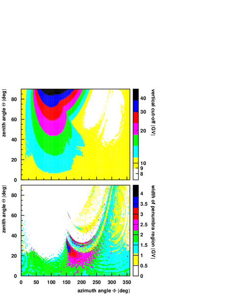
Figure 3: The mean geomagnetic cut-off and the width of the penumbra region for Kamioka, Japan. The width of the penumbra region is defined by the rigidity difference of the lowest momentum of an antiproton escaping to outer space and the highest momentum of an antiproton being trapped. The counting of the azimuth angle $\phi$, here and in all further plots, follows the convention used by the Super-Kamiokande detector, $\phi$ = 0^∘ means looking to the South (the particle travels to the North), $\phi$ = 90^∘ to the East (the particle travels to the West), etc. The North direction here is defined as the geographical one. The angle between the geomagnetic and geographic North direction in Kamioka is -7.59^∘.

II.4 The simulation of the geomagnetic cut-off

The Earth’s magnetic field has nearly the shape of a dipole field. The field is strong enough to deflect charged primary particles on their way to the Earth’s surface. While near the geomagnetic poles particles with very low momenta can penetrate to the Earth’s surface, protons with up to 60 GeV, impinging horizontally near the geomagnetic equator are reflected back to space.

The calculation of the geomagnetic cut-off is done in a Monte Carlo simulation of the possible particle trajectories in the so-called back-tracking method. Instead of tracking primary protons from outer space to the Earth’s surface, antiprotons from the surface are retraced to outer space. This method has the advantage that it allows to calculate in a straight forward way a table of allowed and forbidden trajectories. The entries in the table depend on the location on Earth, the arrival direction and the particle momentum.

In detail the particle tracking starts at 112.83 km, the top of atmosphere as defined in CORSIKA. The influence of the local magnetic field in the atmosphere, including the deflection of charged shower particles is handled lateron by CORSIKA using the approximation of a homogenous field.

The particle tracking is based on GEANT 3.21 gea (1993) and the magnetic field is described by the International Geomagnetic Reference Field IAGA Division V, Working Group 8, AOS (1992) for the year 2000. For the downward going particle fluxes the location where the primary particle enters the atmosphere is bound to the nearer surrounding of the experiment and the arrival direction is sampled in cells of a solid angle of 250 $\mu$sr. For upward going neutrinos the geomagnetic cut-off is calculated for 1655 locations, distributed nearly equidistant over the Earth’s surface, and the angle of incidence for each location is sampled in cells of 48 msr.

Instead of calculating a sharp cut-off, functions in momentum steps of 0.2 GeV/c up to a maximum momentum of 64 GeV/c are evaluated. This procedure accounts for the penumbra region of the cut-off, i.e. the chaotic change from open and closed trajectories which can be observed in irregular magnetic fields, as in case of the geomagnetic field.

As an example for the results obtained for a fixed detector location, the mean geomagnetic cut-off for particles entering the atmosphere in Kamioka is shown in Fig. 3. Local irregularities of the magnetic field over Japan cause a remarkable strong deviation from the regular shape expected for a magnetic dipole field. Assuming highly accurate Monte Carlo simulations and highly accurate measurements, this feature should be reflected in the zenithal and azimuthal dependence of the particle intensities in Kamioka.

Kamioka has a very extended penumbra region which exceeds a width of 4 GV in some particular directions. Details about the simulation of the geomagnetic cut-off and plots for other locations on the Earth may be found in Ref. Wentz et al. (2001b).

A check of the primary particle generator in CORSIKA with its assumptions for the solar modulation and the geomagnetic cut-off can be done by the recent results of the AMS-prototype mission Alcaraz et al. (2000c). Due to the inclination of 51.7^∘ of the shuttle orbit, the space craft passes geomagnetic latitudes from 0 to more than 1 rad.

The experimental spectra of downward going protons and helium nuclei can be compared rather directly with the results of the primary particle generator. Only a correction for the altitude dependence of the geomagnetic cut-off has to be applied. The cut-off has generally the highest value at the surface of the Earth, decreases with the altitude and vanishes when leaving the Earth’s magnetosphere. The mean difference in the cut-off between the top of atmosphere as assumed in CORSIKA and the orbit of the space shuttle is evaluated by a dedicated GEANT simulation and has a value of about 10 %.

Figure 4: Comparison of the AMS-results on downward going primary protons for different intervals of the geomagnetic latitude with spectra produced by the primary particle generator of CORSIKA including the simulation of the geomagnetic cut-off and the parametrization for the solar modulation.

The spectra of primary protons for different regions of the geomagnetic latitude together with the spectra produced by the primary particle generator of CORSIKA are shown in Fig. 4. The agreement between experiment and simulation is very good and the systematic decrease of the geomagnetic cut-off with the geomagnetic latitude is reproduced nicely. Only the spectrum for geomagnetic latitudes $0.9<\theta_{mag}<1$ shows a noticeable difference, which has to be attributed to the low absolute value of the cut-off which becomes comparable to the momentum steps used in the simulation of the cut-off functions. This disagreement has no significance for the calculation of atmospheric muon or neutrino fluxes, because the primary energies are already near or below the pion production threshold. The results obtained for primary helium nuclei have a similar quality.

Particles stored for longer times in the geomagnetic field, the so-called albedo or sub-threshold particles are not considered in the present calculations. It has been demonstrated in Ref. Lipari (2002) that they contribute to the atmospheric particle flux only negligibly.

II.5 The geography of the Earth in CORSIKA

The geography of the Earth plays a certain role in the simulation of atmospheric particle fluxes, because the apparent thickness of the atmosphere is altered by the different elevation of the terrain over sea-level and various climatic conditions on the density structure of the atmosphere. Also the local geomagnetic field, bending charged secondary particles in the atmosphere has quite a different strength for locations near the geomagnetic poles and the equatorial regions. For the geomagnetic poles the absolute field is found to be 64.6 $\mu$T, while the strength at the geomagnetic equator is only 21.7 $\mu$T.

Due to the vicinity of the place where the primary particle enters the atmosphere and the place of detection in the simulation of vertical downward going neutrinos, the geographic data are assumed as constant in the corresponding calculations. For the simulation of inclined particles, the distance in the locations may reach already 1200 km, and in case of upward going neutrinos the origin of the primary cosmic particles is distributed over the entire Earth.

Figure 5: The density distribution for atmospheric conditions of different climatic zones and seasons, plotted as mass overlay for a given altitude. In order to enhance the differences, the mass overlay for the altitude $h$ is multiplied by $\exp(h/8\,{\rm km})$. The differences for altitudes between 20 and 80 km are most important for atmospheric particle fluxes, while the differences over 80 km are artificially introduced by constraining all models to have zero density at 112.83 km (the starting altitude of CORSIKA). For the air shower development this is negligible, because the mass overlay at 80 km amounts to less than $10^{-2}$ g/cm².

Therefore, the local geomagnetic field is tabulated on basis of the International Geomagnetic Reference Field IAGA Division V, Working Group 8, AOS (1992) by a table containing the field parameters for 64800 locations distributed over the Earth’s surface. The elevation over sea-level is described in a table of equivalent resolution of data published by the US National Geophysical Data Center in Ref. National Geophysical Data Center (1988).

The atmospheric profiles observed in tropical and polar regions show considerable differences. The non-tropic atmospheres are subject to additional variations with the annual seasons. The extended CORSIKA code accounts for these effects by 7 atmospheric models  Kneizys et al. (1996). The corresponding density distributions are plotted in Fig. 5. As expected, the largest differences appear between the polar winter and summer. The seasonal variations become less important and vanish as the climatic zone approaches the equator.

II.6 The settings and the way of simulation in CORSIKA

The simulations discussed in this paper have been made using the CORSIKA program in version 6.000. All bugs found in CORSIKA until version 6.014 have been corrected also in the extended version.

The simulation of atmospheric particle fluxes with CORSIKA starts by selecting the type of primary particles and the ranges for the primary energy, zenith and azimuth angles, and by fixing the geographical location on Earth. The primary energies vary for all simulations reported in this paper between the minimum geomagnetic cut-off and $10^{15}$ eV.

The standard CORSIKA version makes use of a planar atmospheric model. This is a good approximation as long the zenith angle $\theta$ of the particles does not exceed 70^∘. The planar atmosphere approximation is used in this paper for the calculation of vertical muon fluxes, because the experiments are usually limited to muons having zenith angles less than 30^∘.

For the simulation of the East-West-effect of atmospheric muons and for all simulations of atmospheric neutrinos the zenith angles must be varied over the complete range. These simulations have been made with the so-called “curved” version of CORSIKA. Here the curvature of the Earth’s atmosphere is approximated by sliding and tilting plane atmospheres. Each time the horizontal displacement of a particle exceeds a limit of 6 to 20 km (dependent on the altitude), a transition to a new local plane atmosphere is performed Heck et al. (1999).

The different primary particles, i.e. protons and helium nuclei are simulated in separate runs and the ratio between them follows the absolute fluxes reported by the AMS prototype mission. In order to account for heavier primary particles the equivalent number of primary helium nuclei is used. The absolute fluxes of heavier nuclei are taken from the compilation of Wiebel-Sooth et al. Wiebel-Sooth et al. (1998). A justification of this simplification is provided by the fact that all heavier particles contribute together less than 5 % to the neutrino flux and all nuclei have a similar ratio of protons to neutrons.

The air shower calculation starts by getting a random location on the Earth, a random energy and a random arrival direction. If the particle does not exceed the geomagnetic cut-off for the given location or the solar modulation, a new set of geographic coordinates, energy and arrival angles is used. If the particle fulfills the requirements, the geomagnetic parameters, the altitude, and the atmosphere, are set according to the geographical position. Due to the long measuring time of Super-Kamiokande, atmospheric models for summer and winter are used in equal parts.

The primary particle is tracked to the first interaction point, given by the cross-section of the particle with air. The nuclear reaction is handled by the selected hadronic interaction model and all secondary particles are tracked up to their decay or further interactions.

The obtained numbers of atmospheric particles have to be normalized to the fluxes of primary particles. For sake of simplicity the number of primary particles with an energy larger than 1000 GeV in the simulation, being free of any influence of the geomagnetic cut-off and the solar modulation, is set equal to the integral flux above 1000 GeV as extrapolated in Sec. II.2. In cases with a limited statistical accuracy the calibration is made at 100 GeV. The fluxes at this energy are already influenced by the solar modulation by some 4.5 %, what has to be taken into account.

Due to the flat or partially flat geometry applied in CORSIKA, the obtained neutrino fluxes have to be scaled by the surface difference of the two shells having the radius of the Earth and the radius of the Earth plus 112.83 km. This correction leads to a factor of 1.036.

III Calculation of atmospheric muon fluxes

III.1 The differential muon flux

The calculation of atmospheric muon fluxes controls the calculations of atmospheric neutrino fluxes. The charge ratio of muons provides additional and partly complementary information.

Atmospheric muons have been measured over several decades. The data are compiled in two recent papers Vulpescu et al. (1998); Hebbeker and Timmermans (2002) and in the new review Grieder (2001), showing relatively large discrepancies between the experiments. The comparisons of this communication are focused on the recent measurements of BESS, CAPRICE, the OKAYAMA cosmic ray telescope and WILLI. In case of BESS Motoki et al. (2001, 2002) and CAPRICE Kremer et al. (1999) the results of atmospheric muons have been obtained in ground based runs, performed as test of the detectors. The OKAYAMA telescope Tsuji et al. (1998) is a classical magnetic spectrometer and WILLI Vulpescu et al. (1998, 2001) represents a compact scintillator experiment dedicated to the precise measurement of the muon charge ratio. The charge ratio is deduced hereby from the different life time of positive and negative muons in matter.

Table 2: The geographical parameters for the different detector sites. The quantity $h$ is the elevation over sea-level, $R_{c}$ the mean vertical geomagnetic cut-off, $B_{x}$ the horizontal component of the magnetic field, $B_{z}$ the vertical downward component and $B_{\alpha}$ is the angle between the magnetic and geographic north direction. The parameters of the magnetic field are valid for the year 2000 and an altitude of 56.4 km.

site	$h$ [m]	$R_{c}$ [GV]	$B_{x}$ [$\mu$T]	$B_{z}$ [$\mu$T]	$B_{\alpha}$ [deg]
Bucharest	85.	5.6	21.98	40.96	3.64
Fort Sumner	1270.	4.2	22.89	44.33	9.44
Lynn Lake	360.	0.5	9.81	57.51	9.36
Okayama	5.3	11.8	30.48	34.31	-6.64
Tsukuba	30.	11.5	29.08	34.82	-6.95

For the simulation of the atmospheric muon fluxes the precise geographical parameters, like the geomagnetic cut-off and the altitude of the different detector sites are taken into account. The used parameters are compiled in Tab. 2. Due to the geographic vicinity of Okayama and Tsukuba and the same altitude of both sites, the results of the OKAYAMA telescope can be compared directly with the measurements and calculations done for Tsukuba.

Figure 6: The differential flux of vertical muons calculated by CORSIKA using different models for the description of the hadronic interaction in comparison with experimental results for various detector sites. In order to enhance the differences in the region of interest, the fluxes are multiplied with the muon momentum $p_{\mu}$.

The results for the differential flux of vertical muons are compiled in Fig. 6. The calculation with DPMJET as well as the calculations with VENUS + UrQMD agree generally well with the experimental data. Only the GHEISHA results show a strange enhancement of the differential muon flux for low energies and quite a different momentum dependence.

III.2 The charge ratio of muons

In contrast to the differential muon fluxes, the charge ratio of muons reveals larger discrepancies. The CORSIKA results for the charge ratio of muons are compared in Fig. 7 with the experimental data. Again the results obtained with the GHEISHA model are far from the experimental observations but there are also differences between the results of DPMJET and VENUS + UrQMD. The results obtained with VENUS + UrQMD are lower than the experimental values especially for low and intermediate energies. It has been shown, that this deviation originates mainly from UrQMD while at higher energies VENUS leads to a muon charge ratio which is compatible to the measurements Wentz et al. (2001c).

Figure 7: The charge ratio of muons calculated by CORSIKA using different models for the description of the hadronic interaction compared to experimental data from various detectors.

The DPMJET results agree generally well with the data, with exception of the CAPRICE results in Fort Sumner. The deviation for Fort Sumner has to be questioned because the geomagnetic cut-off in Fort Sumner resembles that in Bucharest. Therefore the differences in the experimental values and the continuous increase of the charge ratio in the CAPRICE measurement for Fort Sumner far beyond the geomagnetic cut-off seem to indicate experimental problems in this particular measurement.

The real influence of the geomagnetic cut-off on the muon charge ratio can be seen when comparing the CAPRICE and BESS results for Lynn Lake, the WILLI results for Bucharest, and the BESS results for Tsukuba. At higher energies the ratio stays nearly constant, however it decreases, when the geomagnetic cut-off clips the high excess of low energy primary protons, as can be observed in the results for Bucharest and Tsukuba. This effect is nicely reproduced by CORSIKA using DPMJET as interaction model, while using UrQMD the effect is covered by intrinsic problems of the model.

The systematics of the geomagnetic cut-off shows again the problem of the CAPRICE results for Fort Sumner. The CAPRICE results have practically the same dependence on the momentum as the BESS results in Tsukuba, where the geomagnetic cut-off is nearly 3 times higher.

It could be argued that Fort Sumner has an altitude of 1230 m above sea level and there could be a strong dependence of the charge ratio on the altitude, but the CORSIKA simulations include the precise altitude and the recent results from BESS show only a weak dependence of the charge ratio on the altitude. The BESS data indicate a 3 % difference between Tsukuba and Mt. Norikura which has an altitude of 2770 m Sanuki et al. (2002).

The disability of GHEISHA, the standard hadronic interaction model in the detector simulation tool GEANT 3.21, in reproducing the data of atmospheric muons surprises. But in fact serious deficits of GHEISHA have already been proved in direct model tests. In Refs. Ferrari and Sala (1996); Wentz et al. (1999, 2001c) it has been reported that GHEISHA violates the energy, momentum, charge and baryon number conservation in the single hadronic interaction.

At least the energy conservation is also violated on average as can be shown by the simulation of extensive air showers with standard CORSIKA. CORSIKA allows to summarize all the energy deposited in the atmosphere during the shower development. Using GHEISHA as low energy hadronic interaction model, an augmentation of energy of a complete shower is observed. This increase of energy is about 5 % at 10¹⁵ eV and 7 % at 10¹⁴ eV. Therefore, the GHEISHA version used in GEANT3 gea (1993) should not be used in any serious simulation of atmospheric neutrino fluxes. This holds especially for the neutrino flux calculations of Plyaskin, which are based on GHEISHA, only. After finishing the simulations, correction patches for GHEISHA became available which improve essentially the energy conservation Cassell and Bower (2002).

Figure 8: The East-West-effect of the muon charge ratio as measured by the WILLI detector in comparison with calculations of CORSIKA using DPMJET. The detector acceptance of WILLI is taken into account by processing the raw results of CORSIKA by the detector simulation program of WILLI. East and WEST mean that the detector looks to the East and West, respectively.

III.3 The East-West-effect of the muon charge ratio

Data for inclined muons allow a check of the calculations in the curved geometry of the Earth. Using the so-called East-West-effect of the muon charge ratio, caused by the influence of the geomagnetic field, the way of handling the field in the calculation can be verified, too.

Fig. 8 shows preliminary results of the WILLI experiment for muons observed in East and West direction having a mean zenith angle of 35^∘ Brancus et al. (2002) in comparison with CORSIKA simulations on basis of DPMJET. The CORSIKA results are processed by a full detector simulation of the experiment in order to account for the complex acceptance of the instrument.

The agreement of the CORSIKA results with the strong East-West-effect observed by the WILLI experiment, gives confidence that the corresponding effect in the atmospheric neutrino flux is also handled well by CORSIKA.

Muon data in various depths of the atmosphere would provide a further possibility for the revision of calculations on atmospheric particle fluxes. Unfortunately the rise and decline time of the actual balloon measurements are such fast, that the corresponding muon data have large statistical errors. Additionally the atmospheric pion flux causes systematic errors in some instruments. While the pion flux on sea-level is only 0.5 % of the muon flux it reaches 50 % when approaching the top of atmosphere.

Nevertheless it has to be pointed out that the atmospheric muon flux, in contrast to the neutrino flux where every produced neutrino reaches ground level, is a highly differential quantity, because most muons are already absorbed before reaching ground level. Therefore possible differences, for example in the nuclear interaction models are enhanced from one hadronic interaction to the next. Thus the calculation of the ground level muon flux has higher theoretical uncertainties than the calculation of atmospheric neutrino fluxes.

IV Calculation of atmospheric neutrino fluxes

IV.1 The vertical neutrino fluxes in Kamioka

The calculation of atmospheric neutrino fluxes for Kamioka is split in two separate calculations. The downward going neutrinos are simulated locally for Kamioka, while the upward going neutrinos are calculated from primary particles distributed over the entire Earth and only neutrinos passing in a circle of 1000 km distance from Kamioka are used in the further analysis.

Figure 9: The vertical differential intensities of the different neutrino flavors in Kamioka, displayed as the ratio between the CORSIKA results using DPMJET as hadronic interaction model and the calculations of BGS, HKHM and BFLMSR.

Table 3: The vertical differential intensity $f(\nu)$ and the errors $\Delta(\nu)$ for downward going neutrinos in Kamioka as calculated with CORSIKA using DPMJET and VENUS + UrQMD. The fluxes and the corresponding statistical errors due to the limited number of events in the Monte Carlo simulation are given in units of (m² s sr GeV)^-1.

	DPMJET								VENUS + UrQMD
$E_{\nu}$ $[$GeV$]$	$f(\nu_{e})$	$\Delta(\nu_{e})$	$f(\overline{\nu_{e}})$	$\Delta(\overline{\nu_{e}})$	$f(\nu_{\mu})$	$\Delta(\nu_{\mu})$	$f(\overline{\nu_{\mu}})$	$\Delta(\overline{\nu_{\mu}})$	$f(\nu_{e})$	$\Delta(\nu_{e})$	$f(\overline{\nu_{e}})$	$\Delta(\overline{\nu_{e}})$	$f(\nu_{\mu})$	$\Delta(\nu_{\mu})$	$f(\overline{\nu_{\mu}})$	$\Delta(\overline{\nu_{\mu}})$
0.112	1303.	6.1	1251.	5.9	2708.	8.8	2727.	8.8	1341.	6.4	1330.	6.4	2838.	9.3	2857.	9.4
0.141	1142.	5.1	1100.	5.0	2336.	7.2	2329.	7.2	1154.	5.3	1153.	5.3	2430.	7.7	2422.	7.7
0.178	921.3	4.1	875.5	4.0	1894.	5.8	1870.	5.8	932.5	4.2	920.7	4.2	1995.	6.2	1985.	6.2
0.224	702.1	3.2	655.1	3.0	1455.	4.5	1432.	4.5	703.0	3.3	678.3	3.2	1526.	4.8	1506.	4.8
0.282	506.0	2.4	473.3	2.3	1075.	3.5	1050.	3.4	505.0	2.5	488.5	2.4	1114.	3.7	1094.	3.7
0.355	361.6	1.8	327.8	1.7	775.8	2.6	755.8	2.6	347.6	1.8	334.3	1.8	776.9	2.7	769.5	2.7
0.447	247.8	1.3	221.3	1.3	542.1	2.0	526.3	1.9	231.4	1.3	218.1	1.3	528.1	2.0	512.7	2.0
0.562	164.1	.96	142.9	.90	371.7	1.4	358.8	1.4	150.8	.96	140.0	.93	349.6	1.5	340.3	1.4
0.708	106.8	.69	92.10	.64	246.3	1.1	234.3	1.0	94.37	.68	85.94	.65	224.2	1.0	212.4	1.0
0.891	66.74	.49	56.19	.45	160.2	.76	149.0	.73	57.09	.47	50.84	.44	140.4	.74	134.1	.72
1.122	39.37	.33	33.05	.31	99.78	.53	92.37	.51	32.49	.32	29.51	.30	84.70	.51	80.70	.50
1.413	23.33	.23	19.20	.21	59.89	.37	54.97	.35	18.74	.21	16.47	.20	50.29	.35	46.93	.34
1.778	12.89	.15	10.22	.14	33.97	.25	30.76	.23	10.21	.14	8.636	.13	28.59	.24	26.40	.23
2.239	6.746	.098	5.366	.087	19.23	.17	16.50	.15	5.345	.091	4.579	.084	15.73	.16	14.30	.15
2.818	3.413	.062	2.632	.054	10.24	.11	8.821	.10	2.609	.056	2.270	.053	8.783	.10	7.615	.096
3.548	1.611	.038	1.347	.035	5.236	.068	4.432	.063	1.258	.035	1.115	.033	4.645	.067	3.983	.062
4.467	.741	.023	.583	.020	2.566	.043	2.168	.039	.6162	.022	.5615	.021	2.490	.044	2.106	.040
5.623	.299	.013	.241	.012	1.266	.027	1.044	.024	.3047	.014	.2447	.012	1.269	.028	1.065	.026
7.079	.133	.0077	.117	.0073	.6337	.017	.4648	.014	.1278	.0079	.0991	.0069	.5997	.017	.5384	.016
8.913	.060	.0046	.049	.0042	.2966	.010	.2328	.0091	.0749	.0054	.0452	.0042	.3104	.011	.2320	.0095
11.22	.023	.0026	.016	.0022	.1504	.0065	.1210	.0059	.02913	.0030	.0187	.0024	.1674	.0072	.1168	.0060

Figure 10: The vertical differential intensities of the different neutrino flavors in Kamioka. Shown is the ratio between the CORSIKA results using VENUS + UrQMD as hadronic interaction model and the calculations of BGS, HKHM and BFLMSR.

This procedure causes a large difference in the number of primary particles needed in the simulation for obtaining the same statistical accuracy for the up- and downward going fluxes. In the present simulation the number of upward going neutrinos is still a factor of 8 smaller.

Tab. 3 gives the differential intensities for vertical neutrinos obtained with CORSIKA, using DPMJET and VENUS + UrQMD, respectively. In Figs. 9 and 10 the results are compared directly with the calculations of BGS, HKHM and BFLMSR.

The inclusive neutrino fluxes obtained with CORSIKA are evidently lower than the fluxes given by BGS and HKHM. The differential fluxes at 0.1 GeV are about 40 % smaller than the BGS fluxes and become comparable at energies in the GeV range. The agreement of the CORSIKA results using DPMJET and using VENUS + UrQMD with the BFLMSR calculation is better. The deviation of these absolute flux calculations over practically the whole energy range remains less than 20 %. The energy dependence of the neutrino fluxes between BFLMSR and VENUS + UrQMD is quite similar while DPMJET shows a systematic difference to BFLMSR.

Fig. 11 displays the ratio between the different neutrino flavors in the vertical downward going flux. The agreement of all calculations for the ratio of muon neutrinos to electron neutrinos is very good. The deviation of the HKHM results and the discontinuity at $E_{\nu}\,=\,1$ GeV are caused by different approaches in the model. Below 1 GeV the values of HKHM are averaged over the zenith angle, only above 1 GeV they stand for vertical, downward going neutrinos. For energies below 3 GeV the differences between the other models are on the level of 2 % or better.

Some differences between the calculations are observed in the ratio of muon neutrinos to muon antineutrinos. The CORSIKA calculations with DPMJET and VENUS + UrQMD, and the BFLMSR calculations agree perfectly. The calculations of BGS predict a lower ratio at 3 GeV while the calculations of HKHM are different around 1 GeV and show a smaller rise of the ratio at high energies.

The ratio of electron neutrinos to electron antineutrinos reveals larger differences. The results of HKHM behave quite different from the results of all other models. Interestingly, DPMJET results agree with BFLMSR results, while VENUS + UrQMD results agree with BGS results. Due to the close correlation between the ratio of electron neutrinos to electron antineutrinos and the charge ratio of muons, these findings allow to rule out the results of VENUS + UrQMD in this particular quantity, meaning that the results of BGS are suspicious in this aspect, too.

Figure 11: The ratio between different neutrino flavors in the vertical flux in Kamioka as calculated by CORSIKA with DPMJET and with VENUS + UrQMD.

An interesting quest for the CORSIKA calculations with their inclusion of the precise geometry of the Earth, are natural differences between the up- and downward going neutrino fluxes in Kamioka. Such differences could contribute to the measured asymmetry, which is commonly attributed to the oscillation of neutrinos. Any natural difference based on the geographical environment has a direct impact on the analysis of the neutrino oscillations and changes finally the obtained oscillation parameters.

Figure 12: The asymmetry of the up- ($N_{u}$) and downward ($N_{d}$) going neutrino fluxes for Kamioka as calculated by CORSIKA using DPMJET and VENUS + UrQMD in comparison with the calculation of BFLMSR. The asymmetry is expressed by the ratio between the difference and the sum of the up- and downward going neutrino fluxes.

A major difference between Kamioka and its antipode in the South Atlantic comes from the geomagnetic cut-off. While the vertical cut-off in Kamioka is 12.3 GV, the South Atlantic region is influenced by the so-called South Atlantic magnetic field anomaly leading to a vertical cut-off at the antipode of only 8.6 GV. This causes an asymmetry between the intensities of up- and downward going neutrinos for Kamioka, as can be seen in Fig. 12.

The asymmetry of 20 % having been observed in the calculations of BFLMSR represents the raw effect based on the differences in the geomagnetic cut-off, because the calculation does not include any local magnetic field. In the CORSIKA simulations the local field and an additional contribution to the up-down asymmetry, caused by the different elevation of the surface over sea-level in Kamioka and in the antipode region in the South Atlantic, are taken into account.

Figure 13: The zenith angle dependence of the neutrino intensities in Kamioka as calculated by CORSIKA with DPMJET and with VENUS + UrQMD in comparison with the calculations of BFLMSR and BGS. The first column shows the plots for the energy interval 0.1 to 0.31 GeV, the second for 0.31 to 1 GeV, the third for 1 to 3.1 GeV, and the last for 3.1 to 10 GeV.

The location of the Super-Kamiokande detector in the mountains causes an altitude difference of several hundred meters compared to the average altitude of the antipode region. Thus in the South Atlantic the shower development is longer and more neutrinos are produced in the shower. Further details on the influence of the local magnetic field and the geomagnetic cut-off are investigated in Sec. IV.3. The effect of the contrary seasons in Japan and the South Atlantic, which is taken into account by using the appropriate atmospheric models does not lead to any observable effect, the effect is smaller than the actual statistical errors.

Figure 14: The results of CORSIKA using DPMJET and VENUS + UrQMD for the zenith angle dependence of the different ratios between the neutrino flavors. The values are compared with the calculations of BFLMSR and BGS. The plots in the first row are for the energy interval 0.1 to 0.31 GeV and in the second row for 0.31 to 1 GeV. If the error bar is not drawn, the error is smaller than the symbol size.

Figure 15: The azimuth angle dependence of the neutrino fluxes in Kamioka as calculated with CORSIKA for different energies and neutrino flavors compared with the calculations of HKKM. The data in the first row are integrated in an energy interval from 0.1 to 0.3 GeV, in the second row from 0.3 to 1 GeV, and in the third row from 1 to 3.1 GeV. The neutrinos selected are from both hemispheres and have a $|\cos\theta|>0.5$. In this diagram $\phi=0$ indicates a particle going in the magnetic North direction. The errors are smaller than the symbol sizes.

IV.2 The directional dependence of the neutrino fluxes in Kamioka

The dependence of the neutrino fluxes on the zenith angle is shown in Fig. 13. The three dimensional calculations of BFLMSR and CORSIKA show an enhancement of the neutrino fluxes near the horizon. This enhancement is based on a geometrical effect, i.e. the spherical shell geometry of the neutrino production volume Lipari (2000). This effect has been neglected in all one dimensional simulations like HKHM and BGS. The strength of the effect shows clearly the necessity of the time consuming three dimensional simulations in a spherical geometry. The agreement of the calculation with VENUS + UrQMD and with BFLMSR is again better, while the DPMJET results show systematically higher fluxes for energies between 1 and 3 GeV.

The dependence of the resulting ratio between muon neutrinos and electron neutrinos on the zenith angle is shown in Fig. 14. Only the results for energies below 1 GeV are plotted, for higher energies no difference between all the four calculations is observed. As in the case of the ratios between vertical neutrino fluxes the largest differences are observed in the ratio of electron neutrinos to electron antineutrinos. The CORSIKA results show a strong increase of the ratio near the horizon. The origin of this effect will be investigated in Sec. IV.3.

Also a 8 % difference of the ratio of muon neutrinos to electron neutrinos at low energies can be observed near the horizon. The results of the BGS calculation lead to very low values for this quantity, and may be an artifact of the calculation in a one dimensional geometry.

The dependence of the neutrino fluxes on the azimuth angle is shown in Fig. 15. The agreement between the calculations with DPMJET and with VENUS + UrQMD for westward going neutrinos is very good, but for eastward going neutrinos some noticeable differences are observed at higher energies. This is a secondary effect of the difference in the momentum spectra of the reaction products between both models, but it displays also an instructive example how the interaction model influences results which are commonly assumed to have a geometrical nature.

The detailed comparison with the results of the HKKM calculation shows a very good agreement in the shape of the azimuthal distribution. At lowest energies the HKKM calculation leads to much higher fluxes. The authors state this overestimation to be caused by the use of the old COSMOS interaction models. A new calculation using DPMJET as hadronic interaction model will overcome this problem.

Figure 16: The azimuth angle dependence of the neutrino fluxes as calculated by CORSIKA with DPMJET and with VENUS + UrQMD, compared with a calculation of Lipari et al. Lipari et al. (1998); Lipari (2000). The neutrinos used in the analysis result from both hemispheres, requesting $|\cos\theta|>0.5$ and an energy between 0.5 and 3 GeV. The calculations of Lipari have been normalized to the fluxes obtained with DPMJET. In this diagram $\phi=0$ indicates a particle going towards the magnetic North direction. The errors are smaller than the symbol sizes.

The good agreement between CORSIKA results and the calculation of HKKM in the azimuthal distribution is by far not trivial, as shows the comparison of the CORSIKA results with calculations of Lipari et al. Lipari et al. (1998); Lipari (2000) in Fig. 16. Here the shapes of the distributions for electron neutrinos and muon antineutrinos are compatible, but strong disagreement exists for electron antineutrinos and muon neutrinos.

Figure 17: The energy dependence of the East-West-asymmetry in the atmospheric neutrino flux as calculated by CORSIKA with DPMJET and with VENUS + UrQMD.

Figure 18: Zenith angle dependence of the ratio between electron neutrino and electron antineutrino fluxes in Kamioka. The results of CORSIKA with DPMJET considering the local magnetic field are compared with results of CORSIKA and BFLMSR neglecting the local magnetic field.

The results can be expressed by the East-West-asymmetry $A_{EW}=(N_{E}-N_{W})/(N_{E}+N_{W})$, where $N_{E}$ and $N_{W}$ stand for the particle fluxes of neutrinos going to the East and West, respectively. Fig. 17 shows the energy dependence of the East-West-asymmetry. Again the CORSIKA results with DPMJET have a slightly higher asymmetry than the calculations with VENUS + UrQMD. The distributions of all neutrino flavors show similar shapes. The strongest asymmetry is observed for electron neutrinos and the weakest for electron antineutrinos. All neutrino flavors exhibit a maximal asymmetry for an energy around 800 MeV.

Figure 19: The azimuth angle dependence of the atmospheric neutrino fluxes in Kamioka as calculated by CORSIKA under different conditions. The neutrinos used in the analysis result from both hemispheres and have a $|\cos\theta|>0.5$. Beside the results described already above, the azimuthal distributions are shown for a zero local magnetic field, a zero geomagnetic cut-off and an isotropic cut-off of 6 GV. In this diagram $\phi=0$ indicates a particle going towards the magnetic North direction. The distributions in the first row are integrated over an energy interval between 0.1 and 0.3 GeV, in the second between 0.3 and 1 GeV, and in the third between 1 and 3.1 GeV.

IV.3 The influences of the geomagnetic cut-off and the local magnetic field

In order to investigate the individual influences of the geomagnetic cut-off and of the local magnetic field, the calculations of the atmospheric neutrino fluxes for Kamioka with DPMJET have been repeated twice under the same conditions, except setting once the local magnetic field and once the geomagnetic cut-off to zero. This procedure allows to disentangle the individual influences of the two effects.

Due to the fact that charged particles do not win or loose energy in a magnetic field, the influence of the local magnetic field on the total neutrino fluxes is negligible. The main effects are expected in the ratios of neutrinos and in the azimuthal distribution of the fluxes. Especially the ratio of electron neutrinos to electron antineutrinos shows a strong effect because the electron neutrinos are predominantly produced by positive muons and the electron antineutrinos by negative muons.

Muon neutrinos and muon antineutrinos are produced also in the decay of charged pions. In contrast to the muon decay, muon neutrinos result here from the decay of positive and muon antineutrinos from the decay of negative particles. Due to the shorter life time and the higher momentum the total bending of pions is less and the bending of the muons is preponderating, but the total effect of the local magnetic field on the muon neutrinos remains weaker.

The effect of the inclusion of the local magnetic field in the calculation is shown in Fig. 18. The increase of the ratio between electron neutrinos and electron antineutrinos near the horizon as observed in Fig. 14 has to be attributed completely to the bending of the charged shower particles in the atmosphere.

The CORSIKA results for the azimuthal dependence of the atmospheric neutrino fluxes under the different conditions are displayed in Fig. 19. The differences are pronounced for smaller energies. At higher energies all the different conditions lead to identical fluxes. The influence on the shape of the azimuthal distribution is weak, but only for detector sites with a high geomagnetic cut-off.

Without consideration of the geomagnetic cut-off, much higher neutrino fluxes are obtained due to the higher fluxes of primary particles. The asymmetry in the azimuthal distribution results here only from the deflection of charged shower particles in the local magnetic field. The characteristics of this asymmetry is very similar to the East-West-effect caused by the geomagnetic cut-off, a consequence of the excess of positive particles in the atmosphere, on which the magnetic field acts in a similar way as on the primary proton flux. This argument is supported by the different behavior of electron antineutrinos, which are produced only in the decay of negative muons.

In order to illustrate the transition between a zero and a high geomagnetic cut-off, the results of a calculation assuming an isotropic cut-off of 6 GV have been added also in Fig. 19. These results show that a neglect of the local magnetic field, as it is done in many calculations of atmospheric neutrino fluxes, may lead to wrong azimuthal distributions at least for detector sites with a comparable low geomagnetic cut-off.

V Conclusion

This work aims at a new procedure for the calculation of atmospheric neutrino fluxes with considering various influences which have not been taken into account so far or, if ever, only in a less rigorous way. The capabilities of the procedure are demonstrated by a particular calculation of the detailed neutrino fluxes in Kamioka. The detailed procedure applies the air shower simulation code CORSIKA in the version 6.000, which has been extended and modified for a reliable simulation of the cascading interactions induced in the atmosphere by primary particles of the low energy part of the cosmic ray spectrum.

A description of the solar modulation and tables for the geomagnetic cut-off, calculated in a detailed Monte Carlo simulation, have been introduced. In addition, for the first time for atmospheric neutrino flux calculations, the geography of the Earth is taken into account by a digital elevation model, tables for the local magnetic field in the atmosphere, and various atmospheric models for different climatic zones and seasons. These extensions are not yet part of the standard CORSIKA package.

CORSIKA features a precise particle tracking, including the deflection of the charged shower particles in the local magnetic field, the energy loss by ionization and multiple scattering. The used primary flux is based on the recent measurements of the prototype of the AMS-experiment. These data allow also a test of the calculations for the geomagnetic cut-off.

An important aspect of the calculations is the question of the adequate hadronic interaction model used as generator of the flux calculations. This question is approached by using the possibilities of the CORSIKA code to operate optionally with various different hadronic interaction models. The models are scrutinized by an extensive comparison with measured fluxes and charge ratios of atmospheric muons in different locations.

It turns out that the GHEISHA model leads to significant discrepancies with data from various experiments and predictions based on GHEISHA have to be considered as highly doubtful. The use of DPMJET II.5 as well as of the combination VENUS + UrQMD results in differential muon fluxes which are in good agreement with the measurements. The DPMJET model reproduces the charge ratio of muons of vertical incidence, while the values obtained with VENUS + UrQMD appear systematically too small. The calculations with DPMJET agree also well with the preliminary results of the WILLI experiment for the East-West-effect of the charge ratio of muons with inclined incidence.

Subsequently CORSIKA is used with the described refinements to calculate the fluxes of atmospheric neutrinos for Kamioka. The resulting absolute neutrino intensities are lower than those found in the classical calculations of BGS and HKHM, but they are in good agreement with the recent three dimensional calculations of BFLMSR. Using VENUS + UrQMD the deviations from BFLMSR predictions are smaller than 20 % over the whole energy range and the overall energy dependence is very similar.

DPMJET leads to absolute fluxes, being also very similar to the simulations of BFLMSR, but the energy dependence turns out to be slightly different. Nevertheless the better agreement of the DPMJET predictions with the measured fluxes and charge ratios of atmospheric muons provides stringent arguments in favor of this particular model.

The ratio of muon neutrinos to electron neutrinos and the ratio of muon neutrinos to muon antineutrinos in the vertical downward flux are identical within the statistical uncertainties for the CORSIKA calculations invoking DPMJET, VENUS + UrQMD, and the calculations of BFLMSR. But for lowest energy neutrinos with horizontal incidence, the ratios between muon neutrinos and electron neutrinos obtained with DPMJET and with VENUS + UrQMD are higher.

Significant differences are observed for the ratio of electron neutrinos to electron antineutrinos. The DPMJET results for vertical neutrinos for this quantity agree with the results of BFLMSR, and the results of VENUS + UrQMD agree with the results of BGS. Again the very good agreement in the correlated quantity of the muon charge ratio gives a strong argument for DPMJET. For horizontal neutrinos the CORSIKA results predict a strong increase of the ratio at low energies.

The actual results have relevance for the analysis of the atmospheric neutrino anomaly. Any change in the ratio of muon neutrinos to electron neutrinos leads directly to a change of the oscillation parameters. Also the discrepancies found in the ratio of electron neutrinos to electron antineutrinos are of particular interest for Super-Kamiokande, because the detection cross-sections for neutrinos are about three times larger than for antineutrinos and it is not possible to distinguish between them in the experiment.

To quantify the influence of these effects on the neutrino oscillation parameters would request a full detector simulation of the Super-Kamiokande experiment based on the presented fluxes, a task which is beyond the scope of this communication. It can be stated that the difference of the neutrino fluxes presented here to those used in the oscillation analysis is not large enough to affect the claim of existence of neutrino oscillations from atmospheric neutrinos.

The use of two different hadronic interaction models, both of good repute in interpretation of accelerator experiments, shows clearly the potential influence of the hadronic interaction model on the interpretation of the atmospheric neutrino anomaly. Due to the high quality of the recent measurements of the primary particle fluxes, the main source of remaining uncertainties in the atmospheric flux calculations has to be attributed now to the actual uncertainties in the hadronic interaction models.

For studying the influence of the geomagnetic field and the origin of the East-West-effect in the atmospheric neutrino flux, CORSIKA calculations with DPMJET, setting the local magnetic field to zero or skipping the geomagnetic cut-off have been performed. The main influence of the local magnetic field is found for the ratio of electron neutrinos to electron antineutrinos. CORSIKA predicts for the first time a strong increase of the ratio near the horizon.

The local magnetic field proves to be of minor influence on the azimuthal distribution of neutrinos in Kamioka, and the East-West-effect arises mainly from the azimuthal dependence of the primary particle flux caused by the geomagnetic cut-off rigidity. The simulations without a geomagnetic cut-off show that this observation is valid only for Kamioka with its relative high geomagnetic cut-off value. For a neutrino detector site like Sudbury in Canada, where the vertical geomagnetic cut-off is only 1.1 GV, a measurable East-West-effect would originate exclusively from the bending of the charged shower particles in the local magnetic field.

To which extent the Earth’s geography significantly affects the results of the calculations has not been investigated in detail by separate calculations. The higher asymmetry of the up- and downward going particle fluxes, found in the actual calculations in comparison to results of BFLMSR, indicates an influence of the digital elevation model in the order of a few percent. Compared to the changes of the atmospheric depth by the different altitudes, the variation induced by the different atmospheric models is small. The influence on the particle fluxes in Kamioka should be negligible. Nevertheless for detector sites with extreme atmospheric conditions, like the South Pole, the profile of the atmosphere may lead to noticeable seasonal effects.