Multiple Parton Scattering in Nuclei: Beyond Helicity Amplitude Approximation

Abstract

Multiple parton scattering and induced parton energy loss in deeply inelastic scattering (DIS) off heavy nuclei is studied within the framework of generalized factorization in perturbative QCD with a complete calculation beyond the helicity amplitude (or soft bremsstrahlung) approximation. Such a calculation gives rise to new corrections to the modified quark fragmentation functions. The effective parton energy loss is found to be reduced by a factor of 5/6 from the result of helicity amplitude approximation.

I Introduction

Suppression of jet production or jet quenching in high-energy nuclear collisions has been proposed as a good probe of the hot and dense medium [1, 2] that is produced during the violent collisions. The quenching of an energetic parton is caused by multiple scattering and induced parton energy loss during its propagation through the hot QCD medium. It suppresses the final leading hadron distribution giving rise to modified fragmentation functions and the final hadron spectra [3, 4]. Recent theoretical estimates [5, 6, 7, 8, 9] all show that the effective parton energy loss is proportional to the gluon density of the medium. Therefore measurements of the parton energy loss will enable one to extract the initial gluon density of the produced hot medium. Strong suppression of high transverse momentum hadron spectra is indeed observed by experiments [10, 11] at the Relativistic Heavy-Ion Collider (RHIC) at the Brookhaven National Laboratory (BNL), indicating large parton energy loss in a medium with large initial gluon density. However, one cannot unambiguously extract the initial gluon density from the experiments of heavy-ion collisions alone because of the theoretical uncertainty in relating the parton energy loss to the initial gluon density. For this purpose, one has to rely on other complimentary experimental measurements such as parton energy loss in deeply inelastic scattering (DIS) of nuclear targets. One can then at least extract the initial gluon density in heavy-ion collisions relative to that in a cold nucleus [12].

Modified quark fragmentation function inside a nucleus in DIS and the effective parton energy loss has been derived recently by Guo and Wang [13]. Generalized factorization of twist-four processes [14] was applied to the inclusive process of jet fragmentation in DIS in order to derive the modified fragmentation functions. Taking into account of gluon bremsstrahlung induced by multiple parton scattering and the Landau-Pomeranchuck-Migdal (LPM) interference effect, one finds that the leading twist-four contributions to the modified fragmentation function and the effective parton energy loss depend quadratically on the nuclear size $R_{A}$. They also depend linearly on the effective gluon distribution in nuclei. One can also extend the study to parton propagation inside a hot QCD medium reproducing earlier results [12]. This allows one to relate parton energy loss in both hot and cold nuclear medium.

There are all together 23 cut-diagrams that contribute to the leading twist-four corrections to the quark fragmentation function in $eA$ DIS. For simplification of the calculation, the helicity amplitude approximation was used in Ref. [13] in the limit of soft gluon radiation $z_{g}=1-z\rightarrow 0$ where $z_{g}$ is the momentum fraction carried by the radiated gluon and $z$ the fraction carried by the leading quark. Such an approximation enables one to simplify the calculation of the radiation amplitudes. The final results are obtained by squaring the sum of all possible amplitudes, giving rise not only to the contributions of double scattering but also various interferences. In this approximation, the amplitudes of initial and final state radiation are the same except the opposite signs and different color matrices. Because of the different color matrices in the initial and final state radiation, there is no complete cancellation of the radiation amplitudes. In addition, there is also gluon radiation from the exchanged gluon via triple-gluon coupling. These non-Abelian features of QCD radiation lead to a finite gluon spectra even in the helicity amplitude approximation. However, under the same approximation, the photon spectra from QED bremsstrahlung would be zero because of almost complete cancellation between initial and final state radiation. One therefore has to go beyond the helicity approximation. In this paper, we will study the correction to the gluon radiation spectra when we go beyond the helicity amplitude approximation and its effect in the modified quark fragmentation function. We will also compute the effective quark energy loss and compare to the result in the helicity amplitude approximation.

II Generalized Factorization

In order to study the quark fragmentation in $eA$ DIS, we consider the following semi-inclusive processes, $e(L_{1})+A(p)\longrightarrow e(L_{2})+h(\ell_{h})+X$, where $L_{1}$ and $L_{2}$ are the four momenta of the incoming and the outgoing leptons, and $\ell_{h}$ is the observed hadron momentum. The differential cross section for the semi-inclusive process can be expressed as

$$E_{L_{2}}E_{\ell_{h}}\frac{d\sigma_{\rm DIS}^{h}}{d^{3}L_{2}d^{3}\ell_{h}}=\frac{\alpha^{2}_{\rm EM}}{2\pi s}\frac{1}{Q^{4}}L_{\mu\nu}E_{\ell_{h}}\frac{dW^{\mu\nu}}{d^{3}\ell_{h}}\;,$$ (1)

where $p=[p^{+},0,{\bf 0}_{\perp}]$ is the momentum per nucleon in the nucleus, $q=L_{2}-L_{1}=[-Q^{2}/2q^{-},q^{-},{\bf 0}_{\perp}]$ the momentum transfer, $s=(p+L_{1})^{2}$ and $\alpha_{\rm EM}$ is the electromagnetic (EM) coupling constant. The leptonic tensor is given by $L_{\mu\nu}=1/2\,{\rm Tr}(\gamma\cdot L_{1}\gamma_{\mu}\gamma\cdot L_{2}\gamma_{\nu})$ while the semi-inclusive hadronic tensor is defined as,

$$E_{\ell_{h}}\frac{dW_{\mu\nu}}{d^{3}\ell_{h}} = \frac{1}{2}\sum_{X}\langle A|J_{\mu}(0)|X,h\rangle\langle X,h|J_{\nu}(0)|A\rangle$$ (2)

$$\times 2\pi\delta^{4}(q+p-p_{X}-\ell_{h})$$ (3)

where $\sum_{X}$ runs over all possible final states and $J_{\mu}=\sum_{q}e_{q}\bar{\psi}_{q}\gamma_{\mu}\psi_{q}$ is the hadronic EM current.

In the parton model with collinear factorization approximation, the leading-twist contribution to the semi-inclusive cross section can be factorized into a product of parton distributions, parton fragmentation functions and the partonic cross section. Including all leading log radiative corrections, the lowest order contribution (${\cal O}(\alpha_{s}^{0})$) from a single hard $\gamma^{*}+q$ scattering can be written as

$$\frac{dW^{S}_{\mu\nu}}{dz_{h}}=\sum_{q}e_{q}^{2}\int dxf_{q}^{A}(x,\mu_{I}^{2})H^{(0)}_{\mu\nu}(x,p,q)D_{q\rightarrow h}(z_{h},\mu^{2})\,;$$ (4)

$$H^{(0)}_{\mu\nu}(x,p,q)=\frac{1}{2}\,{\rm Tr}(\gamma\cdot p\gamma_{\mu}\gamma\cdot(q+xp)\gamma_{\nu})\,\frac{2\pi}{2p\cdot q}\delta(x-x_{B})\,,$$ (5)

where the momentum fraction carried by the hadron is defined as $z_{h}=\ell_{h}^{-}/q^{-}$ and $x_{B}=Q^{2}/2p^{+}q^{-}$ is the Bjorken variable. $\mu_{I}^{2}$ and $\mu^{2}$ are the factorization scales for the initial quark distributions $f_{q}^{A}(x,\mu_{I}^{2})$ in a nucleus and the fragmentation functions $D_{q\rightarrow h}(z_{h},\mu^{2})$, respectively. The renormalized quark fragmentation function $D_{q\rightarrow h}(z_{h},\mu^{2})$ satisfies the Dokshitzer-Gribov-Lipatov-Altarelli-Parisi (DGLAP) QCD evolution equations [16].

In a nuclear medium, the propagating quark in DIS will experience additional scatterings with other partons from the nucleus. The rescatterings may induce additional gluon radiation and cause the leading quark to lose energy. Such induced gluon radiations will effectively give rise to additional terms in the evolution equation leading to the modification of the fragmentation functions in a medium. These are so-called higher-twist corrections since they involve higher-twist parton matrix elements and are power-suppressed. We will consider those contributions that involve two-parton correlations from two different nucleons inside the nucleus. They are proportional to the size of the nucleus [17] and thus are enhanced by a nuclear factor $A^{1/3}$ as compared to two-parton correlations in a nucleon. Like in previous studies [13], we will neglect those contributions that are not enhanced by the nuclear medium.

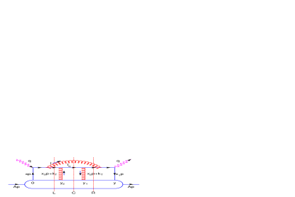
FIG. 1.: A typical diagram for quark-gluon re-scattering processes with three possible cuts, central(C), left(L) and right(R).

We will employ the generalized factorization of multiple scattering processes [14]. In this approximation, the double scattering contribution to radiative correction from processes like the one illustrated in Fig. 1 can be written in the following form,

$$\frac{dW_{\mu\nu}^{D}}{dz_{h}} = \sum_{q}\,\int_{z_{h}}^{1}\frac{dz}{z}D_{q\rightarrow h}(z_{h}/z)\int\frac{dy^{-}}{2\pi}\,dy_{1}^{-}dy_{2}^{-}\frac{1}{2}\,\langle A|\bar{\psi}_{q}(0)\,\gamma^{+}\,F_{\sigma}^{\ +}(y_{2}^{-})\,F^{+\sigma}(y_{1}^{-})\,\psi_{q}(y^{-})|A\rangle$$ (6)

$$\times \left(-\frac{1}{2}g^{\alpha\beta}\right)\left[\,\frac{1}{2}\,\frac{\partial^{2}}{\partial k_{T}^{\alpha}\partial k_{T}^{\beta}}\,\overline{H}^{D}_{\mu\nu}(y^{-},y_{1}^{-},y^{-}_{2},k_{T},p,q,z)\,\right]_{k_{T}=0}\,,$$ (7)

after collinear expansion of the hard partonic cross section with respect to the transverse momentum of the initial partons, where $\overline{H}^{D}_{\mu\nu}(y^{-},y_{1}^{-},y^{-}_{2},k_{T},p,q,z)$ is the Fourier transform of the partonic hard part $\widetilde{H}_{\mu\nu}(x,x_{1},x_{2},k_{T},p,q,z)$ in momentum space,

$$\overline{H}^{D}_{\mu\nu}(y^{-},y_{1}^{-},y^{-}_{2},k_{T},p,q,z) = \int dx\,\frac{dx_{1}}{2\pi}\,\frac{dx_{2}}{2\pi}\,e^{ix_{1}p^{+}y^{-}+ix_{2}p^{+}y_{1}^{-}+i(x-x_{1}-x_{2})p^{+}y_{2}^{-}}$$ (8)

$$\times\widetilde{H}^{D}_{\mu\nu}(x,x_{1},x_{2},k_{T},p,q,z)\ ,$$ (9)

and $k_{T}$ is the relative transverse momentum carried by the second parton in the double scattering. This is the leading term in the collinear expansion that contributes to the double scattering process. The first term in the collinear expansion gives the eikonal contribution to the leading-twist results, making the matrix element in the single scattering process gauge invariant, while the second (or linear) term vanishes for unpolarized initial and final states after integration over $k_{T}$.

The hard part of the partonic scattering for each diagram, $\widetilde{H}_{\mu\nu}(x,x_{1},x_{2},k_{T},p,q,z)$, always contains two $\delta$-functions from the on-shell conditions of the two cut-propagators. These $\delta$-functions, together with the contour integrations which contain different sets of poles in the un-cut propagators, will determine the values of the momentum fractions $x,x_{1},$ and $x_{2}$ [13]. The phase factors in $\overline{H}^{D}_{\mu\nu}(y^{-},y_{1}^{-},y^{-}_{2},k_{T},p,q,z)$ [Eq. (9)] can then be factored out, which will be combined with the partonic fields in Eq. (7) to form twist-four partonic matrix elements or two-parton correlations. The double scattering corrections in Eq. (7) can then be factorized into the product of fragmentation functions, twist-four partonic matrix elements and the partonic hard scattering cross section.

III Beyond Helicity Amplitude Approximation

To simplify the calculation of various cut-diagrams of double scattering and illustrate the underlying physical processes, helicity amplitude approximation was used in Ref. [13]. In this approximation, one neglects the transverse recoil induced by the scattering and consider only the part of the amplitudes in which quarks’ helicity is unchanged in the scattering. The final results will agree with the complete calculation in the limit of soft radiation.

Take photon bremsstrahlung for example. A complete calculation of photon radiation induced by a single scattering with transverse momentum transfer $k_{T}$ gives a spectra

$$\frac{dN}{d\ell_{T}^{2}dz}=\frac{\alpha}{2\pi}\left[\frac{\vec{\ell}_{T}}{\ell_{T}^{2}}-\frac{\vec{\ell}_{T}+(1-z)\vec{k}_{T}}{(\vec{\ell}_{T}+(1-z)\vec{k}_{T})^{2}}\right]^{2}\frac{1+z^{2}}{1-z}\;\;.$$ (10)

Here we denote the momentum of the photon (or gluon in QCD) to be $\ell$ which carries $1-z$ momentum fraction of the struck quark. Under helicity amplitude approximation, the splitting function will become $2/(1-z)$ and furthermore the term $(1-z)k_{T}$ in the final state radiation amplitude will be neglected. The interference between initial and final state radiation will effectively reduce the photon radiation spectrum to zero, apparently not a precise approximation. In QCD, the corresponding gluon radiation has similar amplitudes, except additional color matrices. Because the gluon exchange in the scattering transfers color, the emitted gluon in the initial and final state radiation can carry different colors. In this case, there is no complete destructive interference between initial and final state radiation as in QED. The helicity amplitude approximation is, therefore, a better approximation in QCD than in QED. However, it still neglects the corrections which contribute the most in photon radiation in QED. This finite correction is what we will study in this paper.

We first consider the contribution from Fig. 1 in detail and will list the results of other diagrams afterwards. Using the conventional Feynman rule, one can write down the hard partonic part of the central cut-diagram of Fig. 1 [13],

$$\overline{H}^{D}_{C\,\mu\nu}(y^{-},y_{1}^{-},y_{2}^{-},k_{T},p,q,z) = \int dx\frac{dx_{1}}{2\pi}\frac{dx_{2}}{2\pi}e^{ix_{1}p^{+}y^{-}+ix_{2}p^{+}y_{1}^{-}+i(x-x_{1}-x_{2})p^{+}y_{2}^{-}}\int\frac{d^{4}\ell}{(2\pi)^{4}}$$ (11)

$$\times \frac{1}{2}{\rm Tr}\left[p\cdot\gamma\gamma_{\mu}p^{\sigma}p^{\rho}\widehat{H}_{\sigma\rho}\gamma_{\nu}\right]2\pi\delta_{+}(\ell^{2})\,\delta(1-z-\frac{\ell^{-}}{q^{-}})\;.$$ (12)

$$\widehat{H}_{\sigma\rho} = \frac{C_{F}}{2N_{c}}g^{4}\frac{\gamma\cdot(q+x_{1}p)}{(q+x_{1}p)^{2}-i\epsilon}\,\gamma_{\alpha}\,\frac{\gamma\cdot(q+x_{1}p-\ell)}{(q+x_{1}p-\ell)^{2}-i\epsilon}\,\gamma_{\sigma}\gamma\cdot\ell_{q}\,\gamma_{\rho}$$ (13)

$$\times \varepsilon^{\alpha\beta}(\ell)\frac{\gamma\cdot(q+xp-\ell)}{(q+xp-\ell)^{2}+i\epsilon}\,\gamma_{\beta}\,\frac{\gamma\cdot(q+xp)}{(q+xp)^{2}+i\epsilon}\,\,2\pi\delta_{+}(\ell_{q}^{2})\,,$$ (14)

where $\varepsilon^{\alpha\beta}(\ell)$ is the polarization tensor of a gluon propagator in an axial gauge, $n\cdot A=0$ with $n=[1,0^{-},\vec{0}_{\perp}]$, and $\ell$, $\ell_{q}=q+(x_{1}+x_{2})p+k_{T}-\ell$ are the 4-momenta carried by the gluon and the final quark, respectively. $z=\ell_{q}^{-}/q^{-}$ is the fraction of longitudinal momentum (the large minus component) carried by the final quark.

To simplify the calculation, we also apply the collinear approximation to complete the trace of the product of $\gamma$-matrices,

$$p^{\sigma}\widehat{H}_{\sigma\rho}p^{\rho}\approx\gamma\cdot\ell_{q}\,\frac{1}{4\ell_{q}^{-}}{\rm Tr}\left[\gamma^{-}p^{\sigma}\widehat{H}_{\sigma\rho}p^{\rho}\right]\;.$$ (15)

After carrying out momentum integration in $x$, $x_{1}$, $x_{2}$ and $\ell^{\pm}$ with the help of contour integration and $\delta$-functions, the partonic hard part can be factorized into the production of $\gamma$-quark scattering matrix $H^{(0)}_{\mu\nu}(x,p,q)$ [Eq. (5)] and the quark-gluon rescattering part $\overline{H}^{D}$,

$$\overline{H}^{D}_{\mu\nu}(y^{-},y_{1}^{-},y_{2}^{-},k_{T},p,q,z)=\int dxH^{(0)}_{\mu\nu}(x,p,q)\ \overline{H}^{D}(y^{-},y_{1}^{-},y_{2}^{-},k_{T},x,p,q,z)\,.$$ (16)

Contributions from all the diagrams have this factorized from. Therefore, we will only list the rescattering part $\overline{H}^{D}$ for different diagrams in the following. For the central-cut diagram in Fig. 1 it reads [13],

$$\overline{H}^{D}_{C(Fig.\ref{fig1})}(y^{-},y_{1}^{-},y_{2}^{-},k_{T},x,p,q,z) = \int\frac{d\ell_{T}^{2}}{\ell_{T}^{2}}\,\frac{\alpha_{s}}{2\pi}\,C_{F}\frac{1+z^{2}}{1-z}$$ (17)

$$\times \frac{2\pi\alpha_{s}}{N_{c}}\overline{I}_{C(Fig.\ref{fig1})}(y^{-},y_{1}^{-},y_{2}^{-},\ell_{T},k_{T},x,p,q,z)\,,$$ (18)

$$\overline{I}_{C(Fig.\ref{fig1})}(y^{-},y_{1}^{-},y_{2}^{-},\ell_{T},k_{T},x,p,q,z) = e^{i(x+x_{L})p^{+}y^{-}+ix_{D}p^{+}(y_{1}^{-}-y_{2}^{-})}\theta(-y_{2}^{-})\theta(y^{-}-y_{1}^{-})$$ (19)

$$\times (1-e^{-ix_{L}p^{+}y_{2}^{-}})(1-e^{-ix_{L}p^{+}(y^{-}-y_{1}^{-})})\;.$$ (20)

Here, the fractional momentum is defined as

$$x_{L} = \frac{\ell_{T}^{2}}{2p^{+}q^{-}z(1-z)}\,\,,\,\,x_{D}=\frac{k_{T}^{2}-2\vec{k}_{T}\cdot\vec{\ell}_{T}}{2p^{+}q^{-}z}\,,$$ (21)

and $x=x_{B}=Q^{2}/2p^{+}q^{-}$ is the Bjorken variable.

The above contribution resembles the cross section of dipole scattering and contains essentially four terms. The first diagonal term corresponds to the so-called hard-soft process where the gluon radiation is induced by the hard scattering between the virtual photon and an initial quark with momentum fraction $x$. The quark is knocked off-shell by the virtual photon and becomes on-shell again after radiating a gluon. Afterwards the on-shell quark (or the radiated gluon) will have a secondary scattering with another soft gluon from the nucleus. The second diagonal term is due to the so-called double hard process where the quark is on-shell after the first hard scattering with the virtual photon. The gluon radiation is then induced by the scattering of the quark with another gluon that carries finite momentum fraction $x_{L}+x_{D}$. The other two off-diagonal terms are interferences between hard-soft and double hard processes. In the limit of collinear radiation ($x_{L}\rightarrow 0$) or when the formation time of the gluon radiation, $\tau_{f}\equiv 1/x_{L}p^{+}$, is much larger than the nuclear size, the two processes have destructive interference, leading to the LPM interference effect.

One can similarly obtain the rescattering part $\overline{H}^{D}$ of other central-cut diagrams (a-d) in Fig. 2:

$$\overline{H}^{D}_{C(a)}(y^{-},y_{1}^{-},y_{2}^{-},k_{T},x,p,q,z) = \int\frac{d\ell_{T}^{2}}{(\vec{\ell_{T}}-\vec{k_{T}})^{2}}\,\frac{\alpha_{s}}{2\pi}\,C_{A}\frac{1+z^{2}}{1-z}$$ (22)

$$\times \frac{2\pi\alpha_{s}}{N_{c}}\overline{I}_{C(a)}(y^{-},y_{1}^{-},y_{2}^{-},\ell_{T},k_{T},x,p,q,z)\,,$$ (23)

$$\overline{I}_{C(a)}(y^{-},y_{1}^{-},y_{2}^{-},\ell_{T},k_{T},x,p,q,z) = e^{i(x+x_{L})p^{+}y^{-}+ix_{D}p^{+}(y_{1}^{-}-y_{2}^{-})}\theta(-y_{2}^{-})\theta(y^{-}-y_{1}^{-})$$ (24)

$$\times [e^{ix_{D}p^{+}y_{2}^{-}/(1-z)}-e^{-ix_{L}p^{+}y_{2}^{-}}]$$ (25)

$$\times [e^{ix_{D}p^{+}(y^{-}-y_{1}^{-})/(1-z)}-e^{-ix_{L}p^{+}(y^{-}-y_{1}^{-})}]\,,$$ (26)

$$\overline{H}^{D}_{C(b)}(y^{-},y_{1}^{-},y_{2}^{-},k_{T},x,p,q,z) = \int\frac{d\ell_{T}^{2}}{(\vec{\ell_{T}}-(1-z)\vec{k_{T}})^{2}}\,\frac{\alpha_{s}}{2\pi}\,C_{F}\frac{1+z^{2}}{1-z}$$ (27)

$$\times \frac{2\pi\alpha_{s}}{N_{c}}\overline{I}_{C(b)}(y^{-},y_{1}^{-},y_{2}^{-},\ell_{T},k_{T},x,p,q,z)\,,$$ (28)

$$\overline{I}_{C(b)}(y^{-},y_{1}^{-},y_{2}^{-},\ell_{T},k_{T},x,p,q,z) = e^{i(x+x_{L})p^{+}y^{-}+ix_{D}p^{+}(y_{1}^{-}-y_{2}^{-})}\theta(-y_{2}^{-})\theta(y^{-}-y_{1}^{-})$$ (29)

$$\times e^{-ix_{L}p^{+}(y^{-}-y_{1}^{-})}e^{-ix_{L}p^{+}y_{2}^{-}}\,,$$ (30)

$$\overline{H}^{D}_{C(c)}(y^{-},y_{1}^{-},y_{2}^{-},k_{T},x,p,q,z) = \int d\ell_{T}^{2}\frac{(\vec{\ell_{T}}-\vec{k_{T}})\cdot(\vec{\ell_{T}}-(1-z)\vec{k_{T}})}{(\vec{\ell_{T}}-\vec{k_{T}})^{2}(\vec{\ell_{T}}-(1-z)\vec{k_{T}})^{2}}\,\frac{\alpha_{s}}{2\pi}\,\frac{C_{A}}{2}\frac{1+z^{2}}{1-z}$$ (31)

$$\times \frac{2\pi\alpha_{s}}{N_{c}}\overline{I}_{C(c)}(y^{-},y_{1}^{-},y_{2}^{-},\ell_{T},k_{T},x,p,q,z)\,,$$ (32)

$$\overline{I}_{C(c)}(y^{-},y_{1}^{-},y_{2}^{-},\ell_{T},k_{T},x,p,q,z) = e^{i(x+x_{L})p^{+}y^{-}+ix_{D}p^{+}(y_{1}^{-}-y_{2}^{-})}\,\theta(-y_{2}^{-})\theta(y^{-}-y_{1}^{-})$$ (33)

$$\times e^{-ix_{L}p^{+}y_{2}^{-}}$$ (34)

$$\times [e^{ix_{D}p^{+}(y^{-}-y_{1}^{-})/(1-z)}-e^{-ix_{L}p^{+}(y^{-}-y_{1}^{-})}]\,,$$ (35)

$$\overline{H}^{D}_{C(d)}(y^{-},y_{1}^{-},y_{2}^{-},k_{T},x,p,q,z) = \int d\ell_{T}^{2}\frac{(\vec{\ell_{T}}-\vec{k_{T}})\cdot(\vec{\ell_{T}}-(1-z)\vec{k_{T}})}{(\vec{\ell_{T}}-\vec{k_{T}})^{2}(\vec{\ell_{T}}-(1-z)\vec{k_{T}})^{2}}\,\frac{\alpha_{s}}{2\pi}\,\frac{C_{A}}{2}\frac{1+z^{2}}{1-z}$$ (36)

$$\times \frac{2\pi\alpha_{s}}{N_{c}}\overline{I}_{C(d)}(y^{-},y_{1}^{-},y_{2}^{-},\ell_{T},k_{T},x,p,q,z)\,,$$ (37)

$$\overline{I}_{C(d)}(y^{-},y_{1}^{-},y_{2}^{-},\ell_{T},k_{T},x,p,q,z) = e^{i(x+x_{L})p^{+}y^{-}+ix_{D}p^{+}(y_{1}^{-}-y_{2}^{-})}\,\theta(-y_{2}^{-})\theta(y^{-}-y_{1}^{-})$$ (38)

$$\times e^{-ix_{L}p^{+}(y^{-}-y_{1}^{-})}$$ (39)

$$\times [e^{ix_{D}p^{+}y_{2}^{-}/(1-z)}-e^{-ix_{L}p^{+}y_{2}^{-}}]\,.$$ (40)

To complete the calculation we also have to consider the asymmetrical-cut diagrams(left cut and right cut) that represent interferences between single and triple scatterings. They can be obtained with similar procedures. We list the rescattering part $\overline{H}^{D}$ of all those asymmetrical-cut diagrams in the Appendix.

To obtain the double scattering contribution to the semi-inclusive processes of hadron production in Eq. (7), one will then have to calculate the second derivatives of the rescattering part $\overline{H}^{D}$.

After a closer examination of these rescattering parts, one can find that all contributions from the asymmetrical-cut diagrams have the form as

$$\overline{H}^{D}_{asym}=\frac{\vec{\ell_{T}}\cdot(\vec{\ell_{T}}-f(z)\vec{k_{T}})}{\ell_{T}^{2}(\vec{\ell_{T}}-f(z)\vec{k_{T}})^{2}}e^{iXp^{+}Y^{-}},$$ (41)

where $f(z)=0,\,1,\,1-z,\,z$ is only a function of $z$, $X$ is the longitudinal momentum fraction and $Y^{-}$ the spatial coordinates. One can prove that the second derivative of the above expression vanishes at $k_{T}=0$,

$$\nabla^{2}_{k_{T}}\frac{\vec{\ell_{T}}\cdot(\vec{\ell_{T}}-f(z)\vec{k_{T}})}{\ell_{T}^{2}(\vec{\ell_{T}}-f(z)\vec{k_{T}})^{2}}=0\,.$$ (42)

Therefore, all contributions from the asymmetrical-cut(right-cut and left-cut) diagrams will vanish after we make the second partial derivative with respect to $k_{T}$ when we keep only the leading terms up to ${\cal O}(x_{B}/Q^{2}\ell_{T}^{2})$,

$$\nabla^{2}_{k_{T}}\overline{H}^{D}_{asym}|_{k_{T}=0} = 0+{\cal O}(x_{B}/Q^{2}\ell_{T}^{2}).$$ (43)

In the same way we find that some of the central-cut diagrams will not contribute to the final results, either. In fact, after making the second partial derivative with respect to $k_{T}$ only four central-cut diagrams shown in Fig. 2 will contribute to the final result.

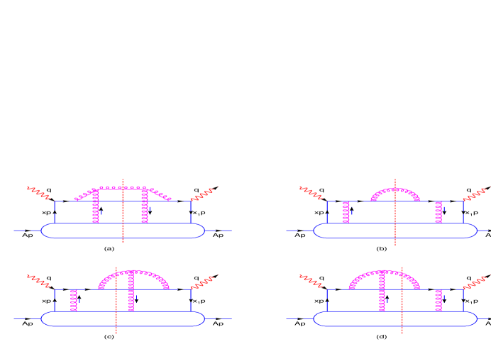
FIG. 2.: Four central-cut Diagrams that contribute to the final results.

Including only those contributions that does not vanish after second derivative with respect to $k_{T}$, we have

$$\nabla^{2}_{k_{T}}\overline{H}^{D}|_{k_{T}=0} = \int d\ell_{T}^{2}\frac{\alpha_{s}}{2\pi}\frac{1+z^{2}}{1-z}e^{i(x+x_{L})p^{+}y^{-}}\frac{2\pi\alpha_{s}}{N_{c}}\theta(-y_{2}^{-})\theta(y^{-}-y_{1}^{-})$$ (44)

$$\times \left[\frac{4C_{A}}{\ell_{T}^{4}}(1-e^{-ix_{L}p^{+}y_{2}^{-}})(1-e^{-ix_{L}p^{+}(y^{-}-y_{1}^{-})})\right.$$ (45)

$$+ \frac{4C_{F}(1-z)^{2}}{\ell_{T}^{4}}e^{-ix_{L}p^{+}(y^{-}-y_{1}^{-})}e^{-ix_{L}p^{+}y_{2}^{-}}$$ (46)

$$+ \frac{2C_{A}(1-z)}{\ell_{T}^{4}}e^{-ix_{L}p^{+}y_{2}^{-}}(1-e^{-ix_{L}p^{+}(y^{-}-y_{1}^{-})})$$ (47)

$$+ \left.\frac{2C_{A}(1-z)}{\ell_{T}^{4}}e^{-ix_{L}p^{+}(y^{-}-y_{1}^{-})}(1-e^{-ix_{L}p^{+}y_{2}^{-}})+{\cal O}(x_{B}/Q^{2}\ell_{T}^{2})\right]\,$$ (48)

The first term at the right-hand side in Eq. (48) comes from the contribution of $\overline{H}^{D}_{C(a)}$ which is the main contribution in the previous calculation [13] with helicity amplitude approximation. It contains hard-soft, double hard processes and their interferences. The other three terms come from diagram (b),(c),(d) of Fig. 2 respectively. They constitute corrections to the first term in powers of $1-z$. The second term that are proportional to $(1-z)^{2}$ is from the final state radiation from the quark in the double hard process in Fig. 2-(b). This term is the only contribution to the finite photon spectra in the corresponding QED bremsstrahlung. The third and fourth terms are the results of the interference of the final state radiation from the quark and other radiation processes (initial state radiation and radiation from the gluon line). They contain both double hard processes and interferences between hard-soft and double hard processes in Fig. 2-(c) and (d). In the limit of soft gluon radiation, $(1-z)\rightarrow 0$, these three terms can be neglected and we recover the result in the helicity amplitude approximation [13].

IV Modified Fragmentation Function and Parton Energy Loss

Substituting Eq. (48) into Eq. (16), Eq. (7) and adding the gluon fragmentation processes, we have the semi-inclusive tensor from double quark-gluon scattering including the contribution beyond the helicity amplitude approximation,

$$\frac{W_{\mu\nu}^{D,q}}{dz_{h}} = \sum_{q}\,\int dxH^{(0)}_{\mu\nu}(xp,q)\int_{z_{h}}^{1}\frac{dz}{z}D_{q\rightarrow h}(z_{h}/z)\frac{\alpha_{s}}{2\pi}C_{A}\frac{1+z^{2}}{1-z}$$ (49)

$$\times \int\frac{d\ell_{T}^{2}}{\ell_{T}^{4}}\frac{2\pi\alpha_{s}}{N_{c}}\left[T^{A}_{qg}(x,x_{L})+(1-z)T^{A(1)}_{qg}(x,x_{L})+\frac{C_{F}}{C_{A}}(1-z)^{2}T^{A(2)}_{qg}(x,x_{L})\right]$$ (50)

$$+ (g-{\rm fragmentation})+({\rm virtual\,\,corrections})\,,$$ (51)

where

$$T^{A}_{qg}(x,x_{L}) = \int\frac{dy^{-}}{2\pi}\,dy_{1}^{-}dy_{2}^{-}(1-e^{-ix_{L}p^{+}y_{2}^{-}})(1-e^{-ix_{L}p^{+}(y^{-}-y_{1}^{-})})e^{i(x+x_{L})p^{+}y^{-}}$$ (53)

$$\frac{1}{2}\langle A|\bar{\psi}_{q}(0)\,\gamma^{+}\,F_{\sigma}^{\ +}(y_{2}^{-})\,F^{+\sigma}(y_{1}^{-})\,\psi_{q}(y^{-})|A\rangle\theta(-y_{2}^{-})\theta(y^{-}-y_{1}^{-})\;\;,$$

$$T^{A(1)}_{qg}(x,x_{L}) = \int\frac{dy^{-}}{2\pi}\,dy_{1}^{-}dy_{2}^{-}\left[e^{-ix_{L}p^{+}(y^{-}-y^{-}_{1})}+e^{-ix_{L}p^{+}y^{-}_{2}}-2e^{-ix_{L}p^{+}(y^{-}-y^{-}_{1}+y_{2}^{-})}\right]$$ (55)

$$e^{i(x+x_{L})p^{+}y^{-}}\frac{1}{4}\langle A|\bar{\psi}_{q}(0)\,\gamma^{+}\,F_{\sigma}^{\ +}(y_{2}^{-})\,F^{+\sigma}(y_{1}^{-})\,\psi_{q}(y^{-})|A\rangle\theta(-y_{2}^{-})\theta(y^{-}-y_{1}^{-})\;\;,$$

$$T^{A(2)}_{qg}(x,x_{L}) = \int\frac{dy^{-}}{2\pi}\,dy_{1}^{-}dy_{2}^{-}e^{ixp^{+}y^{-}+ix_{L}p^{+}(y^{-}_{1}-y^{-}_{2})}$$ (57)

$$\frac{1}{2}\langle A|\bar{\psi}_{q}(0)\,\gamma^{+}\,F_{\sigma}^{\ +}(y_{2}^{-})\,F^{+\sigma}(y_{1}^{-})\,\psi_{q}(y^{-})|A\rangle\theta(-y_{2}^{-})\theta(y^{-}-y_{1}^{-})$$

are twist-four parton matrix elements of the nucleus. Apparently these parton matrix elements are not independent of each other. $T^{A}_{qg}(x,x_{L})$ has the complete four terms of soft-hard, double hard processes and their interferences. Therefore it contains essentially four independent parton matrix elements. $T^{A(1)}_{qg}(x,x_{L})$ and $T^{A(2)}_{gq}(x,x_{L})$ are the results of the corrections beyond helicity amplitude approximation. But these two matrix elements are already contained in $T^{A}_{qg}(x,x_{L})$.

During the collinear expansion, we have kept $\ell_{T}$ finite and took the limit $k_{T}\rightarrow 0$. As a consequence, the gluon field in one of the twist-four parton matrix elements in Eqs. (53)-(57) carries zero momentum in the soft-hard process. However, the gluon distribution $xf_{g}(x)$ at $x=0$ is not defined in QCD. As argued in Ref. [13], this is due to the omission of higher order terms in the collinear expansion. As a remedy to the problem, a subset of the higher-twist terms in the collinear expansion can be resummed to restore the phase factors such as $\exp(ix_{T}p^{+}y^{-})$, where $x_{T}\equiv\langle k_{T}^{2}\rangle/2p^{+}q^{-}z$ is related to the intrinsic transverse momentum of the initial partons. As a result, soft gluon fields in the parton matrix elements will carry a fractional momentum $x_{T}$.

Using the factorization approximation [13, 14, 17] we can relate the twist-four parton matrix elements of the nucleus to the twist-two parton distributions of nucleons and the nucleus,

$$T^{A}_{qg}(x,x_{L})=\frac{C}{x_{A}}(1-e^{-x_{L}^{2}/x_{A}^{2}})[f_{q}^{A}(x+x_{L})\,x_{T}f_{g}^{N}(x_{T})+f_{q}^{A}(x)(x_{L}+x_{T})f_{g}^{N}(x_{L}+x_{T})]\,$$ (58)

where C is a constant, $x_{A}=1/MR_{A}$, $f_{q}^{A}(x)$ is the quark distribution inside a nucleus, and $f_{g}^{N}(x)$ is the gluon distribution inside a nucleon. A Gaussian distribution in the light-cone coordinates was assumed for the nuclear distribution, $\rho(y^{-})=\rho_{0}\exp({y^{-}}^{2}/2{R^{-}_{A}}^{2})$, where $R^{-}_{A}=\sqrt{2}R_{A}M/p^{+}$ and $M$ is the nucleon mass. We should emphasize that the twist-four matrix elements is proportional to $1/x_{A}=R_{A}M$, or the nuclear size [17].

Notice that the off-diagonal matrix elements that correspond to the interferences between hard-soft and double hard processes is suppressed by a factor of $\exp(-x_{L}^{2}/x_{A}^{2})$. This is because in the interferences between double-hard and hard-soft processes, there is actually momentum flow of $x_{L}p^{+}$ between the two nucleons where the initial quark and gluon come from. Without strong long range two-nucleon correlation inside a nucleus, the amount of momentum flow $x_{L}p^{+}$ should then be restricted to the amount allowed by the uncertainty principle, $1/R^{-}_{A}\sim p^{+}/R_{A}M$. Similarly, the other two parton matrix elements in Eqs. (55) and (57) can be approximated as

$$T^{A(1)}_{qg}(x,x_{L}) = \frac{C}{2x_{A}}\left\{\left[f_{q}^{A}(x+x_{L})\,x_{T}f_{g}^{N}(x_{T})+f_{q}^{A}(x)(x_{L}+x_{T})f_{g}^{N}(x_{L}+x_{T})\right]e^{-x_{L}^{2}/x_{A}^{2}}\right.$$ (59)

$$- \left.2f_{q}^{A}(x)(x_{L}+x_{T})f_{g}^{N}(x_{L}+x_{T})\right\}\,,$$ (60)

$$T^{A(2)}_{qg}(x,x_{L}) = \frac{C}{x_{A}}f_{q}^{A}(x)(x_{L}+x_{T})f_{g}^{N}(x_{L}+x_{T})\,.$$ (61)

From the above estimate of the matrix elements, both $T^{A}_{qg}(x,x_{L})$ and $T^{A(1)}_{qg}(x,x_{L})$ contain a factor $1-e^{-x_{L}^{2}/x_{A}^{2}}$ because of the LPM interference effect. Such an interference factor will effectively cut off the integration over the transverse momentum at $x_{L}\sim x_{A}$ in Eq. (51). As we will show later in the calculation of the effective energy loss, the integration with such a restriction in the transverse momentum due to LPM interference effect will give rise to a factor $1/x_{A}$ in addition to the coefficient $f^{A}_{q}(x)/x_{A}$. Consequently, contributions from double scattering in Eq. (51) that are associated with $T^{A}_{qg}(x,x_{L})$ and $T^{A(1)}_{qg}(x,x_{L})$ will be proportional to $R_{A}^{2}f^{A}_{q}(x)$. These are the leading double scattering contributions in the limit of large nuclear size. On the other hand, the third term $T^{A(2)}_{qg}(x,x_{L})$ in Eq. (51), which does not contain any interference effect, will only contribute to a correction that is proportional to $R_{A}f^{A}_{q}(x)$. In the limit of a large nucleus, $A^{1/3}\gg 1$, we will neglect this term in the double scattering processes. It is interesting to point out, however, that the physical process associated with this term is totally responsible for the non-vanishing photon spectra in QED bremsstrahlung which otherwise vanishes in the helicity amplitude approximation. As we can see, the leading correction beyond helicity amplitude approximation comes from the interference between this process and other radiation processes that contribute to the leading result in the first term.

The virtual correction in Eq. (51) can be obtained via unitarity requirement similarly as in Ref. [13]. Including these virtual corrections and the single scattering contribution, we can rewrite the semi-inclusive tensor in terms of a modified fragmentation function $\widetilde{D}_{q\rightarrow h}(z_{h},\mu^{2})$,

$$\frac{dW_{\mu\nu}}{dz_{h}}=\sum_{q}\int dx\widetilde{f}_{q}^{A}(x,\mu_{I}^{2})H^{(0)}_{\mu\nu}(x,p,q)\widetilde{D}_{q\rightarrow h}(z_{h},\mu^{2})$$ (62)

where $\widetilde{f}_{q}^{A}(x,\mu_{I}^{2})$ is the quark distribution functions which in principle should also include the higher-twist contribution [18] of the initial state scattering. The modified effective quark fragmentation function is defined as

$$\widetilde{D}_{q\rightarrow h}(z_{h},\mu^{2}) \equiv D_{q\rightarrow h}(z_{h},\mu^{2})+\int_{0}^{\mu^{2}}\frac{d\ell_{T}^{2}}{\ell_{T}^{2}}\frac{\alpha_{s}}{2\pi}\int_{z_{h}}^{1}\frac{dz}{z}\left[\Delta\gamma_{q\rightarrow qg}(z,x,x_{L},\ell_{T}^{2})D_{q\rightarrow h}(z_{h}/z)\right.$$ (63)

$$+ \left.\Delta\gamma_{q\rightarrow gq}(z,x,x_{L},\ell_{T}^{2})D_{g\rightarrow h}(z_{h}/z)\right]\,,$$ (64)

where $D_{q\rightarrow h}(z_{h},\mu^{2})$ and $D_{g\rightarrow h}(z_{h},\mu^{2})$ are the leading-twist fragmentation functions. The modified splitting functions are given as

$$\Delta\gamma_{q\rightarrow qg}(z,x,x_{L},\ell_{T}^{2}) = \left[\frac{1+z^{2}}{(1-z)_{+}}T^{A(m)}_{qg}(x,x_{L})+\delta(1-z)\Delta T^{A(m)}_{qg}(x,\ell_{T}^{2})\right]\frac{2\pi\alpha_{s}C_{A}}{\ell_{T}^{2}N_{c}\widetilde{f}_{q}^{A}(x,\mu_{I}^{2})}\,,$$ (65)

$$\Delta\gamma_{q\rightarrow gq}(z,x,x_{L},\ell_{T}^{2}) = \Delta\gamma_{q\rightarrow qg}(1-z,x,x_{L},\ell_{T}^{2}),$$ (66)

$$\Delta T^{A(m)}_{qg}(x,\ell_{T}^{2}) \equiv \int_{0}^{1}dz\frac{1}{1-z}\left[2T^{A(m)}_{qg}(x,x_{L})|_{z=1}-(1+z^{2})T^{A(m)}_{qg}(x,x_{L})\right]\,,$$ (67)

$$T^{A(m)}_{qg}(x,x_{L}) \equiv T^{A}_{qg}(x,x_{L})+(1-z)T^{A(1)}_{qg}(x,x_{L})\,.$$ (68)

The above modified fragmentation function is almost the same as in the previous calculation with helicity amplitude approximation, except that the twist-four parton matrix element $T^{A}_{qg}(x,x_{L})$ is replaced by a modified one $T^{A(m)}_{qg}(x,x_{L})$ in Eq. (68). One can then calculate numerically the modified fragmentation function as in Refs. [12, 13]. To further simplify the calculation, we assume $x_{T}\ll x_{L}\ll x$. The modified parton matrix elements can be approximated by

$$T^{A(m)}_{qg}(x,x_{L})\approx\frac{\widetilde{C}}{x_{A}}(1-e^{-x_{L}^{2}/x_{A}^{2}})f_{q}^{A}(x)\left[1-\frac{1-z}{2}\right],$$ (69)

where $\widetilde{C}\equiv 2Cx_{T}f^{N}_{g}(x_{T})$ is a coefficient which should in principle depends on $Q^{2}$ and $x_{T}$. Here we will simply take it as a constant. The new correction term in this calculation is thus negative in the modified splitting function. This will reduce the nuclear suppression of hadron spectra at large values of $z$ and thus reduce the effective quark energy loss.

Because of momentum conservation, the fractional momentum in a nucleon is limited to $x_{L}<1$. Though the Fermi motion effect in a nucleus can allow $x_{L}>1$, the parton distribution in this region is still significant suppressed. It therefore provides a natural cut-off for $x_{L}$ in the integration over $z$ and $\ell_{T}$ in Eq. (64). Shown in Fig. 3 are the calculated nuclear modification factor for the quark fragmentation function $D_{A}(z,Q^{2})/D_{N}(z,Q^{2})$ inside a nucleus with $A=100$. In this numerical evaluation, we have taken $\widetilde{C}=0.006$ GeV² which was fitted to the HERMES experimental data [12]. The dashed curve is for the modified fragmentation function in the helicity amplitude approximation and the solid curve is obtained with the new correction term. Apparently, the new correction term reduces the nuclear modification, though the reduction is not very significant.

FIG. 3.: Calculated nuclear modification factor for the quark fragmentation in a nucleus (A=100). The solid line is the current calculation with the new correction term. The dashed line is the previous result with helicity amplitude approximation.

Similarly, we can also calculate the effective quark energy loss, which is defined as the energy carried away by the radiated gluon,

$$\langle\Delta z_{g}\rangle(x_{B},\mu^{2}) = \int_{0}^{\mu^{2}}\frac{d\ell_{T}^{2}}{\ell_{T}^{2}}\int_{0}^{1}dz\frac{\alpha_{s}}{2\pi}z\,\Delta\gamma_{q\rightarrow gq}(z,x_{B},x_{L},\ell_{T}^{2})$$ (70)

$$= \frac{C_{A}\alpha_{s}^{2}}{N_{c}}\int_{0}^{\mu^{2}}\frac{d\ell_{T}^{2}}{\ell_{T}^{4}}\int_{0}^{1}dz[1+(1-z)^{2}]\frac{T^{A(m)}_{qg}(x_{B},x_{L})}{\widetilde{f}_{q}^{A}(x_{B},\mu_{I}^{2})}\,.$$ (71)

We separate the parton energy loss as two parts

$$\langle\Delta z_{g}\rangle(x_{B},\mu^{2})=\langle\Delta z_{g}\rangle_{heli}(x_{B},\mu^{2})+\langle\Delta z_{g}\rangle_{corr}(x_{B},\mu^{2}),$$ (72)

where $\langle\Delta z_{g}\rangle_{heli}(x_{B},\mu^{2})$ is the leading quark energy loss with helicity amplitude approximation [13], and $\langle\Delta z_{g}\rangle_{corr}(x_{B},\mu^{2})$ is the new correction to the quark energy loss in this calculation. Using the approximation for the modified twist-four parton matrix elements in Eq. (69), we have

$$\langle\Delta z_{g}\rangle_{heli}(x_{B},\mu^{2}) = \widetilde{C}\frac{C_{A}\alpha_{s}^{2}}{N_{c}}\frac{x_{B}}{x_{A}Q^{2}}\int_{0}^{1}dz\frac{1+(1-z)^{2}}{z(1-z)}\int_{0}^{x_{\mu}}\frac{dx_{L}}{x_{L}^{2}}(1-e^{-x_{L}^{2}/x_{A}^{2}});$$ (73)

$$\langle\Delta z_{g}\rangle_{corr}(x_{B},\mu^{2}) = \widetilde{C}\frac{C_{A}\alpha_{s}^{2}}{N_{c}}\frac{x_{B}}{x_{A}Q^{2}}\int_{0}^{1}dz\frac{1+(1-z)^{2}}{z(1-z)}\int_{0}^{x_{\mu}}\frac{dx_{L}}{x_{L}^{2}}(-\frac{z}{2})(1-e^{-x_{L}^{2}/x_{A}^{2}})\,,$$ (74)

where $x_{\mu}=\mu^{2}/2p^{+}q^{-}z(1-z)=x_{B}/z(1-z)$ if we choose the factorization scale as $\mu^{2}=Q^{2}$. When $x_{A}\ll x_{B}\ll 1$ we can estimate the leading quark energy loss roughly as

$$\langle\Delta z_{g}\rangle_{heli}(x_{B},\mu^{2}) \approx \widetilde{C}\frac{C_{A}\alpha_{s}^{2}}{N_{c}}\frac{x_{B}}{Q^{2}x_{A}^{2}}2\sqrt{\pi}[3\ln\frac{1-2x_{B}}{x_{B}}-1]\,,$$ (76)

$$\langle\Delta z_{g}\rangle_{corr}(x_{B},\mu^{2}) \approx -\widetilde{C}\frac{C_{A}\alpha_{s}^{2}}{N_{c}}\frac{x_{B}}{Q^{2}x_{A}^{2}}\sqrt{\pi}[\ln\frac{1-2x_{B}}{x_{B}}+\frac{1}{2}]\,.$$ (77)

Since $x_{A}=1/MR_{A}$, both of the energy loss $\langle\Delta z_{g}\rangle_{heli}$ and $\langle\Delta z_{g}\rangle_{corr}$ depend quadratically on the nuclear size. Adding them together, we have

$$\langle\Delta z_{g}\rangle(x_{B},\mu^{2}) \approx \frac{\tilde{C}\alpha_{s}^{2}}{N_{c}}\frac{x_{B}}{Q^{2}x_{A}^{2}}\sqrt{\pi}[5\ln\frac{1-2x_{B}}{x_{B}}-\frac{5}{2}]$$ (78)

$$\approx \frac{5}{6}\langle\Delta z_{g}\rangle_{heli}(x_{B},\mu^{2}),\ \ \ (x_{A}\ll x_{B}\ll 1)\,.$$ (79)

The new correction thus reduces the effective quark energy loss by approximately a factor of $5/6$ from the result with helicity amplitude approximation.

V Summary

We have extended an earlier study [13] on gluon radiation induced by multiple parton scattering in DIS off a nuclear target with a complete calculation beyond the helicity amplitude (or soft radiation) approximation. Working within the framework of the generalized factorization of twist-four processes, we obtained a new correction to the modified parton fragmentation functions. Such a new correction essentially results in a new term in the modified splitting function which is proportional to $(1-z)$. In the limit of helicity amplitude approximation $(1-z)\rightarrow 0$, this term vanishes and we recover the early results [13].

The new correction we obtained in this paper comes from the gluon radiation process (residual final state radiation from a quark after incomplete cancellation by the initial state radiation) that is actually responsible for the photon radiation in QED. However, the leading correction beyond the helicity amplitude approximation does not come from this process itself. Rather, it comes from the interference between this process and the other gluon radiation processes that are responsible for the result in the helicity amplitude approximation. Though it is not dominant for induced gluon radiation in QCD, it still make a finite contribution to the modified fragmentation function for a quark propagating inside a nuclear medium and to the effective quark energy loss. We found that it reduces the effective quark energy loss by a factor of $5/6$.

Appendix

In this Appendix we will list our complete calculation of quark-gluon double scattering in detail. There are total 23 cut diagrams which are illustrated in Figs. 4-14.

FIG. 4.:

In Fig. 4 there are three possible cuts(central cut, left cut and right cut). We get

$$\overline{H}^{D}_{Ap-1}(y^{-},y_{1}^{-},y_{2}^{-},k_{T},x,p,q,z) = \int\frac{d\ell_{T}^{2}}{\ell_{T}^{2}}\,\frac{\alpha_{s}}{2\pi}C_{F}\,\frac{1+z^{2}}{1-z}$$ (80)

$$\times \frac{2\pi\alpha_{s}}{N_{c}}\overline{I}_{Ap-1}(y^{-},y_{1}^{-},y_{2}^{-},\ell_{T},k_{T},x,p,q,z)\,,$$ (81)

where

$$\overline{I}_{Ap-1,C}(y^{-},y_{1}^{-},y_{2}^{-},\ell_{T},k_{T},x,p,q,z) = e^{i(x+x_{L})p^{+}y^{-}+ix_{D}p^{+}(y_{1}^{-}-y_{2}^{-})}\theta(-y_{2}^{-})\theta(y^{-}-y_{1}^{-})$$ (82)

$$\times (1-e^{-ix_{L}p^{+}y_{2}^{-}})(1-e^{-ix_{L}p^{+}(y^{-}-y_{1}^{-})})\;.$$ (83)

$$\overline{I}_{Ap-1,L}(y^{-},y_{1}^{-},y_{2}^{-},\ell_{T},k_{T},x,p,q,z)\, = -e^{i(x+x_{L})p^{+}y^{-}+ix_{D}p^{+}(y_{1}^{-}-y_{2}^{-})}\theta(y_{1}^{-}-y_{2}^{-})\theta(y^{-}-y_{1}^{-})$$ (84)

$$\times (1-e^{-ix_{L}p^{+}(y^{-}-y_{1}^{-})})\,,$$ (85)

$$\overline{I}_{Ap-1,R}(y^{-},y_{1}^{-},y_{2}^{-},\ell_{T},k_{T},x,p,q,z) = -e^{i(x+x_{L})p^{+}y^{-}+ix_{D}p^{+}(y_{1}^{-}-y_{2}^{-})}\theta(-y_{2}^{-})\theta(y_{2}^{-}-y_{1}^{-})$$ (86)

$$\times (1-e^{-ix_{L}p^{+}y_{2}^{-}})\,.$$ (87)

FIG. 5.:

In Fig. 5, there are two different cuts, central or left. So we obtain,

$$\overline{H}^{D}_{Ap-2}(y^{-},y_{1}^{-},y_{2}^{-},k_{T},x,p,q,z) = \int d\ell_{T}^{2}\frac{\vec{\ell_{T}}\cdot(\vec{\ell_{T}}-(1-z)\vec{k_{T}})}{\ell_{T}^{2}(\vec{\ell_{T}}-(1-z)\vec{k_{T}})^{2}}\,\frac{\alpha_{s}}{2\pi}\,(C_{F}-\frac{C_{A}}{2})\frac{1+z^{2}}{1-z}$$ (88)

$$\times \frac{2\pi\alpha_{s}}{N_{c}}\overline{I}_{Ap-2}(y^{-},y_{1}^{-},y_{2}^{-},\ell_{T},k_{T},x,p,q,z)\,,$$ (89)

$$\overline{I}_{Ap-2,C}(y^{-},y_{1}^{-},y_{2}^{-},\ell_{T},k_{T},x,p,q,z) = e^{i(x+x_{L})p^{+}y^{-}+ix_{D}p^{+}(y_{1}^{-}-y_{2}^{-})}\theta(-y_{2}^{-})\theta(y^{-}-y_{1}^{-})$$ (90)

$$\times [e^{-ix_{L}p^{+}(y^{-}-y_{1}^{-})}-e^{-ix_{L}p^{+}(y^{-}-y_{1}^{-}+y_{2}^{-})}]\,,$$ (91)

$$\overline{I}_{Ap-2,L}(y^{-},y_{1}^{-},y_{2}^{-},\ell_{T},k_{T},x,p,q,z) = e^{i(x+x_{L})p^{+}y^{-}+ix_{D}p^{+}(y_{1}^{-}-y_{2}^{-})}\theta(y^{-}-y_{1}^{-})\theta(y_{1}^{-}-y_{2}^{-})$$ (92)

$$\times [e^{-ix_{L}p^{+}(y^{-}-y_{2}^{-})+i(x_{D}^{0}-x_{D})p^{+}(y_{1}^{-}-y_{2}^{-})}-e^{-ix_{L}p^{+}(y^{-}-y_{1}^{-})}]\,,$$ (93)

where $x_{D}^{0}=k_{T}/2p^{+}q^{-}$.

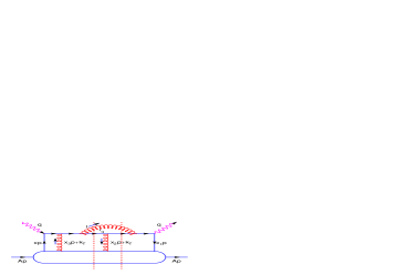
FIG. 6.:

As for the central cut and right cut of Fig. 6, we obtain

$$\overline{H}^{D}_{Ap-3}(y^{-},y_{1}^{-},y_{2}^{-},k_{T},x,p,q,z) = \int d\ell_{T}^{2}\frac{\vec{\ell_{T}}\cdot(\vec{\ell_{T}}-(1-z)\vec{k_{T}})}{\ell_{T}^{2}(\vec{\ell_{T}}-(1-z)\vec{k_{T}})^{2}}\,\frac{\alpha_{s}}{2\pi}\,(C_{F}-\frac{C_{A}}{2})\frac{1+z^{2}}{1-z}$$ (94)

$$\times \frac{2\pi\alpha_{s}}{N_{c}}\overline{I}_{Ap-3}(y^{-},y_{1}^{-},y_{2}^{-},\ell_{T},k_{T},x,p,q,z)\,,$$ (95)

$$\overline{I}_{Ap-3,C}(y^{-},y_{1}^{-},y_{2}^{-},\ell_{T},k_{T},x,p,q,z) = e^{i(x+x_{L})p^{+}y^{-}+ix_{D}p^{+}(y_{1}^{-}-y_{2}^{-})}\theta(-y_{2}^{-})\theta(y^{-}-y_{1}^{-})$$ (96)

$$\times [e^{-ix_{L}p^{+}y_{2}^{-}}-e^{-ix_{L}p^{+}(y^{-}-y_{1}^{-}+y_{2}^{-})}]\,,$$ (97)

$$\overline{I}_{Ap-3,R}(y^{-},y_{1}^{-},y_{2}^{-},\ell_{T},k_{T},x,p,q,z) = e^{i(x+x_{L})p^{+}y^{-}+ix_{D}p^{+}(y_{1}^{-}-y_{2}^{-})}\theta(-y_{2}^{-})\theta(y_{2}^{-}-y_{1}^{-})$$ (98)

$$\times [e^{-i(x_{D}^{0}-x_{D})p^{+}(y_{1}^{-}-y_{2}^{-})-ix_{L}p^{+}y_{1}^{-}}-e^{-ix_{L}p^{+}y_{2}^{-}}]\,.$$ (99)

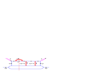
FIG. 7.:

There is only one cut (left cut) in Fig. 7 with the contribution,

$$\overline{H}^{D}_{Ap-4}(y^{-},y_{1}^{-},y_{2}^{-},k_{T},x,p,q,z) = \int\frac{d\ell_{T}^{2}}{\ell_{T}^{2}}\,\frac{\alpha_{s}}{2\pi}\,C_{F}\frac{1+z^{2}}{1-z}$$ (100)

$$\times \frac{2\pi\alpha_{s}}{N_{c}}\overline{I}_{Ap-4}(y^{-},y_{1}^{-},y_{2}^{-},\ell_{T},k_{T},x,p,q,z)\,,$$ (101)

$$\overline{I}_{Ap-4,L}(y^{-},y_{1}^{-},y_{2}^{-},\ell_{T},k_{T},x,p,q,z) = -e^{i(x+x_{L})p^{+}y^{-}+ix_{D}p^{+}(y_{1}^{-}-y_{2}^{-})}\theta(y^{-}-y_{1}^{-})\theta(y_{1}^{-}-y_{2}^{-})$$ (102)

$$\times e^{i(x_{D}^{0}-x_{D})p^{+}(y_{1}^{-}-y_{2}^{-})}e^{-ix_{L}p^{+}(y^{-}-y_{2}^{-})}\,.$$ (103)

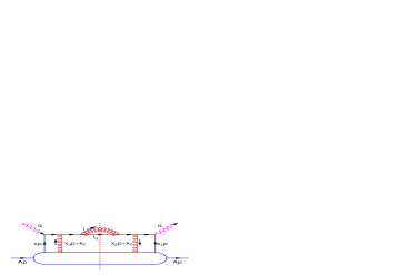
FIG. 8.:

As for Fig. 8, we get

$$\overline{H}^{D}_{Ap-5}(y^{-},y_{1}^{-},y_{2}^{-},k_{T},x,p,q,z) = \int\frac{d\ell_{T}^{2}}{(\vec{\ell_{T}}-(1-z)\vec{k_{T}})^{2}}\,\frac{\alpha_{s}}{2\pi}\,C_{F}\frac{1+z^{2}}{1-z}$$ (104)

$$\times \frac{2\pi\alpha_{s}}{N_{c}}\overline{I}_{Ap-5}(y^{-},y_{1}^{-},y_{2}^{-},\ell_{T},k_{T},x,p,q,z)\,,$$ (105)

$$\overline{I}_{Ap-5,C}(y^{-},y_{1}^{-},y_{2}^{-},\ell_{T},k_{T},x,p,q,z) = e^{i(x+x_{L})p^{+}y^{-}+ix_{D}p^{+}(y_{1}^{-}-y_{2}^{-})}\theta(-y_{2}^{-})\theta(y^{-}-y_{1}^{-})$$ (106)

$$\times e^{-ix_{L}p^{+}(y^{-}-y_{1}^{-})}e^{-ix_{L}p^{+}y_{2}^{-}}\,.$$ (107)

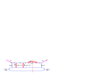
FIG. 9.:

The contribution from Fig. 9 is

$$\overline{H}^{D}_{Ap-6}(y^{-},y_{1}^{-},y_{2}^{-},k_{T},x,p,q,z) = \int\frac{d\ell_{T}^{2}}{\ell_{T}^{2}}\,\frac{\alpha_{s}}{2\pi}\,C_{F}\frac{1+z^{2}}{1-z}$$ (108)

$$\times \frac{2\pi\alpha_{s}}{N_{c}}\overline{I}_{Ap-6}(y^{-},y_{1}^{-},y_{2}^{-},\ell_{T},k_{T},x,p,q,z)\,,$$ (109)

$$\overline{I}_{Ap-6,R}(y^{-},y_{1}^{-},y_{2}^{-},\ell_{T},k_{T},x,p,q,z) = -e^{i(x+x_{L})p^{+}y^{-}+ix_{D}p^{+}(y_{1}^{-}-y_{2}^{-})}\theta(-y_{2}^{-})\theta(y_{2}^{-}-y_{1}^{-})$$ (110)

$$\times e^{i(x_{D}^{0}-x_{D})p^{+}(y_{1}^{-}-y_{2}^{-})}e^{-ix_{L}p^{+}y_{1}^{-}}\,.$$ (111)

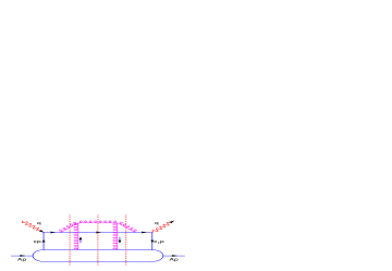
FIG. 10.:

As for the processes in Fig. 10 we have three possible cuts. Thus the contributions can be written as

$$\overline{H}^{D}_{Ap-7,C}(y^{-},y_{1}^{-},y_{2}^{-},k_{T},x,p,q,z) = \int\frac{d\ell_{T}^{2}}{(\vec{\ell_{T}}-\vec{k_{T}})^{2}}\,\frac{\alpha_{s}}{2\pi}\,C_{A}\frac{1+z^{2}}{1-z}$$ (112)

$$\times \frac{2\pi\alpha_{s}}{N_{c}}\overline{I}_{Ap-7,C}(y^{-},y_{1}^{-},y_{2}^{-},\ell_{T},k_{T},x,p,q,z)\,,$$ (113)

$$\overline{I}_{Ap-7,C}(y^{-},y_{1}^{-},y_{2}^{-},\ell_{T},k_{T},x,p,q,z) = e^{i(x+x_{L})p^{+}y^{-}+ix_{D}p^{+}(y_{1}^{-}-y_{2}^{-})}\theta(-y_{2}^{-})\theta(y^{-}-y_{1}^{-})$$ (114)

$$\times [e^{ix_{D}p^{+}y_{2}^{-}/(1-z)}-e^{-ix_{L}p^{+}y_{2}^{-}}]$$ (115)

$$\times [e^{ix_{D}p^{+}(y^{-}-y_{1}^{-})/(1-z)}-e^{-ix_{L}p^{+}(y^{-}-y_{1}^{-})}]\,,$$ (116)

$$\overline{H}^{D}_{Ap-7,L(R)}(y^{-},y_{1}^{-},y_{2}^{-},k_{T},x,p,q,z) = \int\frac{d\ell_{T}^{2}}{\ell_{T}^{2}}\,\frac{\alpha_{s}}{2\pi}\,C_{A}\frac{1+z^{2}}{1-z}$$ (117)

$$\times \frac{2\pi\alpha_{s}}{N_{c}}\overline{I}_{Ap-7,L(R)}(y^{-},y_{1}^{-},y_{2}^{-},\ell_{T},k_{T},x,p,q,z)\,,$$ (118)

$$\overline{I}_{Ap-7,L}(y^{-},y_{1}^{-},y_{2}^{-},\ell_{T},k_{T},x,p,q,z) = -e^{i(x+x_{L})p^{+}y^{-}+ix_{D}p^{+}(y_{1}^{-}-y_{2}^{-})}\theta(y^{-}-y_{1}^{-})\theta(y_{1}^{-}-y_{2}^{-})$$ (119)

$$\times e^{-i(1-z/(1-z))x_{D}p^{+}(y_{1}^{-}-y_{2}^{-})}$$ (120)

$$\times [1-e^{-ix_{L}p^{+}(y^{-}-y_{1}^{-})}]\,,$$ (121)

$$\overline{I}_{Ap-7,R}(y^{-},y_{1}^{-},y_{2}^{-},\ell_{T},k_{T},x,p,q,z) = -e^{i(x+x_{L})p^{+}y^{-}+ix_{D}p^{+}(y_{1}^{-}-y_{2}^{-})}\theta(-y_{2}^{-})\theta(y_{2}^{-}-y_{1}^{-})$$ (122)

$$\times e^{-i(1-z/(1-z))x_{D}p^{+}(y_{1}^{-}-y_{2}^{-})}[1-e^{-ix_{L}p^{+}y_{2}^{-}}]\,,$$ (123)

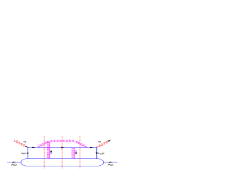
FIG. 11.:

There are three cuts in Fig. 11 and we have

$$\overline{H}^{D}_{Ap-8}(y^{-},y_{1}^{-},y_{2}^{-},k_{T},x,p,q,z) = \int d\ell_{T}^{2}\frac{\vec{\ell_{T}}\cdot(\vec{\ell_{T}}-\vec{k_{T}})}{\ell_{T}^{2}(\vec{\ell_{T}}-\vec{k_{T}})^{2}}\,\frac{\alpha_{s}}{2\pi}\,\frac{C_{A}}{2}\frac{1+z^{2}}{1-z}$$ (124)

$$\times \frac{2\pi\alpha_{s}}{N_{c}}\overline{I}_{Ap-8}(y^{-},y_{1}^{-},y_{2}^{-},\ell_{T},k_{T},x,p,q,z)\,,$$ (125)

$$\overline{I}_{Ap-8,C}(y^{-},y_{1}^{-},y_{2}^{-},\ell_{T},k_{T},x,p,q,z) = -e^{i(x+x_{L})p^{+}y^{-}+ix_{D}p^{+}(y_{1}^{-}-y_{2}^{-})}\theta(-y_{2}^{-})\theta(y^{-}-y_{1}^{-})$$ (126)

$$\times [e^{ix_{D}p^{+}y_{2}^{-}/(1-z)}-e^{-ix_{L}p^{+}y_{2}^{-}}]$$ (127)

$$\times [1-e^{-ix_{L}p^{+}(y^{-}-y_{1}^{-})}]\,,$$ (128)

$$\overline{I}_{Ap-8,L}(y^{-},y_{1}^{-},y_{2}^{-},\ell_{T},k_{T},x,p,q,z) = -e^{i(x+x_{L})p^{+}y^{-}+ix_{D}p^{+}(y_{1}^{-}-y_{2}^{-})}\theta(y^{-}-y_{1}^{-})\theta(y_{1}^{-}-y_{2}^{-})$$ (129)

$$\times e^{-i(1-z/(1-z))x_{D}p^{+}(y_{1}^{-}-y_{2}^{-})}$$ (130)

$$\times [e^{-ix_{L}p^{+}(y^{-}-y_{1}^{-})}-e^{ix_{D}p^{+}(y^{-}-y_{1}^{-})/(1-z)}]\,,$$ (131)

$$\overline{I}_{Ap-8,R}(y^{-},y_{1}^{-},y_{2}^{-},\ell_{T},k_{T},x,p,q,z) = -e^{i(x+x_{L})p^{+}y^{-}+ix_{D}p^{+}(y_{1}^{-}-y_{2}^{-})}\theta(-y_{2}^{-})\theta(y_{2}^{-}-y_{1}^{-})$$ (132)

$$\times [e^{-ix_{L}p^{+}y_{2}^{-}}-e^{ix_{D}p^{+}y_{2}^{-}/(1-z)}]\,,$$ (133)

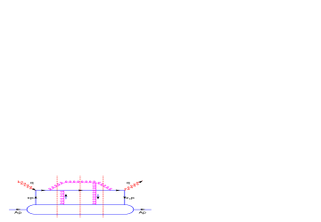
FIG. 12.:

The contributions from the three cuts in Fig. 12 can be read as

$$\overline{H}^{D}_{Ap-9}(y^{-},y_{1}^{-},y_{2}^{-},k_{T},x,p,q,z) = \int d\ell_{T}^{2}\frac{\vec{\ell_{T}}\cdot(\vec{\ell_{T}}-\vec{k_{T}})}{\ell_{T}^{2}(\vec{\ell_{T}}-\vec{k_{T}})^{2}}\,\frac{\alpha_{s}}{2\pi}\,\frac{C_{A}}{2}\frac{1+z^{2}}{1-z}$$ (134)

$$\times \frac{2\pi\alpha_{s}}{N_{c}}\overline{I}_{Ap-9}(y^{-},y_{1}^{-},y_{2}^{-},\ell_{T},k_{T},x,p,q,z)\,,$$ (135)

$$\overline{I}_{Ap-9,C}(y^{-},y_{1}^{-},y_{2}^{-},\ell_{T},k_{T},x,p,q,z) = -e^{i(x+x_{L})p^{+}y^{-}+ix_{D}p^{+}(y_{1}^{-}-y_{2}^{-})}\theta(-y_{2}^{-})\theta(y^{-}-y_{1}^{-})$$ (136)

$$\times [e^{ix_{D}p^{+}(y^{-}-y_{1}^{-})/(1-z)}-e^{-ix_{L}p^{+}(y^{-}-y_{1}^{-})}]$$ (137)

$$\times [1-e^{-ix_{L}p^{+}y_{2}^{-}}]\,,$$ (138)

$$\overline{I}_{Ap-9,L}(y^{-},y_{1}^{-},y_{2}^{-},\ell_{T},k_{T},x,p,q,z) = -e^{i(x+x_{L})p^{+}y^{-}+ix_{D}p^{+}(y_{1}^{-}-y_{2}^{-})}\theta(y^{-}-y_{1}^{-})\theta(y_{1}^{-}-y_{2}^{-})$$ (139)

$$\times [e^{-ix_{L}p^{+}(y^{-}-y_{1}^{-})}-e^{ix_{D}p^{+}(y^{-}-y_{1}^{-})/(1-z)}]\,,$$ (140)

$$\overline{I}_{Ap-9,R}(y^{-},y_{1}^{-},y_{2}^{-},\ell_{T},k_{T},x,p,q,z) = -e^{i(x+x_{L})p^{+}y^{-}+ix_{D}p^{+}(y_{1}^{-}-y_{2}^{-})}\theta(-y_{2}^{-})\theta(y_{2}^{-}-y_{1}^{-})$$ (141)

$$\times e^{-i(1-z/(1-z))x_{D}p^{+}(y_{1}^{-}-y_{2}^{-})}$$ (142)

$$\times [e^{-ix_{L}p^{+}y_{2}^{-}}-e^{ix_{D}p^{+}y_{2}^{-}/(1-z)}]\,,$$ (143)

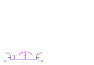
FIG. 13.:

In Fig. 13 there are two possible cuts (central or left). We have

$$\overline{H}^{D}_{Ap-10,C}(y^{-},y_{1}^{-},y_{2}^{-},k_{T},x,p,q,z) = \int d\ell_{T}^{2}\frac{(\vec{\ell_{T}}-\vec{k_{T}})\cdot(\vec{\ell_{T}}-(1-z)\vec{k_{T}})}{(\vec{\ell_{T}}-\vec{k_{T}})^{2}(\vec{\ell_{T}}-(1-z)\vec{k_{T}})^{2}}\,\frac{\alpha_{s}}{2\pi}\,\frac{C_{A}}{2}\frac{1+z^{2}}{1-z}$$ (144)

$$\times \frac{2\pi\alpha_{s}}{N_{c}}\overline{I}_{Ap-10,C}(y^{-},y_{1}^{-},y_{2}^{-},\ell_{T},k_{T},x,p,q,z)\,,$$ (145)

$$\overline{I}_{Ap-10,C}(y^{-},y_{1}^{-},y_{2}^{-},\ell_{T},k_{T},x,p,q,z) = e^{i(x+x_{L})p^{+}y^{-}+ix_{D}p^{+}(y_{1}^{-}-y_{2}^{-})}\,\theta(-y_{2}^{-})\theta(y^{-}-y_{1}^{-})$$ (146)

$$\times e^{-ix_{L}p^{+}y_{2}^{-}}[e^{ix_{D}p^{+}(y^{-}-y_{1}^{-})/(1-z)}-e^{-ix_{L}p^{+}(y^{-}-y_{1}^{-})}]\,,$$ (147)

$$\overline{H}^{D}_{Ap-10,R}(y^{-},y_{1}^{-},y_{2}^{-},k_{T},x,p,q,z) = \int d\ell_{T}^{2}\frac{\vec{\ell_{T}}\cdot(\vec{\ell_{T}}-z\vec{k_{T}})}{\ell_{T}^{2}(\vec{\ell_{T}}-z\vec{k_{T}})^{2}}\,\frac{\alpha_{s}}{2\pi}\,\frac{C_{A}}{2}\frac{1+z^{2}}{1-z}$$ (148)

$$\times \frac{2\pi\alpha_{s}}{N_{c}}\overline{I}_{Ap-10,R}(y^{-},y_{1}^{-},y_{2}^{-},\ell_{T},k_{T},x,p,q,z)\,,$$ (149)

$$\overline{I}_{Ap-10,R}(y^{-},y_{1}^{-},y_{2}^{-},\ell_{T},k_{T},x,p,q,z) = e^{i(x+x_{L})p^{+}y^{-}+ix_{D}p^{+}(y_{1}^{-}-y_{2}^{-})}\,\theta(-y_{2}^{-})\theta(y_{2}^{-}-y_{1}^{-})$$ (150)

$$\times [e^{-i(x_{D}-x_{D}^{0})p^{+}(y_{1}^{-}-y_{2}^{-})-ix_{L}p^{+}y_{1}^{-}}$$ (152)

$$-e^{-i(1-z/(1-z))x_{D}p^{+}(y_{1}^{-}-y_{2}^{-})-ix_{L}p^{+}y_{2}^{-}}]\,.$$

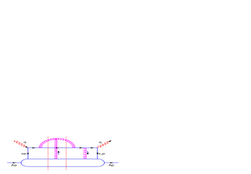
FIG. 14.:

In Fig. 14 we can make the central cut or the left cut and we obtain

$$\overline{H}^{D}_{Ap-11,C}(y^{-},y_{1}^{-},y_{2}^{-},k_{T},x,p,q,z) = \int d\ell_{T}^{2}\frac{(\vec{\ell_{T}}-\vec{k_{T}})\cdot(\vec{\ell_{T}}-(1-z)\vec{k_{T}})}{(\vec{\ell_{T}}-\vec{k_{T}})^{2}(\vec{\ell_{T}}-(1-z)\vec{k_{T}})^{2}}\,\frac{\alpha_{s}}{2\pi}\,\frac{C_{A}}{2}\frac{1+z^{2}}{1-z}$$ (153)

$$\times \frac{2\pi\alpha_{s}}{N_{c}}\overline{I}_{Ap-11,C}(y^{-},y_{1}^{-},y_{2}^{-},\ell_{T},k_{T},x,p,q,z)\,,$$ (154)

$$\overline{I}_{Ap-11,C}(y^{-},y_{1}^{-},y_{2}^{-},\ell_{T},k_{T},x,p,q,z) = e^{i(x+x_{L})p^{+}y^{-}+ix_{D}p^{+}(y_{1}^{-}-y_{2}^{-})}\,\theta(-y_{2}^{-})\theta(y^{-}-y_{1}^{-})$$ (155)

$$\times e^{-ix_{L}p^{+}(y^{-}-y_{1}^{-})}[e^{ix_{D}p^{+}y_{2}^{-}/(1-z)}-e^{-ix_{L}p^{+}y_{2}^{-}}]\,,$$ (156)

$$\overline{H}^{D}_{Ap-11,R}(y^{-},y_{1}^{-},y_{2}^{-},k_{T},x,p,q,z) = \int d\ell_{T}^{2}\frac{\vec{\ell_{T}}\cdot(\vec{\ell_{T}}-z\vec{k_{T}})}{\ell_{T}^{2}(\vec{\ell_{T}}-z\vec{k_{T}})^{2}}\,\frac{\alpha_{s}}{2\pi}\,\frac{C_{A}}{2}\frac{1+z^{2}}{1-z}$$ (157)

$$\times \frac{2\pi\alpha_{s}}{N_{c}}\overline{I}_{Ap-11,L}(y^{-},y_{1}^{-},y_{2}^{-},\ell_{T},k_{T},x,p,q,z)\,,$$ (158)

$$\overline{I}_{Ap-11,L}(y^{-},y_{1}^{-},y_{2}^{-},\ell_{T},k_{T},x,p,q,z) = e^{i(x+x_{L})p^{+}y^{-}+ix_{D}p^{+}(y_{1}^{-}-y_{2}^{-})}\,\theta(y^{-}-y_{1}^{-})\theta(y_{1}^{-}-y_{2}^{-})$$ (159)

$$\times [e^{-i(x_{D}-x_{D}^{0})p^{+}(y_{1}^{-}-y_{2}^{-})-ix_{L}p^{+}(y^{-}-y_{2}^{-})}$$ (161)

$$-e^{-i(1-z/(1-z))x_{D}p^{+}(y_{1}^{-}-y_{2}^{-})-ix_{L}p^{+}(y^{-}-y_{1}^{-})}]\,.$$

REFERENCES

[1] M. Gyulassy and M. Plümer, Phys. Lett. B243, 432 (1990).
[2]X.-N. Wang and M. Gyulassy, Phys. Rev. Lett. 68, 1480 (1992).
[3]
X. N. Wang, Z. Huang and I. Sarcevic,
Phys. Rev. Lett. 77, 231 (1996)
[arXiv:hep-ph/9605213];
X. N. Wang and Z. Huang,
Phys. Rev. C 55, 3047 (1997)
[arXiv:hep-ph/9701227].
[4]C. A. Salgado and U. A. Wiedemann,
Phys. Rev. Lett. 89, 092303 (2002)
[arXiv:hep-ph/0204221].
[5]M. Gyulassy and X.-N. Wang, Nucl. Phys. B420, 583 (1994)
[arXiv:nucl-th/9306003];
X.-N. Wang, M. Gyulassy and M. Plümer, Phys. Rev. D 51, 3436 (1995)
[arXiv:hep-ph/9408344].
[6] R. Baier et al., Nucl. Phys. B483, 291 (1997)
[arXiv:hep-ph/9607355];
Nucl. Phys. B484, 265 (1997)
[arXiv:hep-ph/9608322];
Phys. Rev. C 58, 1706 (1998)
[arXiv:hep-ph/9803473].
[7]B. G. Zhakharov, JETP letters 63, 952 (1996)
[arXiv:hep-ph/9607440].
[8] M. Gyulassy, P. Lévai and I. Vitev, Nucl. Phys.
B594, 371 (2001)
[arXiv:nucl-th/0006010];
Phys. Rev. Lett. 85, 5535 (2000)
[arXiv:nucl-th/0005032].
[10]
K. Adcox et al. [PHENIX Collaboration],
Phys. Rev. Lett. 88, 022301 (2002)
[arXiv:nucl-ex/0109003].
[11]
C. Adler et al. [STAR Collaboration],
Phys. Rev. Lett. 89, 202301 (2002)
[arXiv:nucl-ex/0206011].
[12]
E. Wang and X.-N. Wang,
Phys. Rev. Lett. 89, 162301 (2002)
[arXiv:hep-ph/0202105].
[13] X.-N. Wang and X. F. Guo,
Nucl. Phys. A 696, 788 (2001)
[arXiv:hep-ph/0102230];
X. F. Guo and X.-N. Wang,
Phys. Rev. Lett. 85, 3591 (2000)
[arXiv:hep-ph/0005044].
[14]
M. Luo, J. Qiu and G. Sterman, Phys. Lett. B279, 377 (1992);
M. Luo, J. Qiu and G. Sterman, Phys. Rev. D50, 1951 (1994);
M. Luo, J. Qiu and G. Sterman, Phys. Rev. D49, 4493 (1994).
[15]L. D. Landau and I. J. Pomeranchuk, Dolk. Akad. Nauk.
SSSR 92, 92(1953); A. B. Migdal, Phys. Rev. 103,
1811 (1956).
[16]V. N. Gribov and L. N. Lipatov, Sov. J. Nucl. Phys. 15,
438 (1972); Yu. L. Dokshitzer, Sov. Phys. JETP 46, 641 (1977);
G. Altarelli and G. Parisi, Nucl. Phys. B126, 298 (1977);
[17] J. Osborne and X.-N. Wang,
Nucl. Phys. A 710, 281 (2002)
[arXiv:hep-ph/0204046].
[18] A. H. Mueller and J. Qiu, Nucl. Phys. B268, 427 (1986).