KA-TP-2-2003
MPI-PhT/2003-03
PSI-PR-03-03
LC-TH-2003-008
hep-ph/0301189

Electroweak radiative corrections to
single Higgs-boson production in ${\mathrm{e^{+}}}{\mathrm{e^{-}}}$ annihilation

A. Denner¹, S. Dittmaier², M. Roth³ and M.M. Weber¹

¹ Paul-Scherrer-Institut, Würenlingen und Villigen
CH-5232 Villigen PSI, Switzerland

² Max-Planck-Institut für Physik (Werner-Heisenberg-Institut)
D-80805 München, Germany

³ Institut für Theoretische Physik, Universität Karlsruhe
D-76128 Karslruhe, Germany

Abstract:

We have calculated the complete electroweak ${\cal O}(\alpha)$ radiative corrections to the single Higgs-boson production processes ${\mathrm{e^{+}}}{\mathrm{e^{-}}}\to\nu_{l}\bar{\nu}_{l}{\mathrm{H}}$ ($l={\mathrm{e}},\mu,\tau$) in the electroweak Standard Model. Initial-state radiation beyond ${\cal{O}}(\alpha)$ is included in the structure-function approach. The calculation of the corrections is briefly described, and numerical results are presented for the total cross section. In the $G_{\mu}$ scheme, the bulk of the corrections is due to initial-state radiation, which affects the cross section at the level of $-7\%$ at high energies and even more in the ${\mathrm{Z}}{\mathrm{H}}$ threshold region. The remaining bosonic and fermionic corrections are at the level of a few per cent. The confusing situation in the literature regarding differing results for the fermionic corrections to this process is clarified.

January 2003

1 Introduction

The investigation of the mechanism of electroweak symmetry breaking in general and of the Higgs boson in particular will be one of the main tasks at future colliders. While the LHC will discover the Higgs boson, if it exists and has no particularly exotic properties, its complete profile can only be studied in the clean environment of an electron–positron linear collider. These studies require adequate theoretical predictions including radiative corrections and finite-width effects.

In ${\mathrm{e^{+}}}{\mathrm{e^{-}}}$ annihilation there are two main production mechanisms for the Standard Model (SM) Higgs boson. The cross section of the Higgs-strahlung process, ${\mathrm{e^{+}}}{\mathrm{e^{-}}}\to{\mathrm{Z}}{\mathrm{H}}$, rises sharply at threshold to a maximum a few tens of GeV above the threshold energy $M_{\mathrm{Z}}+M_{\mathrm{H}}$ and then falls off as $s^{-1}$, where $\sqrt{s}$ is the centre-of-mass (CM) energy of the ${\mathrm{e^{+}}}{\mathrm{e^{-}}}$ system. In the W-boson fusion process, ${\mathrm{e^{+}}}{\mathrm{e^{-}}}\to\nu_{\mathrm{e}}\bar{\nu}_{\mathrm{e}}{\mathrm{H}}$, the incoming ${\mathrm{e^{+}}}$ and ${\mathrm{e^{-}}}$ each emit a virtual W boson which fuse into a Higgs boson. The corresponding cross section grows as $\ln s$ and thus is the dominant production mechanism for large energies.

In lowest order, the Higgs-strahlung process has been studied in Ref. [1] and the vector-boson fusion process in Ref. [2]. The ${\cal{O}}(\alpha)$ electroweak radiative corrections to the process ${\mathrm{e^{+}}}{\mathrm{e^{-}}}\to{\mathrm{Z}}{\mathrm{H}}$ have been calculated by different groups [3] many years ago. The electroweak corrections to ${\mathrm{e^{+}}}{\mathrm{e^{-}}}\to\nu\bar{\nu}{\mathrm{H}}$ have attracted a lot of interest recently. In Ref. [4] the leading corrections in the limit of a heavy top quark, as well as the corresponding QCD corrections in ${\cal O}(\alpha_{\mathrm{s}}^{n}G_{\mu}m_{\mathrm{t}}^{2})$ with $n=1,2$, have been worked out. The contributions of fermion and sfermion loops in the Minimal Supersymmetric Standard Model have been evaluated in Refs. [5, 6]; at first sight, however, the results of the two calculations do not agree, not even on the fermion-loop contributions in the SM. A first calculation of the complete ${\cal{O}}(\alpha)$ electroweak corrections to ${\mathrm{e^{+}}}{\mathrm{e^{-}}}\to\nu\bar{\nu}{\mathrm{H}}$ in the SM has been performed very recently [7]. Analytical results for the one-loop corrections to this process have also been obtained by another group [8] as MAPLE output, but a numerical evaluation of these results is not yet available.

In this paper we present first results of a completely independent calculation of the ${\cal{O}}(\alpha)$ electroweak corrections to the complete process ${\mathrm{e^{+}}}{\mathrm{e^{-}}}\to\nu\bar{\nu}{\mathrm{H}}$ in the SM. Details on this calculation will be given elsewhere. Here we sketch only the main ingredients.

2 Method of calculation

We have calculated the complete ${\cal{O}}(\alpha)$ electroweak virtual and real photonic corrections to the processes ${\mathrm{e^{+}}}{\mathrm{e^{-}}}\to\nu_{\mathrm{e}}\bar{\nu}_{\mathrm{e}}{\mathrm{H}}$, $\nu_{\mu}\bar{\nu}_{\mu}H$, and $\nu_{\tau}\bar{\nu}_{\tau}H$. For ${\mathrm{e^{+}}}{\mathrm{e^{-}}}\to\nu_{\mathrm{e}}\bar{\nu}_{\mathrm{e}}{\mathrm{H}}$, this includes both the corrections to the Higgs-strahlung and the vector-boson fusion processes, which are taken into account coherently.

The calculation of the one-loop diagrams has been performed in the ’t Hooft–Feynman gauge both in the conventional and in the background-field formalism using the conventions of Refs. [9] and [10], respectively. The renormalization is carried out in the on-shell renormalization scheme, as described there. The electron mass $m_{\mathrm{e}}$ is neglected whenever possible.

The calculation of the Feynman diagrams has been performed in two completely independent ways, leading to two independent computer codes for the numerical evaluation. Both calculations are based on the methods described in Ref. [9]. The tensor coefficients of the one-loop integrals are recursively reduced to scalar integrals with the Passarino–Veltman algorithm [11] at the numerical level. The scalar integrals are evaluated using the methods and results of Refs. [9, 12], where ultraviolet divergences are regulated dimensionally and IR divergences with an infinitesimal photon mass. The two calculations differ in the following points. In the first calculation, the Feynman graphs are generated with FeynArts version 1.0 [13]. Using Mathematica the amplitudes are expressed in terms of standard matrix elements and coefficients of tensor integrals. Tensor 5-point functions have been evaluated both by applying the usual Passarino–Veltman reduction and by using the direct reduction to 4-point integrals of Ref. [14]. While the results based on the Passarino–Veltman algorithm become numerically unstable at the phase-space boundary owing to the appearance of inverse Gram determinants and could only be rescued by a careful extrapolation out of the numerically safe inner phase-space domains, the direct reduction of Ref. [14] avoids inverse leading Gram determinants, rendering the results of this approach well behaved near the phase-space boundary. The whole calculation has been carried out in the conventional and in the background-field formalism. The second calculation has been done with the help of FeynArts version 3 [15] and FormCalc [16]. The analytical expressions generated by FormCalc were translated into C code. In order to eliminate 5-point tensor integrals the interference of the pentagon diagrams with the lowest-order amplitude was evaluated with FeynCalc [17] by evaluating the fermion traces. Then the loop momenta of the 5-point integrals appeared in the numerator only in scalar products which could be cancelled with denominators, leaving only scalar 5-point integrals.

The results of the two different codes, those obtained within the conventional and background-field formalism, and those resulting from different treatments of the tensor 5-point functions are all in good numerical agreement (typically within at least 12 digits for non-exceptional phase-space points).

We use two different schemes for the inclusion of the finite Z-boson decay width. In the fixed-width scheme, each resonant Z-boson propagator $1/(s_{\nu\bar{\nu}}-M_{\mathrm{Z}}^{2})$, where $s_{\nu\bar{\nu}}$ is the invariant mass of the neutrino–antineutrino pair, is replaced by $1/(s_{\nu\bar{\nu}}-M_{\mathrm{Z}}^{2}+{\mathrm{i}}M_{\mathrm{Z}}\Gamma_{{\mathrm{Z}}})$, while non-resonant contributions are kept untouched. As a second option, we applied a factorization scheme where the full (gauge-invariant) ${\mathrm{Z}}{\mathrm{H}}$-production amplitude with zero ${\mathrm{Z}}$-boson width is rescaled by a factor $(s_{\nu\bar{\nu}}-M_{\mathrm{Z}}^{2})/(s_{\nu\bar{\nu}}-M_{\mathrm{Z}}^{2}+{\mathrm{i}}M_{\mathrm{Z}}\Gamma_{{\mathrm{Z}}})$. Within integration errors both schemes give the same results for the total cross section.

The matrix elements for the real photonic corrections are evaluated using the Weyl–van der Waerden spinor technique as formulated in Ref. [18] and have been successfully checked against the result obtained with the package Madgraph [19]. The soft and collinear singularities are treated both in the dipole subtraction method following Refs. [20, 21] and in the phase-space slicing method following closely Ref. [22]. Beyond ${\cal{O}}(\alpha)$ initial-state-radiation (ISR) corrections are included at the leading-logarithmic level using the structure functions given in Ref. [23] (for the original papers see references therein).

The phase-space integration is performed with Monte Carlo techniques in both computer codes. The first code employs a multi-channel Monte Carlo generator similar to the one implemented in RacoonWW [21, 24] and Lusifer [25], the second one uses the adaptive multi-dimensional integration program VEGAS [26].

3 Numerical results

3.1 Input parameters

For the numerical evaluation we use the following set of SM parameters [27],

$$\begin{array}[b]{lcllcllcl}G_{\mu}&=&1.16639\times 10^{-5}\,\mathrm{GeV}^{-2},&\alpha(0)&=&1/137.03599976,\\ M_{\mathrm{W}}&=&80.423\,\mathrm{GeV},&M_{\mathrm{Z}}^{\mathrm{LEP}}&=&91.1876\,\mathrm{GeV},&\Gamma_{{\mathrm{Z}}}^{\mathrm{LEP}}&=&2.4952\,\mathrm{GeV},\\ m_{\mathrm{e}}&=&0.510998902\,\mathrm{MeV},&m_{\mu}&=&105.658357\,\mathrm{MeV},&m_{\tau}&=&1.77699\,\mathrm{GeV},\\ m_{\mathrm{u}}&=&66\,\mathrm{MeV},&m_{\mathrm{c}}&=&1.2\,\mathrm{GeV},&m_{\mathrm{t}}&=&174.3\;\,\mathrm{GeV},\\ m_{\mathrm{d}}&=&66\,\mathrm{MeV},&m_{\mathrm{s}}&=&150\,\mathrm{MeV},&m_{\mathrm{b}}&=&4.3\,\mathrm{GeV}.\end{array}$$ (3.1)

We do not calculate the W-boson mass from $G_{\mu}$ but use its experimental value as input. Since we employ a fixed width in the resonant Z-boson propagator in contrast to the approach used at LEP to fit the Z resonance, where a running width is taken, we have to convert the “on-shell” values of $M_{\mathrm{Z}}^{\mathrm{LEP}}$ and $\Gamma_{{\mathrm{Z}}}^{\mathrm{LEP}}$, resulting from LEP, to the “pole values” denoted by $M_{\mathrm{Z}}$ and $\Gamma_{{\mathrm{Z}}}$ in this paper. The relation of the two sets of values is given by [28]

$$M_{\mathrm{Z}} = M_{\mathrm{Z}}^{\mathrm{LEP}}/\sqrt{1+(\Gamma_{{\mathrm{Z}}}^{\mathrm{LEP}}/M_{\mathrm{Z}}^{\mathrm{LEP}})^{2}}=91.1535\,\mathrm{GeV},$$

$$\Gamma_{{\mathrm{Z}}} = \Gamma_{{\mathrm{Z}}}^{\mathrm{LEP}}/\sqrt{1+(\Gamma_{{\mathrm{Z}}}^{\mathrm{LEP}}/M_{\mathrm{Z}}^{\mathrm{LEP}})^{2}}=2.4943\,\mathrm{GeV},$$ (3.2)

i.e. the difference is of formal two-loop order and numerically hardly visible in the results presented below. The masses of the light quarks are adjusted to reproduce the hadronic contribution to the photonic vacuum polarization of Ref. [29]. Since we parametrize the lowest-order cross section with the Fermi constant $G_{\mu}$ ($G_{\mu}$ scheme), i.e. we derive the electromagnetic coupling $\alpha$ according to $\alpha_{G_{\mu}}=\sqrt{2}G_{\mu}M_{\mathrm{W}}^{2}s_{\mathrm{w}}^{2}/\pi$, the results are practically independent of the masses of the light quarks. Moreover, this procedure absorbs the corrections proportional to $m_{\mathrm{t}}^{2}/M_{\mathrm{W}}^{2}$ in the fermion–W-boson couplings and the running of $\alpha(Q^{2})$ from $Q^{2}=0$ to the electroweak scale. In the relative radiative corrections, we use, however, $\alpha(0)$ as coupling parameter, which is the correct effective coupling for real photon emission.

We always sum over all three neutrino species, i.e. over the processes ${\mathrm{e^{+}}}{\mathrm{e^{-}}}\to\nu_{\mathrm{e}}\bar{\nu}_{\mathrm{e}}{\mathrm{H}}$, $\nu_{\mu}\bar{\nu}_{\mu}H$, and $\nu_{\tau}\bar{\nu}_{\tau}H$. Besides the full cross section, denoted “total” in the plots, we also give the cross section resulting from the ${\mathrm{Z}}{\mathrm{H}}$-production channel and the ${\mathrm{W}}{\mathrm{W}}$-fusion channel separately, which are referred to as “ZH” and “WW” contributions, respectively. In the ${\mathrm{Z}}{\mathrm{H}}$-production channel we sum over the relevant contributions of all $\nu\bar{\nu}{\mathrm{H}}$ final states, which is equivalent to multiplying the cross sections for ${\mathrm{e^{+}}}{\mathrm{e^{-}}}\to\nu_{\mu}\bar{\nu}_{\mu}{\mathrm{H}}$ by a factor 3. This means that the results shown for “total” and “ZH+WW” only differ by the interference terms between the ${\mathrm{Z}}{\mathrm{H}}$ and ${\mathrm{W}}{\mathrm{W}}$ channels. In the results presented here, the ISR is convoluted only with the lowest-order cross section. We consider merely total cross sections without any cuts; distributions will be discussed elsewhere.

For reference we give some numbers for the total cross section in lowest order, $\sigma_{\mathrm{tree}}$, and including electroweak corrections, $\sigma$, together with the relative corrections defined as $\delta=\sigma/\sigma_{\mathrm{tree}}-1$ in Table 1.

$M_{\mathrm{H}}$ [GeV]	$\sigma_{\mathrm{tree}}$ [fb]	$\sigma$ [fb]	$\delta$ [%]
115	92.64(2)	85.01(8)	$~{}{-8.2(1)}$
150	68.17(2)	61.76(5)	$~{}{-9.4(1)}$
200	41.800(9)	37.76(3)	$~{}{-9.7(1)}$
250	23.764(4)	20.97(1)	${-11.8(1)}$
300	12.125(2)	10.478(6)	${-13.6(1)}$
350	5.2047(6)	4.264(2)	${-18.1(1)}$

Table 1: Lowest-order cross section for ${\mathrm{e^{+}}}{\mathrm{e^{-}}}\to\nu\bar{\nu}{\mathrm{H}}$ in the $G_{\mu}$-scheme, $\sigma_{\mathrm{tree}}$, cross section including full electroweak corrections, $\sigma$, and relative corrections $\delta$ for various Higgs masses at $\sqrt{s}=500\,\mathrm{GeV}$

The last numbers in parentheses correspond to the Monte Carlo integration error of the last given digit.

In Figure 1 we show the lowest-order cross section as a function of the CM energy for $M_{\mathrm{H}}=115\,\mathrm{GeV}$ and $150\,\mathrm{GeV}$. Besides the total contribution we separately give also the contributions from ${\mathrm{Z}}{\mathrm{H}}$ production and ${\mathrm{W}}{\mathrm{W}}$ fusion as defined above.

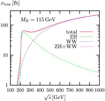
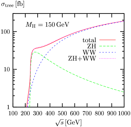
Figure 1: Lowest-order cross section and contributions from ${\mathrm{Z}}{\mathrm{H}}$-production and ${\mathrm{W}}{\mathrm{W}}$-fusion channels for $M_{\mathrm{H}}=115\,\mathrm{GeV}$ and $M_{\mathrm{H}}=150\,\mathrm{GeV}$

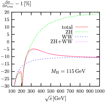
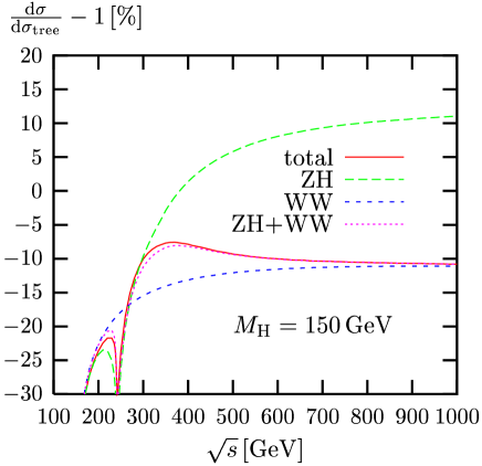
Figure 2: Relative electroweak corrections to the complete process ${\mathrm{e^{+}}}{\mathrm{e^{-}}}\to\nu\bar{\nu}{\mathrm{H}}$ and to the contributions from ${\mathrm{Z}}{\mathrm{H}}$-production and ${\mathrm{W}}{\mathrm{W}}$-fusion channels for $M_{\mathrm{H}}=115\,\mathrm{GeV}$ and $M_{\mathrm{H}}=150\,\mathrm{GeV}$

Below the ${\mathrm{Z}}{\mathrm{H}}$ threshold and above $400\,\mathrm{GeV}$ the cross section is dominated by ${\mathrm{W}}{\mathrm{W}}$ fusion. The ${\mathrm{Z}}{\mathrm{H}}$-production contribution dominates from the ${\mathrm{Z}}{\mathrm{H}}$ threshold up to about $300\,\mathrm{GeV}$. Comparing the “total” cross section with the sum “ZH+WW”, one can see that the interference contributions between ${\mathrm{Z}}{\mathrm{H}}$ and ${\mathrm{W}}{\mathrm{W}}$ channels are small in lowest order for the inspected kinematical situation.

The relative corrections to the lowest-order contributions of Figure 1 are shown in Figure 2. The corrections to the ${\mathrm{Z}}{\mathrm{H}}$-production channel are large and negative ($\mathrel{\raisebox{-3.00003pt}{$\stackrel{{\scriptstyle\displaystyle<}}{{\sim}}$}}-20\%$) below threshold, rise fast above threshold, and reach 19% and 11% at $\sqrt{s}=1\,\mathrm{TeV}$ for $M_{\mathrm{H}}=115\,\mathrm{GeV}$ and $M_{\mathrm{H}}=150\,\mathrm{GeV}$, respectively. The corrections to the ${\mathrm{W}}{\mathrm{W}}$-fusion channel are similar below the ${\mathrm{Z}}{\mathrm{H}}$ threshold, rise sharply at the threshold and are flat and about $-10\%$ above $500\,\mathrm{GeV}$. The corrections to the complete process are always negative. They follow those of the ${\mathrm{Z}}{\mathrm{H}}$-production channel for energies below $\sim 300\,\mathrm{GeV}$ and those of the ${\mathrm{W}}{\mathrm{W}}$-fusion channel above $\sim 500\,\mathrm{GeV}$.

The contributions of ${\cal{O}}(\alpha)$ ISR corrections, ISR beyond ${\cal{O}}(\alpha)$, fermionic corrections, and non-ISR bosonic corrections to the ${\mathrm{Z}}{\mathrm{H}}$-production and ${\mathrm{W}}{\mathrm{W}}$-fusion channels are presented in Figure 3.

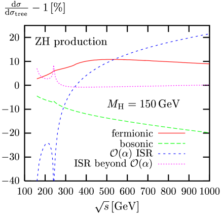
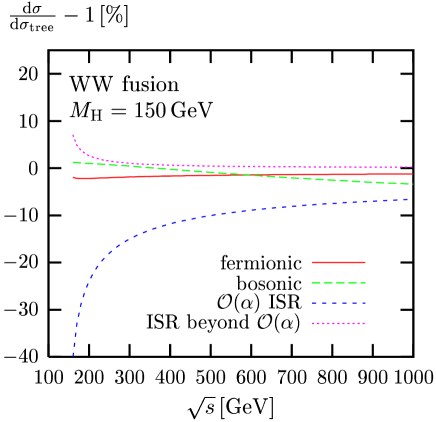
Figure 3: Relative electroweak corrections to the ${\mathrm{Z}}{\mathrm{H}}$-production (left) and ${\mathrm{W}}{\mathrm{W}}$-fusion (right) channels resulting from ${\cal{O}}(\alpha)$ ISR, ISR beyond ${\cal{O}}(\alpha)$, fermion loops, and non-ISR bosonic corrections for $M_{\mathrm{H}}=150\,\mathrm{GeV}$

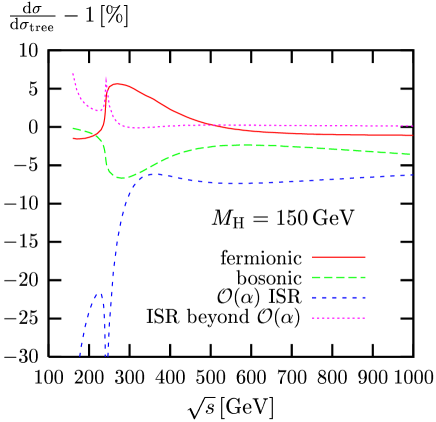
Figure 4: Relative electroweak corrections to the complete lowest-order cross sections resulting from ${\cal{O}}(\alpha)$ ISR, ISR beyond ${\cal{O}}(\alpha)$, fermion loops, and non-ISR bosonic corrections for $M_{\mathrm{H}}=150\,\mathrm{GeV}$

The ${\cal{O}}(\alpha)$ ISR corrections are defined as the ${\cal{O}}(\alpha)$ contributions of the structure functions of Ref. [23]. The fermionic corrections summarize all fermion-loop contributions to loop diagrams and counter terms. The non-ISR bosonic corrections are obtained by subtracting the ${\cal{O}}(\alpha)$ ISR corrections and the fermionic corrections from the complete ${\cal{O}}(\alpha)$ corrections. It can be seen, that the energy dependence in both channels and, in particular, the rise of the corrections to the ${\mathrm{Z}}{\mathrm{H}}$-production channel with energy is essentially due to the ISR corrections. The large corrections above the peak of the lowest-order ${\mathrm{Z}}{\mathrm{H}}$ cross section are due to the decreasing cross section. Since the ISR corrections increase with the height of this peak, they are larger for smaller Higgs masses (see Figure 2). The ISR corrections beyond ${\cal{O}}(\alpha)$ are at the level of several per cent where the lowest-order cross section rises strongly, but are below 1% above $300\,\mathrm{GeV}$. The non-ISR corrections provide a measure of the genuinely weak corrections. For the ${\mathrm{Z}}{\mathrm{H}}$-production channel (Figure 3 left) the fermionic corrections increase slowly from 3% to 11% around $500\,\mathrm{GeV}$ and then go down to $9\%$ at $1\,\mathrm{TeV}$. The non-ISR bosonic corrections decrease from $-5\%$ to $-20\%$ over the considered energy range. This behaviour is typical if electroweak Sudakov logarithms of the form $-\alpha\ln^{2}(s/M_{\mathrm{Z}}^{2})$ dominate the corrections, which is always the case if the major part of the total cross section results from intermediate scattering angles. For the ${\mathrm{W}}{\mathrm{W}}$-fusion channel (Figure 3 right), the ISR corrections are negative for all energies, which can be explained by the rising cross section with increasing scattering energy. ISR beyond ${\cal{O}}(\alpha)$ influences the cross section only at the level of $\mathrel{\raisebox{-3.00003pt}{$\stackrel{{\scriptstyle\displaystyle<}}{{\sim}}$}}1\%$ for energies above $300\,\mathrm{GeV}$. The fermionic corrections are between $-1\%$ and $-2\%$ over the whole energy range. The non-ISR bosonic corrections fall from $+1\%$ at threshold to $-3\%$ at $\sqrt{s}=1\,\mathrm{TeV}$. This energy dependence is much weaker than for the ${\mathrm{Z}}{\mathrm{H}}$ channel, since the cross section for the ${\mathrm{W}}{\mathrm{W}}$ channel is more and more dominated by small scattering angles, i.e. not by the Sudakov regime.

The various contributions of the corrections to the complete process are depicted in Figure 4. The size of the corrections can be easily explained by the results of Figure 3; it is given by the size of the corrections of the dominating channel. The ISR corrections vary strongly in the region of the ${\mathrm{Z}}{\mathrm{H}}$ threshold but are nearly flat and about $-7\%$ for energies above $400\,\mathrm{GeV}$. They are always negative since the lowest-order cross section is continuously rising. The fermionic corrections reach a maximum of about $6\%$ in the region where the ${\mathrm{Z}}{\mathrm{H}}$-production channel dominates and are between $0\%$ and $-1\%$ above $500\,\mathrm{GeV}$ where the ${\mathrm{W}}{\mathrm{W}}$-fusion process dominates. The non-ISR bosonic corrections exhibit a minimum of about $-7\%$ where the ${\mathrm{Z}}{\mathrm{H}}$-production channel dominates and are between $0\%$ and $-4\%$ elsewhere.

4 Comparison with other calculations

We have compared our results for the ${\cal{O}}(\alpha)$ corrections to Ref. [7] and the contributions from closed fermion loops with Refs. [5, 6].

Adapting the input parameters and the parametrization of the lowest-order matrix element to those used in Ref. [7], we reproduced the numbers in Table 2 for the total cross section given in the first paper of Ref. [7]. We find agreement within 0.2% for the total lowest-order cross section and within 0.3% for the corrected cross section. The corrections relative to the lowest-order cross section agree within 0.2%. Note that the authors of Ref. [7] use $\alpha(0)$ to parametrize the lowest-order cross section. As a consequence their relative corrections are shifted by $3\Delta r\approx+9\%$ compared to those in the $G_{\mu}$ scheme.

Adapting the input parameters to those of Ref. [6], who also use the $G_{\mu}$ scheme, we perfectly reproduce the SM results of these authors for the tree-level cross section and the fermionic corrections.

The authors of Ref. [5] use $\hat{\alpha}(M_{\mathrm{Z}})$, i.e. the running electromagnetic coupling in the $\overline{\mathrm{MS}}$ scheme at $M_{\mathrm{Z}}$, as defined in Eq. (B.2) of Ref. [30], to parametrize the lowest-order cross section. The relative fermionic corrections in this scheme differ from those in the $G_{\mu}$ scheme by $3[(\Delta r)_{\mathrm{ferm}}-\Delta\hat{\alpha}(M_{\mathrm{Z}})]\approx-13\%$. Moreover, Eberl et al. take into account only the loops from the top–bottom doublet and omit the corrections to the ${\mathrm{Z}}{\mathrm{H}}$-production channel. Adapting to this setup, we find agreement with the results of Ref. [5] at $1\,\mathrm{TeV}$ within the integration errors for the lowest-order cross section. The corrections relative to the lowest-order cross section agree typically within 0.3%. The large differences in relative corrections between Refs. [5] and [6] thus result essentially from the use of different parametrizations of the lowest-order matrix element. The fact that the lowest-order SM cross sections in Refs. [5] and [6] agree qualitatively despite of the different input-parameter schemes used is accidental and due to the (different) input parameters.

Where the WW-fusion channel dominates, the non-ISR, i.e. the genuine weak, corrections are large if $\alpha(0)$ or $\alpha(M_{\mathrm{Z}})$ are used to parametrize the lowest-order cross section. Only when using $G_{\mu}$ the large corrections associated with the running of $\alpha$ and those proportional to $m_{\mathrm{t}}^{2}$ in the W-boson–fermion couplings are absorbed in the lowest-order cross section. For the ZH-production channel the situation is more complicated and a dedicated improved Born approximation is under investigation. It should be noted that higher-loop corrections become relevant in schemes where the one-loop corrections are large. Since ISR corrections, the running of $\alpha$, and the $m_{\mathrm{t}}$-dependent corrections are independent, one has to deal with all these terms separately.

5 Summary

We have presented results from a calculation of the complete electroweak ${\cal O}(\alpha)$ radiative corrections to the single Higgs-boson production process ${\mathrm{e^{+}}}{\mathrm{e^{-}}}\to\nu\bar{\nu}{\mathrm{H}}$ in the electroweak Standard Model. We find that the ISR corrections are of the order of $-7\%$ at high energies and more than $-10\%$ near the ${\mathrm{Z}}{\mathrm{H}}$ threshold. In this region even the higher-order ISR corrections reach several per cent. This is due to the strong energy dependence of the lowest-order cross section. The non-ISR corrections are at the level of a few per cent if the lowest order matrix element is parametrized with the Fermi constant $G_{\mu}$. In other schemes these corrections are of the order of 10%. It has been pointed out that the confusion in the literature regarding the size of the corrections to ${\mathrm{e^{+}}}{\mathrm{e^{-}}}\to\nu\bar{\nu}{\mathrm{H}}$ is due to the use of different schemes and input parameters.

References

-
[1]
J. R. Ellis, M. K. Gaillard and D. V. Nanopoulos,
Nucl. Phys. B 106 (1976) 292;
B. L. Ioffe and V. A. Khoze, Sov. J. Part. Nucl. 9 (1978) 50 [Fiz. Elem. Chast. Atom. Yadra 9 (1978) 118];
J. D. Bjorken, in Weak Interactions At High-Energy And The Production Of New Particles: Proceedings of the 4th Slac Summer Institute On Particle Physics, ed. M. C. Zipf, SLAC-198, Stanford, Calif., SLAC (1976) p. 1. -
[2]
D. R. Jones and S. T. Petcov,
Phys. Lett. B 84 (1979) 440;
G. Altarelli, B. Mele and F. Pitolli, Nucl. Phys. B 287 (1987) 205;
W. Kilian, M. Krämer and P. M. Zerwas, Phys. Lett. B 373 (1996) 135 [hep-ph/9512355];
E. Boos, M. Sachwitz, H. J. Schreiber and S. Shichanin, Int. J. Mod. Phys. A 10 (1995) 2067. -
[3]
J. Fleischer and F. Jegerlehner,
Nucl. Phys. B 216 (1983) 469;
B. A. Kniehl, Z. Phys. C 55 (1992) 605;
A. Denner, J. Küblbeck, R. Mertig and M. Böhm, Z. Phys. C 56 (1992) 261. - [4] B. A. Kniehl and M. Steinhauser, Nucl. Phys. B 454 (1995) 485 [hep-ph/9508241].
- [5] H. Eberl, W. Majerotto and V. C. Spanos, Phys. Lett. B 538 (2002) 353 [hep-ph/0204280]; hep-ph/0210038. hep-ph/0210330.
- [6] T. Hahn, S. Heinemeyer and G. Weiglein, hep-ph/0211204; hep-ph/0211384.
- [7] G. Belanger, F. Boudjema, J. Fujimoto, T. Ishikawa, T. Kaneko, K. Kato and Y. Shimizu, hep-ph/0211268; hep-ph/0212261.
- [8] F. Jegerlehner and O. Tarasov, hep-ph/0212004.
- [9] A. Denner, Fortsch. Phys. 41 (1993) 307.
- [10] A. Denner, S. Dittmaier and G. Weiglein, Nucl. Phys. B 440 (1995) 95 [hep-ph/9410338].
- [11] G. Passarino and M. Veltman, Nucl. Phys. B 160 (1979) 151.
-
[12]
G. ’t Hooft and M. Veltman,
Nucl. Phys. B 153 (1979) 365;
W. Beenakker and A. Denner, Nucl. Phys. B 338 (1990) 349. -
[13]
J. Küblbeck, M. Böhm and A. Denner,
Comput. Phys. Commun. 60 (1990) 165;
H. Eck and J. Küblbeck, Guide to FeynArts 1.0, University of Würzburg, 1992. - [14] A. Denner and S. Dittmaier, hep-ph/0212259.
- [15] T. Hahn, Comput. Phys. Commun. 140 (2001) 418 [hep-ph/0012260].
-
[16]
T. Hahn and M. Perez-Victoria,
Comput. Phys. Commun. 118 (1999) 153
[hep-ph/9807565];
T. Hahn, Nucl. Phys. Proc. Suppl. 89 (2000) 231 [hep-ph/0005029]. - [17] R. Mertig, M. Böhm and A. Denner, Comput. Phys. Commun. 64 (1991) 345.
- [18] S. Dittmaier, Phys. Rev. D 59 (1999) 016007 [hep-ph/9805445].
-
[19]
T. Stelzer and W. F. Long,
Comput. Phys. Commun. 81 (1994) 357
[hep-ph/9401258];
H. Murayama, I. Watanabe and K. Hagiwara, KEK-91-11. - [20] S. Dittmaier, Nucl. Phys. B 565 (2000) 69 [hep-ph/9904440].
- [21] M. Roth, PhD thesis, ETH Zürich No. 13363 (1999), hep-ph/0008033.
- [22] M. Böhm and S. Dittmaier, Nucl. Phys. B409 (1993) 3 and B412 (1994) 39.
- [23] W. Beenakker et al., in Physics at LEP2 (Report CERN 96-01, Geneva, 1996), G. Altarelli, T. Sjöstrand and F. Zwirner (eds.), Vol. 1, p. 79, hep-ph/9602351.
- [24] A. Denner, S. Dittmaier, M. Roth and D. Wackeroth, Nucl. Phys. B 560 (1999) 33 [hep-ph/9904472].
- [25] S. Dittmaier and M. Roth, Nucl. Phys. B 642 (2002) 307 [hep-ph/0206070].
- [26] G. P. Lepage, J. Comput. Phys. 27 (1978) 192 and CLNS-80/447.
- [27] K. Hagiwara et al. [Particle Data Group Collaboration], Phys. Rev. D 66 (2002) 010001.
-
[28]
D. Y. Bardin, A. Leike, T. Riemann and M. Sachwitz,
Phys. Lett. B 206 (1988) 539;
A. Sirlin, Phys. Rev. Lett. 67 (1991) 2127;
D. Wackeroth and W. Hollik, Phys. Rev. D 55 (1997) 6788 [hep-ph/9606398];
W. Beenakker et al., Nucl. Phys. B 500 (1997) 255 [hep-ph/9612260]. - [29] F. Jegerlehner, DESY 01-029, LC-TH-2001-035, hep-ph/0105283.
- [30] H. Eberl, M. Kincel, W. Majerotto and Y. Yamada, Nucl. Phys. B 625 (2002) 372 [hep-ph/0111303].