x $1/N_{c}$ corrections to the $SU(4)_{c}$ symmetry for $L=1$ baryons:
The Three Towers

Abstract

In the large $N_{c}$ limit, the mass spectrum of the $L=1$ orbitally excited baryons $N^{*}$ has a very simple structure, with states degenerate in pairs of spins $J=(\frac{1}{2},\frac{3}{2}),(\frac{3}{2},\frac{5}{2})$, corresponding to irreducible representations (towers) of the contracted $SU(4)_{c}$ symmetry group. The mixing angles are completely determined in this limit. Using a mass operator approach, we study $1/N_{c}$ corrections to this picture, pointing out a four-fold ambiguity in the correspondence of the observed baryons with the large $N_{c}$ states. For each of the four possible assignments, we fit the coefficients of the quark operators contributing to the mass spectrum to $O(N_{c}^{-1})$. We comment on the implications of our results for the constituent quark model description of these states.

I Introduction

Ever since their discovery, the negative-parity excited baryons have been a testing ground for the quark model, as their complex mass spectrum makes it possible to distinguish among different models of quark-quark interactions. In the quark model, the $L=1$ negative parity baryons fall into the ${\bf 70}$ representation of $SU(6)$, which contains the $({\bf 1},2)$, $({\bf 10},2)$, $({\bf 8},2)$ and $({\bf 8},4)$ of $SU(3)_{\rm fl}\otimes SU(2)_{\rm sp}$ su6 ; mix . The finer details of the spectrum were first studied in a constituent quark model by Isgur and Karl IsgKa ; CaIsg . Recently, the flavor dependence of the quark spin interactions has been a matter of some debate, related to their dynamical origin as arising from constituent gluons or pions exchange OPE ; HG ; Riska .

In this paper we focus on a different, model-independent description of these states, which was proposed only relatively recently DJM1 ; DJM2 ; CGKM ; JG ; PY1 ; PY2 ; CCGL1 ; CCGL ; CC ; SGS ; su3prd . This is based on the large $N_{c}$ limit 1 ; 2 , and makes use of the contracted $SU(2N_{f})$ symmetry of QCD in this limit DJM2 . There are two equivalent ways of extracting the predictions of this symmetry. The first method is algebraic, and makes use of commutation relations of operators representing physical quantities such as axial currents and hadron masses, which are constrained by so-called consistency conditions. Although somewhat cumbersome and difficult to extend beyond the leading order in $1/N_{c}$, such an approach has been applied to the study of the mass spectrum and strong decays of the excited light baryons in PY1 ; PY2 . These states were predicted to fall into irreducible representations of the contracted $SU(2N_{f})$ algebra, with nontrivial implications for the mass spectrum and mixing angles of the excited baryons.

A somewhat different approach to large $N_{c}$ baryons is based on the quark operators method. In this approach the representations of the contracted $SU(2N_{f})$ algebra are constructed in terms of a ‘quark’ basis $|\frac{1}{2},s_{3}\rangle\otimes|\frac{1}{2},i_{3}\rangle$. Although similar to the one-quark basis states used in the constituent quark model (CQM), we stress that this is a purely mathematical device and does not imply any of the dynamical assumptions of the CQM. Any physical quantity is further written as an expansion in $n$-body operators acting on the ‘quark’ states, ordered according to $n$. This can be organized as an expansion in $1/N_{c}$, with a finite number of independent operators contributing at any given order in $1/N_{c}$. This method for extracting the predictions of the large $N_{c}$ limit has the advantage of being more systematic and easier to extend to subleading orders in $1/N_{c}$.

The mass spectrum of the excited baryons has been studied using this approach in a series of papers CCGL1 ; CCGL ; SGS ; su3prd , including operators of order up to and including $1/N_{c}^{2}$. In these papers the coefficients of these operators have been extracted from a fit to the observed masses, yielding a very specific pattern of the dominant operators.

In this paper we reanalyze the $1/N_{c}$ expansion for the masses of the nonstrange excited baryons. Guided by the expected structure of the large $N_{c}$ mass spectrum, we present fits for the coefficients of the mass operator, order by order in $N_{c}$. We point out a four-fold ambiguity in the correspondence of the physical states with the large $N_{c}$ states, and the special status of the excited $\Delta^{*}$ states in the $N_{c}$ expansion. At leading order in $N_{c}$ only three operators contribute to the mass operator, and we discuss the four equivalent fits to their coefficients, one of which turns out to be ruled out. Including $1/N_{c}$ corrections allows eight operators to contribute to the mass matrix. Considering only data on $N^{*}$ masses, the coefficients of these eight operators can be determined as functions of the two mixing angles, up to an additional continuous ambiguity. We present restrictive constraints on the allowed set of coefficients, first from dimensional analysis and then by including data on the excited $\Delta^{*}$ states. We compare the results of our fits to those previously discussed in the literature.

II Formalism

The spin-flavor structure of the orbitally excited $L=1$ baryons for arbitrary $N_{c}$ can be conveniently described in terms of quark quantum numbers. The quark basis states can be labeled as $|J,I,S;m_{J},I_{3}\rangle$ where $S$ is the quarks’ spin, $I$ their isospin and $\vec{J}=\vec{S}+\vec{L}$ the total baryon spin. The spin-isospin wave function of a nonstrange $L=1$ orbitally excited baryon has mixed spin-flavor symmetry. This implies that for a given isospin $I$, the spin $S$ takes all values compatible with $|S-I|\leq 1$ except for $S=I=N_{c}/2$. The most general state $|JIS\rangle$ can be constructed by adding one excited quark to a symmetric ’core’ of quantum numbers $|S_{c}=I_{c}\rangle$, such that $\vec{S}=\vec{S}_{c}+\vec{s}$, $\vec{I}=\vec{I}_{c}+\vec{i}$ with $s=i=\frac{1}{2}$.

In the large $N_{c}$ limit the mass eigenstates obtained from this construction fall into irreducible representations of the contracted $SU(2N_{f})$ algebra DJM2 . These are infinite towers of states, labelled by an integer or half-integer $T$, and contain all possible states satisfying the condition $|J-I|\leq T$. All the states belonging to a tower are degenerate in mass, and the separation between towers is of order $O(N_{c}^{0})$ in the large $N_{c}$ limit. On the other hand, mass splittings within towers are small, and appear first at order $O(1/N_{c})$. The tower states $|JIT\rangle$ are related to the quark model states $|JIS\rangle$ by a simple recoupling relation PY1

$$|JIT\rangle=(-)^{I+1+L+J}\sum_{S}\sqrt{(2S+1)(2T+1)}\left\{\begin{array}[]{ccc}I&1&S\\ L&J&T\\ \end{array}\right\}|JIS\rangle\,.$$ (3)

This completely determines the mixing matrix of the $L=1$ excited baryons in the large $N_{c}$ limit, in the absence of configuration mixing .

The resulting mass spectrum for the nonstrange $P-$wave baryons is shown in Fig. 1(b). There are five $I=1/2$ states ($N-$type) which correspond to quark model states of spin $S=1/2,3/2$, and eight $I=3/2$ states ($\Delta-$type, not shown), corresponding to quark spin $S=1/2,3/2$ and $5/2$. This covers all the observed $N$ type states, but due to the finite value of $N_{c}=3$ in the real world, only two $I=3/2$ states are present. This will be seen to limit the predictive power of the large $N_{c}$ approach for the $\Delta-$type excited baryons.

Figure 1: The mass spectrum of the nonstrange $L=1$ orbitally excited nucleons. (a) the observed states and (b) in the large $N_{c}$ limit these states fall into three towers labelled by the quantum number $T=0,1,2$.

In the following we show how the large $N_{c}$ predictions are reproduced in the quark operators language. This will allow us to include also symmetry breaking to this picture, appearing at order $1/N_{c}$. The mass matrix of the $L=1$ baryons can be written as a sum of operators acting on the quark basis as

$$\hat{M}=\sum_{k=0}^{N_{c}}\frac{1}{N_{c}^{k-1}}C_{k}{\cal O}_{k}$$ (4)

with ${\cal O}_{k}$ a $k$-body operator. Both the coefficients $C_{k}$ and the matrix elements of the operators on baryon states $\langle{\cal O}_{k}\rangle$ have power expansions in $1/N_{c}$ with coefficients determined by nonperturbative dynamics

$$C_{k}=\sum_{n=0}^{\infty}\frac{1}{N_{c}^{n}}C_{k}^{(n)}\,,\qquad\langle{\cal O}_{k}\rangle=\sum_{n=0}\frac{1}{N_{c}^{n}}\langle{\cal O}_{k}\rangle^{(n)}\,.$$ (5)

The natural size for the coefficients $C_{k}^{(n)}$ is $\Lambda/N_{c}^{n}$, with $\Lambda\sim 500$ MeV. The basic building blocks for constructing the operators ${\cal O}_{k}$ are $s^{i},\tau^{a},g^{ia}$ (acting on the excited quark), $S_{c}^{i},G_{c}^{ia}$ (acting on the core), and operators acting on the orbital degrees of freedom $l^{i},l^{(2)ij}=\frac{1}{2}\{l^{i},l^{j}\}-\frac{1}{3}l^{2}\delta^{ij}$.

We will use the operator basis introduced in CCGL , which contains the following operators, ordered according to their leading power in $1/N_{c}$. At leading order in $N_{c}$ only three operators contribute to the mass matrix, given by

$${\cal O}_{1}=N_{c}{\bf 1}\,,\qquad{\cal O}_{2}=l^{i}s^{i}\,,\qquad{\cal O}_{3}=\frac{3}{N_{c}}l^{(2)ij}g^{ia}G_{c}^{ja}\,.$$ (6)

One small technical difference with the operators in CCGL is that we define ${\cal O}_{3}$ with an added factor of 3. With this redefinition, its matrix elements are not anomalously small, which is required for a consistent dimensional analysis for its coefficients SGS ; su3prd . At subleading order $O(N_{c}^{-1})$ five additional operators start contributing, which can be chosen as

$${\cal O}_{4}=ls+\frac{4}{N_{c}+1}ltG_{c}\,,\qquad{\cal O}_{5}=\frac{1}{N_{c}}lS_{c}\,,\qquad{\cal O}_{6}=\frac{1}{N_{c}}S_{c}S_{c}\,,$$ (7)

$$\qquad\qquad{\cal O}_{7}=\frac{1}{N_{c}}sS_{c}\,,\qquad{\cal O}_{8}=\frac{1}{N_{c}}l^{(2)}sS_{c}\,.$$

These operators have a direct physical interpretation in the quark model in terms of one- and two-body quark-quark couplings.

We start by examining the mass spectrum of the $N^{*}$ states in the large $N_{c}$ limit. Keeping only the ${\cal O}_{1,2,3}$ operators contributing at $O(N_{c}^{0})$, one finds by direct diagonalization of the mass matrix the mass eigenstates in the large $N_{c}$ limit as linear combinations of the quark model $N_{1/2},N^{\prime}_{1/2}$ states (apart from the redefinition of ${\cal O}_{3}$, we use everywhere the notations of CCGL )

$$|T=0\,,J=\frac{1}{2}\rangle = \frac{1}{\sqrt{3}}N_{1/2}+\sqrt{\frac{2}{3}}N^{\prime}_{1/2}$$ (8)

$$|T=1\,,J=\frac{1}{2}\rangle = -\sqrt{\frac{2}{3}}N_{1/2}+\frac{1}{\sqrt{3}}N^{\prime}_{1/2}$$ (9)

with masses

$$M_{0}^{(0)} = N_{c}C_{1}^{(0)}-C_{2}^{(0)}-\frac{5}{8}C_{3}^{(0)}$$ (10)

$$M_{1}^{(0)} = N_{c}C_{1}^{(0)}-\frac{1}{2}C_{2}^{(0)}+\frac{5}{16}C_{3}^{(0)}\,.$$ (11)

A similar diagonalization of the mass matrix for the $J=\frac{3}{2}$ $N^{*}$ states gives the eigenstates

$$|T=1\,,J=\frac{3}{2}\rangle = \frac{1}{\sqrt{6}}N_{3/2}+\sqrt{\frac{5}{6}}N^{\prime}_{3/2}$$ (12)

$$|T=2\,,J=\frac{3}{2}\rangle = -\sqrt{\frac{5}{6}}N_{3/2}+\frac{1}{\sqrt{6}}N^{\prime}_{3/2}$$ (13)

with masses

$$M_{1}^{(0)} = N_{c}C_{1}^{(0)}-\frac{1}{2}C_{2}^{(0)}+\frac{5}{16}C_{3}^{(0)}$$ (14)

$$M_{2}^{(0)} = N_{c}C_{1}^{(0)}+\frac{1}{2}C_{2}^{(0)}-\frac{1}{16}C_{3}^{(0)}\,.$$ (15)

The $N_{5/2}$ state does not mix and has the mass $M_{2}^{(0)}$.

These results make the tower structure shown in Fig. 1(b) explicit, with four of the states degenerate in pairs $(I,J)=(\frac{1}{2},\frac{1}{2}),(\frac{1}{2},\frac{3}{2})$ (corresponding to the $T=1$ tower) and $(I,J)=(\frac{1}{2},\frac{3}{2}),(\frac{1}{2},\frac{5}{2})$ (corresponding to the $T=2$ tower), respectively. Also, the mixing matrices agree with the expected recoupling relation (3) and do not depend on the explicit values of the coefficients $C_{2,3}^{(0)}$, the reason being that ${\cal O}_{2}$ , ${\cal O}_{3}$ commute in the large $N_{c}$ limit. The mass splittings between the towers are determined by the coefficients $C_{2}^{(0)}$ and $C_{3}^{(0)}$.

There is a discrete ambiguity in the correspondence of the large $N_{c}$ tower states and the observed $N^{*}$ excited nucleons. Taking the number of colors $N_{c}$ to be infinitely large, the states arrange themselves into towers as described above. The observed mass values (see Fig. 1) suggest assigning the two lowest lying states $N(1520)$ and $N(1535)$ into the $T=1$ tower, and then group the states of spins 3/2 and 5/2 into the $T=2$ tower. The remaining $J=1/2$ state $N(1650)$ would belong to the $T=0$ tower. This was the assignment suggested in PY2 as it comes closest to the large $N_{c}$ limit picture.

$$\begin{array}[]{c|c|c|c}\hline\cr\mbox{Assignment}&T=0&T=1&T=2\\ \hline\cr\hline\cr\mbox{\# 1}&N_{1/2}(1650)&\{N_{1/2}(1535),N_{3/2}(1520)\}&\{N_{3/2}(1700),N_{5/2}(1675)\}\\ \mbox{\# 2}&N_{1/2}(1535)&\{N_{1/2}(1650),N_{3/2}(1520)\}&\{N_{3/2}(1700),N_{5/2}(1675)\}\\ \mbox{\# 3}&N_{1/2}(1535)&\{N_{1/2}(1650),N_{3/2}(1700)\}&\{N_{3/2}(1520),N_{5/2}(1675)\}\\ \mbox{\# 4}&N_{1/2}(1650)&\{N_{1/2}(1535),N_{3/2}(1700)\}&\{N_{3/2}(1520),N_{5/2}(1675)\}\\ \hline\cr\end{array}$$ (21)

Table 1. The four possible assignments of the observed nonstrange excited baryons into large $N_{c}$ towers with $T=0,1,2$.

However, this is not the most general possible assignment. Allowing for potentially large $1/N_{c}$ corrections, there are four possible assignments of the observed states into towers, defined in Table 1.

Each of these assignments leads to a different picture in the large $N_{c}$ limit, and to different predictions for the properties of these states. For example, the large $N_{c}$ predictions for ratios of strong decay amplitudes depend on the tower assignment of the states PY1 . In the next Section we determine the coefficients $C_{1-3}^{(0)}$ of the operators appearing in (4) by imposing the constraint that in the large $N_{c}$ limit the physical states go over into the towers corresponding to each assignment.

The status of the excited $\Delta^{*}$ states appears to be special. In the large $N_{c}$ limit, there are eight $I=3/2$ ($\Delta-$type) states, which arise in the quark model from states with quark spin $S=1/2,3/2$ and $5/2$. Coupling the spin $S$ with the orbital momentum $L=1$ gives 2 $\Delta^{*}_{1/2}$, 3 $\Delta^{*}_{3/2}$, 2 $\Delta^{*}_{5/2}$ and one $\Delta^{*}_{7/2}$ states, where the subscript denotes the total $\vec{J}=\vec{S}+\vec{L}$ hadron spin. Diagonalizing the mass matrices of these states, one expects the mass eigenstates to arrange themselves again into towers, degenerate with the $N^{*}$ states, as follows: one $\Delta^{*}_{3/2}$ state with mass $M_{0}^{(0)}$ corresponding to the $T=0$ tower, 3 states $\Delta^{*}_{1/2,3/2,5/2}$ degenerate with mass $M_{1}^{(0)}$ (the $T=1$ tower), and 4 states $\Delta^{*}_{1/2,3/2,5/2,7/2}$ degenerate with mass $M_{2}^{(0)}$ (the $T=2$ tower).

The real world is very different: at $N_{c}=3$ only two $\Delta^{*}$ states exist, with spins $J=1/2,3/2$. Consider for example the mass matrix of the two $\Delta^{*}_{1/2}$ states for arbitrary $N_{c}\geq 5$. Expressed in the basis of the quark model states $|JIS\rangle=|\frac{1}{2}\frac{3}{2}\frac{1}{2}\rangle$ and $|\frac{1}{2}\frac{3}{2}\frac{3}{2}\rangle$ it has the form

$${\cal M}_{\Delta^{*}_{1/2}}=\left(\begin{array}[]{cc}M_{1}(N_{c})&m_{12}(N_{c})\\ m_{12}(N_{c})&M_{2}(N_{c})\\ \end{array}\right)\,.$$ (24)

The matrix elements $M_{1,2}(N_{c}),m_{12}(N_{c})$ have power expansions in $1/N_{c}$ CCGL

$$M_{1}(N_{c}) = N_{c}C_{1}(N_{c})+\frac{1}{3}C_{2}(N_{c})+O(N_{c}^{-1})\,,$$ (25)

$$M_{2}(N_{c}) = N_{c}C_{1}(N_{c})+\frac{15-2N_{c}}{6N_{c}}C_{2}(N_{c})+\frac{2N_{c}^{2}+2N_{c}-15}{8N_{c}^{2}}C_{3}(N_{c})+O(N_{c}^{-1})\,,$$ (26)

$$m_{12}(N_{c}) = \frac{1}{6}\sqrt{\frac{5(N_{c}-3)}{N_{c}}}\left(C_{2}(N_{c})-\frac{3(2N_{c}+5)}{16N_{c}}C_{3}(N_{c})\right)+O(N_{c}^{-1})\,.$$ (27)

Denoting the eigenvalues of this matrix with $\lambda_{1,2}(N_{c})$, they can be also written as expansions in $1/N_{c}$, $\lambda_{1,2}(N_{c})=N_{c}C_{1}(N_{c})+O(N_{c}^{0})+\cdots$. It is easy to check that the eigenvalues in the large $N_{c}$ limit are identical with the tower masses $M_{1,2}^{(0)}$ given in (11), (15). At $N_{c}=3$ the ‘phantom’ state $S=3/2$ disappears, and its mixing with the ‘physical’ $S=1/2$ state vanishes. The mass of the observed state $\Delta^{*}_{1/2}$ is identified with the diagonal matrix element $M_{1}(N_{c}=3)$.

The meaning of the large $N_{c}$ expansion for this case is less clear than for the $N^{*}$ states, since the $N_{c}=3$ and large $N_{c}$ sets of states are completely different. In particular, it is not completely clear that the large $N_{c}$ expansion can predict the masses of the $\Delta^{*}$ states with corrections parametrically suppressed by $1/N_{c}$, as for the $N^{*}$ states. For example, the $O(N_{c}^{0})$ term in the expansion of the $\Delta^{*}_{1/2}$ mass (25) differs from both tower masses (11), (15) (to which it goes as $N_{c}\to\infty$) by terms of $O(N_{c}^{0})$.

For these reasons we will perform our analysis below in two steps. First, we exclude the $\Delta^{*}$ states and explore the form of the most general constraints which can be obtained from the $N^{*}$ alone. Then we add them in a second step, which allows us to compare our results with previous fits in the literature, where they are taken into account.

III Numerical results and fits

The general form of the mass matrix with $N_{c}=3$ is rather complicated and involves mixing among states with the same quantum numbers. Therefore a direct analysis is not very transparent, and we present first a simplified fit at leading order in $1/N_{c}$. For this purpose, we keep only the $O(N_{c},N_{c}^{0})$ terms in the mass matrix, which come from the unit operator ${\cal O}_{1}$ and the leading terms in the expansion of the matrix elements of ${\cal O}_{2,3}$. In a second step we allow for the contributions of all $1/N_{c}$ operators, which can reproduce the finer structure within the towers.

We start by determining the values of the coefficients $C_{1,2,3}^{(0)}$ in the large $N_{c}$ limit. The large $N_{c}$ mass eigenvalues and eigenstates have been presented in Eqs. (10), (11) and (15). For each assignment, we fitted the coefficients $C_{1,2,3}^{(0)}$ to the observed $N^{*}$ masses. We use the experimental values for the masses given in Table V of CCGL . This gives the results for $C_{1-3}^{(0)}$ shown in Table 2 for each of the four possible assignments, together with the mixing angles $\theta_{N1},\theta_{N3}$, which are fixed to the large $N_{c}$ values as given in (8), (9), (12), (13). We define the mixing angles as in CGKM

$$\left(\begin{array}[]{c}N(1535)\\ N(1650)\\ \end{array}\right)=\left(\begin{array}[]{cc}\cos\theta_{N1}&\sin\theta_{N1}\\ -\sin\theta_{N1}&\cos\theta_{N1}\\ \end{array}\right)\left(\begin{array}[]{c}N_{1/2}\\ N^{\prime}_{1/2}\\ \end{array}\right)$$ (34)

and

$$\left(\begin{array}[]{c}N(1520)\\ N(1700)\\ \end{array}\right)=\left(\begin{array}[]{cc}\cos\theta_{N3}&\sin\theta_{N3}\\ -\sin\theta_{N3}&\cos\theta_{N3}\\ \end{array}\right)\left(\begin{array}[]{c}N_{3/2}\\ N^{\prime}_{3/2}\\ \end{array}\right)\,.$$ (41)

As mentioned in Sec. II, the best fit is obtained for the assignment #1, for which the observed $N^{*}$ mass spectrum comes closer to the tower structure in Fig.1(b).

These results must satisfy an additional constraint, following from the no-crossing property of the eigenstates with the same quantum numbers. Consider for example the masses of the $J=1/2$ states as functions of $1/N_{c}$. They can not cross when $N_{c}$ is taken from 3 to infinity, which means that the correspondence of the physical $N_{1/2}$ states with the large $N_{c}$ towers is fixed by the relative ordering of the $T=0,1$ towers. A similar argument can be given for the $J=3/2$ states which fall into the $T=1,2$ towers.

$$\begin{array}[]{|c|rrr|c|ccc|cc|rr}\hline\cr\mbox{Assignment}&N_{c}C_{1}^{(0)}&C_{2}^{(0)}&C_{3}^{(0)}&\chi^{2}/{\rm d.o.f.}&M_{0}&M_{1}&M_{2}&\theta_{N1}&\theta_{N3}\\ \hline\cr\hline\cr\mbox{\# 1}&1625\pm 8&83\pm 14&-188\pm 28&0.38&1660&1525&1679&2.53&1.15\\ \mbox{\# 2}&1617\pm 8&115\pm 14&-57\pm 27&20.3&1538&1542&1679&0.96&1.15\\ \mbox{\# 3}&1615\pm 9&-12\pm 16&142\pm 38&94.1&1538&1666&1601&0.96&2.72\\ \mbox{\# 4}&1592\pm 9&2\pm 16&-111\pm 40&98.5&1660&1557&1601&2.53&2.72\\ \hline\cr\end{array}$$ (47)

Table 2. The values of the coefficients $C_{1-3}^{(0)}$ (in MeV), the masses of the towers $M_{0,1,2}$ (in MeV) and the mixing angles (in rad) following from the large $N_{c}$ fit, for each of the 4 assignments.

Taken together with the ordering of the observed hadron masses, this gives the following correspondence of the four assignments with the ordering of the tower masses:

$$\#1:\qquad\{M_{0}\,,M_{2}\}>M_{1},$$ (48)

$$\#2:\qquad M_{2}>M_{1}>M_{0}\,,$$

$$\#3:\qquad M_{1}>\{M_{0}\,,M_{2}\}\,,$$

$$\#4:\qquad M_{0}>M_{1}>M_{2}\,.$$

Furthermore, since the relative ordering of the tower masses is given by $C_{2,3}^{(0)}$, there is a unique assignment corresponding to each set of these coefficients. This correspondence is shown in a graphical form in Fig. 2, together with the results for the coefficients $C_{2,3}^{(0)}$ following from the fits to the physical masses in Table 2.

The plot in Fig. 2 can be used to further constrain the values of the coefficients $C_{2,3}^{(0)}$. Note that the region for these coefficients obtained for assignment #2 crosses partially into the region corresponding to #1. This restricts further the range of values for $C_{2,3}^{(0)}$ corresponding to #2. Also, the fit results corresponding to #4 has no overlap with the area corresponding to this assignment, which means that the assignment #4 is ruled out at leading order in $N_{c}$.

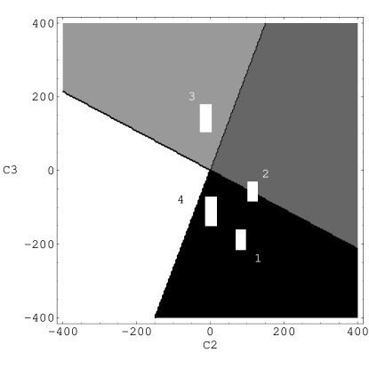
Figure 2: Regions in the $(C_{2}^{(0)},C_{3}^{(0)})$ plane corresponding to each assignment. Each area corresponds to one assignment: #1 (black), #2 (dark grey), #3 (light grey), #4 (white). The line separating the assignments #3,#4 and #2,#1 is given by $3C_{3}^{(0)}+\frac{8}{5}C_{2}^{(0)}=0$, and the line separating the regions for assignments #2,#3 and #1,#4 is $3C_{3}^{(0)}-8C_{2}^{(0)}=0$. The strips show the results for the coefficients $C_{2,3}^{(0)}$ following from the large $N_{c}$ fit in Table 2, for each assignment.

The results of this analysis can be compared directly with a 3-parameter fit performed in CCGL , where only the operators ${\cal O}_{1,2,3}$ were included (see Table V in CCGL ). The only differences are the inclusion of the $\Delta^{*}$ states in CCGL and the fact that the authors of CCGL use in this fit the matrix elements of the operators ${\cal O}_{1,2,3}$ at $N_{c}=3$, while we evaluate them in the large $N_{c}$ limit. The coefficients obtained in CCGL are $N_{c}C_{1}=1626\pm 6$, $C_{2}=75\pm 9$, $C_{3}=-146\pm 17$ (in MeV), and come closest to our assignment #1. However, when all operators up to order $O(1/N_{c})$ are included, the coefficients obtained in CCGL (reproduced here in Table 3) come closest to our assignment #3.

$$\begin{array}[]{ccc|ccccc}\hline\cr N_{c}C_{1}&C_{2}&C_{3}&C_{4}&C_{5}&C_{6}&C_{7}&C_{8}\\ \hline\cr\hline\cr 1389\pm 60&-36\pm 41&123\pm 69&87\pm 97&86\pm 80&438\pm 102&-40\pm 74&48\pm 172\\ \hline\cr\end{array}$$ (51)

Table 3. Results for the coefficients $C_{k}$ (in MeV) obtained from the fit of CCGL , using as input parameters the excited $N$, $\Delta^{*}$ and mixing angles $(\theta_{N1},\theta_{N3})=(0.61,3.04)$ (in rad). Note that our $C_{3}$ is related to that used in CCGL by $C_{3}=C_{3}^{\rm CCGL}/3$.

Beyond leading order in $1/N_{c}$ there are three types of symmetry breaking corrections which introduce deviations from the tower picture:

1. Subleading corrections $C_{1-3}^{(1)}$ in the coefficients of the operators ${\cal O}_{1-3}$.

2. $O(1/N_{c})$ subleading corrections to the matrix elements of the operators ${\cal O}_{2-3}$.

3. Leading contributions from the matrix elements of the ${\cal O}_{4-8}$ operators.

While type 1. corrections just shift the relative position of the towers, the remaining two types of corrections introduce splittings among the tower states. We will include subleading corrections to the matrix elements of the operators ${\cal O}_{1-8}$ by evaluating them at the physical value $N_{c}=3$.

Using as inputs the five masses of the $N^{*}$ states, it would appear at the first sight that there is a 3-dimensional manifold of solutions for the coefficients $C_{1-8}$ of the full set of $O(1/N_{c})$ operators. In fact this is reduced to a 2-dimensional set of solutions because of an accidental relation among the matrix elements of the mass operators with $N_{c}=3$. Namely, when restricted to the subspace of the $N^{*}$ states, a certain linear combination of ${\cal O}_{6,7}$ turns out to be equivalent to the unit operator

$$\langle{\cal O}_{6}\rangle_{N_{c}=3}-\langle{\cal O}_{7}\rangle_{N_{c}=3}=\frac{1}{2}\cdot{\bf 1}\,.$$ (52)

This relation implies an ambiguity in the coefficients $C_{1,6,7}$ beyond leading order in $1/N_{c}$, which can be summarized by noting that the mass spectrum of the $N^{*}$ states is invariant under the simultaneous changes

$$N_{c}C_{1}\to N_{c}C_{1}+\delta\,,\quad C_{6}\to C_{6}-2\delta\,,\quad C_{7}\to C_{7}+2\delta\,.$$ (53)

In other words, only the two combinations $N_{c}C_{1}^{\rm eff}=N_{c}C_{1}-\frac{1}{2}C_{7}$ and $C_{6}^{\rm eff}=C_{6}+C_{7}$ can be determined unambiguously from the $N^{*}$ masses. Of course, the relation (52) is not true anymore when considering also the $\Delta^{*}$ states, which can be used to resolve the ambiguity (53). However, as discussed in Sec. II, due to the incomplete structure of the towers in the $I=3/2$ sector at $N_{c}=3$, the mass spectrum of the observed $\Delta^{*}$ states does not have the correct large $N_{c}$ limiting behaviour. Therefore, we will keep our discussion as general as possible, and present separate results with and without including the $\Delta^{*}$s.

To present the results of our numerical analysis for the coefficients $C_{1-8}$, we need to pick a parameterization of the 2-dimensional manifold of solutions. A particularly convenient choice of the coordinates on this manifold are the mixing angles $(\theta_{N1},\theta_{N3})$, which will be left completely arbitrary. Using as inputs the masses of the five $N^{*}$ states one finds, at each point in the $(\theta_{N1},\theta_{N3})$ plane, one set of coefficients $C_{1,6}^{\rm eff},C_{2-5,8}$. The analytical expressions for these coefficients can be found in the Appendix.

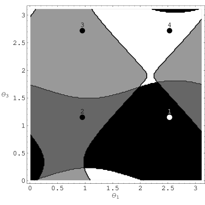
Figure 3: The different regions in the $(\theta_{N1},\theta_{N3})$ plane (in rad) corresponding to the four assignments in Table I, determined as explained in the text. The black region - # 1, dark grey - # 2, light grey - # 3, white - # 4. The four dots shown correspond to the values of the mixing angles in the large $N_{c}$ limit.

It is natural to ask if there is a unique association of a particular solution at a given point $(\theta_{N1},\theta_{N3})$ with one of the four assignments in Table 1. As noted above, the assignment which is realized depends on the large $N_{c}$ values of the cofficients $C_{2,3}^{(0)}$ - see Fig. 2. Requiring that the extracted values of $C_{2,3}(\theta_{N1},\theta_{N3})$ lie inside the regions in Fig. 2 associated with each assignment, one finds the corresponding partition of the entire $(\theta_{N1},\theta_{N3})$ plane into regions shown in Fig. 3. This procedure assumes that the $1/N_{c}$ corrections to the coefficients $C_{2,3}^{(0)}$ are negligible; including them will change slightly the boundaries of the regions in Fig. 3.

Without additional input, the individual coefficients $C_{1-8}$ can not be determined from this $1/N_{c}$ analysis, apart from the rather loose absolute bounds (obtained by varying $\theta_{N1,N3}$ over their entire range $[0,\pi)$): $1374<N_{c}C^{\rm eff}_{1}<1770$, $-148<C_{2}<164$, $-326<C_{3}<363$, $-169<C_{4}<223$, $-169<C_{5}<342$, $-251<C_{6}^{\rm eff}<463$, $-638<C_{8}<775$ (in MeV).

A more precise determination becomes possible if we impose constraints on the parameter space from dimensional analysis. As discussed in Sec. II, the natural size of the coefficients is $C_{k}^{(n)}\sim\Lambda/N_{c}^{n}$. In particular, this means that the coefficients $C_{2,3}$ can not be too different from their large $N_{c}$ values extracted in the previous step (see Table 2). By simple power counting, one expects the $1/N_{c}$ corrections to these coefficients to be of order $\Lambda/N_{c}\sim 150$ MeV. Restricting the coefficients $C_{1-3}$ singles out a solution in the $(\theta_{N1},\theta_{N3})$ plane, resolving the ambiguity (53) and fixing the remaining coefficients $C_{4-8}$.

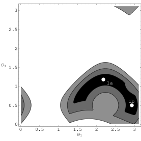
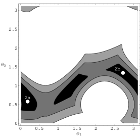
(a)                                             (b)
         
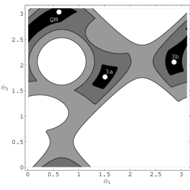
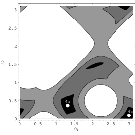
          (c)                                             (d)

Figure 4: Regions in the $(\theta_{N1},\theta_{N3})$ plane corresponding to $(C_{2},C_{3})$ close to the large $N_{c}$ values in Table 2, for each assignment: (a) - # 1, (b) - # 2, (c) - # 3, (d) - # 4. The contour plots are given by max$|C_{2,3}-C_{2,3}^{(0)}|=50,100,150$ MeV.

We present in Fig. 4 the regions allowed from such constraints, for each of the four assignments introduced in Table 1. The regions in the $(\theta_{N1},\theta_{N3})$ plane are obtained from imposing the condition that the coefficients $C_{2,3}(\theta_{1},\theta_{3})$ do not differ by more than 150 MeV from their large $N_{c}$ central values in Table 2. The results for the assignment #4 are given only for illustrative purposes, given that it is ruled out at leading order in $N_{c}$. For example, the black areas in Fig. 4(a) denote the region in the $(\theta_{N1},\theta_{N3})$ plane for which both $C_{2}$ and $C_{3}$ are within 50 MeV from their central values in Table 2, corresponding to the assignment #1. In the $C_{2,3}$ plane (Fig. 2) this region is a square of sides 100 MeV centered on $(83\;{\rm MeV},-188\;{\rm MeV})$. Each lighter shade of grey corresponds to an additional 50 MeV. Similar contour plots are given in Figs. 4(b)-4(d) for each of the remaining three assignments in Table 1. Although the allowed regions appear disjointed, they really form one continuous area because of the doubly periodic conditions in the $(\theta_{N1},\theta_{N3})$ plane.

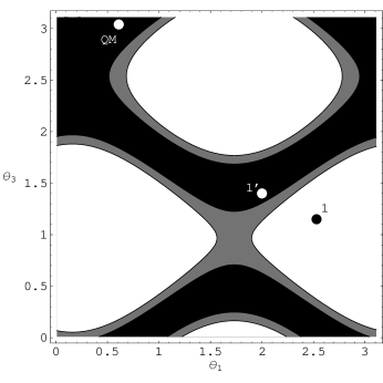
Figure 5: The constraints in the $(\theta_{N1},\theta_{N3})$ plane following from the $\Delta^{*}_{1/2}$ and $\Delta^{*}_{3/2}$ masses. The black (grey) regions correspond to the $\Delta^{*}_{3/2}-\Delta^{*}_{1/2}=75\pm 55$ ($75\pm 80$) MeV.

It is not very illuminating to quote ranges of values for the coefficients $C_{k}$ corresponding to the allowed regions in Figs. 4(a)-(d), since there are significant correlations among coefficients. Instead we give in Table 4 their values at a few representative points in these plots, for each assignment. These points correspond to minimal $1/N_{c}$ corrections to the coefficients $C_{2,3}^{(0)}$ as determined in Table 2 at leading order in $N_{c}$. We quoted the coefficients $C_{1,6,7}$ in a form invariant under the ambiguity (53). One can choose to vary $N_{c}C_{1}$ about its large $N_{c}$ values in Table 2 over a range $\sim\Lambda$, which introduces a large uncertainty in the individual values of $C_{1,6,7}$. On the other hand, the combinations $N_{c}C_{1}^{\rm eff}=N_{c}C_{1}-\frac{1}{2}C_{7}$ and $C_{6}^{\rm eff}=C_{6}+C_{7}$ have smaller errors, of order $\Lambda/N_{c}$.

Finally, to compare with the results of CCGL we consider also the constraints from the $\Delta^{*}$ states. Although these states can not be included in a meaningful way in the large $N_{c}$ fit discussed at the beginning of this section, they can be used to constrain the $1/N_{c}$ determination. Their masses are given explicitly by CCGL

$$\Delta^{*}_{1/2} = N_{c}C_{1}+\frac{1}{3}C_{2}-\frac{4}{9}C_{5}+\frac{2}{3}C_{6}-\frac{1}{3}C_{7}$$ (54)

$$\Delta^{*}_{3/2} = N_{c}C_{1}-\frac{1}{6}C_{2}+\frac{2}{9}C_{5}+\frac{2}{3}C_{6}-\frac{1}{3}C_{7}\,.$$ (55)

Their splitting $\Delta^{*}_{3/2}-\Delta^{*}_{1/2}=-\frac{1}{2}C_{2}+\frac{2}{3}C_{5}=75\pm 80$ MeV gives an allowed region in the $(\theta_{N1},\theta_{N3})$ plane, shown in Fig. 5. This constraint includes the point $(\theta_{N1},\theta_{N3})_{QM}=(0.61,3.04)$ obtained from the quark model fit in CGKM . While most of the region corresponding to the assignment #1 is excluded, this assignment is still marginally allowed (see point $1^{\prime}$ in Fig. 5). Note that each point in the dark area of Fig. 5 gives an acceptable $O(1/N_{c})$ mass matrix of the observed $N^{*}$, $\Delta^{*}$ states, and generalizes the fit of CCGL , which corresponds to the point QM and is obtained by requiring agreement with the quark model mixing angles.

$$\begin{array}[]{c|cc|rrr|rrrr}\hline\cr&\theta_{N1}&\theta_{N3}&N_{c}C_{1}^{\rm eff}&C_{2}&C_{3}&C_{4}&C_{5}&C_{6}^{\rm eff}&C_{8}\\ \hline\cr\hline\cr\#1a&2.18&1.18&1694&83&-187&-5&28&-114&-120\\ \#1b&2.93&0.50&1446&84&-188&-14&-97&333&-272\\ \hline\cr\#2a&0.19&0.58&1466&116&-58&-29&-138&297&-46\\ \#2b&2.72&1.34&1670&115&-58&-125&-56&-71&205\\ \hline\cr\#3a&1.51&1.77&1758&-11&143&41&211&-230&360\\ \#3b&2.86&2.06&1611&-13&142&-111&109&35&451\\ \mbox{QM}&0.61&3.04&1410&-35&123&85&84&398&49\\ \hline\cr\#4a&1.32&0.37&1508&2&-110&186&97&222&-360\\ \#4b&3.00&0.10&1379&2&-110&22&0&454&-245\\ \hline\cr\end{array}$$ (66)

Table 4. Coefficients (in MeV) and angles (in rad) for the points shown in Fig. 4(a)-(d). We also show the quark model point (QM) corresponding to the angles $\theta_{N1,N3}$ used as inputs in CCGL .

IV Conclusions

We studied in this paper the mass spectrum of the $L=1$ orbitally excited nonstrange baryons in the $1/N_{c}$ expansion. In the quark model with spin-flavor independent quark forces, these states fall into the 70 representation of SU(6) su6 . While large $N_{c}$ QCD arguments can be used to reproduce many of the predictions of the quark model for these states in a model-independent way PY1 , they also predict a nontrivial structure of the mass spectrum which breaks spin-flavor symmetry JG . Still, a significant amount of symmetry remains, in the form of the contracted $SU(2N_{f})$ symmetry of large $N_{c}$ QCD DJM1 ; LuMa ; DJM2 . This symmetry predicts that in the large $N_{c}$ limit, the $L=1$ orbitally excited baryons arrange themselves into 3 infinite towers of degenerate states PY1 ; PY2 . These towers are labeled by one integer $T=0,1,2$, and contain all states which satisfy $|J-I|\leq T$.

In a parallel development, the structure of the mass spectrum of the excited baryons was studied in the $1/N_{c}$ expansion JG ; CCGL1 ; CCGL ; SGS ; su3prd using the different but equivalent approach of quark operators. In this approach, the mass operator is written as the most general sum of flavor singlet Lorentz scalar operators which contribute to a given order in $1/N_{c}$. Using such method, the mass spectrum of the $L=1$ baryons was studied in both $SU(2)$ and $SU(3)$ flavor, up to subleading order $O(1/N^{2}_{c})$.

In this paper we show explicitly how the predictions of the $SU(4)_{c}$ symmetry for nonstrange excited baryons follow from the quark mass operator approach in the large $N_{c}$ limit. Apart from recovering the known structure of the mass spectrum in the symmetric limit, this approach allows also the study of the $1/N_{c}$ symmetry breaking corrections. We discuss the special status of the excited $\Delta^{*}$ states in the large $N_{c}$ expansion; for $N_{c}\geq 3$ there are 8 $\Delta^{*}$ states (vs. only 2 at $N_{c}=3$), and their mixing has to be taken into account in order to reproduce the large $N_{c}$ symmetry predictions. This casts some doubt on the ability of the $1/N_{c}$ expansion to correctly describe their properties.

The main aim of our paper is to answer the two (related) questions: a) are the predictions of large $N_{c}$ $SU(2N_{f})_{c}$ symmetry still visible in the observed mass spectrum of the excited baryons? and b) to determine the values of the coefficients of the various operators in the mass operator.

At the first sight, the structure of the observed mass spectrum of the $N^{*}$ states is very similar to the expected set of towers, with states almost degenerate in pairs $\{N_{1/2}(1535),N_{3/2}(1520)\}$, and $\{N_{3/2}(1700),N_{5/2}(1675)\}$. This corresponds to a special assignment of the physical states into $SU(4)_{c}$ representations (#1), and is supported by the full $1/N_{c}$ analysis. This assignment allows for small coefficients for the $O(1/N_{c})$ operators $C_{4-8}$ in the mass matrix (see Table 4, #1a). Even after including the excited $\Delta^{*}$ (see Fig. 5), it is marginally still allowed, in a region around $(\theta_{N1},\theta_{N3})_{\rm 1^{\prime}}\sim(2.0,1.4)$. We conclude that the assignment #1 is still allowed within the present experimental uncertainties.

Allowing for larger $1/N_{c}$ corrections, 3 other assignments of the observed states into large $N_{c}$ towers are possible (see Table 1). We show that model-independent constraints in the large $N_{c}$ limit rule out one of them (#4). The remaining two assignments require (as expected) relatively large coefficients of the $O(N_{c}^{-1})$ operators (see Table 4), depending on the precise position in the $(\theta_{N1},\theta_{N3})$ parameter space. Beyond leading order in $N_{c}$ there is a double continuum of coefficients $C_{k}(\theta_{N1},\theta_{N3})$ (with one additional ambiguity when excluding the $\Delta^{*}$ states). We use dimensional analysis to study the regions in the parameter space where the $1/N_{c}$ expansion is well behaved (see Figs. 4).

We find that, despite requiring large $O(N_{c}^{-1})$ coefficients, the assignment #3 is currently favored by the constraints from the $\Delta^{*}$ mass splittings. This agrees with the results of the fit in CCGL , where a special solution for the coefficients of the mass operator was determined using as inputs the masses and mixing angles of the orbitally excited $N^{*}$, $\Delta^{*}$ states. The specific pattern of the operator coefficients in this fit was invoked in the literature OPE ; Riska as supporting a model of interquark forces based on Goldstone boson exchange (as opposed to one-gluon exchange). Although clearly interesting, we find that it is premature to draw any such conclusions based on the large $N_{c}$ expansion. As noted above, even in the large $N_{c}$ limit, the mass operator can be determined only with discrete ambiguities; at subleading order this becomes a double (triple) continuous ambiguity, depending on whether the $\Delta^{*}$ states are (are not) included.

Further progress towards resolving this multiple ambiguity can be made by considering also the strong couplings of these states. In the large $N_{c}$ limit, these were shown to be related to the assignment of the physical states into large $N_{c}$ towers PY1 . Unfortunately, the precision of the present data is still not sufficient to resolve the ambiguity PY2 . Progress can also come from lattice QCD, from which first results on excited nucleons are already available lattice . As discussed in Sec. III, the specific assignment realized in Nature depends on the values of the large $N_{c}$ coefficients $C_{2,3}^{(0)}$, which could be computed in a lattice simulation. Finally, improvements in the experimental uncertainties in the masses of these states (which will be available from Jefferson Lab in the next future) could sharpen the constraints presented here. Clearly, more than forty years after their discovery, the orbitally excited baryons remain an active and exciting field of study.

Note added: After completing this paper we became aware of similar work on the leading $N_{c}$ mass spectrum of excited baryons done in CoLe .

We are grateful to José Goity for useful discussions, to Elizabeth Jenkins for comments on the manuscript, and to the organizers of the workshop ‘The Phenomenology of Large $N_{c}$ QCD’, Tempe, AZ 2002, where this work was initiated. D.P. acknowledges the hospitality of the Jefferson Laboratory and the Duke University physics department during the final phase of this work. This work has been supported by the DOE and NSF under Grants No. DOE-FG03-97ER40546 (D.P.), NSF PHY-9733343, DOE DE-AC05-84ER40150 and DOE-FG02-96ER40945 (C.S.).

Appendix A Coefficients

We give here the explicit results for the coefficients $C_{1-8}(\theta_{N1},\theta_{N3})$ used in Sec. III. We denote in these expressions $t_{1}=\tan\theta_{N1}$ and $t_{3}=\tan\theta_{N3}$.

$$C_{2}(\theta_{N1},\theta_{N3}) = \frac{1}{3(1+t_{1}^{2})(1+t_{3}^{2})}\left\{(1+t_{3}^{2})(-2t_{1}^{2}+t_{1})N(1650)+(1+t_{1}^{2})(\sqrt{10}t_{3}+2t_{3}^{2})N(1700)\right.$$ (67)

$$\left.-(1+t_{1}^{2})(-2+\sqrt{10}t_{3})N(1520)-(2+t_{1})(1+t_{3}^{2})N(1535)\right\}$$

$$C_{3}(\theta_{N1},\theta_{N3}) = \frac{2}{15(1+t_{1}^{2})(1+t_{3}^{2})}\left\{5(1+4t_{1})(1+t_{3}^{2})N(1650)\right.$$ (68)

$$\left.+(-8-4\sqrt{10}t_{3})(1+t_{1}^{2})N(1700)+(4\sqrt{10}t_{3}-8t_{3}^{2})(1+t_{1}^{2})N(1520)\right.$$

$$\left.+(-20t_{1}+5t_{1}^{2})(1+t_{3}^{2})N(1535)+3(1+t_{1}^{2})(1+t_{3}^{2})N(1675)\right\}$$

$$C_{4}(\theta_{N1},\theta_{N3}) = -\frac{1}{15(1+t_{1}^{2})(1+t_{3}^{2})}\left\{5(1-4t_{1}^{2})(1+t_{3}^{2})N(1650)\right.$$ (69)

$$\left.-9(1+t_{1}^{2})(1+t_{3}^{2})N(1675)+4(1+t_{1}^{2})(1+5t_{3}^{2})N(1700)\right.$$

$$\left.+5(-4+t_{1}^{2})(1+t_{3}^{2})N(1535)+4(1+t_{1}^{2})(5+t_{3}^{2})N(1520)\right\}$$

$$C_{5}(\theta_{N1},\theta_{N3}) = -\frac{1}{20(1+t_{1}^{2})(1+t_{3}^{2})}\left\{5(3+2t_{1}-4t_{1}^{2})(1+t_{3}^{2})N(1650)\right.$$

$$\left.-27(1+t_{1}^{2})(1+t_{3}^{2})N(1675)+(1+t_{1}^{2})(12+10\sqrt{10}t_{3}+20t_{3}^{2})N(1700)\right.$$

$$\left.+2(10-5\sqrt{10}t_{3}+6t_{3}^{2})(1+t_{1}^{2})N(1520)+5(1+t_{3}^{2})(-4-2t_{1}+3t_{1}^{2})N(1535)\right\}$$

$$C_{6}(\theta_{N1},\theta_{N3}) + 6C_{1}(\theta_{N1},\theta_{N3})=\frac{1}{6(1+t_{1}^{2})(1+t_{3}^{2})}\left\{(2+t_{1}^{2})(1+t_{3}^{2})N(1535)\right.$$ (71)

$$\left.+(1+2t_{1}^{2})(1+t_{3}^{2})N(1650)+3(1+t_{1}^{2})(1+t_{3}^{2})N(1675)\right.$$

$$\left.+2(1+2t_{3}^{2})(1+t_{1}^{2})N(1700)+2(2+t_{3}^{2})(1+t_{1}^{2})N(1520)\right\}$$

$$C_{7}(\theta_{N1},\theta_{N3}) - 6C_{1}(\theta_{N1},\theta_{N3})=\frac{1}{3(1+t_{1}^{2})(1+t_{3}^{2})}\left\{(-4+t_{1}^{2})(1+t_{3}^{2})N(1535)\right.$$ (72)

$$\left.+(1-4t_{1}^{2})(1+t_{3}^{2})N(1650)+3(1+t_{1}^{2})(1+t_{3}^{2})N(1675)\right.$$

$$\left.+2(1-4t_{3}^{2})(1+t_{1}^{2})N(1700)+2(-4+t_{3}^{2})(1+t_{1}^{2})N(1520)\right\}$$

$$C_{8}(\theta_{N1},\theta_{N3}) = -\frac{1}{10(1+t_{1}^{2})(1+t_{3}^{2})}\left\{(40+8\sqrt{10}t_{3})(1+t_{1}^{2})N(1700)\right.$$ (73)

$$\left.+(40t_{1}-25t_{1}^{2})(1+t_{3}^{2})N(1535)+(1+t_{1}^{2})(-8\sqrt{10}t_{3}+40t_{3}^{2})N(1520)\right.$$

$$\left.-5(5+8t_{1})(1+t_{3}^{2})N(1650)-15(1+t_{1}^{2})(1+t_{3}^{2})N(1675)\right\}\,.$$

References

- (1) D. Faiman and D. Plane, Nucl. Phys. B 50, 379 (1972); R. R. Horgan and R. H. Dalitz, Nucl. Phys. B 66, 135 (1973); B 71, 514 (1974); B 71, 546 (1974); M. Jones, R. H. Dalitz and R. R. Horgan, Nucl. Phys. B 129, 45 (1977).
- (2) A. J. G. Hey, P. J. Litchfield and R. J. Cashmore, Nucl. Phys. B 95, 516 (1975).
- (3) N. Isgur and G. Karl, Phys. Lett. B72, 109 (1977); Phys. Rev. D18, 4187 (1978).
- (4) C. P. Forsyth and R. E. Cutkosky, Z. Phys. C 18, 219 (1983); S. Capstick and N. Isgur, Phys. Rev. D 34, 2809 (1986).
- (5) L. Ya. Glozman and D. O. Riska, Phys. Rept. 268, 263 (1996).
- (6) H. Collins and H. Georgi, Phys. Rev. D 59, 094010 (1999).
- (7) D. O. Riska, arXiv:nucl-th/9908065.
- (8) R. F. Dashen and A. V. Manohar, Phys. Lett. B 315, 425 (1993); R. F. Dashen and A. V. Manohar, Phys. Lett. B 315, 438 (1993); E. Jenkins, Phys. Lett. B 315, 441 (1993).
- (9) M. A. Luty and J. March-Russell, Nucl. Phys. B 426, 71 (1994).
- (10) R. Dashen, E. Jenkins and A. V. Manohar, Phys. Rev. D49, 4713 (1994); D51, 3697 (1995).
- (11) G. t’Hooft, Nucl. Phys. B72, 461 (1974).
- (12) E. Witten, Nucl. Phys. B160, 57 (1979).
- (13) C. D. Carone, H. Georgi, L. Kaplan and D. Morin, Phys. Rev. D50, 5793 (1994).
- (14) J. L. Goity, Phys. Lett. B 414, 140 (1997).
- (15) D. Pirjol and T. M. Yan, Phys. Rev. D57, 1449 (1998).
- (16) D. Pirjol and T. M. Yan, Phys. Rev. D57, 5434 (1998).
- (17) C. E. Carlson, C. D. Carone, J. L. Goity and R. F. Lebed, Phys. Lett. B438, 327 (1998).
- (18) C. E. Carlson, C. D. Carone, J. L. Goity and R. F. Lebed, Phys. Rev. D59, 114008 (1999).
- (19) C. E. Carlson and C. D. Carone, Phys. Rev. D 58, 053005 (1998); C. E. Carlson and C. D. Carone, Phys. Lett. B 441, 363 (1998).
- (20) C. L. Schat, J. L. Goity and N. N. Scoccola, Phys. Rev. Lett. 88, 102002 (2002).
- (21) J. L. Goity, C. L. Schat and N. N. Scoccola, Phys. Rev. D 66, 114014 (2002).
- (22) S. Sasaki, T. Blum and S. Ohta, Phys. Rev. D 65, 074503 (2002); W. Melnitchouk et al., arXiv:hep-lat/0202022; Nucl. Phys. Proc. Suppl. 109, 96 (2002); D. G. Richards et al., (QCDSF/UKQCD/LHPC Coll.), Nucl. Phys. Proc. Suppl. 109, 89 (2002).
- (23) T. D. Cohen and R. F. Lebed, arXiv:hep-ph/0301167.