Effective theories and constraints on new physics

Abstract

Anomalous moments of the top quark arises from one loop corrections to the vertices $\bar{t}tg$ and $\bar{t}t\gamma$. We study these anomalous couplings in different frameworks: effective theories, Standard Model and 2HDM. We use available experimental results in order to get bounds on these anomalous couplings.

1 Introduction

The top quark is the heaviest fermion in the standard model (SM) with a mass of $174.3\pm 5.1$ GeV top. In the framework of the SM, the couplings of the top quark are fixed by the gauge symmetry. Anomalous couplings between the top quark and gauge bosons might affect the top quark production at high energies and also its decay rate. Precisely measured quantities with virtual top quark contributions will yield further information regarding these couplings.

Since the top quark mass is so heavy, it is expected that its physics may be different from the lighter fermions and that the top quark might couple quite strongly to the electroweak symmetry breaking sector. This suggests the SM is just an effective theory and that the physics beyond the SM may be manifested through an effective Lagrangian involving the top quark.

The framework of effective theories, as a mean to parametrize physics beyond the SM in a model independent way, has been used recently. Two cases have been consider in the literature, the decoupling case, which includes the Higgs boson, and the non-decoupling case, where there is not any Higgs boson. We shall consider only the first case, in which the SM is a low-energy limit of a renormalizable theory. In this approach, the effective theory parametrizes the effects at low energy of the full renormalizable theory by means of high order dimensional non-renormalizable operators georgi.

The effective Lagrangian approach is a convenient model independent parametrization of the low-energy effects of the new physics that may show up at high energies. Effective Lagrangians, employed to study processes at a typical energy scale $E$ can be written as a power series in $1/\Lambda$, where the scale $\Lambda$ is associated with the heavy particles masses of the underlying theory london. The coefficients of the different terms in the effective Lagrangian arise from integrating out the heavy degrees of freedom. In order to define an effective Lagrangian it is necessary to specify the symmetry and the particle content of the low-energy theory. In our case, we require the effective Lagrangian to be $CP$-conserving, invariant under SM symmetry $SU(2)_{L}\otimes U(1)_{Y}$, and to have as fundamental fields the same ones appearing in the SM spectrum. Therefore we consider a Lagrangian in the form

$${\cal L}_{eff}={\cal L}_{SM}+\sum_{n}\alpha_{n}{\cal O}^{n}$$ (1)

where the operators ${\cal O}^{n}$ are of dimension greater than four.

2 The anomalous magnetic moment

The aim now is to extract indirect information on the magnetic dipole moment of the top quark from LEP data, specifically we use the ratios $R_{b}$ and $R_{l}$ defined by

$$R_{b}=\frac{\Gamma(Z\rightarrow b\bar{b})}{\Gamma(Z\rightarrow hadron)}\;,\qquad R_{l}=\frac{\Gamma(Z\rightarrow hadron)}{\Gamma(Z\rightarrow l\bar{l})},\;\Gamma_{Z}$$ (2)

in the context of an effective Lagrangian approach. The oblique and QCD corrections to the $b$ quark and hadronic $Z$ decay widths cancel off in the ratio $R_{b}$. This property makes $R_{b}$ very sensitive to direct corrections to the $Zb\overline{b}$ vertex, specially those involving the heavy top quark , while $\Gamma_{Z}$ and $R_{l}$ are more sensitive to the oblique corrections.

In the present work, we consider the following dimension six and $CP$-conserving operators,

$$O_{uW}^{ab}=\bar{Q}_{L}^{a}\sigma^{\mu\nu}W_{\mu\nu}^{i}\tau^{i}\tilde{\phi}U_{R}^{b}\;,\qquad O_{uB}^{ab}=\bar{Q}_{L}^{a}\sigma^{\mu\nu}YB_{\mu\nu}\tilde{\phi}U_{R}^{b}\;,$$ (3)

where $Q_{L}^{a}$ is the quark isodoublet, $U_{R}^{b}$ is the up quark isosinglet, $a$ , $b$ are the family indices, $B_{\mu\nu}$ and $W_{\mu\nu}$ are the $U(1)_{Y}$ and $SU(2)_{L}$ field strengths, respectively, and $\tilde{\phi}=i\tau_{2}\phi^{\ast}$. We use the notation introduced by Buchmüller and Wyler wyler. After spontaneous symmetry breaking, these fermionic operators generate also effective vertices proportional to the anomalous magnetic moments of quarks. The above operators for the third family give rise to the anomalous $t\bar{t}\gamma$ vertex and the unknown coefficients $\epsilon_{uB}^{ab}$ and $\epsilon_{uW}^{ab}$ are related with the anomalous magnetic moment of the top quark through

$$\delta\kappa_{t}=-\sqrt{2}{\frac{m_{t}}{m_{W}}}\frac{g}{eQ_{t}}(s_{W}\epsilon_{uW}^{33}+c_{W}\epsilon_{uB}^{33})\;,$$ (4)

where $s_{W}$ denotes the sine of the weak mixing angle.

The expression for $R_{b}$ is given by

$$R_{b}=R_{b}^{SM}(1+(1-R_{b}^{SM})\delta_{b})\;,$$ (5)

where $R_{b}^{SM}$ is the value predicted by the SM and $\delta_{b}$ is the factor which contains the new physics contribution, and it is defined as follows

$$\delta_{b}={\frac{2\left({g_{V}^{SM}g_{V}^{NP}+g_{A}^{SM}g_{A}^{NP}}\right){+}\left({g_{V}^{NP}}\right)^{2}{+}\left({g_{A}^{NP}}\right)^{2}}{{(g_{V}^{SM})^{2}+(g_{A}^{SM})^{2}}}}$$ (6)

and $g_{V}^{SM}$ and $g_{A}^{SM}$ are the vector and axial vector couplings of the $Zb\bar{b}$ vertex. The contributions from new physics, eq. (3), to $R_{l}$ and $\Gamma_{Z}$ are of two classes. One from vertex correction to $Zb\bar{b}$ in the $\Gamma_{hadr}$ and the other from the oblique correction through $\Delta\kappa$ in the $\sin^{2}\theta_{W}$. These can be written as

$$R_{l} = R_{l}^{SM}(1-0.1851\;\Delta\kappa+0.2157\;\delta_{b})\;,$$

$$R_{b} = R_{b}^{SM}(1-0.03\;\Delta\kappa+0.7843\;\delta_{b})\;,$$

$$\Gamma_{Z} = \Gamma_{Z}^{SM}(1-0.2351\;\Delta\kappa+0.1506\;\delta_{b})$$ (7)

where $\Delta\rho$ is equal to zero for the operators that we are considering.

We will consider the one loop contribution of the above effective operators to the $Zb\overline{b}$ vertex. After evaluating the Feynman diagrams, with insertions of the effective operators $O_{uB}^{ab}$ and $O_{uW}^{ab}$ we obtain

$$g_{V}^{NP} = 4\sqrt{2}\epsilon_{uW}^{33}G_{F}m_{W}^{3}m_{t}\big{\{}3c_{W}(\tilde{C}_{12}-\tilde{C}_{11})-{\frac{m_{t}^{2}}{\sqrt{2}m_{W}^{2}}}(C_{12}-C_{11}+C_{0})$$

$$+{\frac{(1+a)}{8c_{W}}}(C_{11}+C_{12}+C_{0})+\frac{1}{\sqrt{2}}(C_{12}-C_{11}-C_{0})$$

$$-\frac{3a}{4c_{W}m_{Z}^{2}}(B_{1}-B_{0})\big{\}},$$

$$g_{A}^{NP} = 4\sqrt{2}\epsilon_{uW}^{33}G_{f}m_{W}^{3}m_{t}\big{\{}-{\frac{a}{2c_{W}}}(C_{0}+C_{12}-C_{11})$$ (8)

$$- \frac{1}{\sqrt{2}}(C_{12}-C_{0}-C_{11})+\frac{m_{t}^{2}}{\sqrt{2}m_{W}^{2}}(C_{12}-C_{11}+C_{0})$$

$$-{\frac{2m_{t}s_{W}^{2}}{m_{W}}}(\tilde{C}_{0}+\tilde{C}_{12}-\tilde{C}_{11})-\frac{3}{4c_{W}m_{Z}2}(B_{1}-B_{0})\big{\}}\;$$

for the operator $O_{uW}$ and,

$$g_{V}^{NP} = g_{A}^{NP}=\frac{4\sqrt{2}}{3}\epsilon_{uB}^{33}G_{F}m_{W}^{3}m_{t}\frac{s_{W}}{c_{W}}[\frac{m_{t}^{2}}{\sqrt{2}m_{W}^{2}}(C_{12}-C_{11}+C_{0})$$ (9)

$$-\frac{1}{\sqrt{2}}(-C_{11}+C_{12}-C_{0})]\;,$$

for the $O_{uB}$. In the above equations $a=1-{\frac{8}{3}}s_{W}^{2}$ while $C_{ij}=C_{ij}(m_{W},m_{t},m_{t})$, $\tilde{C}_{ij}=\tilde{C}_{ij}(m_{t},m_{W},m_{W})$ and $B_{i}=B_{i}(0,m_{t},m_{W})$ are the Passarino-Veltman scalar integral functions veltman. The combination $B_{0}-B_{1}$ has a pole in $d=4$ dimensions that is identified with the logarithmic dependence and can be replaced by $\ln\Lambda^{2}/m_{Z}^{2}$.

Now we have various posibilities to explore the space of the parameters $\varepsilon_{uW}^{33}$, $\varepsilon_{uB}^{33}$ and $\delta\kappa_{t}$. Using experimental values for $\Gamma_{Z}$, $R_{b}$ and $R_{l}$ we find the allowed region in the plane $\varepsilon_{uW}^{33}-$ $\varepsilon_{uB}^{33}.$ If we do not neglect the term of the order $\left(g^{NP}\right)^{2}$, we get the following expressions

$$-0.057\varepsilon_{B}+0.058\varepsilon_{B}^{2}+0.053\varepsilon_{W}+0.0015\varepsilon_{W}^{2}+0.01\varepsilon_{B}\varepsilon_{W} = 1-(\Gamma_{Z}^{\exp}/\Gamma_{Z}^{SM}),$$

$$-0.023\varepsilon_{B}+0.026\varepsilon_{B}^{2}+0.016\varepsilon_{W}+0.0007\varepsilon_{W}^{2}+0.0048\varepsilon_{B}\varepsilon_{W} = 1-(R_{b}^{\exp}/R_{b}^{SM}),$$

$$-0.656\varepsilon_{B}+0.686\varepsilon_{B}^{2}+0.536\varepsilon_{W}+0.018\varepsilon_{W}^{2}+0.1264\varepsilon_{B}\varepsilon_{W} = 1-(R_{l}^{\exp}/R_{l}^{SM}),$$

where we have omitted the superindex $33$.

The SM values for the parameters that we have used are

$$\Gamma_{Z} = 2.4963GeV,\;\;R_{l}=20.743,$$

$$R_{b} = 0.21572,\Gamma_{hadr}=17427MeV,\;\;\Gamma_{l}=84.018MeV,$$

with the input parameters:

$$m_{t} = 174.3GeV,\;\;\alpha_{s}(m_{Z})=0.118,$$

$$m_{Z} = 91.1861GeV,\;\;m_{H}=100GeV,\;\;\Lambda=1TeV.$$

And the experimental values are

$$\Gamma_{Z} = 2.4952\pm 0.0023GeV,\;\;R_{l}=20.804\pm 0.050,$$

$$R_{b} = 0.21653\pm 0.00069.$$

After doing a $\chi^{2}$ analysis at $95\%$ C.L. we find the allow region for $\varepsilon_{uW}^{33}-$ $\varepsilon_{uB}^{33}$ parameters. In this kind of scenarios new physics is explored assuming that its effects are smaller than the SM effects, consequently one expect that $\left|g_{V,A}^{NP}/g_{V,A}^{SM}\right|\ll 1$ and, then we get the inequalities $\left|\varepsilon_{uW}^{33}\right|\leq 0.11,$ $\left|\varepsilon_{uB}^{33}\right|\leq 0.48$. By using the eq. $(4)$ and the bounds got in the numerical analysis, we obtain for $\delta\kappa_{t}$ the following values

$$-2.94\leq \delta\kappa_{t} \leq 1.3,\;-0.76\leq\delta\kappa_{t}\leq 1.9,$$

$$-1.3\leq \delta\kappa_{t} \leq 1.7$$ (10)

which correspond to $\Gamma_{Z},\$ $R_{b}$ and $R_{l}$, respectively. Therefore for these observables $\Gamma_{Z},\$ $R_{b}$ and $R_{l}$, we get the allowed region

$$-2.94\leq\delta\kappa_{t}\leq 1.9.$$ (11)

3 Anomalous chromomagnetic dipole moment I

We are interested in studying possible deviations from the SM on the decay $b\to s\gamma$ within the context of the effective Lagrangian approach. Several authors have been used the CLEO results on radiative $B$ decays to set bounds on the anomalous coupling of the t-quark. We will use dimension-six operator which are full strong and electroweak gauge invariant and contribute to $b\to s\gamma$ in order to bound the chromomagnetic dipole moment of the top quark.

Since the anomalous chromomagnetic dipole moment of the top quark appears in the top quark cross section, it is possible, due to uncertainties, to estimate the constraints that it would impose on the $\Delta\kappa_{g}^{t}$. For the LHC, the anomalous coupling is constrained to lie in the range $-0.09\leq\Delta\kappa_{g}^{t}\leq 0.1$ atwood. Similar range is obtained for the future NLC. The influence of an anomalous $\Delta\kappa$ on the cross section and associated gluon jet energy for $t\bar{t}g$ has been also analyzed. Events produced at $500$ GeV in $e^{+}e^{-}$ colliders, with a cut on the gluon energy of $500$ GeV and integrated luminosity of $30fb^{-1}$, lead to a bound of $-2.1\leq\Delta\kappa_{g}^{t}\leq 0.6$ atwood.

¿From the experimental information it is possible to get a limit on the $\Delta\kappa_{g}^{t}$ from Tevatron. Following the reference by F. del Aguila aguila and assuming that the only non-zero coupling is precisely the chromomagnetic dipole moment of the top quark, we find from the collected data that the allowed region is $|\Delta\kappa_{g}^{t}|\leq 0.45$.

We consider the following dimension-six, CP-conserving operators, which are $SU(3)_{C}\otimes S(2)_{L}\otimes U(1)_{Y}$ gauge invariant

$${\cal O}^{ab}_{uG}=\bar{Q}_{L}^{a}\sigma_{\mu\nu}G^{\mu\nu\;i}\frac{\lambda^{i}}{2}\tilde{\phi}u_{R}^{b}\;,$$ (12)

where $G^{\mu\nu\;i}$ is the gluon field strength tensor and $a,b$ are the family indices. The above operator gives rise to the anomalous $t\bar{t}g$ vertex and its respective unknown coefficient $\epsilon_{ab}^{uG}$ is related with the anomalous chromomagnetic moment of the top quark by

$$\delta\kappa^{t}_{g}=\sqrt{2}\frac{g}{g_{s}}\frac{m_{t}}{M_{W}}\epsilon_{uG}^{33}\;.$$ (13)

where by means of the dimension 5 coupling to an on-shell gluon, the anomalous chromomagnetic dipole moment of the top quark is defined as

$$L_{5}=i(\frac{\Delta\kappa_{g}^{t}}{2})\frac{g_{s}}{2m_{t}}\bar{u}(t)\sigma_{\mu\nu}q^{\nu}T^{a}u(t)G^{\mu,a}$$ (14)

with $g_{s}$ and $T^{a}$ are the $SU(3)_{c}$ coupling and generators, respectively.

The effective Hamiltonian used to compute the $b\to s$ transition is given by buras

$$H_{eff}=-\frac{4G_{F}}{\sqrt{2}}V_{ts}^{*}V_{tb}\sum_{i=1}^{8}c_{i}(\mu){\cal O}_{i}(\mu)\;,$$ (15)

where $\mu$ is the energy scale at which $H_{eff}$ is applied. For $i=1-6$, ${\cal O}_{i}(\mu)$ correspond to four-quark operators, ${\cal O}_{7}(\mu)$ is the electromagnetic dipole moment and ${\cal O}_{8}(\mu)$ is the chromomagnetic dipole operator. At low energy, $\mu\approx m_{b}$, the only operator that contributes to $b\to s$ transition is ${\cal O}_{7}(\mu)$ which results from a mixing among the ${\cal O}_{2}(M_{W})$, ${\cal O}_{7}(M_{W})$ and ${\cal O}_{8}(M_{W})$ operators.

The total contribution of the effective operator (12) to the ${\cal O}_{8}(M_{W})$ operator can be written as:

$$c_{8}(M_{W})=c_{8}(M_{W})^{SM}+\delta\kappa_{g}^{t}\Delta c_{8}(M_{W})\;,$$ (16)

where

$$\Delta c_{8}(M_{W}) = \frac{1}{4V_{ts}}\ln\left(\frac{\Lambda^{2}}{M_{W}^{2}}\right)+\frac{1}{V_{ts}}\frac{x-x^{2}+x(2-x)\ln(x)}{8(1-x)^{2}}$$ (17)

$$+ \frac{3x-4x^{2}+x^{3}+2x\ln(x)}{8(1-x)^{3}}$$

and $x=m_{t}^{2}/M_{W}^{2}$.

Using the recent data from CLEO collaboration for the branching fraction of the process $B(b\to s\gamma)=(3.21\pm 0.43\pm 0.27)\times 10^{-4}$ cleo, we get an allowed region for the anomalous chromomagnetic dipole moment of the top quark to be nos

$$-0.03\leq\Delta\kappa_{g}^{t}\leq 0.01$$ (18)

4 Anomalous chromomagnetic dipole moment II

Our next objective is to evaluate the contribution at the one loop-level to the anomalous chromomagnetic dipole moment of the top quark in different scenarios with the gluon boson on-shell. Beginning with the SM, the typical QCD correction through gluon exchange implies two different Feynman diagrams. After the explicit calculation of the loops, we find that

$$\Delta\kappa_{g}^{t}=-\frac{1}{6}\frac{\alpha_{s}(m_{t})}{\pi}.$$ (19)

We note that its natural size is of the order of $\alpha_{s}/\pi$ similar to the QED anomalous coupling, but now in combination with a factor $-1/6$ coming from the color structure in the diagram i.e. $T^{a}T^{b}T^{a}=-T^{b}/6$ with $T^{a}$ being the generators of $SU(3)_{C}$.

The other possible contribution in the framework of the SM comes from electroweak interactions. The relevant contributions occur when neutral Higgs boson and the would-be Goldstone boson of $Z$ are involved in the loop. This contribution reads

$$\Delta\kappa_{g}^{t}=-\frac{\sqrt{2}G_{F}m_{t}^{2}}{8\pi^{2}}[H_{1}(m_{h})+H_{2}(m_{Z})],$$ (20)

where

$$H_{1}(m) = \int_{0}^{1}dx\frac{x-x^{3}}{x^{2}-(2-m^{2}/m_{t}^{2})x+1},$$

$$H_{2}(m) = \int_{0}^{1}dx\frac{-x+2x^{2}-x^{3}}{x^{2}-(2-m^{2}/m_{t}^{2})x+1}.$$

The SM contribution is showed in figure 1 where we have added the QCD contribution. It is worth noting that the behaviour of the curve for a large Higgs boson mass indicates decoupling and that the values of $\Delta\kappa_{g}^{t}$ lie within the allowed region for $\Delta\kappa_{g}^{t}$ coming from $b\to s\gamma$.

The contributions within a general 2HDM will be different from the SM contributions because of the presence of the virtual five physical Higgs bosons which appear in any two Higgs doublet model after spontaneous symmetry breaking: $H^{0}$, $A^{0}$, $h^{0}$, $H^{\pm}$ doshiggs. Therefore, 2HDM predictions depend on their massses and on the two mixing angles $\alpha$ and $\beta$. For small $\beta$, the charged Higgs boson contribution is suppressed due to its large mass and the small bottom quark mass.

The expression for the contribution of the neutral Higgs bosons is given by

$$\Delta\kappa_{g}^{t} = \frac{\sqrt{2}G_{F}}{8\pi^{2}}[\lambda_{H^{0}tt}^{2}H_{1}(M_{H}^{2})+\lambda_{h^{0}tt}^{2}H_{1}(M_{h}^{2})$$ (21)

$$+ \lambda_{A^{0}tt}^{2}H_{2}(M_{A}^{2})+\lambda_{G^{0}tt}^{2}H_{2}(M_{Z}^{2})]$$

where $\lambda_{itt}$ are the Yukawa couplings in the so-called models of type I, II and III . Table I shows the couplings in the usual convention.

$\lambda_{itt}$	model type I	model type II	model type III
$\lambda_{H^{0}tt}$	$\frac{m_{t}\sin\alpha}{\sin\beta}$	$\frac{m_{t}\cos\alpha}{\cos\beta}$	$(1+\frac{\eta^{U}_{tt}}{\sqrt{2}})m_{t}\sin\alpha$
$\lambda_{h^{0}tt}$	$\frac{m_{t}\cos\alpha}{\sin\beta}$	$\frac{m_{t}\sin\alpha}{\cos\beta}$	$(1+\frac{\eta^{U}_{tt}}{\sqrt{2}})m_{t}\cos\alpha$
$\lambda_{A^{0}tt}$	$\cot\beta m_{t}$	$\tan\beta m_{t}$	$\frac{\eta^{U}_{tt}m_{t}}{\sqrt{2}}$
$\lambda_{G^{0}tt}$	$m_{t}$	$m_{t}$	$m_{t}$

Table 1: Couplings of the Higgs eigenstates with the top quark in 2HDM. We omit the factor $g/2m_{W}$ and in the model type III we use the Sher-Cheng approach for the flavour changing couplings.

The Yukawa couplings of a given fermion to the Higgs scalars are proportional to the mass of the fermion and they are therefore naturally enhanced in this case. In the model type III appears flavour changing neutral couplings at tree level which can be parametrized in the Sher-Cheng approach where a natural value for the flavour changing couplings from different families should be of the order of the geometric average of their Yukawa couplings, $h_{ij}=g\eta_{ij}\sqrt{m_{i}m_{j}}/(2m_{W})$ with $\eta_{ij}$ of the order of one.

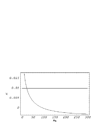
Figure 1: Standar Model contribution to the anomalous cromomagnetic dipole moment of the top quark vs the higgs boson mass

In order to show the behaviour of the contribution of the 2HDM to the anomalous chromomagnetic dipole moment of the top quark, we evaluate explicitly the contribution for couplings type II. We show in figure 2 the allowed region (above the curve) for the plane $\tan\beta$ vs $m_{H}$ using equation (21) and assuming that $-0.03\leq\Delta\kappa_{g}^{t}\leq 0.01$ from $b\to s\gamma$. We fix the following parameters: $m_{H}=m_{h}$, $m_{A}=200(400)$ GeV solid line (dashed line). The solid line for the scalar Higgs mass smaller (bigger) than $240$ GeV corresponds to the cut between equation (21) and the upper(lower) limit from $b\to s\gamma$.

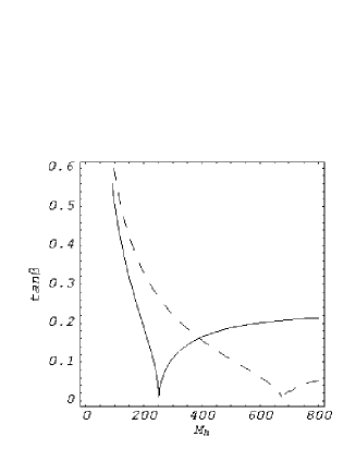
Figure 2: Contour plot for the contribution of 2HDM to the anomalous cromomagnetic dipole moment of the top quark in the plane $\tan\beta-m_{H}$ for $M_{A}=200$ GeV(solid line) and $M_{A}=400$ GeV (dashed line) using the bound from the $b\to s\gamma$ process. The allowed region is above the curve