The QCD factorization in $B\to DKK$ decays

Abstract

A study of hadron pair production mechanism is motivated by the recent observed decays $\bar{B}^{0}\to D^{(*)+}K^{-}K^{0}$. One novel phenomenon is threshold enhancement of the kaon pair production. We show that these decays in the heavy quark mass limit can be factorized into a generalized form. The new non-perturbative quantity is the generalized distribution amplitude which describes how a quark-antiquark pair transmits into the hadron pair. A proof of factorization of $\bar{B}^{0}\to D^{(*)+}K^{-}K^{0}$ decays to all-orders is performed by using the soft-collinear effective theory. The phenomenological application is discussed in brief.

I Introduction

Recently, the three body charmful decays $B\to D^{(*)}K^{-}K^{(*)0}$ were first observed by the BELLE Collaboration Belle . They also found a novel phenomenon that the mass spectra of the $K^{-}K^{(*)0}$ pair peaks near their mass threshold. In CHST , a factorization approach which extends the conventional (or say, naive) factorization approach in B-meson two body decays BSW was proposed to study $\bar{B}^{0}\to D^{(*)+}K^{-}K^{0}$ decays. The transition matrix element of $\bar{B}^{0}\to D^{(*)+}K^{-}K^{0}$ is factorized into a $B\to D$ form factor multiplied by a $K^{-}K^{0}$ weak form factor. The $K^{-}K^{0}$ form factor is constrained from the experimental data for the time-like electromagnetic (EM) kaon form factors. The branching ratios obtained in this approach agree with the experiment. The phenomenological success indicates that the generalized factorization assumption may be valid as the leading approximation of an asymptotic expansion. The purpose of this study is to establish a theoretical foundation of the factorization for B-meson multi-body decays, in particular for $B\to DKK$ decays in QCD.

The factorization approach for the non-leptonic, two body B-meson decays had been used for a long time BSW . The basic idea is that a hadronic matrix element of the four-quark operator is factorized into a multiplication of two simpler matrix elements which one is represented by a form factor and another by a decay constant. An argument based on “color transparency” was proposed as a mechanism of the factorization Bjorken . The QCD factorization method develops the naive factorization into a rigorous and systematic framework BBNS . The main ingredient is factorization, the separation of perturbative from non-perturbative dynamics, a standard method in perturbative QCD for the hard exclusive processes BL . The naive factorization approach is its lowest order (the strong coupling constant $\alpha_{s}$) approximation. A proof of factorization at two-loop order in $B\to D\pi$ decays is given by using the methods of momentum regions and Ward identities. The all-orders proof is done in the recently developed soft-collinear effective theory B2 . The proof of factorization in the soft-collinear effective theory has several advantages: the explicit gauge invariance at the classical level can be utilized; the operator language is simpler than the diagrammatic analysis; the separation of the perturbative from the non-perturbative dynamics is easily done in effective theory because they occur at disparate energy scales. We will use the soft-collinear effective theory to give a proof of factorization for $\bar{B}^{0}\to D^{(*)+}K^{-}K^{0}$ decays.

The exclusive, non-leptonic three body B meson decays are usually more complicate than two body case. However, the hadronic physics of $\bar{B}^{0}\to D^{(*)+}K^{-}K^{0}$ decays in the heavy quark limit (the heavy quark mass $m_{b}\to\infty$) may be simpler because the final kaon pair has small invariant mass. It is well-known in QCD that the large energy behavior of hadron form factor satisfies a dimensional counting rule BL . Consequently, the probability of kaon pair production at large invariant mass is suppressed by powers of large energy. This phenomenon is called the from factor suppression. Thus the dominant contribution comes from the region with small invariant mass. For the production of kaon pair at small invariant mass, it is analogous to the production mechanism of two pions in the process $\gamma^{*}\gamma\to\pi\pi$ with high virtual photons and small invariant mass of pion pair DGPT . According to this mechanism, $K^{-}K^{0}$ mesons are produced by the hadronization of $\bar{u}d$ pair emitted from the W-boson and can be described by a universal, non-perturbative matrix element which generalizes the standard description of a hadron in QCD BL . The new element is generalized distribution amplitude(s) which is the crossed version of of the generalized parton distribution (GPD) of hadron Ji .

In the small invariant mass region, the two kaons are nearly collinear and energetic. Thus, the argument of “color transparency” is applicable. Since the $\bar{u}d$ pair moves fast, time dilation effect makes the hadronization of kaon pair cannot occur until the $\bar{u}d$ pair moves far away from the remaining system. The transition $\bar{u}d\to K^{-}K^{0}$ with a small invariant mass is soft and is described by a generalized distribution amplitude of kaon pair. For the $B\to D$ transition, the light spectator does not require a hard interaction because B and D mesons are both heavy. The energetic and collinear $\bar{u}d$ pair in a color-singlet configuration decouples from the soft gluon interactions. So, the strong interactions between $K^{-}K^{0}$ and $BD$ systems occur at short distance and can be systematically calculated in perturbative QCD. The above arguments will lead to a factorization form depicted in Fig. 1. Up to leading order of $\frac{w}{m_{b}}$ ($w$ being the kaon pair invariant mass), the hadronic matrix element of a four-quark operator $Q_{i}$ in the weak effective Hamiltonian is expressed as

$$\langle DKK|Q_{i}|\bar{B}\rangle=F^{BD}(w^{2})\int_{0}^{1}dz~{}H_{i}(z)\Phi^{KK}(\zeta,z,w^{2}).$$ (1)

Here, $F^{BD}(w^{2})$ is a $B\to D$ transition form factor at the momentum transfer $w^{2}$, and $\Phi^{KK}(z,\zeta,w^{2})$ is a generalized distribution amplitude (GDA) of the kaon pair. $H$ denotes a hard scattering kernel which is perturbatively calculable. This factorization formulae is a natural generalization of the QCD factorization in $B\to D\pi$ decays given in BBNS . Just as the $B\to D\pi$ decay, the $B\to DKK$ process provides a clean environment to test the factorization in the three body B meson decays.

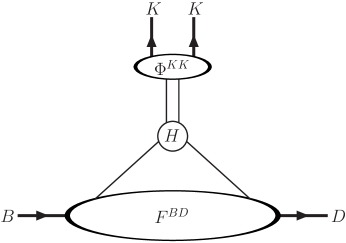
Figure 1: Factorization of process $B\to DKK$ in the large $m_{B}$ limit.

II The factorization in $B\to DKK$ decays

For the sake of illustration, our discussion will concentrate on the decay $\bar{B}^{0}\to D^{+}K^{-}K^{0}$. The extension to $\bar{B}^{0}\to D^{*+}K^{-}K^{0}$ decay can easily performed. We shall work in the rest frame of the B meson. It is convenient to use the light-cone variables $p^{\mu}=(p^{+},p^{-},p_{\bot})=n_{-}\cdot p\frac{n_{+}^{\mu}}{2}+n_{+}\cdot p\frac{n_{-}^{\mu}}{2}+p_{\bot}^{\mu}$ with $n_{+}^{\mu}=(2,0,0_{\bot})$ and $n_{-}^{\mu}=(0,2,0_{\bot})$ are two light-like vectors which satisfy $n_{+}^{2}=n_{-}^{2}=0$, and $n_{+}\cdot n_{-}=2$. Introduce the total momentum of the kaon pair $P=p_{1}+p_{2}$ where $p_{1,2}$ are momenta of the $K^{-},K^{0}$ respectively, and invariant mass $P^{2}=w^{2}$. The momentum $P$ is chosen to be mainly in the “$-$” direction. Define the momentum fraction variable $\zeta\equiv\frac{p_{1}^{-}}{P^{-}}$. Under the above conventions, we have

$$P_{B}=(m_{B},~{}m_{B},~{}\vec{0}_{\bot}),~{}~{}~{}~{}~{}P_{D}=(m_{B},~{}rm_{B},~{}\vec{0}_{\bot}),~{}~{}~{}~{}~{}P=\bar{r}(\eta m_{B},~{}m_{B},~{}\vec{0}_{\bot}),$$

$$p_{1}=\bar{r}(\bar{\zeta}\eta m_{B},~{}\zeta m_{B},~{}\vec{p}_{\bot}),~{}~{}~{}~{}~{}p_{2}=\bar{r}(\zeta\eta m_{B},~{}\bar{\zeta}m_{B},~{}-\vec{p}_{\bot}).$$ (2)

where $r=\frac{m_{D}^{2}}{m_{B}^{2}}$, $\eta=\frac{w^{2}}{(\bar{r}m_{B})^{2}}$ and $p_{\bot}^{2}=(\zeta\bar{\zeta}w^{2}-m_{K}^{2})/\bar{r}^{2}$. We have used the “bar”-notation for any longitudinal momentum fraction variable $\bar{u}=1-u$ throughout this paper. One can obtain the kinematical constraint on the variable $\zeta$: $\zeta\bar{\zeta}\geq\frac{m_{K}^{2}}{\bar{r}^{2}w^{2}}$.

We consider the kinematic region

$$w^{2}\ll m_{B}^{2}.$$ (3)

This requirement is guaranteed by the form factor suppression at large invariant mass. We will give an argument of the suppression later.

The factorization of $B\to D\pi$ decays in the soft-collinear effective theory was studied in B2 ; B3 by using the hybrid position-momentum representation. We will use the position space formulation in BCDF ; BHLN ; Wei to demonstrate factorization. We also include discussions on the suppression of higher-Fock states and endpoint contributions based on the power counting of the soft-collinear effective theory.

The first step of factorization starts from integrating out the heavy $W$-boson and the hard gluons with virtualities between $m_{W}$ and a renormalization scale $\mu$. The weak effective Hamiltonian is obtained as

$$H_{eff}=\frac{G_{F}}{\sqrt{2}}V_{ud}^{*}V_{cb}\left[C_{0}(\mu)Q_{0}+C_{8}(\mu)Q_{8}\right].$$ (4)

where the four-quark operators are

$$Q_{0}=\bar{c}\gamma^{\mu}(1-\gamma_{5})b~{}\bar{d}\gamma_{\mu}(1-\gamma_{5})u,~{}~{}~{}~{}Q_{8}=\bar{c}\gamma^{\mu}(1-\gamma_{5})T^{A}b~{}\bar{d}\gamma_{\mu}(1-\gamma_{5})T^{A}u,$$ (5)

The Wilson coefficients $C_{0},C_{8}$ are given at scale $\mu\sim m_{b}$.

The low energy effective field theories relevant to our process are heavy quark effective theory (HQET) and soft-collinear effective theory. The field degrees of freedom are: the heavy quark fields $h_{v^{\prime}}^{c}$, $h_{v}^{b}$; the collinear quark fields $\xi_{u}$, $\xi_{d}$; the collinear gluon field $A_{c}$; the soft quark and gluon fields $q_{s}$, $A_{s}$. For collinear momentum, the off-shellness is $p_{c}^{2}\sim w^{2}$ rather than $\Lambda_{\rm QCD}^{2}$. The small expansion parameter should be $\lambda=\frac{w}{m_{b}}$ (For the $c$ quark mass, we assume that it is at the same order of $b$ quark mass $m_{c}\sim m_{b}$). The Wilson lines are indispensable elements in HQET and SCET. The soft Wilson line $W_{s}$ and collinear Wilson line $W_{c}$ are very useful to give a gauge-invariant quantities. For example, $W_{c}^{\dagger}\xi$ are invariant under the collinear gauge transformations and $W_{s}^{\dagger}q_{s}$ are gauge invariant under the soft gauge transformations. The definition of Wilson lines and the power counting for the SCET fields are given in B1 ; BCDF .

The coupling of soft gluons to collinear quark is a bit complicated. In B3 , the authors introduce auxiliary fields and integrate out the off-shell modes ($\lambda,1,\lambda)$. The soft Wilson line is obtained at the current level. In Wei , an approach which is similar to the HQET is used to decouple the soft gluon from the collinear quark. The two approaches give the same results in leading order of $\lambda$. We adopt the approach in Wei that the collinear quark field transforms as $\xi\to W_{s}(n_{-})\xi$ under the soft gluon interactions. For heavy quark, $h_{v}\to W_{s}(v)h_{v}$. The $W_{s}(n)$ represents that the soft gluons go along the $n$ direction. After these transformations, the collinear quark and the heavy quark does not interact with soft gluons.

The next step is to integrate out the hard mode at order of $m_{b}$ scale. The coupling of collinear gluon to the heavy quark leads to off-shellness of order $m_{b}$ which needs to be integrated from the effective theory. The tree level matching gives collinear Wilson lines which can be represented in a gauge-invariant form as $W_{c}^{\dagger}\xi$. At the loop level matching, the factorization formulae will be non-local in position space because the collinear momentum component $p_{c}^{-}$ is of the same order as the hard loop momentum. At leading order of $\lambda$, the four-quark operators are matched onto the gauge-invariant operators below

$$Q_{k}=\sum_{i}\int ds~{}\tilde{C}_{ki}(sm_{b},\mu,\mu_{F})\bar{h}_{v^{\prime}}^{c}W_{s}^{\dagger}(v^{\prime})\Gamma_{i}^{\prime\mu}T^{k^{\prime}}W_{s}(v)h_{v}^{b}$$

$$\times\left[\bar{\xi}_{d}W_{c}\right](sn_{+})W_{s}^{\dagger}(n_{-})\Gamma_{i\mu}T^{k^{\prime}}W_{s}(n_{-})\left[W_{c}^{\dagger}\xi_{u}\right](0).$$ (6)

where $k,k^{\prime}$ represent $0$ or $8$ and $T^{k^{\prime}}=1$ for k’=0, $T^{k^{\prime}}=T^{A}$ for $k^{\prime}=8$. Note that $k$ and $k^{\prime}$ can be different because the color-singlet and color-octet currents mix each other by hard gluon exchange. The $\tilde{C}_{ki}(sm_{b},z,\mu,\mu_{F})$ are position space Wilson coefficients. The $\mu$-dependence of $\tilde{C}_{ki}(sm_{b},z,\mu,\mu_{F})$ cancels the dependence of $C_{k}$ on the renormalization scale $\mu$. The $\mu_{F}$ is the factorization scale which separates the hard modes from the matrix element of the kaon pair. The appearance of $\mu_{F}$ starts from two-loop order. In concept, $\mu_{F}$ is different from $\mu$. Compared to the relevant operators given in B3 , our formula contains explicit soft Wilson line $W_{s}(v),W_{s}(v^{\prime})$. It is found that hard-soft momentum region contribution does not cancel at two-loop order BBNS and can be absorbed in the definition of the $B\to D$ transition form factor.

For $\bar{B}^{0}\to D^{+}\pi^{-}$ decays, the next step is to prove that the soft gluons which attach the collinear quarks decouple and then cancel. This cancelation occurs for both the non-factorizable and factorizable diagrams for soft gluons. Here, the non-factorizable diagrams represents the graphs which attach $\bar{u},d$ quarks to $b,c$ quarks. For $\bar{B}^{0}\to D^{+}K^{-}K^{0}$, the case is different. The non-factorizbale soft gluons decouple from the collinear fields and vanish due to unitarity of the soft Wilson line $W_{s}^{\dagger}(n_{-})W_{s}(n_{-})=1$ for color-singlet current operator. But, the factorizable soft gluons does not cancel completely because the kaon pair system contains the valence $s\bar{s}$ quarks as well as a lot of see quarks and gluons with soft momenta of order of $w$. The non-cancelation of soft dynamics is similar to $B\to D$ transitions where the interactions with the spectator quark in B meson are soft dominant. So the QCD dynamics of kaon pair is not collinear dominant as the single kaon or pion. However, the non-cancelation of soft interactions does not break down the factorization because they occur far away from the hard interaction point. The collinear fields in Eq. (II) does not receive the non-factorizable soft gluon contributions. So, the factorization formula of Eq. (II) have factorized the hard interaction with virtualities of order of $m_{b}$ and the soft interaction with virtualities of order of $w$.

Because the color conservation of QCD, a color-octet current can not couple to two color-singlet kaons. Although some literatures discuss the possibility of color-octet contribution for heavy quarkonium, there is no indication to introduce the color-octet mechanism for light hadrons. So the color-octet operator part in Eq. (II) can be set to zero. From the above discussions, we can separate the hadronic matrix element $\langle D^{+}K^{-}K^{0}|Q_{k}|\bar{B}^{0}\rangle$ into two separate parts as

$$\langle D^{+}K^{-}K^{0}|Q_{k}|\bar{B}^{0}\rangle=\int ds~{}\tilde{C}_{k}(sm_{b},z,\mu,\mu_{F})\langle D^{+}|\bar{h}_{v^{\prime}}^{c}W_{s}^{\dagger}(v^{\prime})\Gamma^{\prime\mu}W_{s}(v)h_{v}^{b}|\bar{B}^{0}\rangle$$

$$\times\langle K^{-}K^{0}|\left[\bar{\xi}_{d}W_{c}\right](sn_{+})\Gamma_{\mu}\left[W_{c}^{\dagger}\xi_{u}\right](0)|0\rangle,~{}~{}~{}~{}~{}~{}$$ (7)

Since $\xi=\frac{\hbox to0.0pt{\hskip 0.56917pt/\hss}{n}_{-}\hbox to0.0pt{\hskip 0.56917pt/\hss}{n}_{+}}{4}\psi_{c}$, the Dirac spin structure in Eq. (II) has only one choice $\Gamma=\hbox to0.0pt{\hskip 0.56917pt/\hss}{n}_{+}$ in leading order of $\lambda$. The kaon meson is spin zero, so the axial part of the collinear current operator does not contribute owing to parity conservation. The spin matrix $\hbox to0.0pt{\hskip 0.56917pt/\hss}{n}_{+}\gamma_{\bot}^{\mu}$ contribution is possible but it does not appear in leading order of $\lambda$. Consequently, only the quark vector current is left which is different from the case of a single kaon. Similarly, for heavy quark Dirac matrix, $\Gamma^{\prime}=\hbox to0.0pt{\hskip 0.56917pt/\hss}{n}_{-}(1-\gamma_{5})$ in our special case.

The matrix element for $B\to D$ transition is defined by

$$\langle D^{+}(v^{\prime})|\bar{h}_{v^{\prime}}^{c}W_{s}^{\dagger}(v^{\prime})\gamma_{\mu}W_{s}(v)h_{v}^{b}|\bar{B}^{0}(v)\rangle=\sqrt{m_{B}m_{D}}\xi(v\cdot v^{\prime})(v+v^{\prime})_{\mu},$$ (8)

The relation between the Isgur-Wise function and the $B\to D$ transition form factor is $F_{+}^{BD}=\frac{(m_{B}+m_{D})}{2\sqrt{m_{B}m_{D}}}\xi(v\cdot v^{\prime})$. The leading power generalized light-cone distribution amplitude for the $K^{-}K^{0}$ pair is defined by the following matrix element DGPT :

$$\langle K^{-}(p_{1})K^{0}(p_{2})|\left[\bar{\xi}_{d}W_{c}\right](sn_{+})\gamma_{\mu}\left[W_{c}^{\dagger}\xi_{u}\right](0)|0\rangle=P_{\mu}\int_{0}^{1}dze^{izP\cdot(sn_{+})}\Phi^{K^{-}K^{0}}(z,\zeta,w^{2}).$$ (9)

where $\gamma_{\mu}$ is dominated by $\hbox to0.0pt{\hskip 0.56917pt/\hss}{n}_{+}\frac{n_{-}^{\mu}}{2}$. Introducing the Wilson coefficient in momentum space as

$$C_{k}(z,\mu/m_{b},\mu_{F}/m_{b}))=\int ds~{}e^{izP\cdot(sn_{+})}\tilde{C}_{k}(sm_{b},z,\mu,\mu_{F}),$$ (10)

Inserting Eqs. (8, 9, 10) into Eq. (II), we obtain the final factorization form

$$\langle D^{+}K^{-}K^{0}|Q_{k}|\bar{B}^{0}\rangle=N~{}\xi(v\cdot v^{\prime},\mu_{0})\int_{0}^{1}C_{k}(z,\mu/m_{b},\mu_{0}/\mu_{F},\mu_{F}/m_{b})\Phi^{K^{-}K^{0}}(z,\zeta,w^{2},\mu_{F}).$$ (11)

where $N=\sqrt{m_{B}m_{D}}(v+v^{\prime})\cdot P$. Here, we have chosen $C_{k}(z,\mu/m_{b},\mu_{0}/\mu_{F},\mu_{F}/m_{b})$ as a dimensionless functions. In Eq. (11), we added a scale $\mu_{0}$ to show explicitly that the Isgur-Wise function $\xi(v\cdot v^{\prime},\mu_{0})$ has a different evolution equation from $\Phi^{K^{-}K^{0}}(z,\zeta,w^{2},\mu_{F})$. This point is not addressed in the previous literatures.

The Wilson coefficients $C_{k}(z,\mu/m_{b},\mu_{0}/\mu_{F},\mu_{F}/m_{b})$ are infrared finite because they are obtained by matching from the full theory onto the low energy effective theory. They do not depend on the details of the low energy dynamics. The convolution form of the factorized form is due to that both the hard coefficient function and the generalized distribution amplitude depends on the light-cone momentum fraction $z$.

The generalized distribution amplitude $\Phi(z,\zeta,w^{2})$ provides an important theoretical tool to study the production of two hadron pair. It is the time-like version of a generalized parton distribution (GPD) of hadron. Since the study of GDA in B decays is only at the start, we display some general properties of GDA which is helpful to understand it.

GDA contains much fruitful physical information. $\Phi(z,\zeta,w^{2})$ depends on three variables: quark fraction $z\equiv\frac{p_{\bar{u}}^{-}}{P^{-}}$, which describes how the current quark shares the total momentum; hadron fraction $\zeta=\frac{p_{1}^{-}}{P^{-}}$, which characterizes the momentum distribution between two hadrons; and the invariant mass $w^{2}$. One special feature of GDA is that it is complex in general. The imaginary part of $\Phi$ is due to rescattering effects or resonance contributions. The strong phase shift induced by this soft mechanism is neither power nor perturbative ($\alpha_{s}$) suppressed because the final state interactions between two hadrons occur at low energies. Thus it gives an origin of a large strong phase. In this paper, we will not explore this point further since only the absolute value of $\Phi$ is relevant. Another feature of GDA is that it does not select all the valence quarks of the kaon pair in the hard scattering at the quark level. The additional valence quark pair $\bar{s}s$ contained in GDA plays no role in the hard scattering.

The $K^{-}K^{0}$ GDA has only one isospin state, i.e. $I=1$. For iso-vector amplitude $\Phi^{K^{-}K^{0}}(z,\zeta,w^{2})$, the charge conjugation invariance gives

$$\Phi(z,\zeta,w^{2})=\Phi(1-z,\zeta,w^{2})=-\Phi(z,1-\zeta,w^{2}).$$ (12)

The amplitude is odd under $\zeta\longleftrightarrow 1-\zeta$, so the skewness of the hadron momentum distribution is described by the $\zeta$ dependence. The GDA $\Phi^{K^{-}K^{0}}(z,\zeta,w^{2})$ is normalized as:

$$\int_{0}^{1}dz~{}\Phi^{K^{-}K^{0}}(z,\zeta,w^{2})=(2\zeta-1)F^{K^{-}K^{0}}(w^{2}),$$ (13)

where $F^{K^{-}K^{0}}(w^{2})$ is the $K^{-}K^{0}$ from factor in the time-like region, which is defined by

$$\langle K^{-}(p_{1})K^{0}(p_{2})|\bar{d}(0)\gamma_{\mu}u(0)|0\rangle=(p_{1}-p_{2})_{\mu}F^{K^{-}K^{0}}(w^{2}),$$ (14)

The time-like form factor $F^{K^{-}K^{0}}(w^{2})$ needs to be determined from experiment. Eq.(13) means that the time-like form factor can be interpreted from a more general concept, namely, GDA.

The GDA $\Phi(z,\zeta,w^{2},\mu)$ will depend on the renormalization scale which is at the order of $m_{b}$ in our case. Since the scale dependence is only related to the non-local product of quark fields, the evolution of $\Phi(z,\zeta,w^{2},\mu)$ is the same as the BLER evolution of the pion distribution amplitude BLER . In the limit $\mu\to\infty$, the GDA $\Phi^{K^{-}K^{0}}(z,\zeta,w^{2},\mu)$ has the asymptotic form Polyakov

$$\Phi^{K^{-}K^{0}}(z,\zeta,w^{2})=6z(1-z)(2\zeta-1)F^{K^{-}K^{0}}(w^{2}).$$ (15)

Thus the shape of the kaon pair invariant mass spectrum in $\bar{B}^{0}\to D^{+}K^{-}K^{0}$ in the heavy quark limit is completely determined by the time-like weak form factor $F^{K^{-}K^{0}}(w^{2})$.

In the above derivation of the factorization, we have assumed that the momenta of $\bar{u}d$ quark pair are collinear and the kaon pair are dominated by the small invariant mass region. Now, we argue that they are leading power contributions. The endpoint region which one quark of $\bar{u}d$ pair contains most energy while another is soft is suppressed by its phase space $dz\sim\lambda$. The hard coefficients contain only logarithmic dependence of $z$ and does not add more power of $1/z$. For the transition pion form factor, the consistency of factorization requires the suppression of pion distribution amplitude at endpoint. The contribution from the large invariant mass of kaon pair is suppressed by $1/Q^{2}$ with $Q$ the large invariant mass. This is the dimensional counting rule for hadron form factor at large $Q$ BL . Here, we derive it from the SCET power counting.

The power counting is: collinear quark field $\xi\sim\lambda$, kaon meson state $|K\rangle\sim\lambda^{-1}$. The time-like kaon form factor is described by the matrix element of $\langle 0|~{}Q^{\prime}~{}|K^{-}K^{0}\rangle$ at large $Q$ where the effective operator $Q^{\prime}$ contains four collinear quarks associated with collinear Wilson lines and Dirac matrix elements in leading power. The more fields involved, the higher suppression occurs. We does not investigate the accurate form for the operator $Q^{\prime}$. The scaling for the $\langle 0|~{}Q^{\prime}~{}|K^{-}K^{0}\rangle$ is

$$\langle 0|~{}Q^{\prime}~{}|K^{-}K^{0}\rangle\sim\lambda^{4}\lambda^{-2}=\lambda^{2}.$$ (16)

Combining with Eq. (14), we derive the well-known result $F^{K^{-}K^{0}}(Q^{2})\sim\Lambda_{\rm QCD}^{2}/Q^{2}$. This means that the form factor $F^{K^{-}K^{0}}(w^{2})$ at large invariant mass $w^{2}$ is proportional to $1/w^{2}$ and suppressed. This suppression is called the form factor suppression. One important phenomenon related to the form factor suppression is that the spectrum of kaon invariant mass is enhanced by its threshold region. So, the threshold enhancement of mass spectrum is crucial for the consistency of our factorization method.

The higher Fock-states contribute the subleading power corrections. In BBNS , the authors use explicit calculations to show that 3-particle Fock-state is suppressed by powers of $1/m_{b}$ in the heavy quark limit. This conclusion can be proved generally from the simple dimensional analysis. The $m_{b}$ scalings for the fields and meson state are: quark field $\xi\sim m_{b}^{3/2}$, gluon field $A_{\mu}\sim m_{b}^{1}$ and meson state $|K\rangle\sim m_{b}^{-1}$. The scaling dimension of field is determined by its ordinary dimension. For kaon meson, we use the normalization $\langle K(p^{\prime})|K(p)\rangle=2p^{0}\delta^{3}({\bf p}-{\bf p^{\prime}})$ to determine its dimension. Adding one gluon field to the effective operators means the increase of dimension by $1$, the hard coefficients must be suppressed by a power of $m_{b}$ in order to match the dimension of $m_{b}$. Specifically, we consider the gluon field $A_{\nu}=\int_{0}^{1}dv~{}vx^{\mu}G_{\mu\nu}$ insertion. The scaling for $A_{\nu}$ is $A_{\nu}\sim m_{b}^{2}$, so its contribution is $1/m_{b}^{2}$ suppressed compared to the leading term. This result is consistent with the calculation in BBNS . Note that the above dimensional analysis is only applicable for hard interaction.

Our approach can be considered as the application of the QCD factorization to three-body B decays. We call our method as QCD factorization approach. Though it seems that our factorization approach is substantially different from the standard pQCD framework in BL , their basic ideas are similar. Both are based on the factorization theorem, which separates short-distance from long-distance physics in a simple and systematic way. The SCET simplifies the proof of factorization.

III Phenomenological application and discussions

Now we discuss the phenomenological application of QCD factorization approach into $\bar{B}^{0}\to D^{(*)+}K^{-}K^{0}$ decays. The leading contribution comes from the collinear region where the momenta of $\bar{u}d$ quarks and two kaon are replaced by their largest minus variables, i.e. the invariant mass $w^{2}$ and transverse momentum are neglected,

$$p_{1}=\bar{r}(0,~{}\zeta\frac{m_{B}}{\sqrt{2}},~{}0_{\bot}),~{}~{}~{}~{}~{}p_{2}=\bar{r}(0,~{}\bar{\zeta}\frac{m_{B}}{\sqrt{2}},~{}0_{\bot})$$

$$p_{\bar{u}}=\bar{r}(0,~{}z\frac{m_{B}}{\sqrt{2}},~{}0_{\bot}),~{}~{}~{}~{}~{}p_{\bar{u}}=\bar{r}(0,~{}\bar{z}\frac{m_{B}}{\sqrt{2}},~{}0_{\bot}).$$ (17)

The validity of the above collinear approximation needs to be checked by consistency of the perturbative result. To the leading power of $w/m_{B}$, the decay amplitudes for $\bar{B}^{0}\to D^{(*)+}K^{-}K^{0}$ are

$$A(\bar{B}^{0}\to D^{+}K^{-}K^{0})=\frac{G_{F}}{\sqrt{2}}V_{ud}^{*}V_{cb}~{}a_{1}F_{+}^{BD}(w^{2})~{}F^{K^{-}K^{0}}(w^{2})(2\zeta-1)(m_{B}^{2}-m_{D}^{2}),$$ (18)

and

$$A(\bar{B}^{0}\to D^{*+}K^{-}K^{0})=\frac{G_{F}}{\sqrt{2}}V_{ud}^{*}V_{cb}~{}a_{1}A_{0}^{BD}(w^{2})~{}F^{K^{-}K^{0}}(w^{2})(2\zeta-1)2m_{D^{*}}\epsilon^{*}_{D^{*}}\cdot P,$$ (19)

where $V_{ij}$ are CKM matrix elements, $F_{+}^{BD},A_{0}^{BD}$ are $B\to D^{(*)}$ transition from factors defined in BBNS , $a_{1}$ is the Wilson coefficient, and $\epsilon^{*}_{D^{*}}$ is the polarization vector of $D^{*}$. In the above equations, we have used the asymptotic form for $K^{-}K^{0}$ generalized distribution amplitude.

One potential improvement of the QCD factorization approach is that we can calculate the matrix elements beyond the tree level. We use the one-loop results for the Wilson coefficient $a_{1}$ given in BBNS . The theoretical input parameters are chosen as: $a_{1}=1.05$, $F_{+}^{BD}(0)=A_{0}^{BD}(0)=0.6$. These parameters provide a well fit to the decay modes of $\bar{B}{{}^{0}}\to D^{(*)+}\pi^{-}$. The only unknown input is the $K^{-}K^{0}$ weak form factor $F^{K^{-}K^{0}}(w^{2})$. This from factor has been constrained via an isospin relation from the experimental data of time-like electromagnetic kaon form factors in CHST . The obtained $F^{K^{-}K^{0}}(w^{2})$ can be approximated as a power-law distribution: $|F^{K^{-}K^{0}}(w^{2})|\approx\frac{1.4}{w^{2}}$. The discrepancy between this simple model and the best fit result in CHST is within 20% level. It should be noted that this determination method is not a direct way to extract the $K^{-}K^{0}$ weak vector current form factor. So there are still large theoretical uncertainties coming from the form factor. Table 1 and Fig. 2 give the numerical results for branching ratios and kaon pair invariant mass spectra of $\bar{B}^{0}\to D^{(*)+}K^{-}K^{0}$ decays.

Table 1: The branching ratios of $\bar{B}^{0}\to D^{(*)+}K^{-}K^{0}$ in units of $10^{-4}$. “QCD” represents the QCD factorization approach.

	QCD	Experiment
$\bar{B}^{0}\to D^{+}K^{-}K^{0}$	1.99	$1.6\pm 0.8\pm 0.3$
$\bar{B}^{0}\to D^{*+}K^{-}K^{0}$	1.77	$2.0\pm 1.5\pm 0.4$

Another test of pQCD comes from the ratio of decay rates

$$r_{K^{-}K^{0}}\equiv\frac{\Gamma(\bar{B}^{0}\to D^{*+}K^{-}K^{0})}{\Gamma(\bar{B}^{0}\to D^{+}K^{-}K^{0})}\approx\Bigg{(}\frac{A_{0}(w^{2})}{F_{+}(w^{2})}\frac{(m_{B}^{2}-m_{D^{*}}^{2})}{(m_{B}^{2}-m_{D}^{2})}\Bigg{)}^{2}=0.95.$$ (20)

In the above relation, we have neglected the effects caused by the phase space difference. The use of this ratio can reduce the theoretical errors caused by the uncertainties of $F^{K^{-}K^{0}}(w^{2})$. In QCD factorization approach, the ratio $r_{K^{-}K^{0}}$ is slightly smaller than 1, while in factorization approach it is about 2 CHST . The difference between the predictions in the two approaches lies in the collinear approximation adopted in QCD factorization approach. Whether this approximation is reasonable or not is crucial for the validity of applying factorization at the realistic energy of $m_{B}$.

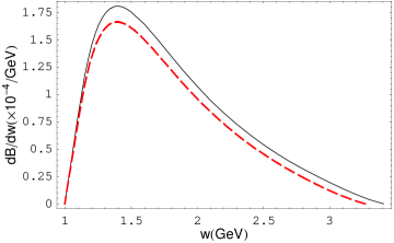
Figure 2: The kaon pair invariant mass spectra of $\bar{B}^{0}\to D^{+}K^{-}K^{0}$ (solid line) and $\bar{B}^{0}\to D^{*+}K^{-}K^{0}$ (dashed line).

From Table 1, the theoretical predictions of branching ratios are consistent with the experimental data. For the ratio $r_{K^{-}K^{0}}$, it needs further tests. The momentum spectra plotted in Fig. 2 shows a similar momentum distribution for pseudoscalar and vector D mesons. The fraction comes from the range $w<1.5{\rm GeV}$ is about 35% which is not sufficient to guarantee the validity of the collinear approximation. Note that this numerical result is based on our insufficient information of the $K^{-}K^{0}$ weak vector current form factor. From physical considerations, the $K^{-}K^{0}$ form factor in the small invariant mass region is likely to be enhanced by the resonance contribution or soft re-scattering effects. The expected momentum spectra should be more concentrated in the mass region close to the threshold where the two kaons are collinear. This conjecture is reinforced by the experimental measurement that the fraction of $B^{-}\to D^{0}K^{-}K^{0}$ signal events in the invariant mass range $w<1.3{\rm GeV}$ is 55%. The best fit $K^{-}K^{0}$ form factor in CHST does not satisfy this criterion. If the future experiment observes that most of the contribution comes from the small invariant mass region, such as $w<1.5{\rm GeV}$, it will provide a strong support of our conjecture. Furthermore, we suggest to extract the $K^{-}K^{0}$ weak form factor directly from the momentum spectrum of $\bar{B}^{0}\to D^{+}K^{-}K^{0}$.

One conclusion can be obtained from the QCD factorization is that the power correction is proportional to $w/m_{b}$. So, the factorization is only applicable for the invariant mass smaller than 2${\rm GeV}$. For three body baryonic B decays, the threshold energy of two baryons is higher than 2${\rm GeV}$. So, three body baryonic B decays is at the margin of the factorization method. Although the $K^{-}K^{0}$ form factor is not known accurately at present, we give a crude estimate about the theoretical errors in $\bar{B}^{0}\to D^{(*)+}K^{-}K^{0}$ decays based on power counting. The next-to-leading power correction at the amplitude level is proportional to $\frac{2m_{K}}{m_{B}}$, which is about $20\%$. At the decay rate level, the theoretical accuracy within $40\%$ is possible to be accessible in QCD factorization method. This accuracy is not as good as that in $B\to D\pi$, but it is still important in explaining the experimental data and understanding the hadronic physics of three body decays.

The principle that the hadron pair produced through quark-antiquark pair can be applied to other three body B-meson decays, such as $D\pi\pi$, $\pi\pi K$ etc. For these processes, more generalized distribution amplitudes are required. Some studies of using GDAs (or called two-hadron distribution amplitudes) in B decays have been considered in MCL . The detailed exploration of this subject is also required.

We would like to thank H. Li and C. Chua for many valuable discussions. This work is partly supported by Grant FPA/2002-0612 of the Spanish Ministry of Science and Technology, National Science Council of R.O.C. under Grant No. NSC 91-2816-M-001-0012-6.

References

- (1) A. Drutskoy et al. [Belle Collaboration], Phys. Lett. B 542, 171 (2002).
- (2) C. Chua, W. Hou, S. Shiau and S. Tsai, arXiv: hep-ph/0209164.
- (3) M. Bauer, B. Stech and M. Wirbel, Z. Phys. C 34, 103 (1987).
- (4) J. Bjorken, Nucl. Phys. B (Proc. Suppl.) 11, 325 (1989).
- (5) M. Beneke, G. Buchalla, M. Neubert and C. Sachrajda, Nucl. Phys. B 591, 313 (2000);
- (6) S. Brodsky and G. Lepage, Phys. Rev. D22, 2157 (1980).
- (7) C. Bauer, D. Pirjol and I. Stewart, Phys. Rev. Lett. 87, 201806 (2001)
- (8) M. Diehl, T. Gousset, B. Pire and O. Teryaev, Phys. Rev. Lett. 81, 1782 (1998).
- (9) X. Ji, Phys. Rev. Lett. 78, 610-613 (1997); D. Muller, D. Robaschik, B. Geyer, F.M. Dittes and J. Horejsi, Fortsch.Phys 42, 101 (1994) or arXiv: hep-ph/9812448.
- (10) C.W. Bauer, D. Pirjol, I.W. Stewart, Phys. Rev. D65, 054022 2002.
- (11) C.W. Bauer, S. Fleming, D. Pirjol and I.W. Stewart, Phys. Rev. D63, 114020 (2001).
- (12) M. Beneke, A.P. Chapovsky, M. Diehl and T. Feldmann, Nucl. Phys. B 643, 431 (2002).
- (13) S.W. Bosch, R.J. Hill (SLAC), B.O. Lange and M. Neubert, Phys. Rev. D67, 094014 (2003).
- (14) Z. Wei, Phys. Lett. B 586, 282-290 (2004); Z. Wei, arXiv: hep-ph/0403069.
- (15) S. Brodsky and G. Lepage, Phys. Lett. B 87, 359 (1979); A. Efremov and A. Radyushkin, Phys. Lett. B 94, 245 (1980).
- (16) M. Polyakov, Nucl. Phys. B 555, 231 (1999).
- (17) M. Maul, Eur. Phys. J. C 21, 115 (2001); C. Chen and H. Li, arXiv: hep-ph/0209043.