UCB-PTH-03-01

LBNL-52029

FERMILAB-PUB-03/017-T

Bulk Gauge Fields in Warped Space and
Localized Supersymmetry Breaking

Z. Chacko^a,b,c, and Eduardo Pontón^d,e

^aDepartment of Physics, University of California, Berkeley, CA 94720, USA
^b Theoretical Physics Group, Lawrence Berkeley National Laboratory,
Berkeley, CA 94720, USA
^d Fermi National Accelerator Laboratory, P.O. Box 500, Batavia, IL 60510, USA

^cemail: zchacko@thsrv.lbl.gov     ^eemail: eponton@fnal.gov

Abstract

We consider five dimensional supersymmetric warped scenarios in which the Standard Model quark and lepton fields are localized on the ultraviolet brane, while the Standard Model gauge fields propagate in the bulk. Supersymmetry is assumed to be broken on the infrared brane. The relative sizes of supersymmetry breaking effects are found to depend on the hierarchy between the infrared scale and the weak scale. If the infrared scale is much larger than the weak scale the leading supersymmetry breaking effect on the visible brane is given by gaugino mediation. The gaugino masses at the weak scale are proportional to the square of the corresponding gauge coupling, while the dominant contribution to the scalar masses arises from logarithmically enhanced radiative effects involving the gaugino mass that are cutoff at the infrared scale. While the LSP is the gravitino, the NLSP which is the stau is stable on collider time scales. If however the infrared scale is close to the weak scale then the effects of hard supersymmetry breaking operators on the scalar masses can become comparable to those from gaugino mediation. These operators alter the relative strengths of the couplings of gauge bosons and gauginos to matter, and give loop contributions to the scalar masses that are also cutoff at the infrared scale. The gaugino masses, while exhibiting a more complicated dependence on the corresponding gauge coupling, remain hierarchical and become proportional to the corresponding gauge coupling in the limit of strong supersymmetry breaking. The scalar masses are finite and a loop factor smaller than the gaugino masses. The LSP remains the gravitino.

1 Introduction

Supersymmetry provides an attractive framework for solving the hierarchy problem but it introduces several naturalness puzzles of its own. In particular it is not clear why the squark masses should be flavor diagonal. One class of natural solutions arises in theories where the quark and lepton fields are localized on a ‘3-brane’ in extra dimensions and the hidden sector field which breaks supersymmetry is localized on another spatially separated 3-brane. In such a framework contact terms between the visible and hidden fields in the four dimensional effective theory generated by the exchange of bulk states with masses much larger than the inverse brane spacing are exponentially small [1]. The dominant contribution to the soft scalar masses will then be generated by the exchange of the light states in the bulk. If the couplings of these light states are flavor blind the scalar masses will be flavor diagonal. The spectrum of the superparticles obtained for various choices of the bulk states has been extensively investigated in the literature for the case when the space between the branes is flat (unwarped). When the higher dimensional supergravity multiplet is the only light bulk state then the leading contribution to the soft scalar masses is given by anomaly mediation [1, 3]. If the MSSM gauge fields are also in the bulk and couple directly to the supersymmetry breaking sector then the leading contribution to the soft scalar masses arises from gaugino mediation [4, 5] provided the hidden sector field which breaks supersymmetry is a singlet. If this field is not a singlet then other effects such as radion mediation [6] and gaugino assisted anomaly mediation [7] dominate. In each of these cases a characteristic and interesting spectrum of flavor diagonal soft masses is obtained.

In this paper we consider contributions to the superparticle masses when the space between the branes is not flat, but warped as in RS1 [2]. We have two major motivations for considering supersymmetry breaking effects in these spaces. Firstly, since any realistic brane is expected to have a tension some degree of warping seems inevitable, and since the effect of warping on the spectrum can be significant it should be taken into account. Secondly, as we establish in this paper, physics on any one of the branes is screened from symmetry breaking effects on the other brane above the compactification scale, which is of order the mass of the lightest Kaluza-Klein particle. The potentially large hierarchy between the cutoff of the theory and the compactification scale (which is in contrast to theories with a flat extra dimension) can then be used to address other naturalness problems of the Standard Model.

In our framework the Standard Model quarks and leptons are localized to the brane where the warp factor is large (the ‘UV brane’) while supersymmetry is broken on the brane where the warp factor is small (the ‘IR brane’). The Standard Model gauge fields are in the bulk [10, 11] and couple directly to the supersymmetry breaking sector, while the field which breaks supersymmetry is a singlet. We further assume that the radion is stabilized supersymmetrically so that its F component is zero. Gauge coupling constant evolution in these models has been established as logarithmic [12]–[22]. Therefore, in order to explain the observed unification of coupling constants, we further restrict ourselves to the case where the theory respects a grand unifying symmetry at very short distances that is broken by the Higgs mechanism on the UV brane at a scale of about $10^{16}$ GeV.

In general, we find that the relative sizes of various supersymmetry breaking effects depend on the warp factor and therefore the spectrum differs significantly from that of the corresponding theory in flat space. If the warp factor is sufficiently small that the compactification scale is hierarchically larger than the weak scale then the dominant contribution to the Standard Model superpartner masses arises from gaugino mediation. Here the gaugino masses arise from a nonrenormalizable contact operator on the IR brane and are proportional to the square of the corresponding gauge coupling. The scalar masses are finite and generated radiatively through loops involving the gaugino mass. These loops are cutoff at the compactification scale so that while the scalar masses are loop suppressed with respect to the gaugino masses they are logarithmically enhanced by the ratio of the compactification scale to the weak scale. We determine the spectra for several different values of the compactification scale. In these models the LSP is the gravitino, while the NLSP is the stau. Since the scale of supersymmetry breaking is relatively high, the stau is stable on collider time scales. Some degree of fine tuning is required to obtain a viable spectrum, in part because of the bound on the Higgs mass and in part because of the bound on the stau mass.

If the warp factor is sufficiently large that the compactification scale is close to the weak scale then contributions to the scalar masses from loop diagrams involving hard supersymmetry breaking operators can become large and comparable to the effects of the gaugino mediation. The effect of these hard breaking operators, which were previously considered in [7], is to alter the relative coupling of gauge bosons and gauginos to matter. While the new loop diagrams contributing to the scalar masses are finite and cutoff at the compactification scale like the gaugino mediated graphs, their contributions are no longer related to the gaugino masses, and further, their sign is not fixed. The dependence of the gaugino masses on the corresponding gauge coupling is also more complicated since the effect of repulsion of the gaugino wave function from the IR brane is in general no longer negligible. The gaugino masses remain hierarchical and in the limit of strong supersymmetry breaking become proportional to the corresponding gauge coupling. Supersymmetry breaking in this limit where the compactification scale is close to the weak scale has been considered previously [23, 24, 25, 26]. However these authors did not take into account the effects of brane localized kinetic terms on the soft masses. In models where the grand unifying symmetry is broken on the UV brane, either by the Higgs mechanism or by boundary conditions, these effects cannot be neglected since the difference in the four dimensional gauge couplings of SU(3), SU(2) and U(1) arises from such terms. As a result our conclusions differ from theirs in significant details.

This paper is organized as follows. In section 2 we describe the general properties of fields propagating in an AdS background. We also address some aspects of the quantum theory and the physics of localized gauge symmetry breaking. In section 3 we turn our attention to localized supersymmetry (SUSY) breaking and determine the gaugino masses in various limits. In section 4 we discuss the phenomenology of the present class of models and in section 5 we give our conclusions. We summarize various technical details in the appendices. In appendix A we derive the gauge boson propagator in the presence of localized gauge symmetry breaking, and we present its behavior in various energy regimes. In appendix B we derive the gaugino propagator including the breaking of the gauge symmetry. Finally, in appendix C we derive the lightest gaugino mass when SUSY breaking is localized on the infrared brane and there are brane localized (gauge boson and) gaugino kinetic terms on the UV brane.

2 The Framework

We now consider a concrete five dimensional scenario. We employ a coordinate system $x^{M}$ where $M$ runs from 0 to 3 and 5. The fifth dimension $x^{5}=y$ is compactified on the interval $0\leq y\leq L$, which can be thought as arising from the orbifold $S^{1}/Z_{2}$. There are 3-branes at the orbifold fixed points $y=0$ and $y=L$. The space is warped and the Standard Model quarks and leptons are localized on the brane at $y=0$ where the warp factor is large. Supersymmetry is assumed to be broken on the brane where the warp factor is small. The metric is given by the line element

$$ds^{2}=e^{-2\sigma}\eta_{\mu\nu}dx^{\mu}dx^{\nu}+dy^{2}~{}.$$ (1)

Here the $x^{\mu}$, where $\mu$ runs from 0 to 3, parametrize our usual four spacetime dimensions, $\eta_{\mu\nu}={\rm{diag}}(-1,1,1,1)$, and $\sigma=k\left|y\right|$, where $k$ is the AdS curvature and is related to the four dimensional Planck scale $M_{4}$ and the five dimensional Planck scale $M_{5}$ by

$$M_{4}^{2}=\frac{M_{5}^{3}}{2k}\left(1-e^{-2kL}\right)\simeq\frac{M_{5}^{3}}{2k}~{},$$ (2)

where the second equality holds when the warping is significant.

The gauge fields of the Standard Model are assumed to propagate in the bulk. An on shell vector multiplet in five dimensional ${\cal{N}}=1$ supergravity consists of a gauge field $A_{M}$, a pair of symplectic Majorana spinors $\lambda^{i}$, with $i=1,2$, and a real scalar $\Sigma$ which transforms in the adjoint representation. The bosonic part of the higher dimensional gauge field Lagrangian takes the form

$${\cal{L}}_{b}=-\frac{1}{g_{5}^{2}}\left[\frac{1}{4}F_{MN}F^{MN}+\frac{1}{2}D_{M}\Sigma\;D^{M}\Sigma+\left(\sigma^{\prime\prime}-2k^{2}\right)\Sigma^{2}\right]~{},$$ (3)

where $\sigma^{\prime\prime}=2k\left[\delta(y)-\delta(y-L)\right]$. The fermionic part takes the form

$${\cal{L}}_{f}=-\frac{i}{2g_{5}^{2}}\left[\bar{\lambda}^{i}\Gamma^{M}D_{M}\lambda^{i}+\frac{1}{2}\sigma^{\prime}\bar{\lambda}^{i}\left(\sigma^{3}\right)^{ij}\lambda^{j}\right]~{},$$ (4)

where $D_{M}$ is a covariant derivative with respect to both general coordinate and gauge transformations. The vielbein factors necessary to write the spinor action in curved space are implicit in Eq. (4). In addition to the interactions above, additional brane localized terms that preserve $N=1$ supersymmetry are also possible, but we postpone their consideration until the next subsection.

We demand that $A_{\mu}$ and $\lambda^{1}_{L}$ are even while $\Sigma$ and $\lambda^{2}_{L}$ are odd. Then the even fields each have a massless mode with the following $y$ dependence:

$$A_{\mu}\left(x,y\right) = \frac{1}{\sqrt{L}}A_{\mu}^{\left(0\right)}\left(x\right)+\cdots$$ (5)

$$\lambda^{1}_{L}\left(x,y\right) = \frac{e^{3\sigma/2}}{\sqrt{L}}\lambda^{1\;\left(0\right)}_{L}\left(x\right)+\cdots$$ (6)

In the previous theory, an approximate expression for the masses $m_{n}$ of the Kaluza Klein (KK) states can be obtained in the limit that $k\gg m_{n}$ and $kL\gg 1$:

$$m_{n}\approx\left(n-\frac{1}{4}\right)\pi ke^{-kL}~{}.$$ (7)

This shows that the KK masses are of order $M_{c}=k\,e^{-kL}$, which we will call the compactification scale.

In order to make physical predictions for low energy observables we will need a consistent framework for quantum field theory in warped space. It has been shown by Goldberger and Rothstein [16] that a setup in which the parameters of the Lagrangian are defined in terms of correlators with external points localized on the Planck brane is one such consistent framework. In particular this allows the renormalization group evolution of the theory from short distances down to the compactification scale, where it can be matched onto a four dimensional effective theory. This is the approach we shall be using. Its consistency relies on the the general properties of the bulk tree-level propagators. In fact, all perturbative calculations can be done, in principle, once the higher dimensional propagators are known. Even though, in practice, it is technically simpler to do calculations in terms of KK modes, an understanding of how the higher dimensional calculation would proceed provides considerable physical insight.

2.1 General Properties of Propagators in AdS backgrounds

To illustrate the physical properties of propagators in the AdS background Eq. (1), we consider the tree-level gauge boson propagator. The action has the following form:

$$\int_{0}^{L}d^{4}\!x\,dy\left\{-\frac{1}{4g_{5}^{2}}\sqrt{-G}\,F_{MN}F^{MN}+2\delta\left(y\right)\sqrt{-G_{\rm{ind}}}\left[{\cal{L}}_{UV}-\frac{1}{4g_{UV}^{2}}F_{\mu\nu}F^{\mu\nu}\right]\right.$$

$$\left.\hskip 116.65646pt\mbox{}+2\delta\left(y-L\right)\sqrt{-G_{\rm{ind}}}\left[{\cal{L}}_{IR}-\frac{1}{4g_{IR}^{2}}F_{\mu\nu}F^{\mu\nu}\right]\right\}~{},$$ (8)

where ${\cal{L}}_{UV}$ and ${\cal{L}}_{IR}$ describe brane localized fields that may be charged under the gauge group. We also include brane localized gauge kinetic terms, which are expected to be induced radiatively. For simplicity, in this section we will assume that they can be treated perturbatively (see [29, 30] for a discussion of their effects when they are not small.)

When calculating the propagator, it is convenient to work in four-dimensional momentum space, as defined by

$$G(y;p)=\int\!d^{4}x\,e^{i\eta_{\mu\nu}p^{\mu}x^{\nu}}G(x,y)~{}.$$ (9)

Keeping the $y$ dependence makes the locality properties along the fifth dimension explicit. The four-dimensional momentum $p$, as defined in Eq. (9), is conserved in physical processes in the background Eq. (1). Nevertheless, it is important to keep in mind that $p^{\mu}$ is not necessarily the physical momentum of the propagating field as measured by an observer standing at an arbitrary point in the bulk $y$. For example, such an observer would measure an energy (frequency) $E_{\rm{phys}}=1/\Delta\tau=e^{ky}/\Delta x^{0}=e^{ky}p^{0}$, where $\tau$ is proper time and $x^{0}$ is the time coordinate used in Eq. (1), which is conjugate to $p^{0}$. In the following, any statements regarding energy scales will refer to the values of the “coordinate” momentum $p$, and therefore they should be understood as scales measured by UV observers.

We start with the propagator in the absence of gauge symmetry breaking or brane localized gauge kinetic terms, which has been calculated elsewhere (see, e.g. [24]). It is useful to consider first the case where the UV and IR boundaries are sent to infinity, so that the background is pure AdS. Neglecting the tensor structure and working in Euclidean space, the propagator evaluated at coincident points $y=y^{\prime}$ exhibits a remarkably simple behavior (see appendix A)

$$G_{p}(y,y)\sim-\frac{g_{5}^{2}}{2}\left\{\begin{array}[]{ll}\frac{e^{ky}}{p}&\vspace{2mm}\hskip 28.45274pt{\rm{for}}\;\;p\gg k\,e^{-ky}\\ \frac{2k}{p^{2}\ln(2k/p)}&\hskip 28.45274pt{\rm{for}}\;\;p\ll k\,e^{-ky}\end{array}\right.$$ (10)

We note that for sufficiently low energies, the propagator exhibits a four-dimensional scaling $\sim 1/p^{2}$, up to a logarithm. We stress that this is the case even before compactification. This property is intimately related to the AdS/CFT conjecture, which states that the five-dimensional theory is equivalent to a four-dimensional conformal field theory (CFT). The logarithm that appears for energies below $k\,e^{-ky}$ is sometimes described as a tree-level “running” of the gauge coupling and corresponds, in the four-dimensional dual picture, to CFT loop effects. We also see that $G_{p}(y,y)$ changes from a four-dimensional ($\sim 1/p^{2}$) to a five-dimensional ($\sim 1/p$) behavior at a scale $p\sim k\,e^{-ky}$. The onset of the higher dimensional scaling indicates that, for localized observers at $y$, the theory ceases to be predictive when the external 4-d momenta are much larger than $k\,e^{-ky}$. As emphasized in [16], the breakdown of the theory for external $p\gg k\,e^{-ky}$ is already apparent when considering tree-level insertions of higher dimension operators localized at $y$, which give contributions proportional to powers of $p/(ke^{-ky})$. Therefore, the theory defined by Eq. (2.1) should be understood as an effective theory with a $y$-dependent cutoff $\Lambda\,e^{-ky}$ on $p$, for some constant $\Lambda\begin{array}[]{c}\sim\vspace{-21pt}\\ >\end{array}k$.

Now we bring in the UV and IR boundaries. The asymptotic behavior given in Eq. (10) is modified in the following manner. The UV boundary affects only the high energy behavior of the propagator when evaluated at (or very close to) $y=0$: in this case the propagator is twice the result given in Eq. (10). The IR brane, on the other hand, changes only the low energy regime, for all $y$. One finds that for $p\ll k\,e^{-kL}$ the $\ln(2k/p)$ factor should be replaced by $kL$. Thus, the tree-level “running” stops at about the compactification scale $k\,e^{-kL}$.

One may wonder if a theory with a $y$-dependent cutoff can be used to make predictions at all, since even if one is only interested in calculating observables at a fixed position $y$, say on one of the orbifold fixed points, at some energy scale $p\ll k\,e^{-ky}$, such observables can receive contributions from other points in the bulk, where the local cutoff is lower than the relevant external momentum $p$. Such contributions are simply not calculable within the framework of the five-dimensional theory. To illustrate this, consider the contribution to UV brane observables from the following tower of operators localized on the IR brane:

$${\cal{L}}_{IR}\supset\sum_{n}c_{n}F_{\mu\nu}\Box^{n}F^{\mu\nu}~{},$$ (11)

where $\Box=G_{\rm{ind}}^{\mu\nu}\partial_{\mu}\partial_{\nu}=e^{2kL}\eta^{\mu\nu}\partial_{\mu}\partial_{\nu}$. The $n=0$ term corresponds to the IR brane localized gauge kinetic term that we wrote in Eq. (2.1), but in general we expect all the operators in Eq. (11) (and many other) to be present in the effective theory. Writing the coefficients of these higher dimension operators as $c_{n}=\hat{c}_{n}/M_{5}^{2n}$, where the $\hat{c}_{n}$ are dimensionless, we see that treating these operators perturbatively gives a contribution proportional to $\sum_{n}\hat{c}_{n}[p/(M_{5}\,e^{-kL})]^{2n}$. This shows that for $p\begin{array}[]{c}\sim\vspace{-21pt}\\ >\end{array}M_{5}\,e^{-kL}$ the effective theory breaks down. In spite of this observation, one should not necessarily conclude that the UV observables are not calculable when $M_{5}\,e^{-kL}\ll p\ll M_{5}$. One may see this by considering the tree-level propagator for non-coincident points $y\neq y^{\prime}$. Assuming that $y<y^{\prime}$, one finds

$$G_{p}(y,y^{\prime}) \sim -\frac{g_{5}^{2}k}{p^{2}\ln(2k/p)}\,\sqrt{\frac{\pi p}{2k}}\,e^{\frac{1}{2}ky^{\prime}}e^{-\frac{p}{k}e^{ky^{\prime}}}\hskip 22.76219pt{\rm{for}}\;\;k\,e^{-ky^{\prime}}\ll p\ll k\,e^{-ky}~{},$$

which exhibits a huge exponential suppression $e^{-\frac{p}{k}e^{ky^{\prime}}}$. This suggests that, whatever the physics at $y^{\prime}$ for energies much larger than the local cutoff $M_{5}\,e^{-ky^{\prime}}$ is, its effect on the physics at $y$ is exponentially suppressed and therefore unimportant. In particular, we do not expect contributions from short distance physics at $y^{\prime}$ to overcome the exponentially small probability for a gauge field to propagate there and back.

2.2 Quantum Field Theories in a slice of AdS

We now explain how quantum field theories can be formulated in warped spaces in terms of propagators with external legs on the Planck brane. Our discussion closely follows that of Goldberger and Rothstein [16]. For simplicity the theory we will be considering is a (non-supersymmetric) bulk U(1) gauge theory with fermionic matter localized on the UV and IR branes. This will suffice to illustrate our framework. The Lagrangian takes the form of Eq. (2.1) with ${\cal{L}_{UV}}$ and ${\cal{L}_{IR}}$ given by

$${\cal{L}}_{I}=\bar{\psi}_{I}\left(i\Gamma^{\mu}\partial_{\mu}-m_{I}\right){\psi}_{I}\hskip 28.45274ptI=UV,IR$$ (12)

Our regularization scheme involves dimensional regularization with momentum subtraction. Although this scheme is mass dependent it has the advantage that the decoupling of heavy states occurs automatically, without the necessity to match and run [31]. Since the cutoff for physics on the UV brane is of order $M_{5}$, the parameters of the Lagrangian ${\cal{L}}_{UV}$ on the UV brane can be defined at any subtraction point $\mu$ less than this. This is also true for the parameters of the bulk Lagrangian. However since the cutoff on the IR brane is of order $M_{5}\,e^{-kL}$ the parameters of the Lagrangian ${\cal{L}}_{IR}$ on the IR brane cannot be defined at any subtraction point higher than this. Nevertheless correlators with external legs on the UV brane and four momenta much larger than the cutoff on the IR brane can still be calculated up to exponentially small corrections. This is because, as we saw in the previous subsection, a propagator from the UV brane to any point in the bulk where the four momentum is larger than the local cutoff dies away exponentially quickly.

It is possible to renormalization group evolve the parameters of the Lagrangian on the UV brane ${\cal{L}}_{UV}$ and the bulk Lagrangian from $\mu$ of order $M_{5}$ down to the compactification scale $k\,e^{-kL}$. Similarly the parameters of the Lagrangian on the IR brane can be evolved from $\mu$ of order $M_{5}\,e^{-kL}$ down to the compactification scale. The complete higher dimensional Lagrangian can then be matched on to the four dimensional effective theory. Below we illustrate this procedure for the U(1) theory.

In order to obtain the dependence of the gauge coupling constant on the renormalization scale, we consider the quantum corrections to the two-point correlator for gauge fields with external points localized on the UV brane. For a U(1) gauge theory the corrections to the gauge coupling constant from renormalization of the vertex function and the two-point functions of the fermions can be made to cancel by the Ward-Takahashi identity. The corrections to the gauge field two point correlator arise from fermionic loops of the form below which are familiar from four dimensions. Considering first the correction from the fermionic loop on the UV brane alone we find

$$G_{\mu\nu}\left(0,0;p\right)\rightarrow G_{\mu\nu}\left(0,0;p\right)+G_{\mu\alpha}\left(0,0;p\right)\left[p^{2}\eta^{\alpha\beta}-p^{\alpha}p^{\beta}\right]i\Pi(p^{2})G_{\beta\nu}\left(0,0;p\right)~{},$$ (13)

where the gauge boson propagator $G_{\mu\nu}$ is related to the $G_{p}$ of the previous section by Eq. (45) of appendix A, and $\Pi(p^{2})$ must be regulated. We regulate this by momentum subtraction at a scale $p^{2}=\mu^{2}$, which is spacelike due to the signature implicit in the line element Eq. (1). Then $\Pi(p^{2})\rightarrow\Pi(p^{2})-\Pi\left(\mu^{2}\right)$. After regularization,

$$\Pi(p^{2})=-\frac{1}{2\pi^{2}}\int_{0}^{1}d\;x\;x\left(1-x\right){\rm log}\left[\frac{m_{UV}^{2}+x\left(1-x\right)\mu^{2}}{m_{UV}^{2}+x\left(1-x\right)p^{2}}\right]~{}.$$ (14)

Renormalization group flow is obtained by varying the scale $\mu$ above. The physical amplitudes remain invariant if the coefficient of the brane localized kinetic term $1/g_{UV}^{2}$ is varied so as to keep the complete two point correlator invariant. We obtain the following renormalization group equation for $1/g_{UV}^{2}$,

$$\frac{d\;g_{UV}}{d\;{\rm log}\mu}=\frac{g_{UV}^{3}}{2\pi^{2}}\int_{0}^{1}dx\;\mu^{2}\frac{x^{2}\left(1-x\right)^{2}}{m_{UV}^{2}+x\left(1-x\right)\mu^{2}}$$ (15)

This renormalization group equation is valid from the scale $M_{5}$ down to the compactification scale. For $\mu^{2}\gg m_{UV}^{2}$ we see that the renormalization group evolution of the brane localized kinetic term is the familiar one for QED in four dimensions, while for $\mu^{2}\ll m_{UV}^{2}$ the beta function tends to zero. Thus in this mass dependent renormalization scheme the decoupling of heavy modes is occurring automatically. This is the primary advantage of this scheme.

We now turn to the corrections to the two-point correlator from the IR brane. The fermionic loop on the IR brane leads to

$$G_{\mu\nu}\left(0,0;p\right)\rightarrow G_{\mu\nu}\left(0,0;p\right)+G_{\mu\alpha}\left(0,L;p\right)\left[p^{2}\eta^{\alpha\beta}-p^{\alpha}p^{\beta}\right]i\Pi(p^{2})G_{\beta\nu}\left(L,0;p\right)~{}.$$ (16)

Once again $\Pi(p^{2})$ must be regulated. As before we regulate this by momentum subtraction at a scale $p^{2}=\mu^{2}$. After regularization,

$$\Pi(p^{2})=-\frac{1}{2\pi^{2}}\int_{0}^{1}d\;x\;x\left(1-x\right){\rm log}\left[\frac{m_{IR}^{2}\;e^{-2kL}+x\left(1-x\right)\mu^{2}}{m_{IR}^{2}\;e^{-2kL}+x\left(1-x\right)p^{2}}\right]~{}.$$ (17)

The requirement that the two point function be independent of the arbitrary scale $\mu$ leads once again to a renormalization group equation for the coefficient of the brane localized kinetic term on the IR brane.

$$\frac{d\;g_{IR}}{d\;{\rm log}\mu}=\frac{g_{IR}^{3}}{2\pi^{2}}\int_{0}^{1}dx\;\mu^{2}\frac{x^{2}\left(1-x\right)^{2}}{m_{IR}^{2}\;e^{-2kL}+x\left(1-x\right)\mu^{2}}$$ (18)

This renormalization group equation is valid from the cutoff on the IR brane $M_{5}\,e^{-kL}$ down to the compactification scale. We see that in this case the fermion decouples at a scale $m_{IR}\,e^{-kL}$. Far above this scale the beta function is the one familiar from QED, while far below this scale it tends to zero.

The four dimensional effective theory for this model is obtained by performing a Kaluza Klein decomposition of the higher dimensional theory and integrating over the extra dimension. Provided the renormalization scale $\mu$ at which the entire higher dimensional theory is defined is close to the compactification scale then tree level matching of the parameters will be accurate up to loop effects which are not logarithmically enhanced.

It is important to know whether the framework we have described above can be generalized to the cases when there are bulk fields transforming under the gauge group, and when the gauge group is non-Abelian. Goldberger and Rothstein [16] have shown that the parameters of a U(1) theory with a bulk scalar field charged under the gauge group can be renormalization group evolved using correlators with external legs on the UV brane. However non-Abelian gauge theories have yet to be examined using this framework. Nevertheless in the sections that follow we will assume that it is possible to do this and proceed.

Now consider a ‘GUT’ model consisting of a U(1)${}_{A}\times$ U(1)_B gauge theory. Each U(1) has a Dirac fermion transforming under it on each of the two branes. The GUT symmetry here is a $Z_{2}$ which interchanges the gauge fields and the fermions transforming under them. What we are interested in understanding is the effect on the parameters on the IR brane if the GUT symmetry is broken on the UV brane. This will be useful for our purposes later. Suppose that the GUT symmetry is explicitly broken on the UV brane so that $m_{UV;A}>m_{UV;B}$. However we see from the renormalization group equation for $g_{IR}$ that (at least to one loop order) $g_{IR;A}=g_{IR;B}$ even below the scale $m_{UV;A}$. However below this scale $g_{UV;A}\neq g_{UV;B}$ so that the U(1) gauge coupling strengths in the four dimensional effective theory will be different. Nevertheless we see from this that parameters on the IR brane are screened from effects of symmetry breaking on the UV brane above the compactification scale.

2.3 Effect of Localized Gauge Symmetry Breaking

Now we consider the effects of gauge symmetry breaking. We will restrict to the case where the breaking is due to the VEV of a Higgs field localized on the UV brane. Since we are interested in the case where the gauge symmetry is broken at a high scale $v\sim M_{GUT}\sim 10^{16}~{}\rm{GeV}$, the effects of $v$ must be included exactly in the propagator at tree-level. We leave the relevant details to appendix A, where the exact tree-level gauge boson propagator in $A_{5}=0$ gauge and four-dimensional unitary gauge is calculated. There, we also summarize the asymptotic forms of the resulting propagator in the various energy regimes. We base the present discussion on the asymptotic behavior of the propagator, which is physically more transparent. Referring to the propagator $G_{p}(y,y)$ defined in Eq. (45) of appendix A, we find that for the broken gauge bosons, and provided $g_{5}^{2}v^{2}\begin{array}[]{c}\,\sim\vspace{-21pt}\\ <\end{array}k$, its high energy behavior, $p\gg k\,e^{-ky}$, is unchanged compared to the unbroken case up to very small corrections (see Eqs. (52) and (53) of appendix A). Thus, if the VEV $v$ is responsible for the breaking of the gauge group G down to a subgroup H, observers at $y$ will see (at least at tree-level) the full symmetry G when probing energies above $k\,e^{-ky}$, a scale that is in general much lower than the naive scale of symmetry breaking of order $v$. Only for momenta $p\ll k\,e^{-ky}$ do observers at $y$ have a chance to see that the gauge symmetry is actually broken. In that energy regime and without making any assumptions about the size of $v$, we find (see Eqs. (55) and (56) of appendix A)

$$G_{p}(y,y)\sim-\frac{g_{5}^{2}}{2}\;\frac{2k+(e^{2ky}-1)\,g_{5}^{2}v^{2}}{p^{2}\ln(2k/p)+k\,g_{5}^{2}v^{2}}\hskip 28.45274ptk\,e^{-kL}\ll p\ll k\,e^{-ky}~{},$$ (19)

while

$$G_{p}(y,y)\sim-\frac{g_{5}^{2}}{2\,k}\;\frac{2k+(e^{2ky}-1)\,g_{5}^{2}v^{2}}{Lp^{2}+\,g_{5}^{2}v^{2}}\hskip 28.45274ptp\ll k\,e^{-kL}~{}.$$ (20)

We see again that Eq. (20) can be obtained from Eq. (19) by making the replacement $\ln(2k/p)\rightarrow kL$.

Specializing to the case of interest here, where $v\sim M_{\rm{GUT}}\sim k$, we note from Eq. (20) that at very low energies, $p\ll k\,e^{-kL}$, the UV propagator is

$$G_{p}(0,0)\sim-\frac{1}{v^{2}}~{}.$$ (21)

Therefore, when matter is localized on the UV brane, processes mediated by the broken gauge bosons, such as proton decay, are exactly as suppressed as in conventional four-dimensional theories. For IR localized observers, one finds instead

$$G_{p}(L,L)\sim-\frac{g_{5}^{2}}{2k}\,e^{2kL}\sim-\frac{g_{4}^{2}}{2k/L}\,e^{2kL}~{},$$ (22)

where $g_{4}^{2}=g_{5}^{2}/L$ is the four-dimensional gauge coupling of the unbroken gauge bosons. Thus, the broken gauge bosons appear to have a mass of order $(k/L)^{1/2}\,e^{-kL}$ from the point of view of IR observers. This is consistent with our previous observation that the broken gauge bosons behave like massless fields above the compactification scale $k\,e^{-kL}$.

The picture suggested by the above discussion is that all IR correlators will exhibit relations appropriate to the full symmetry group of the theory at energies somewhat larger than the compactification scale $k\,e^{-kL}$. The same would hold for the coefficients of operators localized on the IR brane. In order to make the above statement precise one has to go beyond the previous tree-level analysis and argue that loop effects will not modify this picture. We will consider this in a subsequent section. Nevertheless this is completely consistent with our results for the case of the discrete $Z_{2}$ symmetry in the previous subsection.

3 Localized Supersymmetry Breaking

We are considering a scenario where supersymmetry is broken on the infrared brane and supersymmetry breaking effects are transmitted to fields localized on the ultraviolet brane by the gauge multiplet in the bulk. However, the GUT symmetry is assumed to be broken on the ultraviolet brane, at a scale $M_{GUT}$ much higher than the compactification scale, which we denote by $M_{c}\equiv k\,e^{-kL}$. We must therefore be careful to take GUT symmetry breaking effects into account when computing the sparticle masses. The hierarchy of scales we are considering is $M_{5}\begin{array}[]{c}\sim\vspace{-21pt}\\ >\end{array}k\begin{array}[]{c}\sim\vspace{-21pt}\\ >\end{array}M_{GUT}\gg M_{c},\sqrt{F}$. At energy scales well above the GUT scale the Planck brane correlators of the theory will respect the GUT symmetry. Hence the parameters of the bulk Lagrangian and the parameters of the Lagrangian on the UV brane defined at a 4-d momentum scale $\mu>M_{GUT}$ will respect the GUT symmetry, and any divergences that arise at loop level can be removed by adding counterterms that respect this symmetry. However the parameters on the IR brane cannot be defined at a scale so much higher than the cutoff on the IR brane. Nevertheless the results of the previous section suggest that they can consistently be defined as GUT symmetric at a scale close to the cutoff on the IR brane $M_{5}\,e^{-kL}$. This is because physics on the IR brane is screened from the effects of GUT symmetry breaking on the UV brane above the compactification scale.

At 4-d momentum scales lower than the GUT scale the Planck brane correlators will in general no longer respect the GUT symmetry, corresponding to the fact that the parameters of the Lagrangian on the UV brane are no longer GUT symmetric. Our approach will be to evolve the higher dimensional Lagrangian from the GUT scale to a scale $\mu\approx M_{c}$ and then match on to the four dimensional effective theory at tree level. Any matching corrections to our expressions will then be loop suppressed and in particular, they will not be enhanced by the logarithm of $M_{GUT}/M_{c}$.

We begin by investigating the effects of GUT symmetry breaking on the supersymmetric terms in the Lagrangian. Consider the form of the Lagrangian for the gauginos. At 4-d scales above the GUT scale the supersymmetric part of the action has a bulk contribution

$$-\frac{1}{g_{5}^{2}}\int_{0}^{L}d^{4}\!x\,dy\sqrt{-G}\;\sum_{A\in SU(5)}\left[\frac{i}{2}\bar{\lambda}^{iA}\Gamma^{M}D_{M}\lambda^{iA}+\frac{i}{4}\sigma^{\prime}\bar{\lambda}^{iA}\left(\sigma_{3}\right)^{ij}\lambda^{jA}\right]~{},$$ (23)

and a brane localized contribution

$$-\frac{1}{g_{UV}^{2}}\int_{0}^{L}d^{4}\!x\,dy\sqrt{-G_{\rm{ind}}}\;2\delta\left(y\right)\sum_{A\in SU(5)}\left[i\bar{\lambda}^{1A}\Gamma^{\mu}D_{\mu}P_{L}\lambda^{1A}\right]$$ (24)

on the UV brane, where we inserted the chirality projector $P_{L}$ so that only the left-handed components of the bulk gaugino appear in the brane term.

At energy scales below the GUT scale the form of the action changes. While the forms of the bulk action Eq. (23) and the IR brane action Eq. (26) remain the same, the contribution to the action from the UV brane where the GUT symmetry is broken now takes the form

$$-\int_{0}^{L}d^{4}\!x\,dy\sqrt{-G_{\rm{ind}}}\;2\delta\left(y-L\right)\sum_{A\in SU(5)}\left[\frac{1}{g_{UV,A}^{2}}\,i\,\bar{\lambda}^{1A}\Gamma^{\mu}D_{\mu}P_{L}\lambda^{1A}\right]~{},$$ (25)

where because of GUT symmetry breaking $g_{UV,A}^{2}$ is in general not the same for SU(3), SU(2), U(1) and SU(5)/[SU$(3)\times$ SU(2)$\times$U(1)].

The kinetic terms for the gaugino on the IR brane are defined at the scale $M_{5}\,e^{-kL}$ and take the SU(5) symmetric form

$$-\frac{1}{g_{IR}^{2}}\int_{0}^{L}d^{4}\!x\,dy\sqrt{-G_{\rm{ind}}}\;2\delta\left(y-L\right)\sum_{A\in SU(5)}\,i\,\bar{\lambda}^{1A}\Gamma^{\mu}D_{\mu}P_{L}\lambda^{1A}$$ (26)

Renormalization group evolving this down to $M_{c}$ does not alter the SU(5) symmetric form.

In order to obtain the four dimensional effective action we determine the form of the complete higher dimensional action at a scale close to $M_{c}$ and after performing a Kaluza- Klein decomposition we then integrate over the extra dimension. Since the SU(5)/[SU$(3)\times$SU(2)$\times$U(1)] gauginos all have masses of order the compactification scale or higher the only surviving degrees of freedom are the zero modes of the SU(3), SU(2) and U(1) gauginos. The four dimensional effective theory for the zero mode gauginos is now the one familiar from four dimensions:

$$-\int d^{4}x\sqrt{-g}\sum_{A\in SU(3),SU(2),U(1)}\frac{1}{g_{A}^{2}}\,\frac{i}{2}\,\bar{\lambda}_{L}^{A}{\Gamma}^{\mu}{D}_{\mu}\lambda_{L}^{A}~{},$$ (27)

where now $\lambda_{L}^{A}=(\lambda^{1}_{\alpha},\bar{\lambda}^{1\dot{\alpha}})$ is a four component Majorana spinor built from the even components of the original symplectic Majorana pair (all other components get masses of the order of the compactification scale). Also, the relation between the 4-dimensional gauge coupling $g_{A}^{2}$ and the fundamental parameters in the theory takes the form

$$\frac{1}{g_{A}^{2}}=\frac{L}{g_{5}^{2}}+\frac{1}{g_{IR}^{2}}+\frac{1}{g_{UV,A}^{2}}~{},$$ (28)

where the first two terms are essentially GUT symmetric, but the last one contains nonuniversal logarithms from loop effects.

We now turn our attention to supersymmetry breaking terms. Consider the effect of the following supersymmetry breaking term localized on the infrared brane.

$$\int_{0}^{L}d^{4}\!x\,dy\sqrt{-G_{\rm{ind}}}\;2\delta\left(y-L\right)\sum_{A\in SU(5)}\left\{\frac{1}{8}\int d^{4}\theta\frac{X^{\dagger}X}{M_{5}^{4}}W^{\alpha A}D^{2}W_{\alpha}^{A}+H.c.\right\}~{},$$ (29)

where $X$ is the hidden sector superfield that breaks supersymmetry ($F_{X}\neq 0$) and $W_{\alpha}^{A}=-i\lambda_{\alpha}^{1A}+\cdots$ is the field strength superfield constructed from the left-handed component of $\lambda^{1A}$. We follow the conventions of [32]. The effect of such a term is to alter the relative strengths of the couplings of the gauge boson and gaugino to matter. This contributes to the zero mode gaugino Lagrangian a term

$$-\int_{0}^{L}d^{4}\!x\,dy\sqrt{-G_{\rm{ind}}}\;2\delta\left(y-L\right)\sum_{A\in SU(5)}\frac{|F|^{2}}{M_{5}^{4}}\,\,\frac{i}{2}\,\bar{\lambda}_{L}^{A}\Gamma^{\mu}{D}_{\mu}\lambda_{L}^{A}~{},$$ (30)

where the four-component spinors $\lambda_{L}^{A}$ are defined as in Eq. (27), but keeping the full $y$-dependence. The arguments of the previous section suggest that this term is SU(5) symmetric at compactification scale $k\,e^{-kL}$. We now show that if the GUT symmetry is only broken on the UV brane loop corrections to this term from above the compactification scale do indeed respect the SU(5) symmetric form.

To determine the form of this term at the matching scale $M_{c}$ we consider the two point function for the gaugino in mixed position momentum space with four momentum of order the IR scale and the end points on the UV brane. We base our discussion in terms of the properties of the tree-level gaugino propagator. For example, we find that the propagator for the even spinor components, $G_{LL}^{A}\equiv P_{L}G^{A}P_{R}=\langle\lambda_{L}^{A}\overline{\lambda_{L}^{A}}\rangle$, is

$$G_{LL}^{A}(y,y^{\prime};p)=-iP_{L}\!\not{\!p}\,\,e^{\frac{3}{2}k(y+y^{\prime})}G_{p}^{A}(y,y^{\prime})\hskip 28.45274ptA\in SU(5)~{},$$ (31)

where $G_{p}^{A}(y,y^{\prime})$ is precisely the scalar part of the gauge boson propagator (see Eq (50) in appendix A), whose properties where discussed in Section 3. Equation (31) holds for the unbroken as well as for the broken fields. We provide the details of the derivation of the gaugino propagator in the presence of UV localized gauge symmetry breaking in appendix B, where we also give the exact expressions for $G_{RR}$, $G_{RL}$ and $G_{LR}$ (see Eqs. (95), (90) and (83)).

If we treat the operator Eq. (30) perturbatively, the UV brane two-point gaugino correlator receives an SU(5) symmetric tree-level contribution proportional to

$$G^{A}_{LL}\left(0,L;p\right)\left(\Gamma^{\alpha}p_{\alpha}\,\frac{|F|^{2}}{M_{5}^{4}}\,e^{-3kL}\right)G^{A}_{LL}\left(L,0;p\right)~{},$$ (32)

where the factor $e^{-3kL}$ comes from the determinant of the induced metric and the vielbein implicit in the contraction $\Gamma^{\mu}D_{\mu}$ (see Fig. 1 a). Now consider loop corrections with one insertion of Eq. (30). One of the contributions to the leading one-loop amplitude is shown in Fig. 1 b and has the form

$$\sum_{B,C\in SU(5)}\left(f^{ABC}\right)^{2}\int\frac{d^{4}q}{(2\pi)^{4}}\int_{0}^{L}dy^{\prime}\int_{0}^{L}dy^{\prime\prime}G^{A}_{LL}\left(0,y^{\prime};p\right)\Gamma^{\mu}G_{LL}^{C}\left(y^{\prime},L;p+q\right)$$ (33)

$$\mbox{}\times\left(\Gamma^{\alpha}p_{\alpha}\,\frac{|F|^{2}}{M_{5}^{4}}\,e^{-3kL}\right)G_{LL}^{C}\left(L,y^{\prime\prime};p+q\right)G^{B}_{\mu\nu}\left(y^{\prime},y^{\prime\prime};q\right)\Gamma^{\nu}G^{A}_{LL}\left(y^{\prime\prime},0;p\right)~{},$$

where $f^{ABC}$ are the structure constants of $SU(5)$.

                 

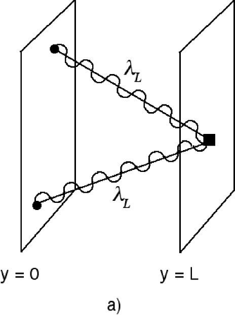
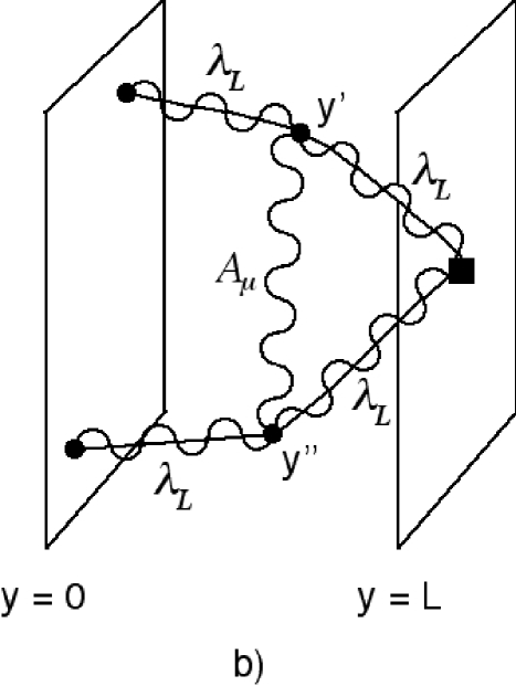
Figure 1: Contributions to the two-point gaugino correlator with end points on the UV brane from the operator Eq. (30), represented by a square, in the one insertion approximation. a) Tree-level and b) one of the 1-loop contributions.

This diagram is divergent for large loop momenta $q$ when the vertices $y^{\prime}$ and $y^{\prime\prime}$ become close to $L$. However the form of this divergence is SU(5) symmetric, since the forms of the relevant propagators for both the broken and unbroken generators are the same up to exponentially small differences when $q\gg k\,e^{-kL}$. From the forms of the propagators it can be further inferred that SU(5) violating corrections to the supersymmetry breaking term Eq. (30), if any, from loop momenta much higher than the IR scale are exponentially suppressed and therefore small. From this we conclude that the form of this parameter in the higher dimensional theory at a scale close to the matching scale is SU(5) symmetric and any corrections to this are loop suppressed and without any logarithmic enhancement. Based on this we argue that any supersymmetry breaking term localized on the IR brane will have an SU(5) symmetric form up to loop suppressed corrections at four dimensional momenta of order the compactification scale.

We now obtain an expression for the gaugino soft masses in the limit where the SUSY breaking scale is well below the compactification scale $M_{c}$. These arise from operators of the form

$$\int_{0}^{L}d^{4}\!x\,dy\sqrt{-G_{\rm{ind}}}\;2\delta\left(y-L\right)\sum_{A\in SU(5)}\frac{1}{2}\int d^{2}\theta\frac{\lambda X}{M_{5}}W^{\alpha A}W_{\alpha}^{A}~{},$$ (34)

localized on the hidden brane where supersymmetry is broken. Here $X$ is the hidden sector field which breaks supersymmetry, $\lambda$ is a coupling constant, and we are assuming that $F_{X}\neq 0$. From our previous discussion, this term is SU(5) symmetric at a scale $\mu$ of order the compactification scale, $M_{c}$. We now do a Kaluza Klein decomposition and integrate out the massive KK modes at tree-level. We are assuming that the effective SUSY breaking VEV, $\sqrt{F}e^{-kL}$ is small compared to the compactification scale $M_{c}$, so that it can be treated perturbatively. We find then from the resulting action for the zero mode that the physical gaugino mass, which arises from Eq. (34) after canonically normalizing the gaugino kinetic term, is (see appendix C)

$$m_{\lambda_{i}}(\mu=M_{c})=g_{i}^{2}(\mu=M_{c})\left[\frac{\lambda F}{M_{5}}\,e^{-kL}\right]\hskip 28.45274pti=1,2,3~{}.$$ (35)

The single power of the warp factor $e^{-kL}$ arises from the determinant of the induced metric and the zero-mode wavefunction given in Eq. (6). We see that the gaugino mass is proportional to the square of the low energy gauge coupling just as in conventional gaugino mediation, but is scaled down by the warp factor reflecting the fact that it arises from a contact interaction on the IR brane.

We now turn to the scalar masses. Due to the sequestering, direct contact terms between the supersymmetry breaking sector, localized on the IR brane, and the observable sector, localized on the UV brane, are exponentially suppressed. A larger source of scalar masses arises from loop diagrams involving the soft supersymmetry breaking gaugino masses, just as in conventional gaugino mediation. Contributions to the soft scalar masses from 4-d loop momenta larger than the compactification scale are exponentially suppressed because of the form of the gaugino propagator $G_{LL}(0,L;p)$, which in this energy regime behaves like $e^{-pe^{kL}/k}$ (see Eqs. (31), (52), (53) and (54)). Hence if the compactification scale is much higher than the weak scale the dominant contribution to the scalar masses arises from renormalization group evolving the scalar masses from the compactification scale down to the weak scale. The scalar masses are loop suppressed but enhanced by the logarithm of $M_{c}/M_{\rm{WEAK}}$ with respect to the gaugino masses. However if the compactification scale is not hierarchically larger than the weak scale then the matching corrections from loop momenta close to the compactification scale must be taken into account since the logarithm of $M_{c}/M_{\rm{WEAK}}$ is not large enough to justify neglecting them.

In the limit where the compactication scale is close to the weak scale the spectrum can differ significantly from that of the theory with high compactification scale. The effects of the repulsion of the gaugino wave function from the IR brane [33, 34] can now no longer be neglected and must be taken into account. While the spectrum of gaugino masses becomes more complicated, it remains hierarchical and in the limit of strong supersymmetry breaking $g_{5}^{2}\lambda F/M_{5}\gg\sqrt{kL}$ the lightest gaugino is a pseudo-Dirac state which has a mass given by (see Eq. (107))

$$m_{i}\approx\sqrt{2k}\,\frac{g_{i}(\mu)}{g_{5}}\,e^{-kL}~{},$$ (36)

where $\mu\sim M_{c}$, and

$$\frac{1}{g_{i}^{2}(\mu)}=\frac{L}{g_{5}^{2}}+\frac{1}{g_{UV,i}^{2}(\mu)}~{}.$$ (37)

This result is derived in appendix C. When the IR localized kinetic terms can be neglected, $g_{i}$ coincides with the low-energy gauge coupling and therefore, for the SM, the two terms on the rhs in Eq. (37) are of the same order. We note that in this limit the gaugino masses are independent of the SUSY breaking parameter $F$, and are proportional to $g_{i}$, instead of $g_{i}^{2}$ as is the case when the SUSY scale is much smaller than the compactification scale. It is also important that the gauginos corresponding to the different gauge groups are not degenerate.

Equation (36) differs substantially from the standard gaugino mediation formula and shows that, in the case where the compactification scale is close to the weak scale, the gaugino masses are approximately in the ratio $M_{3}$:$M_{2}$:$M_{1}$ : 2.3:1.4:1. In this scenario the gauginos will be in the few TeV range.

The scalar masses arise from finite 1-loop diagrams. However, in the limit that the compactification scale is close to the weak scale, they depend on the coefficients of operators like Eq. (30) and thus depend on more parameters. As mentioned before, operators of this form have the effect of altering the relative strengths of the couplings of gauge bosons and gauginos to matter and therefore constitute a hard breaking of supersymmetry. They cannot be forbidden by any symmetry. The scalar masses squared receive contributions from loop diagrams involving gauginos with insertions of this operator. These diagrams are cutoff at the compactification scale because of the exponential fall-off of the gaugino propagator for 4-d momenta larger than the compactification scale. Simple scaling suggests that the ratio of the gaugino mediated contribution to the contribution from hard breaking operators in the limit that $M_{c}\approx M_{\rm{WEAK}}$ is of order $\left(M_{5}/k\right)^{2}$. This shows that the effects of the hard supersymmetry breaking operators on the scalar masses can be safely neglected only if the logarithm of $M_{c}/M_{\rm{WEAK}}$ is much larger than one or if $M_{5}$ is significantly larger than $k$.

4 Phenomenology

We now turn to the phenomenology of the present class of models. We concentrate on the case where $M_{c}\begin{array}[]{c}\sim\vspace{-21pt}\\ >\end{array}10^{6}~{}\rm{GeV}$, so that the contributions from operators like Eq. (30) can be neglected. We have established that, under the assumption of grand unification, and provided supersymmetry is broken at a scale much lower than the compactification scale $k\,e^{-kL}$, the low energy gaugino masses are given by

$$m_{i}(\mu)=g_{i}^{2}(\mu)M_{SUSY}~{},$$ (38)

where $M_{SUSY}=(\lambda F/M_{5})e^{-kL}$ sets the scale for supersymmetry breaking in the observable sector and is common to the $SU(3)$, $SU(2)_{L}$ and $U(1)_{Y}$ gauginos. This formula is very similar to the one obtained in the case where the extra dimension is flat and sufficiently small that unification takes place within an effective four-dimensional theory. Scalar masses are also induced at the compactification scale $M_{c}=k\,e^{-kL}$, but are one-loop suppressed compared to the gaugino masses.

In order to relate these mass parameters to the physical superpartner masses, it is necessary to evolve them via the renormalization group equations from the compactification scale $M_{c}=k\,e^{-kL}$ to the weak scale, which we take as $1~{}\rm{TeV}$. Since $M_{c}$ can easily be much smaller than the GUT scale, the resulting superpartner spectrum will be, in general, very different from the one obtained when the extra dimension is flat. When $M_{c}$ is not close to the weak scale, we can neglect the matching contributions to the scalar masses at the compactification scale, compared to the logarithmically enhanced contributions from the running below $M_{c}$. Thus, we may take as the initial conditions in the solution to the RG equations $m_{s}^{2}(\mu=M_{c})\simeq 0$, for all scalars. It is well-known that the scalar squared masses generated through the RG evolution are positive. The only exception is the up-type Higgs mass², which is driven negative by the large top Yukawa coupling, thus triggering electroweak symmetry breaking.

The minimization of the Higgs potential requires the specification of the $\mu$ and $B_{\mu}$ parameters. We will take $\tan\beta$ as a free parameter and fix $\mu$ by requiring that the observed $M_{Z}$ is reproduced. It is also important to include the radiative corrections to the Higgs potential. The most important correction comes from top-stop loops, and can be taken into account by including the term

$$\Delta V_{H}=\frac{3y_{t}^{4}}{16\pi^{2}}\ln\left[\frac{m_{\tilde{t}_{1}}m_{\tilde{t}_{2}}}{m_{t}^{2}}\right](H_{u}^{\dagger}H_{u})^{2}~{},$$ (39)

where $y_{t}$ is the top Yukawa coupling, $m_{\tilde{t}_{i}}$ are the physical masses of the stops, and $m_{t}\simeq 165~{}\rm{GeV}$ is the top mass (in the absence of QCD corrections).

		Point 1	Point 2	Point 3
inputs:	$M_{c}$	$2\times 10^{16}$	$10^{11}$	$10^{6}$
	$M_{SUSY}$	344	318	473
	$\tan\beta$	10	10	10
neutralinos:	$m_{\chi^{0}_{1}}$	148	208	406
	$m_{\chi^{0}_{2}}$	272	381	556
	$m_{\chi^{0}_{3}}$	468	535	566
	$m_{\chi^{0}_{4}}$	487	560	808
charginos:	$m_{\chi^{\pm}_{1}}$	272	380	550
	$m_{\chi^{\pm}_{2}}$	487	559	808
Higgs:	$m_{h^{0}}$	114	119	126
	$m_{H^{0}}$	498	560	605
	$m_{A}$	498	560	604
	$m_{H^{\pm}}$	504	566	610
sleptons:	$m_{\tilde{\nu}_{L}}$	231	232	267
	$m_{\tilde{e}_{L}}$	245	246	278
	$m_{\tilde{e}_{R}}$	139	111	108
	$m_{\tilde{\tau}_{2}}$	247	250	281
	$m_{\tilde{\tau}_{1}}$	130	100	100
squarks:	$m_{\tilde{u}_{L}}$	745	945	1420
	$m_{\tilde{d}_{L}}$	750	950	1420
	$m_{\tilde{u}_{R}}$	715	920	1400
	$m_{\tilde{d}_{R}}$	715	920	1400
	$m_{\tilde{t}_{2}}$	735	935	1410
	$m_{\tilde{t}_{1}}$	545	760	1280
gluino:	$M_{3}$	830	1060	2280

Table 1: Sample points in parameter space. All masses are in GeV. The first point corresponds to gaugino mediation in flat space. The last two points reflect the effect of warping through a lower effective compactification scale $M_{c}=k\,e^{-kL}$. In these cases the LSP is the gravitino.

The superpartner spectrum also depends on the scale of SUSY breaking, $M_{SUSY}$, which simply sets the overall scale for all the soft terms. Therefore, the model has three independent parameters: the compactification scale $M_{c}=k\,e^{-kL}$, a common gaugino mass parameter $M_{SUSY}$ and $\tan\beta$. We obtain all other superparticle masses by integrating numerically the one-loop RG equations. In Table 1, we give some sample points for $\tan\beta=10$, and different values of the compactification scale: $M_{c}=M_{GUT}$ (“standard” gaugino mediation), an intermediate scale $M_{c}=10^{11}~{}\rm{GeV}$ and a low scale $M_{c}=10^{6}~{}\rm{GeV}$. $M_{SUSY}$ is chosen so as to satisfy the experimental bounds. For the first point in the table, the strongest constraint comes from requiring that the lightest Higgs mass satisfies $m_{h}>114~{}\rm{GeV}$. For the last two points, the strongest constraint comes from requiring that the right-handed sleptons be above $100~{}\rm{GeV}$. In these cases, the lightest Higgs mass is found to be $119~{}\rm{GeV}$ and $126~{}\rm{GeV}$, respectively.

A distinct feature of the present class of models is that the neutralinos are rather heavy. This is due to the fact that the right-handed sleptons get their masses at loop-level only from the $U(1)_{Y}$ interactions. The logarithmic enhancement from the renormalization group running is, in general, not enough to make them heavier than the bino, and it is necessary to take the overall scale of supersymmetry breaking, $M_{SUSY}$, to be in the few hundred GeV region. Clearly, the hierarchy between the scalar and gaugino masses increases as the compactification scale is reduced, as illustrated in Table 1. We should remark that the right-handed sleptons could get extra positive contributions if, for example, the Higgses propagate in the bulk of the extra dimension and pick a tree-level soft mass from direct interactions with the SUSY breaking sector. In that case, the $\beta$-functions for the scalar masses receive a contribution proportional to

$$\xi=\sum_{i}Y_{i}m_{i}^{2}~{},$$ (40)

where the sum runs over all fields that have $U(1)_{Y}$ interactions and $Y_{i}$ is the hypercharge of the i-th field. If $m_{H_{u}}^{2}>m_{H_{d}}^{2}$, this term gives a positive contribution to the right-handed sleptons. However, for a low supersymmetry breaking scale, we do not expect this extra contribution to be enough to make the sleptons heavier than the lightest neutralino.

Due to the Yukawa interactions, the three generations of sleptons are not degenerate. The most important effect comes from the mixing term $\mu\,m_{l}\tan\beta$ between the right- and left-handed sleptons, where $m_{l}$ is the mass of the associated lepton (A-terms are very small in these models and there is no chance of a cancellation). The result is to make the lightest superpartner mass lighter. Although the effect in the smuon and selectron systems is small and can usually be neglected, in the stau system it can be quite important. Thus, the next-to lightest-supersymmetric particle (NLSP) is the (mostly right-handed) stau, $\tilde{\tau}_{1}$. (The LSP is alway the gravitino; see Eq. (42) below.) The collider phenomenology is similar to that of models with a low scale of SUSY breaking and a charged NLSP [35]. In particular, the termination of superpartner decay chains strongly depends on $\tan\beta$. When $\tan\beta$ is not too large, the decay channels $\tilde{\mu}_{R}\rightarrow\mu\tau\tilde{\tau}_{1}$ and $\tilde{e}_{R}\rightarrow e\tau\tilde{\tau}_{1}$ are not kinematically open. Then $\tilde{\mu}_{R}$ and $\tilde{e}_{R}$ decay predominantly into a gravitino and the corresponding lepton, giving rise to a slepton co-NLSP’s scenario. For larger $\tan\beta$, the decays $\tilde{\mu}_{R}\rightarrow\mu\tau\tilde{\tau}_{1}$ and $\tilde{e}_{R}\rightarrow e\tau\tilde{\tau}_{1}$ are allowed and proceed through an off-shell neutralino, which in our case is always mostly bino. Here it is important to distinguish among the $\tau^{+}\tilde{\tau}^{-}$ and $\tau^{-}\tilde{\tau}^{+}$ final states. In fact, since the neutralinos are heavy, the equal-slepton-charge channel is suppressed compared to the opposite-slepton-charge one, as discussed in [36]. The corresponding decay lengths increase with decreasing $\tan\beta$ and increasing neutralino mass. For the last point in the table with $\tan\beta=10$ and $m_{\tilde{N}_{1}}\simeq 400~{}GeV$, we estimate the decay length to be about $1~{}\rm{\mu m}$.

The subsequent decay of the $\tilde{\tau}_{1}$ into a gravitino is governed by the fundamental scale of SUSY breaking, $F$, as is the gravitino mass. This scale is in turn related to $M_{SUSY}$ through a coupling $\lambda$ as in Eq. (34). We can estimate the size of this coupling by assuming that the theory becomes strongly coupled at a scale $\Lambda$, in which case an NDA estimate gives $M_{SUSY}=\tilde{F}/(l_{4}^{1/2}\tilde{\Lambda})$ [33]. Here a tilde is used to denote the corresponding parameters appropriately redshifted by the warp factor, and $l_{4}=16\pi^{2}$. Further using the NDA estimate $M_{5}^{3}=\Lambda^{3}/l_{5}$, with $l_{5}=24\pi^{3}$, we can write

$$\frac{F}{M_{P}^{2}}=l_{4}^{1/2}l_{5}^{1/3}\left(\frac{k}{M_{5}}\right)^{2}\left(\frac{M_{SUSY}}{M_{c}}\right)~{},$$ (41)

where $M_{P}=2\times 10^{18}~{}\rm{GeV}$ is the reduced four-dimensional Planck scale as given in Eq. (2) and $k/M_{5}\begin{array}[]{c}\,\sim\vspace{-21pt}\\ <\end{array}1$. Taking $k/M_{5}=1/10$ we find that for the sample points given in Table 1., the $\tilde{\tau}_{1}$ decays outside the detector. Thus, for not too large $\tan\beta$, all the sleptons behave as stable charged particles from the point of view of the detector, and the signal consists of highly ionizing back-to-back tracks. For moderately large $\tan\beta$, we expect a striking signal with $l^{+}l^{-}\tau^{\pm}\tau^{\mp}\tilde{\tau}^{\pm}\tilde{\tau}^{\mp}$ in the final state, from slepton pair production and the subsequent three-body decays.

Another important aspect in the case where the bulk curvature is significant is that the gravitino is always the LSP. The gravitino mass is given by

$$m_{3/2}=\frac{\tilde{F}}{\sqrt{3}M_{P}}=l_{4}^{1/2}l_{5}^{1/3}\left(\frac{M_{5}}{k}\right)\left(\frac{M_{c}}{\sqrt{3}M_{P}}\right)M_{SUSY}~{},$$ (42)

where $\tilde{F}=Fe^{-2kL}$ is the effective scale of SUSY breaking and we used Eq. (41) to estimate $F$, as well as Eq. (2). It is important that, unlike in the expression for the gaugino mass, Eq. (35), the denominator in Eq. (42) is not redshifted by the warp factor, but rather is the four-dimensional Planck mass. This can be most easily seen by writing the effective four-dimensional theory and canonically normalizing all the fields, including those responsible for supersymmetry breaking, which are localized on the IR brane. We note that for $M_{c}\simeq 10^{6}~{}\rm{GeV}$, as in the third sample point in the table, Eq. (42) gives $m_{3/2}\sim 1~{}\rm{keV}$, and the gravitino becomes a good dark matter candidate. For higher compactification scales the gravitino is heavier and some means of gravitino dilution is necessary in order to avoid overclosure of the universe. For sufficiently high compactification scales ($M_{c}\begin{array}[]{c}\sim\vspace{-21pt}\\ >\end{array}10^{14}~{}\rm{GeV}$, using the estimates given above), the gravitino becomes heavier than the other superpartners. It is then necessary to ensure that the right-handed sleptons get additional contributions to make them heavier than the lightest neutralino.

5 Conclusions

Warped scenarios have several properties that make them very interesting for phenomenological applications. Their most remarkable property is that they naturally contain vastly different scales. In addition, when the gauge fields propagate in the bulk, the gauge couplings exhibit a logarithmic dependence on the fundamental parameters of the theory. This makes possible the construction of weakly coupled grand unified models, which in turn can constrain the pattern of supersymmetry breaking. Here we have concentrated on models in which the GUT symmetry is broken by a Higgs field localized on the UV brane and established that the physics localized on the infrared brane is GUT symmetric down to scales of order the infrared scale. We found that the physical properties of these theories are more transparent when expressed in terms of the higher dimensonal propagators. We computed the gauge boson and gaugino propagators in the case where the gauge symmetry is broken on the UV brane. The present class of models provides a generalization of succesful supersymmetry breaking scenarios that solve the supersymmetric flavor problem by the sequestering mechanism. The warping effect, which is generically expected to be present in brane world scenarios, can have an important impact on the low energy phenomenology.

We showed that the ratios between the standard model gaugino masses depend on how close the compactification scale, $k\,e^{-kL}$, and the effective scale of supersymmetry breaking $M_{\rm{SUSY}}$ are. When the compactification scale is much higher than $M_{\rm{SUSY}}$ the physical gaugino masses are proportional to the corresponding gauge coupling squared. However, this relation changes as the compactification scale approaches the weak scale. In particular, when the SUSY breaking scale is much larger than the compactification scale, the gaugino masses are proportional to the gauge coupling. In any case, the gauginos are not degenerate but exhibit a hierarchical pattern.

We have shown that all the SUSY breaking loop effects that are relevant in the observable sector are finite and calculable, being cutoff at the compactification scale. When the compactification scale is much larger than the weak scale, the dominant contribution to the scalar masses is due to the RG running between these two scales. Generically, the right-handed stau is the NLSP, while the LSP is the gravitino. When the compactification scale is close to the weak scale, the scalar masses are 1-loop suppressed compared to the gaugino masses. In this case, other contributions due to hard SUSY breaking operators can easily be of the same size as the ones associated with the gaugino masses.

Acknowledgements
We would like to thank Walter Goldberger, Markus Luty, Ann Nelson, Takemichi Okui, Maxim Perelstein and Tim Tait for discussions at various stages of this work. We would also like to thank the Aspen Center for Physics for its hospitality. Z.C. was supported by the Director, Office of Science, Office of High Energy and Nuclear Physics, of the U.S. Department of Energy under contract DE-ACO3-76SF00098 and by the N.S.F. under grant PHY-00-98840. Fermilab is operated by Universities Research Association Inc. under contract no. DE-AC02-76CH02000 with the DOE.

Note added: While this paper was being completed we received [38] which considers related ideas.

6 Appendix A

In this appendix we give the gauge boson propagator when the gauge symmetry is broken by the VEV of a UV brane localized Higgs field. For simplicity, we restrict here to the abelian case, but the results generalize straightforwardly to the nonabelian case. The effects of the brane localized VEV will be treated exactly, since we are interested in the case where $v\sim M_{GUT}\gg k\,e^{-kL}$. We also restrict to the case where the brane localized gauge kinetic terms can be treated perturbatively, so that we can neglect them for the present calculation. We assume that ${\cal{L}}_{UV}$ in Eq. (2.1) contains terms like

$${\cal{L}}_{UV}\supset-(D_{\mu}\phi)^{\dagger}D^{\mu}\phi-\lambda\left(|\phi|^{2}-\frac{1}{2}v^{2}\right)^{2}~{},$$ (43)

which induce a nonzero VEV, $\langle\phi\rangle=v/\sqrt{2}$.

It will be sufficient for our purposes to obtain the gauge boson propagator in $A_{5}=0$ gauge. We will further choose four-dimensional unitary gauge, so that the localized gauge symmetry breaking appears simply as a localized mass for the gauge field. In this case the gauge boson propagator satisfies

$$\frac{1}{g_{5}^{2}}\left\{\eta^{\mu\nu}\partial^{2}-\partial^{\mu}\partial^{\nu}+\eta^{\mu\nu}\partial_{y}[e^{-2\sigma}\partial_{y}]-g_{5}^{2}v^{2}\,e^{-2\sigma}\eta^{\mu\nu}2\delta(y)\right\}G_{\nu\alpha}(X,X^{\prime})=i\delta^{\mu}_{\alpha}\delta(X-X^{\prime})~{}.$$ (44)

Working in mixed position and 4-d (Euclidean) momentum space, the propagator can be written as

$$-iG_{\mu\nu}(y,y^{\prime};p)=\left(\eta_{\mu\nu}-\frac{p_{\mu}p_{\nu}}{p^{2}}\right)G_{p}(y,y^{\prime})+\frac{p_{\mu}p_{\nu}}{p^{2}}G_{0}(y,y^{\prime})~{},$$ (45)

where $G_{p}(y,y^{\prime})$ satisfies

$$\frac{1}{g_{5}^{2}}\left[\partial_{y}\left(e^{-2\sigma}\partial_{y}G_{p}\right)-p^{2}G_{p}\right]-2\delta(y)v^{2}e^{-2\sigma}G_{p}=\delta(y-y^{\prime})~{}.$$ (46)

Given that $A_{\mu}$ is even under the $Z_{2}$ orbifold parity, Eq. (46) imposes the following boundary conditions at $y=0,L$:

$$\left[\partial_{y}G_{p}-mG_{p}\right]_{y=0^{+}} = 0$$ (47)

$$\left.\partial_{y}G_{p}\right|_{y=L^{-}} = 0~{},$$ (48)

The Higgs VEV only enters in the combination $m\equiv g_{5}^{2}v^{2}$. At $y=y^{\prime}$, $G_{p}$ must be continuous and satisfy

$$\left.e^{-2\sigma}\partial_{y}G_{+}\right|_{y=y^{\prime}+\epsilon}-\left.e^{-2\sigma}\partial_{y}G_{+}\right|_{y=y^{\prime}-\epsilon}=g_{5}^{2}~{},$$ (49)

where $\epsilon\rightarrow 0^{+}$. It is straightforward to find the solution to Eqs. (46)-(49), which can be written as

$$G_{p}(y,y^{\prime})=\frac{g_{5}^{2}}{k}e^{k(y+y^{\prime})}\frac{\left[AK_{1}\left(\frac{p}{k}e^{ky_{<}}\right)+BI_{1}\left(\frac{p}{k}e^{ky_{<}}\right)\right]\left[CK_{1}\left(\frac{p}{k}e^{ky_{>}}\right)+DI_{1}\left(\frac{p}{k}e^{ky_{>}}\right)\right]}{AD-BC}~{},$$ (50)

where, $K_{\alpha}$, $I_{\alpha}$ are modified Bessel functions, $y_{<}$ ($y_{>}$) is the smallest (largest) of $y$, $y^{\prime}$, and

$$A = I_{0}\left(\frac{p}{k}\right)-\frac{m}{p}I_{1}\left(\frac{p}{k}\right)$$

$$B = K_{0}\left(\frac{p}{k}\right)+\frac{m}{p}K_{1}\left(\frac{p}{k}\right)$$

$$C = I_{0}\left(\frac{p}{k}e^{kL}\right)$$ (51)

$$D = K_{0}\left(\frac{p}{k}e^{kL}\right)~{}.$$

We also summarize here the approximate behavior of the propagator in different energy regimes, for arbitrary positions $y$, $y^{\prime}$. We assume that $m\equiv g_{5}^{2}v^{2}\begin{array}[]{c}\,\sim\vspace{-21pt}\\ <\end{array}k$, but otherwise the following asymptotic forms are valid for any value of the symmetry breaking VEV. In particular, the propagator for an unbroken gauge field can be obtained by setting $m=0$.

i) $p\gg k\begin{array}[]{c}\sim\vspace{-21pt}\\ >\end{array}m$

$$G_{p}(y,y^{\prime}) \sim -\frac{g_{5}^{2}}{2p}\,e^{\frac{1}{2}k(y+y^{\prime})}e^{-\frac{p}{k}(e^{ky_{>}}-e^{ky_{<}})}$$ (52)

$$\mbox{}\times\left[1+e^{-\frac{2p}{k}(e^{ky_{<}}-1)}\right]\left[1+e^{-\frac{2p}{k}(e^{kL}-e^{ky_{>}})}\right]\left[1+{\cal{O}}\left(\frac{k}{p},\frac{m}{p}\right)\right]$$

ii) $k\,e^{-ky_{<}}\ll p\ll k$

$$G_{p}(y,y^{\prime}) \sim -\frac{g_{5}^{2}}{2p}\,e^{\frac{1}{2}k(y+y^{\prime})}e^{-\frac{p}{k}(e^{ky_{>}}-e^{ky_{<}})}$$ (53)

$$\mbox{}\times\left[1+e^{-\frac{2p}{k}(e^{kL}-e^{ky_{>}})}\right]\left[1+{\cal{O}}\left(\frac{p}{k},\frac{k}{p}e^{-ky_{<}}\right)\right]$$

iii) $k\,e^{-ky_{>}}\ll p\ll k\,e^{-ky_{<}}$

$$G_{p}(y,y^{\prime}) \sim -\frac{g_{5}^{2}}{2}\,e^{\frac{1}{2}ky_{>}}e^{-\frac{p}{k}e^{ky_{>}}}\left[1+e^{-\frac{2p}{k}(e^{kL}-e^{ky_{>}})}\right]$$ (54)

$$\times\sqrt{\frac{\pi p}{2k}}\;\frac{2k+(e^{2ky_{<}}-1)\,m}{p^{2}\ln(2k/p)+k\,m}\left[1+{\cal{O}}\left(\frac{p}{k}e^{ky_{<}},\frac{k}{p}e^{-ky_{>}}\right)\right]$$

iv) $k\,e^{-kL}\ll p\ll k\,e^{-ky_{>}}$

$$G_{p}(y,y^{\prime})\sim-\frac{g_{5}^{2}}{2}\;\frac{2k+(e^{2ky_{<}}-1)\,m}{p^{2}\ln(2k/p)+k\,m}\left[1+{\cal{O}}\left(\frac{k}{p}e^{-kL},\frac{p}{k}e^{ky_{>}}\right)\right]$$ (55)

v) $p\ll k\,e^{-kL}$

$$G_{p}(y,y^{\prime})\sim-\frac{g_{5}^{2}}{2k}\;\frac{2k+(e^{2ky_{<}}-1)\,m}{Lp^{2}+\,m}\left[1+{\cal{O}}\left(\frac{p}{k}e^{kL}\right)\right]$$ (56)

7 Appendix B

In this appendix we provide details of the derivation of the gaugino propagator in the case where the gauge symmetry is broken by the VEV of a Higgs field localized on the UV brane. The left-handed (even) component of the gaugino field will then marry the Higgs fermion superpartner and obtain a localized Dirac mass. We restrict again to the case where the gauge symmetry is abelian. It is conventional to write the gaugino five-dimensional action in terms of a pair of symplectic Majorana spinors as in Eq. (4) [37], which makes the $N=2$ $SU(2)$ R-symmetry of the original five-dimensional theory explicit. However, for the purpose of deriving the propagator, it is simpler to write the bulk action in terms of a single five-dimensional Dirac spinor $\Lambda$. Its left-handed components have the standard gauge interactions with the scalar and fermion components of the two chiral superfields $\Phi_{+}=(\phi_{+},\psi_{+})$ and $\Phi_{-}=(\phi_{-},\psi_{-})$ involved in the breaking of the gauge symmetry. Replacing these scalars by their VEVS gives a mass term that mixes the left-handed gaugino and one linear combination of the Weyl fermions $\psi_{+}$ and $\psi_{-}$. For example, if $\langle\phi_{+}\rangle=\langle\phi_{-}\rangle=v/2$ is real, then $\psi=(\psi_{-}-\psi_{+})/\sqrt{2}$. We write this linear combination, $\psi$, and the orthogonal combination, $\chi$, in terms of a four-dimensional Dirac fermion $\Psi$. The relation between these spinors and a two-component notation is

$$\begin{array}[]{cc}\Lambda=\left(\begin{array}[]{c}\lambda^{1}_{\alpha}\\ \bar{\lambda}_{2}^{\dot{\alpha}}\end{array}\right)&\hskip 42.67912pt\Psi=\left(\begin{array}[]{c}\chi_{\alpha}\\ \bar{\psi}^{\dot{\alpha}}\end{array}\right)\end{array}~{}.$$ (57)

We neglect possible brane localized gaugino kinetic terms. The relevant part of the action reads then

$$S = -\int_{0}^{L}d^{4}\!x\,dy\left\{\sqrt{-G}\,\frac{i}{g_{5}^{2}}\left(\overline{\Lambda}\,\Gamma^{A}{e_{\!A}}^{\!M}D_{M}\Lambda+M\overline{\Lambda}\Lambda\right)\right.$$ (58)

$$\left.\mbox{}+2\delta(y)\,\sqrt{-G_{\rm{ind}}}\,\left[i\,\overline{\Psi}\,\Gamma^{a}{e_{\!a}}^{\!\mu}D_{\mu}\Psi-\sqrt{2}i\,\frac{v}{\sqrt{2}}\left(\overline{\Lambda}P_{R}\Psi-\overline{\Psi}P_{L}\Lambda\right)\right]\right\}~{},$$

where $D_{M}$ is a covariant derivative, with respect to both gauge and general coordinate transformations, $G$ is the metric defined in Eq. (1), $G_{\rm{ind}}$ is the induced metric on the UV brane, $e$ is the appropriate vielbein, and $M=c\sigma^{\prime}$ is an (odd) bulk mass term. In the supersymmetric case $c=1/2$. We use the following basis of $\Gamma$-matrices:

$$\begin{array}[]{cc}\Gamma^{\mu}=\left(\begin{array}[]{cc}0&\sigma^{\mu}\\ \bar{\sigma}^{\mu}&0\end{array}\right)&\hskip 28.45274pt\Gamma^{5}=\left(\begin{array}[]{cc}1&0\\ 0&-1\end{array}\right)\end{array}~{},$$ (59)

where $\sigma^{\mu}=(1,\vec{\sigma})$, $\bar{\sigma}^{\mu}=(-1,\vec{\sigma})$, $\vec{\sigma}$ are the standard Pauli matrices, and $P_{L(R)}=\frac{1}{2}(1\pm\Gamma^{5})$. The tree-level Green’s function for the gaugino-higgsino system satisfies

$$\begin{array}[]{cc}\left(\begin{array}[]{cc}\frac{1}{g_{5}^{2}}\cal{O}_{+}&-ivP_{R}2\delta(y)\\ ivP_{L}2\delta(y)&i\!\!\not{\!\partial}\,2\delta(y)\end{array}\right)\left(\begin{array}[]{cc}G_{\Lambda\Lambda}&G_{\Lambda\Psi}\\ G_{\Psi\Lambda}&G_{\Psi\Psi}\end{array}\right)=\frac{i}{\sqrt{-G}}\left(\begin{array}[]{cc}1&0\\ 0&2\delta(y)\end{array}\right)\delta(X-X^{\prime})\end{array}~{},$$ (60)

where $G_{\Lambda\Lambda}=\langle\Lambda(X)\bar{\Lambda}(X^{\prime})\rangle$, $G_{\Lambda\Psi}=\langle\Lambda(X)\bar{\Psi}(X^{\prime})\rangle$, etc., and we defined the operators

$${\cal{O}}_{\pm} \equiv i\left(\Gamma^{A}{e_{\!A}}^{\!M}D_{M}\pm M\right)$$ (61)

$$= ie^{\sigma}\!\!\not{\!\partial}+i\Gamma^{5}\partial_{y}-2i\sigma^{\prime}\Gamma^{5}\pm iM~{}.$$

In 4-d momentum space, we then have to solve the system of first order differential equations

$$\frac{1}{g_{5}^{2}}{\cal{O}_{+}}G_{\Lambda\Lambda}-ivP_{R}2\delta(y)G_{\Psi\Lambda} = ie^{4\sigma}\delta(y-y^{\prime})$$ (62)

$$\frac{1}{g_{5}^{2}}{\cal{O}_{+}}G_{\Lambda\Psi}-ivP_{R}2\delta(y)G_{\Psi\Psi} = 0$$ (63)

$$\left.\left(ivP_{L}G_{\Lambda\Lambda}+\!\!\not{\!p}G_{\Psi\Lambda}\right)\right|_{y=0} = 0$$ (64)

$$\left.\left(ivP_{L}G_{\Lambda\Psi}+\!\!\not{\!p}G_{\Psi\Psi}\right)\right|_{y=0} = 2i\delta(y^{\prime})~{},$$ (65)

where now $G_{\Lambda\Lambda}=\langle\Lambda(p;y)\bar{\Lambda}(-p;y^{\prime})\rangle$, $G_{\Lambda\Psi}=\langle\Lambda(p;y)\bar{\Psi}(-p;y^{\prime})\rangle$, etc. We can use Eqs. (64) and (65) to find $G_{\Psi\Lambda}$ and $G_{\Psi\Psi}$ at $y=0$, and eliminate them from Eqs. (62) and (63) to get

$${\cal{O}_{+}}G_{\Lambda\Lambda}-\frac{m}{\!\!\not{\!p}}2\delta(y)P_{L}G_{\Lambda\Lambda} = ig_{5}^{2}e^{4\sigma}\delta(y-y^{\prime})$$ (66)

$${\cal{O}_{+}}G_{\Lambda\Psi}-\frac{m}{\!\!\not{\!p}}2\delta(y)P_{L}G_{\Lambda\Psi} = -\frac{im}{\!\!\not{\!p}}P_{L}2\delta(y)\delta(y^{\prime})~{},$$ (67)

where we defined the mass parameter $m\equiv g_{5}^{2}v^{2}$ as we did in the previous appendix.

Since we are mainly interested in the $G_{\Lambda\Lambda}$ propagator, in the rest of this appendix we concentrate on finding the solution $G\equiv G_{\Lambda\Lambda}$ of Eq. (66), with ${\cal{O}_{+}}$ given in Eq. (61). Due to the orbifold projection, the right- and left-handed components of this propagator, defined by $G_{LL}\equiv P_{L}GP_{R}=\langle\Lambda_{L}\overline{\Lambda_{L}}\rangle$, $G_{LR}\equiv P_{L}GP_{L}=\langle\Lambda_{L}\overline{\Lambda_{R}}\rangle$, etc., satisfy different boundary conditions and we need to study them separately. Applying $P_{L(R)}$ on the left of Eq. (66) and $P_{R(L)}$ on the right, we get

$$e^{\sigma}\!\!\not{\!p}\left(\begin{array}[]{c}G_{RL}\\ G_{LR}\end{array}\right)+(\pm i\partial_{y}\mp 2i\sigma^{\prime}+ic\sigma^{\prime})\left(\begin{array}[]{c}G_{LL}\\ G_{RR}\end{array}\right)-\frac{m}{\!\!\not{\!p}}2\delta(y)\left(\begin{array}[]{c}0\\ G_{LR}\end{array}\right)=0~{}.$$ (68)

We can also apply the operator ${\cal{O}_{-}}$ on the left of Eq. (66) and repeat the same projection operation. Using the identity

$${\cal{O}_{-}}{\cal{O}_{+}}=e^{2\sigma}p^{2}-\partial_{y}^{2}+i\sigma^{\prime}e^{\sigma}\Gamma^{5}\!\!\not{\!p}+4\sigma^{\prime}\partial_{y}-(4-c^{2})(\sigma^{\prime})^{2}+(2-c\Gamma^{5})\sigma^{\prime\prime}~{},$$ (69)

we get a second set of equations

$$\left[e^{2\sigma}p^{2}-\partial_{y}^{2}+4\sigma^{\prime}\partial_{y}-(4-c^{2})(\sigma^{\prime})^{2}+(2\mp c)\sigma^{\prime\prime}\right]\left(\begin{array}[]{c}G_{LL}\\ G_{RR}\end{array}\right)\hskip 91.04872pt\mbox{}$$ (72)

$$\pm i\sigma^{\prime}e^{\sigma}\!\!\not{\!p}\left(\begin{array}[]{c}G_{RL}\\ G_{LR}\end{array}\right)-me^{\sigma}2\delta(y)\left(\begin{array}[]{c}G_{LL}\\ 0\end{array}\right)+\frac{m}{\!\!\not{\!p}}i\left[\partial_{y}-(2-c)\sigma^{\prime}\right]2\delta(y)\left(\begin{array}[]{c}0\\ G_{LR}\end{array}\right)$$ (79)

$$=ig_{5}^{2}e^{5\sigma}\!\!\not{\!p}\left(\begin{array}[]{c}P_{R}\\ P_{L}\end{array}\right)\delta(y-y^{\prime})~{}.$$ (82)

Equations (68) and (72) couple $G_{LL}$ with $G_{RL}$ on the one hand, and $G_{RR}$ with $G_{LR}$ on the other. We first solve for $G_{LL}$ and $G_{RL}$. The upper line of Eq. (68) gives

$$G_{RL}=-i\frac{e^{-\sigma}}{\!\!\not{\!p}}\left[\partial_{y}-(2-c)\sigma^{\prime}\right]G_{LL}~{},$$ (83)

which can be used to eliminate $G_{RL}$ from the first line of Eq. (72):

$$\left\{\partial_{y}^{2}-e^{2\sigma}p^{2}-5\sigma^{\prime}\partial_{y}+[6-c(c+1)](\sigma^{\prime})^{2}-(2-c)\sigma^{\prime\prime}-m2\delta(y)\right\}G_{LL}\hskip 36.98866pt\mbox{}$$

$$=-ig_{5}^{2}e^{5\sigma}P_{L}\!\!\not{\!p}\delta(y-y^{\prime})~{}.$$ (84)

This equation can be further simplified by writing $G_{LL}=iP_{L}\!\!\not{\!p}e^{2\sigma}G_{+}$:

$$\left\{\partial_{y}^{2}-\sigma^{\prime}\partial_{y}-e^{2\sigma}p^{2}-c(c+1)(\sigma^{\prime})^{2}+c\sigma^{\prime\prime}-m2\delta(y)\right\}G_{+}=-g_{5}^{2}e^{3\sigma}\delta(y-y^{\prime})~{}.$$ (85)

Using the fact that $G_{+}$ is even under the $Z_{2}$ orbifold, we now can read the boundary conditions to be imposed on $G_{+}$. For the case of interest to us, where $c=1/2$, and using $\sigma^{\prime\prime}=2k[\delta(y)-\delta(y-L)]$, we have

$$\left[\partial_{y}G_{+}+\left(\frac{k}{2}-m\right)G_{+}\right]_{y=0^{+}} = 0$$ (86)

$$\left[\partial_{y}G_{+}+\frac{k}{2}G_{+}\right]_{y=L^{-}} = 0~{},$$ (87)

while at $y=y^{\prime}$, $G_{+}$ must be continuous and satisfy

$$\left.e^{-3\sigma}\partial_{y}G_{+}\right|_{y=y^{\prime}+\epsilon}-\left.e^{-3\sigma}\partial_{y}G_{+}\right|_{y=y^{\prime}-\epsilon}=-g_{5}^{2}~{},$$ (88)

where $\epsilon\rightarrow 0^{+}$. The solution to Eq. (85), away from the boundaries and for $y\neq y^{\prime}$, is a linear combination of $e^{k\sigma/2}K_{1}(p\,e^{k\sigma}/k)$ and $e^{k\sigma/2}I_{1}(p\,e^{k\sigma}/k)$, where $K_{\alpha}$, $I_{\alpha}$ are modified Bessel functions. It is straightforward to impose the conditions Eqs. (86), (87) and (88) to determine $G_{+}$. Our final result for the $\langle\Lambda_{L}\overline{\Lambda_{L}}\rangle$ propagator is

$$G_{LL}(y,y^{\prime})=-ie^{\frac{3}{2}\sigma}P_{L}\!\!\not{\!p}G_{p}(y,y^{\prime})~{},$$ (89)

where $G_{p}(y,y^{\prime})$ is precisely the gauge boson propagator found in Eqs. (50) and (6). $G_{LR}(y,y^{\prime})$ is then given by Eq. (83).

Now we turn to the solution for $G_{RR}$ and $G_{LR}$, which involves some subtleties. From the lower line of Eq. (68),

$$\!\!\not{\!p}e^{\sigma}G_{LR}=i\left[\partial_{y}-(2+c)\sigma^{\prime}\right]G_{RR}+\frac{m}{\!\!\not{\!p}}2\delta(y)G_{LR}~{},$$ (90)

we notice that $G_{LR}$ should not have any $\delta$-function singularities at $y=0$, or else the last term on the rhs of the equation would be ill-defined. It follows by integrating around a small region about $y=0$, and using the fact that $G_{RR}$ is odd, that

$$G_{RR}(0^{+},y^{\prime})-G_{RR}(0^{-},y^{\prime})=2G_{RR}(0^{+},y^{\prime})=2i\frac{m}{\!\!\not{\!p}}G_{LR}(0,y^{\prime})~{}.$$ (91)

If we now evaluate Eq. (90) at $y=0$, using $\sigma^{\prime}(0)=0$ and the fact that (by virtue of Eq. (91)) the $\delta$-functions on the rhs cancel, we find

$$\!\!\not{\!p}G_{LR}(0,y^{\prime})=i\partial_{y}G_{RR}(0^{+},y^{\prime})~{}.$$ (92)

Eliminating $G_{LR}(0,y^{\prime})$ from Eqs. (91) and (92), we get the following boundary condition for $G_{RR}$ at $y=0^{+}$:

$$G_{RR}(0^{+},y^{\prime})=-\frac{m}{p^{2}}\partial_{y}G_{RR}(0^{+},y^{\prime})~{}.$$ (93)

We see that, as a consequence of the localized mass term, $G_{RR}$ does not vanish on the UV-brane.

Now we can restrict ourselves to $y\neq 0$, and find a second order differential equation for $G_{RR}$ following the same steps that led to Eq. (85) for $G_{LL}$: use Eq. (90) to eliminate $G_{LR}$ from the second line of Eq. (72) and define a new function $G_{-}$ by $G_{RR}=iP_{R}\!\!\not{\!p}e^{2\sigma}G_{-}$, which satisfies

$$\left\{\partial_{y}^{2}-\sigma^{\prime}\partial_{y}-e^{2\sigma}p^{2}-c(c-1)(\sigma^{\prime})^{2}+c\sigma^{\prime\prime}\right\}G_{-}=-g_{5}^{2}e^{3\sigma}\delta(y-y^{\prime})~{}.$$ (94)

Integrating over a small region about $y=L$ and requiring that $G_{-}$ be odd, leads to $G_{-}(L,y^{\prime})=0$. Imposing this condition, as well as Eq. (93), it is straightforward to find the solution for $G_{-}$. The $\langle\Lambda_{R}\overline{\Lambda_{R}}\rangle$ propagator can finally be written as

$$G_{RR}(y,y^{\prime}) = iP_{R}\!\!\not{\!p}\,\frac{g_{5}^{2}}{k}\,\frac{e^{\frac{5}{2}k(y+y^{\prime})}}{A_{-}D_{-}-B_{-}C_{-}}\left[A_{-}K_{0}\left(\frac{p}{k}e^{ky_{<}}\right)-B_{-}I_{0}\left(\frac{p}{k}e^{ky_{<}}\right)\right]$$ (95)

$$\hskip 99.58464pt\times\left[C_{-}K_{0}\left(\frac{p}{k}e^{ky_{>}}\right)-D_{-}I_{0}\left(\frac{p}{k}e^{ky_{>}}\right)\right]~{},$$

where $y_{<}$ ($y_{>}$) is the smallest (largest) of $y$, $y^{\prime}$ and

$$A_{-} = I_{0}\left(\frac{p}{k}\right)-\frac{m/p}{1+5km/(2p^{2})}I_{1}\left(\frac{p}{k}\right)$$

$$B_{-} = K_{0}\left(\frac{p}{k}\right)+\frac{m/p}{1+5km/(2p^{2})}K_{1}\left(\frac{p}{k}\right)$$

$$C_{-} = I_{0}\left(\frac{p}{k}e^{kL}\right)$$ (96)

$$D_{-} = K_{0}\left(\frac{p}{k}e^{kL}\right)~{}.$$

$G_{LR}(y,y^{\prime})$ is then given by Eq. (90).

8 Appendix C

In this appendix we obtain an expression for the gaugino soft mass in the presence of gauge kinetic terms on the UV brane. The relevant part of the action is

$$S = -\int_{0}^{L}d^{4}\!x\,dy\left\{\sqrt{-G}\,\frac{i}{g_{5}^{2}}\left(\overline{\Lambda}\,\Gamma^{A}{e_{\!A}}^{\!M}D_{M}\Lambda+M\overline{\Lambda}\Lambda\right)\right.$$ (97)

$$\left.\mbox{}+2\delta\left(y\right)\sqrt{-G_{\rm{ind}}}\,\frac{i}{g_{UV}^{2}}\overline{\Lambda}\,\Gamma^{a}{e_{\!a}}^{\!\mu}D_{\mu}P_{L}\Lambda\right.$$

$$\left.\mbox{}-2\delta\left(y-L\right)\sqrt{-G_{\rm{ind}}}\,\left[\frac{1}{2}m_{IR}\left(\Lambda^{T}CP_{L}\Lambda+\overline{\Lambda}CP_{R}\overline{\Lambda}^{T}\right)\right]\right\}~{},$$

where $\Lambda$ is a Dirac spinor as in Eq. (57), $M=\sigma^{\prime}/2$ and $C=-i\Gamma^{0}\Gamma^{2}$ is the charge conjugation operator. The chirality projectors $P_{L}$, $P_{R}$ are inserted so that only the left handed components of $\Lambda$ receive terms on the branes. The equations of motion are

$$ie^{\sigma}\!\!\not{\!\partial}\Lambda_{L}-i\left(\partial_{y}-2\sigma^{\prime}-M\right)\Lambda_{R} = -i2\delta(y)\frac{g_{5}^{2}}{g_{UV}^{2}}\!\!\not{\!\partial}\Lambda_{L}-2\delta(y-L)g_{5}^{2}m_{IR}C\Gamma^{0}\Lambda_{L}^{*}~{},$$

$$ie^{\sigma}\!\!\not{\!\partial}\Lambda_{R}+i\left(\partial_{y}-2\sigma^{\prime}+M\right)\Lambda_{L} = 0~{}.$$ (98)

Working directly in 4-d momentum space, we can use the second equation to eliminate $\Lambda_{R}$ from the first one and get an equation for $\Lambda_{L}$. We look for a solution of the form

$$\Lambda_{L}\left(x,y\right)=\eta_{L}(x)A_{+}\left(y\right)~{},$$ (99)

where $\eta_{L}(x)=e^{-ipx}\chi+e^{ipx}(m/p^{2})\!\!\not{\!\!p}\,C\Gamma^{0}\chi^{*}$ is a (4-component) left-handed spinor satisfying the 4-dimensional Majorana equation

$$i\!\!\not{\!\partial}\,\eta_{L}=-mC\Gamma^{0}\eta_{L}^{*}=mC\overline{\eta}_{L}^{T}~{},$$ (100)

and the function $A_{+}$ is real and even under the $Z_{2}$ orbifold. The resulting equation for $A_{+}$ is

$$\left(\partial_{y}-3\sigma^{\prime}-M\right)\left(\partial_{y}-2\sigma^{\prime}+M\right)A_{+}+m^{2}e^{2\sigma}A_{+}$$

$$\mbox{}-2\delta(y-L)mg_{5}^{2}m_{IR}e^{\sigma}A_{+}+2\delta(y)\frac{g_{5}^{2}}{g_{UV}^{2}}m^{2}A_{+}=0~{}.$$ (101)

In the bulk, the solution has the general form

$$A_{+}=e^{\frac{5}{2}\sigma}\left[aJ_{1}\left(\frac{m}{k}e^{\sigma}\right)+bY_{1}\left(\frac{m}{k}e^{\sigma}\right)\right]~{},$$ (102)

where $J_{1}$ and $Y_{1}$ are Bessel functions and $a$ and $b$ are determined by the boundary conditions. The boundary conditions satisfied by $A_{+}$ can be read from Eq. (8): $A_{+}$ should be continuous at $y=0,L$ while its derivative satisfies

$$\partial_{y}A_{+}(0^{+}) = \left(\frac{3}{2}k-\frac{g_{5}^{2}}{g_{UV}^{2}}m^{2}\right)A_{+}(0)$$ (103)

$$\partial_{y}A_{+}(L^{-}) = \frac{3}{2}kA_{+}(L)-m\,m_{IR}\,g_{5}^{2}\,e^{kL}A_{+}(L)~{}.$$ (104)

We consider first the limit $g_{5}^{2}m_{IR}\ll 1$ and look for solutions with $m\ll k\,E^{-kL}$. Using the expansions

$$J_{1}(x) \rightarrow \frac{1}{2}x$$

$$Y_{1}(x) \rightarrow \frac{1}{\pi}\left[-\frac{2}{x}+x\ln x-x\left(\ln 2+\frac{1}{2}-\gamma_{E}\right)\right]~{},$$ (105)

we find that the lightest KK state has mass

$$m=g_{4}^{2}m_{IR}e^{-kL}~{},$$ (106)

where $1/g_{4}^{2}=L/g_{5}^{2}+1/g_{UV}^{2}$ determines the 4-d gauge coupling constant (characterizing the coupling of fermions to the zero-mode gauge bosons). We see that the gaugino mass is proportional to the square of the four dimensional gauge coupling, as expected.

Next we consider the case where the SUSY breaking mass is large, $g_{5}^{2}m_{IR}\gg\frac{k}{m}e^{-kL}$. In this limit, we can replace Eq. (104) by $A_{+}(L^{-})=0$, and expect the lowest eigenvalue to be of order $k\,e^{-kL}$. It can be shown, however, that when $kL\gg 1$ the lightest state is parametrically smaller than $k\,e^{-kL}$ and it is possible to use the small argument approximation of the Bessel functions. The result is

$$m^{2}=2k\frac{g_{4}^{2}}{g_{5}^{2}}e^{-2kL}\left[1+\frac{3}{4}\frac{g_{4}^{2}}{kg_{5}^{2}}+{\cal{O}}\left(\frac{g_{4}^{2}}{kg_{5}^{2}}\right)^{2}\right]~{}.$$ (107)

We see that the gaugino mass is now proportional to the four dimensional gauge coupling instead of the square of the gauge coupling as in the previous case.

References

- [1] L. Randall and R. Sundrum, Nucl. Phys. B 557, 79 (1999) [arXiv:hep-th/9810155].
- [2] L. Randall and R. Sundrum, Phys. Rev. Lett. 83, 3370 (1999) [arXiv:hep-ph/9905221].
- [3] G. F. Giudice, M. A. Luty, H. Murayama and R. Rattazzi, JHEP 9812, 027 (1998) [arXiv:hep-ph/9810442].
- [4] D. E. Kaplan, G. D. Kribs and M. Schmaltz, Phys. Rev. D 62, 035010 (2000) [arXiv:hep-ph/9911293].
- [5] Z. Chacko, M. A. Luty, A. E. Nelson and E. Pontón, JHEP 0001, 003 (2000) [arXiv:hep-ph/9911323].
- [6] Z. Chacko and M. A. Luty, JHEP 0105, 067 (2001) [arXiv:hep-ph/0008103].
- [7] D. E. Kaplan and G. D. Kribs, JHEP 0009, 048 (2000) [arXiv:hep-ph/0009195].
- [8] A. Anisimov, M. Dine, M. Graesser and S. Thomas, Phys. Rev. D 65, 105011 (2002) [arXiv:hep-th/0111235].
- [9] A. Anisimov, M. Dine, M. Graesser and S. Thomas, arXiv:hep-th/0201256.
- [10] W. D. Goldberger and M. B. Wise, Phys. Rev. D 60, 107505 (1999) [arXiv:hep-ph/9907218].
- [11] H. Davoudiasl, J. L. Hewett and T. G. Rizzo, Phys. Lett. B 473, 43 (2000) [arXiv:hep-ph/9911262]; A. Pomarol, Phys. Lett. B 486, 153 (2000) [arXiv:hep-ph/9911294].
- [12] A. Pomarol, Phys. Rev. Lett. 85, 4004 (2000) [arXiv:hep-ph/0005293].
- [13] L. Randall and M. D. Schwartz, JHEP 0111, 003 (2001) [arXiv:hep-th/0108114]; L. Randall and M. D. Schwartz, Phys. Rev. Lett. 88, 081801 (2002) [arXiv:hep-th/0108115].
- [14] R. Contino, P. Creminelli and E. Trincherini, JHEP 0210, 029 (2002) [arXiv:hep-th/0208002].
- [15] K. w. Choi, H. D. Kim and I. W. Kim, arXiv:hep-ph/0207013.
- [16] W. D. Goldberger and I. Z. Rothstein, Phys. Rev. Lett. 89, 131601 (2002) [arXiv:hep-th/0204160]; W. D. Goldberger and I. Z. Rothstein, arXiv:hep-th/0208060.
- [17] K. Agashe, A. Delgado and R. Sundrum, Nucl. Phys. B 643, 172 (2002) [arXiv:hep-ph/0206099].
- [18] A. Falkowski and H. D. Kim, JHEP 0208, 052 (2002) [arXiv:hep-ph/0208058];
- [19] L. Randall, Y. Shadmi and N. Weiner, arXiv:hep-th/0208120.
- [20] K. w. Choi and I. W. Kim, arXiv:hep-th/0208071.
- [21] K. Agashe and A. Delgado, arXiv:hep-th/0209212.
- [22] K. Agashe, A. Delgado and R. Sundrum, arXiv:hep-ph/0212028.
- [23] T. Gherghetta and A. Pomarol, Nucl. Phys. B 586, 141 (2000) [arXiv:hep-ph/0003129].
- [24] T. Gherghetta and A. Pomarol, Nucl. Phys. B 602, 3 (2001) [arXiv:hep-ph/0012378].
- [25] D. Marti and A. Pomarol, Phys. Rev. D 64, 105025 (2001) [arXiv:hep-th/0106256].
- [26] W. D. Goldberger, Y. Nomura and D. R. Smith, arXiv:hep-ph/0209158.
- [27] N. Arkani-Hamed, A. G. Cohen and H. Georgi, Phys. Rev. Lett. 86, 4757 (2001) [arXiv:hep-th/0104005].
- [28] C. T. Hill, S. Pokorski and J. Wang, Phys. Rev. D 64, 105005 (2001) [arXiv:hep-th/0104035].
- [29] M. Carena, T. M. Tait and C. E. Wagner, arXiv:hep-ph/0207056.
- [30] M. Carena, E. Pontón, T. Tait and C. E. Wagner, arXiv:hep-ph/0212307.
- [31] A. V. Manohar, arXiv:hep-ph/9606222.
- [32] J. Wess and J. Bagger, “Supersymmetry and Supergravity”, Second Edition, Princeton University Press (1992).
- [33] Z. Chacko, M. A. Luty and E. Pontón, JHEP 0007, 036 (2000) [arXiv:hep-ph/9909248].
- [34] N. Arkani-Hamed, L. J. Hall, Y. Nomura, D. R. Smith and N. Weiner, Nucl. Phys. B 605, 81 (2001) [arXiv:hep-ph/0102090].
- [35] G. F. Giudice and R. Rattazzi, Phys. Rept. 322, 419 (1999) [arXiv:hep-ph/9801271].
- [36] S. Ambrosanio, G. D. Kribs and S. P. Martin, Nucl. Phys. B 516, 55 (1998) [arXiv:hep-ph/9710217].
- [37] E. A. Mirabelli and M. E. Peskin, Phys. Rev. D 58, 065002 (1998) [arXiv:hep-th/9712214].
- [38] K. Choi, D. Y. Kim, I. W. Kim and T. Kobayashi, [arXiv:hep-ph/0301131].