Temporal distortion of annual modulation at low recoil energies

Abstract

We show that the main features of the annual modulation of the signal expected in a WIMP direct detection experiment, i.e. its sinusoidal dependence with time, the occurrence of its maxima and minima during the year and (under some circumstances) even the one–year period, may be affected by relaxing the isothermal sphere hypothesis in the description of the WIMP velocity phase space. The most relevant effect is a distortion of the time–behaviour at low recoil energies for anisotropic galactic halos. While some of these effects turn out to be relevant at recoil energies below the current detector thresholds, some others could already be measurable, although some degree of tuning between the WIMP mass and the experimental parameters would be required. Either the observation or non–observation of these effects could provide clues on the phase space distribution of our galactic halo.

I Introduction

It is widely believed, as suggested by a host of independent cosmological and astrophysical observations, that the most part of the matter in the Universe is not visible, revealing its existence only through gravitational effects. In particular, data on the rotational curves of galaxies indicate that the galactic visible parts are surrounded by approximately–spherical dark halos which extend up to several times the size of the luminous components.

The best candidates to provide dark matter in galaxies are Weakly Interacting Massive Particles (WIMP). Several WIMP direct–detection experiments are operating direct , with the goal of measuring the nuclear recoil energy (in the KeV range) expected to be deposited in solid, liquid or gaseous targets by the scattering of the non-relativistic dark halo WIMPs. Unfortunately, expected rates are small and the exponential decay of the WIMP recoil–spectrum resembles that of the background at low energies. However, a specific signature can be exploited in order to disentangle a WIMP signal from the background: the annual modulation of the rate modulation . This effect, expected to be of the order of a few per cent, is induced by the rotation of the Earth around the Sun. Due to its smallness, the annual modulation signature requires large–mass detectors with high statistics in order to overcome background fluctuations and be unambiguously detected. The annual modulation effect has been experimentally investigated by the DAMA Collaboration, which has indeed reported a positive evidence by using a 100 kg sodium iodide detector damalast .

One of the most important sources of uncertainty in the calculation of WIMP direct detection rates is the modeling of the velocity distribution function (DF) of the particles populating the dark halo. In the literature, a simple isothermal sphere model is usually adopted, i.e. a WIMP gas described by an isotropic Maxwellian with r.m.s velocity of the order of 300 Km s^-1. This leads to a sinusoidal time–dependence of the expected signal with maximum (or minimum) around June 2^nd, i.e. with the same (or opposite) phase as the relative velocity between the Earth and the halo rest frame.

However, the actual form of the WIMP velocity DF is unknown, and many different models, alternative to the isothermal sphere, are compatible with observations galaxy . The goal of the present Letter is to show that the main features of the annual modulation effect (the sinusoidal dependence with time, the occurrence of maxima and minima during the year and, under some circumstances, the one–year period) may be affected by anisotropies in the velocity DF. The most relevant effect is a distortion of the sinusoidal time–behaviour at low recoil energies. These energies, though below the current detector thresholds, might be reached in the future. The observation of the effects discussed in this Letter could provide informations on the phase space distribution of our galactic halo, especially on the degree of its anisotropy.

II The annual modulation effect

Due to the rotation of the disk around the galactic center, the solar system moves through the WIMP halo, assumed to be at rest in the galactic rest frame. In the following, we will assume a right–handed system of orthogonal coordinates: the $x$ axis in the galactic plane, pointing radially outward; the $y$ axis in the galactic plane, pointing in the direction of the disk rotation; the $z$ axis directed upward, perpendicular to the galactic plane. Notice that our system differs from standard “galactic coordinates” by the different choice of the $x$ axis, which for us is directed outward.

The relative velocity between the WIMP halo and the detector is given by the Earth velocity $\vec{v}^{E}$, as seen in the galactic rest frame. It is the sum of three components: the galactic rotational velocity $\vec{v}^{G}=(0,v_{0},0)$ Km s^-1 (we will assume: $v_{0}=220$ Km s^-1), the Sun proper motion $\vec{v}^{S}=(-9,12,7)$ Km s^-1langlsmith and the Earth orbital motion $\vec{u}^{E}(t)$langlsmith :

$$v^{E}_{x} = v^{G}_{x}+v^{S}_{x}+u^{E}(\lambda)\cos\beta_{x}\cos[\omega(t-t_{x})],$$ (1)

$$v^{E}_{y} = v^{G}_{y}+v^{S}_{y}+u^{E}(\lambda)\cos\beta_{y}\cos[\omega(t-t_{y})],$$ (2)

$$v^{E}_{z} = v^{G}_{z}+v^{S}_{z}+u^{E}(\lambda)\cos\beta_{z}\cos[\omega(t-t_{z})],$$ (3)

where $\lambda$ is the ecliptic longitude, which is function of time. We can express $\lambda$ as langlsmith : $\lambda=L+{1^{\circ}}.915\sin g+{0^{\circ}}.020\sin 2g$ where $L={280^{\circ}}.460+{0^{\circ}}.9856474~{}t$ and $g={357^{\circ}}.528+{0^{\circ}}.9856003~{}t$ and $t$ denotes the time expressed in days relative to UT noon on December 31. In Eqs.(1–3) $u^{E}(\lambda)=\langle{u^{E}}\rangle[1-e\sin(\lambda-\lambda_{0})]$ is the modulus of the Earth rotational velocity, which slightly changes with time due to the small ellipticity $e$ of the Earth orbit ($\langle{u^{E}}\rangle=29.79$ Km s^-1, $e=0.016722$ and $\lambda_{0}=13^{\circ}\pm 1^{\circ}$) langlsmith . In Eqs.(1–3) the $\beta_{i}$ denote the ecliptic latitudes and the $t_{i}$ are the phases of the three velocity components: $\beta_{x}={174^{\circ}}.4697$, $\beta_{y}={59^{\circ}}.575$, $\beta_{z}={29^{\circ}}.812$ and $t_{x}=76.1$ day, $t_{y}=156.3$ day, $t_{z}=352.4$ day. The angular velocity has a period of 1 year, and is given by: $\omega=2\pi/(365~{}{\rm days})$. With the numbers given above, the modulus of the Earth velocity changes in time as: $v_{E}\equiv|\vec{v}_{E}|\simeq 233.5+14.4\cos[\omega(t-t_{0})]$ (in Km s^-1), where $t_{0}\simeq 152$ days, i.e. June 2^nd. Notice the slight offset between $t_{0}$ and $t_{y}$, due to the composition of the velocity components. As a good approximation, $v_{E}$ is usually taken as: $v_{E}=(v_{0}+v^{S}_{y})+\langle u^{E}\rangle\cos\beta_{y}\cos[\omega(t-t_{0})]$.

The direct detection differential rate $dR/dE_{R}$ is proportional to the integral:

$${\cal I}(v_{\rm min})=\int_{w\geq v_{\rm min}}d\vec{w}\;\;\frac{f_{\rm ES}(\vec{w})}{w},$$ (4)

where $f_{\rm ES}$ and $w$ are the WIMP velocity DF and the WIMP velocity, respectively, in the Earth’s rest frame; $v_{\rm min}$ is the minimum value of $w$ for a given recoil energy $E_{R}$, WIMP mass $m_{W}$ and nuclear target mass $m_{N}$ and is given by: $v_{\rm min}\equiv\sqrt{E_{R}/(2m_{N})}(m_{W}+m_{N})/m_{W}$.

By indicating with $f(\vec{v})$ and $\vec{v}$ the WIMP velocity DF and the WIMP velocity in the galactic reference frame, the following transformations hold:

$$\vec{v} \rightarrow \vec{w}=\vec{v}-\vec{v}^{E}(t),$$ (5)

$$f(\vec{v}) \rightarrow f_{\rm ES}(\vec{w})=f(\vec{w}+\vec{v}^{E}(t)),$$ (6)

which imply that ${\cal I}(v_{\rm min})$, and so $dR/dE_{R}$, develops a time dependence induced by $\vec{v}_{E}(t)$.

III The isotropic isothermal sphere

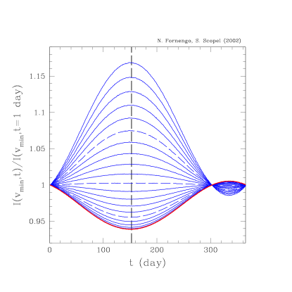
Figure 1: Time dependence of ${\cal I}(v_{\rm min})$ for an isotropic isothermal sphere. The different curves refer to values of $v_{\rm min}$ ranging from 0 (lower) to 400 (upper) Km s^-1, in steps of 20 Km s^-1 (the dashed curves correspond to $v_{\rm min}=100$, 200 and 300 Km s^-1). The vertical dashed line denotes $t=152$ days.

In the case of the isothermal sphere model the DF is given by a truncated isotropic Maxwellian which depends only on $v\equiv|\vec{v}|$:

$$f(v)=N\exp\left(-\frac{v^{2}}{2\sigma^{2}}\right)\left|\phantom{\frac{1}{2}}\right._{v\leq v_{\rm esc}},$$ (7)

where $\sigma$ is the WIMP r.m.s. velocity, given by: $\sigma^{2}=3v_{0}^{2}/2$. It is clear that, through the change of reference frame of Eq. (6), ${\cal I}(v_{\rm min})$ depends on time only through $v_{E}$. Since the relative change of $v_{E}$ during the year is of the order of a few per cent, we can approximate ${\cal I}(v_{\rm min})$ with its first–order expansion in the small parameter $\epsilon\equiv\delta v_{E}/v_{E}$, around its mean value ${\cal I}_{0}(v_{\rm min})$: ${\cal I}(v_{\rm min})-{\cal I}_{0}(v_{\rm min})\propto\cos[\omega(t-t_{0})]$. The well known result is then obtained that the WIMP rate has a sinusoidal time dependence with the same phase ($t_{0}\simeq$ June 2^nd) as $v_{E}$, for all values of $v_{\rm min}$. This is shown in Fig.1, where ${\cal I}(v_{\rm min})$ is plotted as a function of time for various values of $v_{\rm min}$.

IV Anisotropic models

The simplest generalization of the isothermal sphere model is given by a triaxial system described by a multivariate gaussian:

$$f(\vec{v})=N\exp\left(-\frac{v_{x}^{2}}{2\sigma_{x}^{2}}-\frac{v_{y}^{2}}{2\sigma_{y}^{2}}-\frac{v_{z}^{2}}{2\sigma_{z}^{2}}\right)\left|\phantom{\frac{1}{2}}\right._{v\leq v_{\rm esc}},$$ (8)

where $N$ is the normalization constant. For $v_{\rm esc}\rightarrow\infty$, then $N=[(2\pi\sigma_{x}^{2})(2\pi\sigma_{y}^{2})(2\pi\sigma_{z}^{2})]^{-1/2}$. The usual isothermal sphere is the spherical limit of Eq.(8), obtained with: $\sigma_{x}=\sigma_{y}=\sigma_{z}\equiv\sigma$. In order to discuss the effect of anisotropy at fixed WIMP mean kinetic energy, we will fix $\sigma^{2}=\sigma_{x}^{2}+\sigma_{y}^{2}+\sigma_{z}^{2}$ as in the isothermal case ($\sigma^{2}=3v_{0}^{2}/2$) and discuss our results in terms of the two independent parameters: $\lambda_{12}\equiv\sigma_{x}/\sigma_{y}$ and $\lambda_{32}\equiv\sigma_{z}/\sigma_{y}$.

At variance with the isothermal sphere, now ${\cal I}(v_{\rm min})$ depends in general on all the three components of $\vec{v}_{E}$, and not simply on $v_{E}$. We can write:

$$f_{\rm ES}(\vec{w})=N\exp\left[-(\vec{r}+\vec{\eta})^{2}\right],$$ (9)

where we have defined the reduced (dimensionless) variables: $r_{i}=w_{i}/(\sqrt{2}\sigma_{i})$ and $\eta_{i}=v^{E}_{i}/(\sqrt{2}\sigma_{i})=\eta^{0}_{i}+\delta\eta_{i}\cos[\omega(t-t_{i})]$ ($i=x,y,z$). In the isotropic case (isothermal sphere) one has $\eta^{0}_{x,z}\ll 1$, $\eta^{0}_{y}\sim 1$ and $\delta\eta_{i}\ll 1$. The presence of the order–one parameter $\eta^{0}_{y}$ and of the small oscillation amplitudes $\delta\eta_{i}$ allows the Taylor–expansion of ${\cal I}(v_{\rm min})$ in terms of $\epsilon_{i}\equiv\delta\eta_{i}/\eta^{0}_{y}$ parameters. A straightforward calculation shows that the conclusions of the previous Section are recovered.

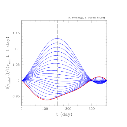
Figure 2: The same as in Fig. 1, for an anisotropic model with $\lambda_{12}\equiv\sigma_{x}/\sigma_{y}=0.2$ and $\lambda_{32}\equiv\sigma_{z}/\sigma_{y}=0.8$.

On the contrary, allowing anisotropies such that $\lambda_{12}<1$ and/or $\lambda_{32}<1$, the values of the parameters $\eta_{x,z}$ and $\delta\eta_{x,z}$ are enhanced, and the time–dependence of $v^{E}_{x}$ and $v^{E}_{z}$ in ${\cal I}(v_{\rm min})$ may become important. An example of this situation is shown in Fig. 2, where, the time evolution of ${\cal I}(v_{\rm min})$ is plotted for $\lambda_{12}=0.2$ and $\lambda_{12}=0.8$ (i.e.: $(\sigma_{x},\sigma_{y},\sigma_{z})=(42,208,166)$ Km s^-1.) This choice of $\lambda_{12}$, $\lambda_{32}$, which refers to a tangential anisotropy, corresponds to triaxial models discussed, for instance, in Refs. carollo ; galaxy . A distortion of the curves of Fig. 2, as compared to the familiar sinusoidal time–dependence, appears: this effect may be explained by the fact that now $\delta\eta_{x}\sim 1$, a Taylor–expansion of the type used in the isothermal sphere case breaks down and a full numerical calculation of the integral of Eq.(4) is required. The final result is not sinusoidal. This peculiar behaviour is more pronounced at low values of $v_{\rm min}$ (i.e. low recoil energies) namely for $v_{\rm min}\mathrel{\mathop{\kern 0.0pt\hbox to0.0pt{\raise 0.86108pt\hbox{$<$}\hss}}\lower 3.87495pt\hbox{\kern-1.90002pt$\sim$}}$ 80 Km s^-1, for which the distortion is strong and the maxima (in absolute value) of the rate are shifted as compared to the standard case krauss . For larger values of $v_{\rm min}$ the distortion is less pronounced, and it dies away when $v_{\rm min}\mathrel{\mathop{\kern 0.0pt\hbox to0.0pt{\raise 0.86108pt\hbox{$>$}\hss}}\lower 3.87495pt\hbox{\kern-1.90002pt$\sim$}}230$ Km s^-1. This may be explained by the fact that, as $v_{\rm min}$ grows, the integral of Eq.(4) becomes less sensitive to the parameter $\eta_{x}$ since it gets increasingly dominated by WIMPs with velocities along the $y$ axis, which is the one along which the boost due to the galactic rotation is directed. We notice that for values of $v_{\rm min}$ around ($100-200$) Km s^-1 a distortion is present, but the amplitude of the modulation is suppressed and therefore difficult to detect.

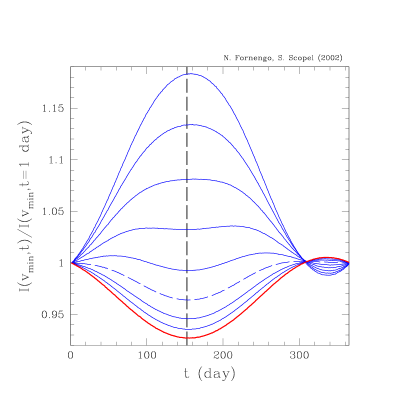
Figure 3: The same as in Fig. 1, for an anisotropic model with $\lambda_{12}\equiv\sigma_{x}/\sigma_{y}=10$ and $\lambda_{32}\equiv\sigma_{z}/\sigma_{y}=3$. The curves refer to: $v_{\rm min}=0$ (lower), 180, 190, 200 (dashed), 210, 220, 230, 240, 250 (upper) Km s^-1.

As a second example, in Fig.3 we plot ${\cal I}(v_{\rm min})$ as a function of time for the case $\lambda_{12}=10$, $\lambda_{32}=3$ (i.e.: $(\sigma_{x},\sigma_{y},\sigma_{z})=(257,26,77)$ Km s^-1. This situation is representative of a radial anisotropy. In this case, we have further enhanced the contribution of $\delta\eta_{y}$ over $\delta\eta_{x,z}$, so that one should expect to draw the same conclusions as in the isothermal sphere case, with the usual sinusoidal time–dependence of the rate and a phase close to $t_{y}\sim t_{0}$. This is indeed the case, except for a narrow interval of values of $v_{\rm min}$ around $v_{\rm min}\simeq$ 210 Km s^-1. In this range, ${\cal I}(v_{\rm min})$ develops two maxima because, for that particular choice of $v_{\rm min}$, there is an exact cancellation in the first term of the expansion in $\epsilon_{y}=\delta\eta_{y}/\eta^{0}_{y}$, so that the term ${\cal O}(\epsilon_{y}^{2})$ proportional to $\cos^{2}[\omega(t-t_{y})]$ sets in. This particular cancellation of the first term in the Taylor expansion of ${\cal I}(v_{\rm min})$ happens also for the isothermal–sphere model, but in that case the size of the quadratic term is strongly suppressed because $\epsilon_{y}$ is much smaller. In a WIMP direct detection experiment this effect would show up in a very peculiar way: a halving of the modulation period of the rate in a narrow range of recoil energies. Note, however, that in order to have some realistic chance to detect this effect, it should show up in one of the experimental energy bins just above threshold, where the highest signal/background ratio is usually attained.

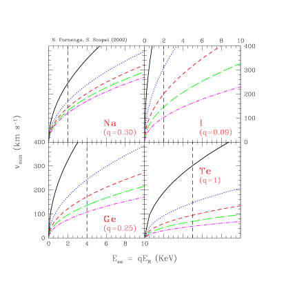
Figure 4: Values of $v_{\rm min}$ as a function of the quenched nuclear recoil energies $E_{ee}=qE_{R}$, for: NaI scintillators damalast , Ge ionization detectors direct and Te bolometers direct . For each panel, the different curves refer to WIMP masses of: 20 GeV (solid), 50 GeV (dotted), 100 GeV (dashed), 200 GeV (long–dashed) and 1 TeV (dot–dashed). The dashed vertical lines denote the current energy thresholds.

In order to establish a link between our discussion and WIMP direct detection experiments direct , in Fig. 4 we plot $v_{\rm min}$ as a function of the quenched nuclear recoil energy $E_{ee}\equiv qE_{R}$ ($q$ is the quenching factor) for the target nuclei: Na, I, Ge, Te and for different WIMP masses. The vertical dashed lines show current energy thresholds achieved by each type of detector. Fig. 4 shows that values of $v_{\rm min}\mathrel{\mathop{\kern 0.0pt\hbox to0.0pt{\raise 0.86108pt\hbox{$<$}\hss}}\lower 3.87495pt\hbox{\kern-1.90002pt$\sim$}}$ 80 Km s^-1, i.e. sufficiently low to observe a sizeable distortion effect as the one discussed for tangential anisotropy, correspond to WIMP recoil energies below the threshold of present direct detection experiments, and that the effect would be more easily detected at higher WIMP masses. However, a foreseeable lowering of the threshold, down to 0.5–1 KeV, could be enough to observe the distortion. On the other hand, for radial anisotropy, we can conclude that the recoil energy corresponding to a halving of the modulation period can actually coincide to the experimental thresholds within the reach of present–day detectors for 20 GeV $\mathrel{\mathop{\kern 0.0pt\hbox to0.0pt{\raise 0.86108pt\hbox{$<$}\hss}}\lower 3.87495pt\hbox{\kern-1.90002pt$\sim$}}m_{W}\mathrel{\mathop{\kern 0.0pt\hbox to0.0pt{\raise 0.86108pt\hbox{$<$}\hss}}\lower 3.87495pt\hbox{\kern-1.90002pt$\sim$}}$ 100 GeV, depending on the particular target nucleus. In this respect, we note that the properties of the annual modulation effect observed by the DAMA/NaI experiment damalast (a one–year–period sinusoidal behaviour in the 2–6 KeV energy bins damalast ; galaxy ) implies that the DAMA/NaI experiment is already able to set constraint on strong radial anisotropies.

V Conclusions

In the present Letter we have shown that the main features of the annual modulation of the signal of WIMP direct searches, i.e. the sinusoidal dependence of the rate with time, the position of its maxima and minima during the year and even the period, may be affected by relaxing the isothermal sphere hypothesis in the description of the WIMP velocity phase space. We have considered a multivariate gaussian and found that different situations may occur, depending on the pattern of anisotropy: tangential anisotropies induce a departure at low energies from the usual sinusoidal time–dependence, along with a shift in the position of the maximum of the signal during the year, while radial anisotropies may produce a halving of the modulation period in a particular energy bin. The former effect turns out to be relevant at low recoil energies, actually below the threshold of present–day experiments, while the latter should be already within the reach of current detectors. In particular, the properties of the annual modulation effect observed by the DAMA/NaI experiment damalast may already indicate that strong radial anisotropies are excluded.

The effects discussed in this Letter may be used in the future to provide a direct way of measuring (or setting limits on) the degree of anisotropy of the galactic halo.

References

- (1) For a summary, see, for instance: A. Morales, Nucl. Phys. Proc. Suppl. 110, 39 (2002) and references quoted therein.
- (2) A.K. Drukier, K. Freese, and D.N. Spergel, Phys. Rev. D 33, 3495 (1986); K. Freese, J. A. Frieman and A. Gould, Phys. Rev. D 37, 3388 (1988).
- (3) R. Bernabei et al. (DAMA/NaI Collaboration), Phys. Lett. B424, 195 (1998); B450, 448 (1999); B480, 23 (2000); B509, 197 (2001); Eur. Phys. J. C18, 283 (2000); C23, 61 (2002).
- (4) J.D. Lewin and P.F. Smith, Astropart. Phys. 6, 87 (1996); K.R. Lang, Astrophysical formulae, (Springer–Verlag, New York, NY, 1999).
- (5) P. Belli, R. Cerulli, N. Fornengo and S. Scopel, Phys. Rev. D 66, 043503 (2002).
- (6) N. W. Evans, C. M. Carollo and P. T. de Zeeuw, Mon. Not. Roy. Astron. Soc. 318, 1131 (2000).
- (7) A shift of the phase in triaxial halo models has also been shown in: C. J. Copi and L. M. Krauss, astro-ph/0208010.