Low-scale supersymmetry breaking: effective description, electroweak breaking and phenomenology

We consider supersymmetric scenarios in which the scale of SUSY breaking is low, $\sqrt{F}={\cal O}(\rm TeV)$. Instead of studying specific models of this type, e.g. those with extra dimensions and low fundamental scale, we follow a model-independent approach based on a general effective Lagrangian, in which the MSSM supermultiplets are effectively coupled to a singlet associated to SUSY breaking. Our goal is to analyse the interplay bewteen SUSY breaking and electroweak breaking, generalizing earlier results. The conventional MSSM picture can be substantially modified, mainly because the Higgs potential contains additional effective quartic terms and resembles that of two-Higgs-doublet models, with an additional singlet. Novel opportunities to achieve electroweak breaking arise, and the electroweak scale may be obtained in a less fine-tuned way. Also the Higgs spectrum can be strikingly changed, and the lightest state can be much heavier than in usual supersymmetric scenarios. Other effects appear in the chargino and neutralino sectors, which contain the goldstino. Finally, we discuss the role of electroweak breaking in processes in which two goldstinos could be emitted, such as fermion-antifermion annihilation and the invisible decay of a $Z$ boson or of neutral Higgs bosons.

January 2003

DFPD-02/TH/34

IFT-UAM/CSIC-02-60

IEM-FT-229/02

IPPP/02/84

DCPT/02/168

hep-ph/0301121

1 Introduction

The Minimal Supersymmetric Standard Model (MSSM) [1] has been for many years the paradigm of phenomenologically viable supersymmetric (SUSY) theories. In the MSSM the observable matter content is minimal and the breaking of SUSY (SUSY) takes place in another sector of the fundamental theory and is then transmitted to the observable sector through some mediation mechanism. As a result, one obtains a low-energy supersymmetric theory in which the MSSM multiplets are effectively coupled to the goldstino multiplet through non-renormalizable interactions, i.e. the effective Kähler potential and gauge kinetic function are generically non-minimal. Well known examples of mediation mechanisms are supergravity mediation and gauge mediation, where such effective interactions arise at the tree-level and at the loop-level respectively.

In the usual MSSM, once SUSY is broken, the effective theory is approximated by a renormalizable one, in which the SUSYsector has been decoupled, leaving as footprint a set of soft breaking terms that arise from the above effective interactions. In obtaining these soft terms the superfields responsible for SUSYplay an external role, through the expectation values of their auxiliary fields. The approximation that the soft terms encode all the effects of SUSYin the observable sector is a good one when the scale of SUSYmediation, $M$, is very large. However, in scenarios where $M$ is low (not far from the TeV scale) this picture might be not accurate enough, and the ‘hidden sector’ might be not so hidden. This already happens to some extent in gauge-mediated scenarios (see e.g. [2]), where $M\sim{\cal O}(10-10^{3})$ TeV, and also, more characteristically, in scenarios of extra dimensions (more or less string-motivated) in which the fundamental scale is quite low, typically ${\cal O}$(TeV) (see e.g. [3]). More generally, deviations from the conventional MSSM picture appear whenever the low-energy supersymmetric effective theory is obtained by integrating out physics at energy scales not far from the TeV scale. Let us briefly summarize how this comes about.

In specific models, spontaneous SUSYtakes place in a sector where the auxiliary components of a set of fields get non-vanishing vacuum expectation values (VEVs). In the simplest cases this sector can be parametrized by a single chiral superfield $T$. Then, the effective interactions between $T$ and the MSSM superfields produce at the same time: (i) SUSY breaking effects among the MSSM multiplets, as a consequence of the non-vanishing $\langle F^{T}\rangle$; (ii) specific interactions between the MSSM multiplets and the physical degrees of freedom in the $T$ multiplet, i.e. the goldstino and its scalar partners (see e.g. [4]). The form and size of these effects depend crucially on the relation between the mediation scale ($M$), the SUSY breaking scale ($\sqrt{F}$) and the electroweak scale ($M_{W}$), taking into account that the size of induced SUSYmasses, $\tilde{m}\sim F/M$, should be ${\cal O}$(TeV). In the case of a strong hierarchy $M\gg\sqrt{F}\gg M_{W}$, type (i) effects reduce to the so called ‘soft breaking terms’ [5] and type (ii) effects are negligible. This limit corresponds to the conventional MSSM. However, in the opposite case of mild (or no) hierarchy, i.e. when $M$ and $\sqrt{F}$ are in the TeV range, novel type (i) effects emerge, such as the so-called ‘non-standard soft terms’ and ‘hard breaking terms’ [6, 7]. These include, in particular, ${\cal O}(F^{2}/M^{4})$ contributions to quartic Higgs couplings, whose phenomenological impact was recently emphasized [7]. Moreover, type (ii) effects are no longer negligible and have important phenomenological consequences. For instance, goldstinos (or, equivalently [8, 9], light gravitinos) can appear in the decays of MSSM superparticles already for moderate values of $\sqrt{F}$ [10]. For sufficiently low values of $\sqrt{F}$, goldstinos can also be directly produced in high energy collisions at non-negligible rates, either in association with MSSM superparticles [11, 12, 13] or even without them [14, 15]. The scalar partners of the goldstino (sgoldstinos) can be produced as well [16, 12, 17]. Moreover, goldstinos and sgoldstinos can contribute to $(g-2)_{\mu}$ [18] and to several flavour changing or flavour conserving transitions [19, 20], and can also play a role in astrophysics and cosmology (see e.g. [21]).

The main purpose of this paper is to further explore scenarios with low SUSY breaking scale and, in particular, to analyse the interplay between SUSY breaking and electroweak breaking and to examine the Higgs sector. Since we work at the effective theory level, the field content is very economical: the only addition to the supersymmetrized Standard Model is a singlet field $T$ (responsible for SUSY), coupled non-minimally to the MSSM superfields. In section 2 we recall some general aspects of the effective description of SUSY breaking and make more explicit some of the arguments presented above. After recovering standard formulae for the MSSM mass parameters, we mention some effects expected in non-hierarchical scenarios. In section 3 we focus on the Higgs sector, analyse the pattern of electroweak symmetry breaking showing that new options are possible, and discuss the general effective interactions between the Higgs superfields and the $T$ superfield. In particular, we study how SUSY breaking effects can transform the conventional MSSM Higgs sector into a less constrained one, closer to that of generic two-Higgs-doublet models. In section 4 we make a convenient choice of field coordinates and give further details on the Higgs potential and the neutralino/chargino sectors. In section 5 we give, for illustrative purposes, two simple examples of models with low SUSYscale that have a small number of parameters. In section 6 we discuss the effective interactions involving two goldstinos and SM particles, and study how electroweak breaking affects such couplings. Finally, we summarize our results in section 7. In Appendix A we discuss the minimization of symmetric two-Higgs-doublet potentials.

2 Effective supersymmetry breaking

Throughout this paper we will describe SUSY breaking effects using an effective Lagrangian description, without relying on a specific microscopic dynamics, in an approach analogous to [4]. More specifically we will assume that, after integrating out some fundamental degrees of freedom, we are left with an effective globally supersymmetric four-dimensional theory whose degrees of freedom are the MSSM ones and a singlet chiral superfield associated with SUSY. Before discussing this, however, it is useful to recall some general properties of SUSY effective Lagrangians.

2.1 General effective Lagrangian

Let us consider a general $N=1$ globally supersymmetric theory in four dimensions, with gauge group $G$, vector superfields $V=V^{a}{\bf t}_{a}$ and chiral superfields $\phi^{i}$ (see e.g. [22]). The effective Lagrangian for such a theory has the general form

$${\cal L}=\int\!\!d^{4}\theta\left[K(\bar{\phi},e^{2V}\phi)+2\xi_{a}V^{a}\right]+\left[\int\!\!d^{2}\theta\,W(\phi)+{\rm h.c.}\right]+{1\over 4}\left[\int\!\!d^{2}\theta f_{ab}(\phi){\cal W}^{a}{\cal W}^{b}+{\rm h.c.}\right].$$ (2.1)

where $K(\bar{\phi},\phi)$, $W(\phi)$ and $f_{ab}(\phi)$ are the effective Kähler potential, superpotential and gauge kinetic functions, respectively, and higher derivative terms are neglected. The Fayet-Iliopoulos parameters $\xi_{a}$ can be non-vanishing for the abelian factors of $G$ and are shown here only for completeness (we will assume that the $\xi_{Y}$ vanishes). The effective Lagrangian for the component fields can be obtained by a standard procedure [22]. In particular, the scalar potential has the general expression

$$V=V_{F}+V_{D}=W_{i}K^{i\bar{\jmath}}\bar{W}_{\bar{\jmath}}\ +\ {1\over 2}\left[K_{i}({\bf t}_{a}\phi)^{i}+\xi_{a}\right]f_{R}^{ab}\left[K_{j}({\bf t}_{b}\phi)^{j}+\xi_{b}\right]\,.$$ (2.2)

Subscripts denote derivatives ($W_{i}\equiv\partial W/\partial\phi^{i}$, $\bar{W}_{\bar{\jmath}}\equiv\partial{\bar{W}}/\partial\bar{\phi}^{\bar{\jmath}}\equiv(\partial W/\partial\phi^{j})^{*}$, $K_{i}\equiv\partial K/\partial\phi^{i}$,…), $K^{i\bar{\jmath}}$ is the inverse of the Kähler metric $K_{\bar{\imath}j}\equiv\partial^{2}K/\partial\bar{\phi}^{\bar{\imath}}\partial\phi^{j}$ and $f_{R}^{ab}$ is the inverse of the metric $(f_{R})_{ab}\equiv{\rm Re}f_{ab}$ of the vector sector (i.e. $K^{i\bar{\jmath}}K_{\bar{\jmath}\ell}=\delta^{i}_{\ell}$ and $f_{R}^{ab}(f_{R})_{bc}=\delta^{a}_{c}$). The order parameter for supersymmetry breaking, which will be non-zero by assumption, is

$$F^{2}\equiv\langle V\rangle=\langle V_{F}+V_{D}\rangle=\langle{\bar{F}}^{\bar{\imath}}K_{\bar{\imath}j}F^{j}+{1\over 2}D^{a}(f_{R})_{ab}D^{b}\rangle\,,$$ (2.3)

where the VEVs of the auxiliary fields are

$$\langle F^{i}\rangle=-\langle K^{i\bar{\jmath}}\bar{W}_{\bar{\jmath}}\rangle\;\;,\;\;\langle D^{a}\rangle=-\langle f_{R}^{ab}\left[K_{j}({\bf t}_{b}\phi)^{j}+\xi_{b}\right]\rangle\ .$$ (2.4)

We also recall that fermion mass terms have the form $-{1\over 2}(\lambda^{a},\psi^{i}){\cal M}(\lambda^{b},\psi^{j})^{T}+{\rm h.c.}$, where the matrix ${\cal M}$ is given by

$${\cal M}=\left(\begin{array}[]{cc}-\displaystyle{1\over 2}\langle(f_{ab})_{\ell}F^{\ell}\rangle&\sqrt{2}\langle K_{\bar{\ell}j}(\overline{{\bf t}_{a}\phi})^{\bar{\ell}}+\displaystyle{1\over 4}(f_{ac})_{j}D^{c}\rangle\\ &\\ \sqrt{2}\langle K_{\bar{\ell}i}(\overline{{\bf t}_{b}\phi})^{\bar{\ell}}+\displaystyle{1\over 4}(f_{bc})_{i}D^{c}\rangle&\langle W_{ij}+{\bar{F}}^{\bar{\ell}}K_{\bar{\ell}ij}\rangle\end{array}\right)\ .$$ (2.5)

In particular, by using the extremum conditions of the scalar potential and gauge invariance, it is easy to check that the mass matrix ${\cal M}$ has an eigenvector $({1\over\sqrt{2}}\langle D^{b}\rangle,\langle F^{j}\rangle)^{T}$ with zero eigenvalue, which corresponds to the goldstino state. This eigenvector specifies the components of goldstino field $\tilde{G}$ contained in the original fields $\psi^{i}$ and $\lambda^{a}$, i.e. we have

$$\psi^{i}={\langle F^{i}\rangle\over F}\tilde{G}+\ldots\;\;,\;\;\lambda^{a}={\langle D^{a}\rangle\over\sqrt{2}F}\tilde{G}+\ldots\;\;,$$ (2.6)

where the ellipses stand for other mass eigenstates. We also recall that, in the framework of local SUSY, the goldstino degrees of freedom become the longitudinal components of the gravitino, which obtains a mass $m_{3/2}=F/(\sqrt{3}M_{P})$, where $M_{P}$ is the Planck scale. When $\sqrt{F}$ is close to the electroweak scale, $m_{3/2}$ is much smaller than typical experimental energies, which implies that the dominant gravitino components are precisely the goldstino ones [8, 9].

2.2 High and low supersymmetry breaking scales

In order to make contact with the usual MSSM framework, let us assume that the effective SUSY theory has gauge group $SU(3)\times SU(2)\times U(1)_{Y}$ and chiral superfields $\phi^{i}=(\phi^{\alpha},T)$, where $\phi^{\alpha}$ are the MSSM chiral superfields (containing Higgses, leptons and quarks) and $T$ is a singlet superfield whose auxiliary field VEV $\langle F^{T}\rangle$ breaks SUSY. For small fluctuations of the fields $\phi^{\alpha}$, the expansions of $K$, $W$ and $f_{ab}$ read

$$K = k(\bar{T},T)+c_{\bar{\alpha}\beta}(\bar{T},T)\bar{\phi}^{\bar{\alpha}}\phi^{\beta}+{1\over 2}\left[d_{\alpha\beta}(\bar{T},T)\phi^{\alpha}\phi^{\beta}+{\rm h.c.}\right]+\ldots$$ (2.7)

$$W = w(T)+{1\over 2}\mu_{\alpha\beta}(T)\phi^{\alpha}\phi^{\beta}+{1\over 3!}h_{\alpha\beta\gamma}(T)\phi^{\alpha}\phi^{\beta}\phi^{\gamma}+\ldots$$ (2.8)

$$f_{ab} = f_{a}(T)\delta_{ab}+\ldots$$ (2.9)

In the (zero-th order) vacuum defined by $\langle\phi^{\alpha}\rangle_{0}=0$, we have $F^{2}\simeq\langle V\rangle_{0}$ $=\langle|F^{T}|^{2}k_{\bar{T}T}\rangle_{0}=\langle|w_{T}|^{2}/k_{\bar{T}T}\rangle_{0}$, which by assumption is non-zero. The functions $c_{\bar{\alpha}\beta},d_{\alpha\beta},h_{\alpha\beta\gamma},f_{a}$ are assumed to depend on $T$ through the ratio $T/M$, where $M$ is some (not yet determined) scale. Then the induced SUSY-breaking mass splittings within the $\phi^{\alpha}$ and $V^{a}$ multiplets are characterized by a scale $\tilde{m}\sim F/M$. We also make the standard assumption that $\mu_{\alpha\beta}$, if non-vanishing, has size ${\cal O}(\tilde{m})$ rather than ${\cal O}(M)$, i.e. $\mu_{\alpha\beta}(T)\sim(F/M){\tilde{\mu}}_{\alpha\beta}(T/M)$.

If we fix $\tilde{m}$ to be $\cal{O}({\rm TeV})$, there is still much freedom in choosing $M$ and $F$. Standard scenarios are characterized by a strong hierarchy $M\gg\sqrt{F}\gg\tilde{m}$. In this limit the physical components of the $T$ multiplet (i.e. the goldstino and its scalar partners, the ‘sgoldstinos’) are almost decoupled from the other fields, and the effective theory for the $\phi^{\alpha}$ and $V^{a}$ multiplets is well approximated by a renormalizable one. The latter is characterized by gauge couplings $g_{a}^{2}=1/\langle{\rm Re}f_{a}\rangle_{0}$, an effective superpotential $\hat{W}$ and a set of soft SUSY breaking terms, whose mass parameters are ${\cal O}(\tilde{m})$. This is the usual MSSM scenario [1]. The MSSM parameters can be computed in terms of the functions appearing in $K$, $W$ and $f_{ab}$ above. Let us consider for simplicity the case of diagonal matter metric, i.e. $c_{\bar{\alpha}\beta}=c_{\alpha}\delta_{\bar{\alpha}\beta}$, and rescale the fields in order to have canonical normalization: $\langle\sqrt{c_{\alpha}}\rangle_{0}\phi^{\alpha}\rightarrow\phi^{\alpha}$, $\langle\sqrt{{\rm Re}f_{a}}\rangle_{0}V^{a}\rightarrow V^{a}$. The effective superpotential of the renormalizable theory is

$$\hat{W}={1\over 2}\hat{\mu}_{\alpha\beta}\phi^{\alpha}\phi^{\beta}+{1\over 3!}\hat{h}_{\alpha\beta\gamma}\phi^{\alpha}\phi^{\beta}\phi^{\gamma}\ ,$$ (2.10)

where

$$\hat{\mu}_{\alpha\beta} = \left\langle\frac{\mu_{\alpha\beta}+\bar{F}^{\bar{T}}\partial_{\bar{T}}d_{\alpha\beta}}{(c_{\alpha}c_{\beta})^{1/2}}\right\rangle_{0}\ ,$$ (2.11)

$$\hat{h}_{\alpha\beta\gamma} = \left\langle\frac{h_{\alpha\beta\gamma}}{(c_{\alpha}c_{\beta}c_{\gamma})^{1/2}}\right\rangle_{0}\ .$$ (2.12)

Soft breaking terms are described by

$${\cal L}_{\rm soft}=-\tilde{m}_{\alpha}^{2}|\phi^{\alpha}|^{2}-\left[{1\over 2}(\hat{\mu}_{\alpha\beta}B_{\alpha\beta})\phi^{\alpha}\phi^{\beta}+{1\over 3!}(\hat{h}_{\alpha\beta\gamma}A_{\alpha\beta\gamma})\phi^{\alpha}\phi^{\beta}\phi^{\gamma}+{1\over 2}M_{a}\lambda^{a}\lambda^{a}+{\rm h.c.}\right],$$ (2.13)

where

$$\tilde{m}_{\alpha}^{2} = \left\langle-|F^{T}|^{2}\partial_{T}\partial_{\bar{T}}\log c_{\alpha}\right\rangle_{0}\ ,$$ (2.14)

$$B_{\alpha\beta} = \left\langle-F^{T}\partial_{T}\log\left(\frac{\mu_{\alpha\beta}+\bar{F}^{\bar{T}}\partial_{\bar{T}}d_{\alpha\beta}}{c_{\alpha}c_{\beta}}\right)\right\rangle_{0}\ ,$$ (2.15)

$$A_{\alpha\beta\gamma} = \left\langle-F^{T}\partial_{T}\log\left(\frac{h_{\alpha\beta\gamma}}{c_{\alpha}c_{\beta}c_{\gamma}}\right)\right\rangle_{0}\ ,$$ (2.16)

$$M_{a} = \left\langle-F^{T}\partial_{T}\log({\rm Re}f_{a})\right\rangle_{0}\ .$$ (2.17)

The above results agree with [4] and are compatible with a specific limit ($M_{P}\rightarrow\infty$, $m_{3/2}\rightarrow 0$ with $F=\sqrt{3}m_{3/2}M_{P}$ fixed) of supergravity results [23].

Notice that the $T$ multiplet has played an external role in the previous derivation: it has only provided the SUSY breaking VEV $\langle F^{T}\rangle$. Moreover, only the leading terms in an expansion in $F/M^{2}$ have been retained, because of the assumed hierarchy. Other terms are strongly suppressed. However, if the scales $M$ and $F$ are not much larger than the TeV scale and the ratio $F/M^{2}\sim\tilde{m}/M\sim\tilde{m}^{2}/F$ is not negligible, the standard MSSM picture is corrected by additional effects and novel features emerge. For instance, the components of MSSM multiplets ($\phi^{\alpha}$ and $V^{a}$) can have novel non-negligible interactions among themselves as well as non-negligible interactions with the physical components of $T$ (goldstino and sgoldstinos), as we have already recalled in the introduction. Moreover, since some of the $\phi^{\alpha}$ fields (i.e. the Higgses) have to obtain a VEV in order to break the gauge symmetry, in principle one should reconsider the minimization of the scalar potential taking into account both $T$ and such fields. In addition, the $F$ components of the Higgs multiplets and the $D$ components of the neutral vector multiplets could give non-negligible contributions to SUSY breaking. In this case the goldstino could have components along all neutral fermions ($\tilde{T}$, Higgsinos and gauginos). One could even conceive extreme scenarios in which the $T$ field is absent and the Higgs fields alone are effectively responsible for breaking both SUSY and the gauge symmetry (see e.g. [24, 4], where examples of this type with singular superpotentials were given). In this paper we consider scenarios in which both $T$ and the Higgs fields are present and show how unconventional features emerge.

3 The Higgs sector

We now focus on the MSSM Higgs sector, made of two $SU(2)$ doublets $(H_{1},H_{2})$. When $F/M^{2}$ is not negligible, some higher order terms in the expansions of $K$, $W$ and $f_{ab}$ not written explicitly in eqs. (2.7), (2.8) and (2.9) can become important. We will explicitly write all the ${\cal O}(H^{4})$ terms in $W$ and $K$, which will be sufficient for our purposes. As anticipated in the previous section, the coefficient functions appearing in $W$ and $K$ will depend on the field $T$ and on some mass scales. Thus we write:

$$W = w(T)+\mu(T)H_{1}\cdot H_{2}+{1\over 2M}\ell(T)\left(H_{1}\cdot H_{2}\right)^{2}+\ldots$$ (3.1)

$$K = k(\bar{T},T)+c_{1}(\bar{T},T)|H_{1}|^{2}+c_{2}(\bar{T},T)|H_{2}|^{2}+\left[d(\bar{T},T)H_{1}\cdot H_{2}+{\rm h.c.}\right]$$ (3.2)

$$+ {1\over 2M^{2}}e_{1}(\bar{T},T)|H_{1}|^{4}+{1\over 2M^{2}}e_{2}(\bar{T},T)|H_{2}|^{4}+{1\over M^{2}}e_{3}(\bar{T},T)|H_{1}|^{2}|H_{2}|^{2}$$

$$+ {1\over M^{2}}e_{4}(\bar{T},T)|H_{1}\cdot H_{2}|^{2}+\left[{1\over 2M^{2}}e_{5}(\bar{T},T)(H_{1}\cdot H_{2})^{2}\right.$$

$$+ \left.{1\over M^{2}}e_{6}(\bar{T},T)|H_{1}|^{2}H_{1}\cdot H_{2}+{1\over M^{2}}e_{7}(\bar{T},T)|H_{2}|^{2}H_{1}\cdot H_{2}+{\rm h.c.}\right]+\ldots$$

The Kähler potential $K$ is assumed to contain a single mass scale $M$. Thus the coefficient functions $c_{i}$, $d$ and $e_{i}$ in $K$ are in fact dimensionless functions of $T/M$ and $\bar{T}/M$ while $k(\bar{T},T)\sim M^{2}\tilde{k}(\bar{T}/M,T/M)$. On the other hand, $W$ should contain, besides $M$, the SUSY-breaking scale $F$ (notice that $F\sim\langle\partial_{T}W\rangle$). Although it is not possible to determine from first principles what is the precise dependence on $M$ and $F$ of the coefficient functions in $W$, a reasonable criterion is to insure that each parameter of the component Lagrangian in the $T$-$H_{1}$-$H_{2}$ sector receives contributions of the same order from $K$ and $W$. An example of this are the two contributions to the effective $\hat{\mu}$ parameter in Eq. (2.11). The plausibility of this criterion is stressed by the fact that there is a considerable freedom to move terms between $K$ and $W$ through analytical redefinitions of the superfields (see subsection 4.1 below). Consequently, we can assume

$$w(T)\sim FM\tilde{w}(T/M)\ ,\;\;\mu(T)\sim{F\over M}\tilde{\mu}(T/M)\ ,\;\;\ell(T)\sim{F\over M^{2}}\tilde{\ell}(T/M)\ ,$$ (3.3)

where $\tilde{w},\tilde{\mu},\tilde{\ell}$ are dimensionless functions of their arguments. The above dependences can be motivated by a broken $U(1)_{R}$ symmetry under which the fields $T,H_{1},H_{2}$ and the parameter $M$ have zero charge, while $F$ has $R$-charge 2 and acts as breaking parameter. Also notice that any ($M$-dependent) non-linear field redefinition of $T,H_{1},H_{2}$ obviously respects this charge assignement.

For the expansion of the gauge kinetic functions $f_{ab}$ it is enough for our purpose to keep ${\cal O}(H^{2})$ terms. Before writing this expansion, we recall that the indices in $f_{ab}$ are saturated with those of the super-field-strengths ${\cal W}^{a}{\cal W}^{b}$, see eq. (2.1). Thus the allowed irreducible representations in $f_{ab}$ are those contained in the symmetric product of two adjoints. For the $SU(2)\times U(1)$ gauge group, such representations are singlet, triplet and fiveplet:

$$f_{ab}=f^{(s)}_{ab}+f^{(t)}_{ab}+f^{(f)}_{ab}$$ (3.4)

All these parts can be present, once $f_{ab}$ is allowed to depend on $H_{1}$ and $H_{2}$. The expansion of the singlet part $f^{(s)}_{ab}$ reads

$$f^{(s)}_{ab}=\delta_{ab}\left[f_{a}(T)+{1\over M^{2}}h_{a}(T)\,H_{1}\cdot H_{2}+\ldots\right]\,.$$ (3.5)

The triplet part $f^{(t)}_{ab}$ is associated with the $SU(2)$-$U(1)_{Y}$ cross-term ${\cal W}^{A}{\cal W}^{Y}$, where $A$ is an $SU(2)$ index. Thus the non-vanishing components of $f^{(t)}_{ab}$ are $f^{(t)}_{AY}=f^{(t)}_{YA}$ and their expansion starts at ${\cal O}(H^{2})$:

$$f^{(t)}_{AY}={1\over M^{2}}\omega(T)\,(H_{1}\cdot\sigma^{A}H_{2})+\ldots$$ (3.6)

In eqs. (3.5,3.6) we have inserted appropriate powers of $M^{2}$ as before, and we can assume that $f_{a}$, $h_{a}$ and $\omega$ are dimensionless functions of $T/M$. Finally, the fiveplet part $f^{(f)}_{ab}$ has both indices in $SU(2)$. We will neglect this part since its leading term is ${\cal O}(H^{4})$.

3.1 Scalar potential and electroweak breaking

From $W$, $K$ and $f_{ab}$ one can compute the component Lagrangian, and in particular the scalar potential, which is given by the general expression in eq. (2.2). It is clear that the expanded form of $V$ will be similar to that of $K$. More precisely, $V$ has the same form as in a two-Higgs-doublet model (2HDM), with $T$-dependent coefficients, i.e.

$$V = V_{0}(\bar{T},T)+m_{1}^{2}(\bar{T},T)|H_{1}|^{2}+m_{2}^{2}(\bar{T},T)|H_{2}|^{2}+\left[m_{3}^{2}(\bar{T},T)H_{1}\cdot H_{2}+{\rm h.c.}\right]$$ (3.7)

$$+ {1\over 2}\lambda_{1}(\bar{T},T)|H_{1}|^{4}+{1\over 2}\lambda_{2}(\bar{T},T)|H_{2}|^{4}+\lambda_{3}(\bar{T},T)|H_{1}|^{2}|H_{2}|^{2}+\lambda_{4}(\bar{T},T)|H_{1}\cdot H_{2}|^{2}$$

$$+ \left[{1\over 2}\lambda_{5}(\bar{T},T)(H_{1}\cdot H_{2})^{2}+\lambda_{6}(\bar{T},T)|H_{1}|^{2}H_{1}\cdot H_{2}+\lambda_{7}(\bar{T},T)|H_{2}|^{2}H_{1}\cdot H_{2}+{\rm h.c.}\right]$$

$$+ \ldots$$

where we have truncated at ${\cal O}(H^{4})$. The parametric dependence of the coefficients in $V$ is $m_{i}^{2}\sim{\cal O}(F^{2}/M^{2})$ and $\lambda_{i}\sim{\cal O}(F^{2}/M^{4})+{\cal O}(g^{2})$. Explicit expressions for $m_{i}^{2}(\bar{T},T)$ can be deduced from the results of sect. 2.2, whilst the form of the coefficients $\lambda_{i}(\bar{T},T)$ will be discussed in detail in sect. 4.2.

In general, for a given potential, one can try to perform either an exact minimization or at least an iterative one, relying on the expansion of the potential in powers of $H_{i}/M$ and on the consistent assumption that the Higgs VEVs are smaller than $M$, possibly through some tuning. In the iterative approach, the starting point for the determination of the VEVs are the zero-th order values of $\langle H_{i}^{0}\rangle_{0}$ and $\langle T\rangle_{0}$, where $\langle H_{i}^{0}\rangle_{0}=0$ and $\langle T\rangle_{0}$ is the minimum of $V_{0}(\bar{T},T)$.

In sections 4, 5 and 6 we will discuss in more detail the scalar potential, its minimization and other phenomenological implications, both in general and through specific examples. Here we note that the form of the Higgs potential in eq. (3.7) already allows us to make some general observations on the possible patterns of electroweak breaking. Let us set $m_{i}^{2}\equiv\langle m_{i}^{2}(\bar{T},T)\rangle_{0}$ for brevity. There are two necessary conditions for electroweak breaking, which for a polynomial Higgs potential imply the existence of a non-trivial minimum.

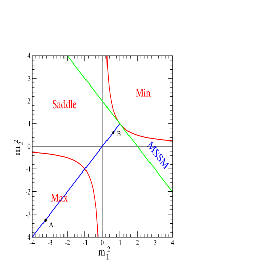
Figure 1: Schematic representation of the different possibilities for electroweak breaking in a two-Higgs-doublet model, depending on the values of $m_{1}^{2}$ and $m_{2}^{2}$ (with the axes in units of $|m_{3}^{2}|$). See text for details.

The first condition regards the origin of Higgs-field space. This is a minimum, a saddle point or a maximum, depending on the mass parameters $m_{i}^{2}$:

$$m_{1}^{2}m_{2}^{2}-|m_{3}^{2}|^{2} > 0\ ,\ m_{1}^{2}+m_{2}^{2}\ >\ 0\ .\hskip 51.21504pt[\mathrm{Minimum}]$$ (3.8)

$$m_{1}^{2}m_{2}^{2}-|m_{3}^{2}|^{2} < 0\ ,\hskip 119.50148pt[\mathrm{Saddle\ Point}]$$ (3.9)

$$m_{1}^{2}m_{2}^{2}-|m_{3}^{2}|^{2} > 0\ ,\ m_{1}^{2}+m_{2}^{2}\ <\ 0\ .\hskip 51.21504pt[\mathrm{Maximum}]$$ (3.10)

These equations define three regions in the $\{m_{1}^{2},m_{2}^{2}\}$-plane, labelled by ‘Min’, ‘Saddle’ and ‘Max’ in Fig. 1. Such regions are separated by the upper and lower branches of the hyperbola $m_{1}^{2}m_{2}^{2}-|m_{3}^{2}|^{2}=0$. Electroweak breaking can take place in the regions ‘Saddle’ or ‘Max’, while the region ‘Min’ is excluded.

The second condition for proper electroweak breaking is the absence of unbounded from below directions (UFB) along which the quartic part of the Higgs potential gets destabilized. As a matter of fact the complete Higgs potential is necessarily bounded from below since the full supersymmetric potential (2.2) is positive definite. However, this does not guarantee that the truncation of $V$ at ${\cal O}(H^{4})$, i.e. eq. (3.7), is positive as well. If it is not, this means that the positivity of the potential is ensured by higher order terms and the minima correspond to large values of $H_{i}$, which is not phenomenologically acceptable. UFB directions of this kind are normally prevented by quartic couplings. In the MSSM the latter receive only contributions from D-terms, namely $\lambda_{1,2}={1\over 4}(g^{2}+g_{Y}^{2})$, $\lambda_{3}={1\over 4}(g^{2}-g_{Y}^{2})$, $\lambda_{4}=-{1\over 2}g^{2}$, $\lambda_{5,6,7}=0$. Then the potential is indeed stabilized by the quartic terms, except along the D-flat directions $|H_{1}|=|H_{2}|$. Consequently, it is required that the quadratic part of $V$ be positive along these directions:

$$m_{1}^{2}+m_{2}^{2}-2|m_{3}^{2}|>0\ .\hskip 56.9055pt[\mathrm{Potential\ bounded\ from\ below}]$$ (3.11)

This condition applies only to the MSSM and corresponds to the region of Fig. 1 above the straight line tangent to the upper branch of the hyperbola. Since eq. (3.11) is incompatible with eq. (3.10), it follows that the MSSM conditions for electroweak breaking are given by eqs.(3.9,3.11), as is well known. In Fig. 1 the corresponding region is a subset of the region ‘Saddle’ and is labelled by ‘MSSM’: it is made of the (two) areas between the upper branch of the hyperbola and the tangent line.

However, when SUSY is broken at a moderately low scale, the $\lambda_{i}$ couplings in (3.7) can also receive sizeable ${\cal O}(F^{2}/M^{4})$ contributions, besides the ${\cal O}(g^{2})$ ones. Therefore condition (3.11) is no longer mandatory to avoid UFB directions, since the boundedness of the potential can be ensured by imposing appropriate conditions on the $\lambda_{i}$ parameters. Thus the presence of the latter parameters extends the parameter space, relaxes the constraints on the quadratic part of the potential and opens a lot of new possibilities for electroweak breaking. In particular, both alternatives (3.9, 3.10) are now possible. This means that most of the $\{m_{1}^{2},m_{2}^{2}\}$ plane can in principle be explored: the whole regions labelled by ‘Saddle’ and ‘Max’ in Fig. 1 are allowed, only the region ‘Min’ is excluded. This has several important consequences, that differ from usual MSSM results, and which we list below.

(a)

The universal case $m_{1}^{2}=m_{2}^{2}$ is now allowed, unlike in the MSSM. Actually, in the MSSM these mass parameters could be degenerate at high energy and reach non-degenerate values radiatively by RG running (falling in the region ‘MSSM’ of Fig. 1, typically with $m_{1}^{2}>0$, $m_{2}^{2}<0$). The fact that $m_{2}^{2}$ is the only scalar mass that tends to get negative in this process is considered one of the virtues of the MSSM, in the sense that $SU(2)\times U(1)$ breaking is “natural”. Now, we see that even if the universal condition holds at low-energy we can still break $SU(2)\times U(1)$. This will be illustrated in section 5 with two examples, which correspond to points A and B in Fig. 1. We will also show that $m_{1}^{2}=m_{2}^{2}$ does not necessarily imply $\langle|H_{1}|\rangle=\langle|H_{2}|\rangle$, i.e. $|\tan\beta|=1$.

(b)

Electroweak breaking generically occurs already at tree-level. Still, it is “natural” in a sense similar to the MSSM. For example, if all the scalar masses are positive and universal, $SU(2)_{L}\times U(1)_{Y}$ is the only symmetry that can be broken because (with R-parity conserved) the only off-diagonal bilinear coupling among MSSM fields is $m_{3}^{2}\,H_{1}\cdot H_{2}$, which can drive symmetry breaking in the Higgs sector if condition (3.9) is satisfied. This is just an example: we stress again that many unconventional possibilities for electroweak breaking are allowed, including those in which both $m_{1}^{2}$ and $m_{2}^{2}$ are negative and $m_{3}^{2}$ plays a minor role.

(c)

Finally, the fact that quartic couplings are very different from those of the MSSM changes dramatically the Higgs spectrum and properties (which will be tested at colliders, see e.g. [29, 30]). In particular, as illustrated by later examples, the MSSM bound on the lightest Higgs field does no longer apply. Likewise, the fact that these couplings can be larger than the MSSM ones may reduce the amount of tuning necessary to get the proper Higgs VEVs. Concerning the latter property, suppose that $F^{2}/M^{2}$ is significantly larger than the phenomenologically required value of $v^{2}$. In this case, as is well known in the MSSM, only one combination of the $m_{i}^{2}$ is allowed to be as large as ${\cal O}(F^{2}/M^{2})$, whereas two other combinations should be tuned to values ${\cal O}(\lambda_{i}v^{2})$, as a consequence of the minimization conditions. The interesting point is that the ${\cal O}(F^{2}/M^{4})$ contributions to the couplings $\lambda_{i}$ can exceed the familiar ${\cal O}(g^{2})$ contributions, so the amount of fine tuning can be somewhat alleviated.

3.2 Derivative couplings and the $\rho$-parameter

In addition to modifications in the Higgs potential, the non-renormalizable terms in the Kähler potential (3.2) generate derivative couplings. Explicitly, the generalized kinetic Lagrangian for $H_{1},H_{2},T$ reads

$${\cal L}_{kin} = |D_{\mu}H_{1}|^{2}\left[c_{1}+{e_{1}\over M^{2}}|H_{1}|^{2}+{e_{3}\over M^{2}}|H_{2}|^{2}+\left({e_{6}\over M^{2}}H_{1}\cdot H_{2}+{\mathrm{h}.c.}\right)\right]$$ (3.12)

$$+ |D_{\mu}H_{2}|^{2}\left[c_{2}+{e_{2}\over M^{2}}|H_{2}|^{2}+{e_{3}\over M^{2}}|H_{1}|^{2}+\left({e_{7}\over M^{2}}H_{1}\cdot H_{2}+{\mathrm{h}.c.}\right)\right]$$

$$+ |\partial_{\mu}T|^{2}\left[k_{T\bar{T}}+({c_{1}})_{T\bar{T}}|H_{1}|^{2}+({c_{2}})_{T\bar{T}}|H_{2}|^{2}+\left(d_{T\bar{T}}H_{1}\cdot H_{2}+{\mathrm{h}.c.}\right)\right]$$

$$+ {e_{1}\over M^{2}}|H_{1}^{\dagger}D_{\mu}H_{1}|^{2}+{e_{2}\over M^{2}}|H_{2}^{\dagger}D_{\mu}H_{2}|^{2}$$

$$+ {e_{3}\over M^{2}}\left[H_{1}^{\dagger}D_{\mu}H_{1}(D^{\mu}{H}_{2})^{\dagger}H_{2}+{\mathrm{h}.c.}\right]+{e_{4}\over M^{2}}|\partial_{\mu}(H_{1}\cdot H_{2})|^{2}$$

$$+ \left\{\left[{e_{6}\over M^{2}}(D^{\mu}{H}_{1})^{\dagger}H_{1}+{e_{7}\over M^{2}}(D^{\mu}{H}_{2})^{\dagger}H_{2}\right]\partial_{\mu}(H_{1}\cdot H_{2})+{\mathrm{h}.c.}\right\}$$

$$+ \left\{\partial_{\mu}T^{*}\left[({c_{1}})_{\bar{T}}H_{1}^{\dagger}D^{\mu}H_{1}+({c_{2}})_{\bar{T}}H_{2}^{\dagger}D^{\mu}H_{2}+d_{\bar{T}}\partial^{\mu}(H_{1}\cdot H_{2})\right]+{\mathrm{h}.c.}\right\}$$

$$+ \ldots\ ,$$

where $|X_{\mu}|^{2}\equiv X_{\mu}^{*}X^{\mu}$ and $c_{i}$, $e_{i}$, $k$, $d$ are the $T,\bar{T}$-dependent functions that appear in (3.2). Thus the Higgses and the $T$ scalars also have derivative interactions, besides the non-derivative ones described by the scalar potential. Moreover, since the derivatives are gauge-covariant, non-renormalizable interactions between scalar and vector fields appear as well.

One of the consequences of electroweak symmetry breaking [$\langle H_{i}^{0}\rangle=v_{i}/\sqrt{2}$, $\tan\beta\equiv v_{2}/v_{1}$, $v^{2}\equiv v_{1}^{2}+v_{2}^{2}$] is that ${\cal L}_{kin}$ generates mass terms for the gauge bosons. Let us normalize the Higgs fields so that $\langle c_{i}\rangle_{0}=1$, which implies $\langle c_{i}\rangle=1+{\cal O}(v^{2}/M^{2})$, and assume real parameters for simplicity. We also temporarily neglect the non-singlet parts of $f_{ab}$, so gauge couplings are defined by $\langle{\rm Re}f_{ab}^{(s)}\rangle=g_{a}^{-2}\delta_{ab}$. The gauge boson masses are:

$$M_{W}^{2} = {1\over 4}g^{2}{\hat{v}}^{2}\ ,$$ (3.13)

$$M_{Z}^{2} = {1\over 4}(g^{2}+g_{Y}^{2})\left[{\hat{v}}^{2}+{v^{4}\over 2M^{2}}\langle e_{1}c_{\beta}^{4}+e_{2}s_{\beta}^{4}-2e_{3}s^{2}_{\beta}c^{2}_{\beta}\rangle+\ldots\right]\ ,$$ (3.14)

with

$${\hat{v}}^{2} = v^{2}\left[\langle c_{1}c^{2}_{\beta}+c_{2}s^{2}_{\beta}\rangle+{v^{2}\over 2M^{2}}\langle e_{1}c_{\beta}^{4}+e_{2}s_{\beta}^{4}+2e_{3}s^{2}_{\beta}c^{2}_{\beta}+(e_{6}c_{\beta}^{2}+e_{7}s^{2}_{\beta})s_{2\beta}\rangle+\ldots\right]$$ (3.15)

$$= v^{2}\left[1+{\cal O}(v^{2}/M^{2})\right]\ .$$

We see first that there is a small deviation of the Higgs VEV $v$ from ${\hat{v}}=246$ GeV [of relative order ${\cal O}(v^{2}/M^{2})$, which we will ignore in the following], and second there is a non-zero contribution to $\Delta\rho$ (i.e. $\epsilon_{1}$ or $\alpha\Delta T$), given by

$$\Delta\rho=-{v^{2}\over 2M^{2}}\left[c_{\beta}^{4}\langle e_{1}\rangle_{0}+s_{\beta}^{4}\langle e_{2}\rangle_{0}-2s_{\beta}^{2}c_{\beta}^{2}\langle e_{3}\rangle_{0}\right]+{\cal O}(v^{4}/M^{4})\ .$$ (3.16)

This combination of parameters is constrained to be small by electroweak precision measurements [31], which could be used, for instance, to infer a lower bound on the scale $M$, for given values of $\langle e_{i}\rangle_{0}$ and $\tan\beta$, or to constrain the parameters $\langle e_{i}\rangle_{0}$, for given $M$ and $\tan\beta$. Notice that a natural suppression of $\Delta\rho$ is obtained if the Kähler potential has an approximate $SU(2)_{L}\times SU(2)_{R}$ symmetry, since the latter implies the equality $e_{1}=e_{2}=e_{3}$, and also $|\tan\beta|=1$ after electroweak breaking (see also Appendix A).

Another set of non-renormalizable interactions between scalar and vector fields originate from the gauge kinetic terms, i.e. from the field dependence of the kinetic functions $f_{ab}(T,H_{1},H_{2})$. In particular, the $T$ dependence of $f_{ab}$, which is responsible for the leading contribution to gaugino masses [eq. (2.17)] and to goldstino-gaugino-gauge boson couplings, also induces interactions of the $T$ scalar field with two gauge field strengths. The latter interactions are relevant, for instance, in the production and decays of $T$ scalars at colliders [16, 12, 17]. Similarly, the dependence of $f_{ab}$ on $H_{1}$ and $H_{2}$ could have interesting implications for the production and decays of Higgs bosons. In the latter case, the relevant part of $f_{ab}$ is probably the singlet part $f_{ab}^{(s)}$, since the non-singlet parts are more constrained or suppressed. In particular, we recall that the triplet part $f_{ab}^{(t)}$ of $f_{ab}$, eq. (3.6), produces a kinetic mixing between the $SU(2)_{L}$ and the $U(1)_{Y}$ field strengths once the Higgs fields take VEVs. This effect modifies the expressions of the gauge boson masses and couplings, and one obtains a contribution to the $\epsilon_{3}$ parameter (or $\alpha S$) proportional to $s_{\beta}c_{\beta}\langle\omega\rangle_{0}v^{2}/M^{2}$, which is therefore constrained to be small. Finally, we note that contributions to the $\epsilon_{2}$ parameter (or $\alpha U$) are automatically more suppressed, since they arise from the fiveplet part $f_{ab}^{(f)}$ of $f_{ab}$ and are ${\cal O}(s_{\beta}^{2}c_{\beta}^{2}v^{4}/M^{4})$.

4 General results in normal coordinates

4.1 Coordinate choices

Theories with different expressions for $K$, $W$ and $f_{ab}$ have the same physical content if they are related by analytic redefinitions of the chiral superfields. This well known property is already clear, for instance, in the results for the MSSM mass parameters presented in section 2: the spectrum only depends on specific combinations of the original parameters. The effective $\hat{\mu}$ parameter of eq. (2.11) is a well known example: its two ‘components’ (from $W$ and $K$) can easily be moved into one another by a redefinition of the $T$ field that involves the Higgs fields. For instance, if $K\supset|T|^{2}-\left({\beta_{\mu}\over M}\bar{T}H_{1}\cdot H_{2}+{\rm h.c.}\right)$ and $W\supset\Lambda_{S}^{2}T$, the redefinition $T=T^{\prime}+{\beta_{\mu}\over M}H_{1}\cdot H_{2}$ leads to $K\supset|T^{\prime}|^{2}-{|\beta_{\mu}|^{2}\over M^{2}}|H_{1}\cdot H_{2}|^{2}$ and $W\supset\Lambda_{S}^{2}T^{\prime}+\beta_{\mu}{\Lambda_{S}^{2}\over M}H_{1}\cdot H_{2}$. Either coordinate choice leads to the same effective $\hat{\mu}$ parameter.

Sometimes it is better to avoid such field redefinitions, in order to keep track of all the different ‘sources’ of a specific effective parameter or coupling. At other times, it is convenient to exploit such redefinitions in order to reduce the redundant set of parameters to a minimal set. For instance, one can try to remove as many terms as possible from the superpotential and reduce it to a minimal one. In our case we could first shift $T$ so that its zero-th order VEV vanish, $\langle T\rangle_{0}=0$, and then redefine the whole $W(T,H_{1},H_{2})$ to be just the new $T$ field, i.e. $W(T,H_{1},H_{2})=\Lambda_{S}^{2}T^{\prime}$, where $\Lambda_{S}^{2}\sim F$ (SUSY breaking scale). An advantage of this coordinate choice is that all the parameters in the component Lagrangian automatically have a simple dependence on $F$ and $M$, e.g. $\hat{\mu}\sim F/M$. An example with such a minimal superpotential will be described in section 5. Another possibility, orthogonal to the previous one, is to remove as many terms as possible from $K$. In general, one can set to zero all the derivatives $K_{\bar{I}J_{1}J_{2}\ldots J_{n}}$ ($n>1$) and their conjugates around a given point [32] (Kähler normal coordinates). In our case we could first shift $T$ so that $\langle T\rangle_{0}=0$ and then use normal coordinates around the origin. In the next subsections we will make this choice and present explicit results on the scalar potential and the fermionic spectrum. Of course, it is also possible to employ intermediate coordinate choices, or even to make no coordinate choice at all, with equivalent results.

4.2 The scalar potential

The form of $W$ and $K$ [see Eqs.(3.1, 3.2)] expressed in normal coordinates and expanded in the $H_{i}$ and $T$ fields reads

$$W = \Lambda_{S}^{2}\left(T+{1\over 6M^{2}}\rho_{t}T^{3}+\ldots\right)+\left(\mu+\mu^{\prime}{T\over M}+{1\over 2}\mu^{\prime\prime}{T^{2}\over M^{2}}+\ldots\right)H_{1}\cdot H_{2}$$ (4.1)

$$+ {1\over 2M}\left(\ell+\ell^{\prime}{T\over M}+\ldots\right)\left(H_{1}\cdot H_{2}\right)^{2}+\ldots$$

$$K = \left(|T|^{2}-{1\over 4}\alpha_{t}{|T|^{4}\over M^{2}}+\ldots\right)+|H_{1}|^{2}\left[1+\alpha_{1}{|T|^{2}\over M^{2}}+{1\over 2M^{3}}(\alpha^{\prime}_{1}T^{2}\bar{T}+\bar{\alpha}^{\prime}_{1}T\bar{T}^{2})+\ldots\right]$$ (4.2)

$$+ |H_{2}|^{2}\left[1+\alpha_{2}{|T|^{2}\over M^{2}}+{1\over 2M^{3}}(\alpha^{\prime}_{2}T^{2}\bar{T}+\bar{\alpha}^{\prime}_{2}T\bar{T}^{2})+\ldots\right]$$

$$+ \left[H_{1}\cdot H_{2}\left({1\over 2}\alpha_{3}{\bar{T}^{2}\over M^{2}}+{1\over 2M^{3}}\alpha_{3}^{\prime}\bar{T}^{2}T+\ldots\right)+{\rm h.c.}\right]$$

$$+ {1\over M^{2}}\left\{{1\over 2}|H_{1}|^{4}\left[e_{1}+{1\over M}(e^{\prime}_{1}T+\bar{e}^{\prime}_{1}\bar{T})+e^{\prime\prime}_{1}{|T|^{2}\over M^{2}}+\ldots\right]\right.$$

$$+ {1\over 2}|H_{2}|^{4}\left[e_{2}+{1\over M}(e^{\prime}_{2}T+\bar{e}^{\prime}_{2}\bar{T})+e^{\prime\prime}_{2}{|T|^{2}\over M^{2}}+\ldots\right]$$

$$+ |H_{1}|^{2}|H_{2}|^{2}\left[e_{3}+{1\over M}(e^{\prime}_{3}T+\bar{e}^{\prime}_{3}\bar{T})+e^{\prime\prime}_{3}{|T|^{2}\over M^{2}}+\ldots\right]$$

$$+ |H_{1}\cdot H_{2}|^{2}\left[e_{4}+{1\over M}(e^{\prime}_{4}T+\bar{e}^{\prime}_{4}\bar{T})+e^{\prime\prime}_{4}{|T|^{2}\over M^{2}}+\ldots\right]$$

$$+ \left[|H_{1}|^{2}H_{1}\cdot H_{2}\left(e^{\prime}_{6}{\bar{T}\over M}+e^{\prime\prime}_{6}{|T|^{2}\over M^{2}}+\ldots\right)+{\rm h.c.}\right]$$

$$+ \left.\left[|H_{2}|^{2}H_{1}\cdot H_{2}\left(e^{\prime}_{7}{\bar{T}\over M}+e^{\prime\prime}_{7}{|T|^{2}\over M^{2}}+\ldots\right)+{\rm h.c.}\right]\right\}+\ldots$$

It is not restrictive to take $\Lambda_{S}^{2}$ real and positive. The coefficients of real invariants in $K$ (e.g. $\alpha_{t},\alpha_{1},\alpha_{2},\ldots$) are necessarily real. For the sake of generality we allow other parameters to be complex, keeping in mind that they should be taken as real if $CP$ conservation is imposed. The terms explicitly shown above are sufficient to compute all the ${\cal O}(T^{2})$, ${\cal O}(H^{2})$, ${\cal O}(TH^{2})$, and ${\cal O}(H^{4})$ terms of the scalar potential, which in turn are sufficient to evaluate VEVs and spectrum at lowest non-trivial order in $v/M$. Also notice that, to this purpose, it is sufficient to keep the zero-th order part of $f_{ab}$, i.e. $\delta_{ab}/g_{a}^{2}$. We postpone the explicit expansion of $f_{ab}$ to the discussion of fermion masses below. It is also convenient to define the auxiliary quantity

$$\tilde{m}\equiv{\Lambda_{S}^{2}\over M}\ ,$$ (4.3)

which controls the typical magnitude of SUSY-breaking masses and appears frequently in what follows. In doing parametric estimates we will also apply eq. (3.3), i.e. we will implicitly assume $\mu,\mu^{\prime},\mu^{\prime\prime}={\cal O}(\tilde{m})$ and $\ell,\ell^{\prime}={\cal O}(\tilde{m}/M)$.

The scalar potential $V=V_{F}+V_{D}$ can be computed from the general expression (2.2) and expanded as in eq. (3.7). The latter expansion can be further specialized using the above parametrization of $W$ and $K$. We obtain:

$$V = \Lambda_{S}^{4}+\alpha_{t}\tilde{m}^{2}|T|^{2}+{1\over 2}(\rho_{t}\tilde{m}^{2}T^{2}+{\rm h.c.})+m_{1}^{2}|H_{1}|^{2}+m_{2}^{2}|H_{2}|^{2}+\left(m_{3}^{2}H_{1}\cdot H_{2}+{\rm h.c.}\right)$$ (4.4)

$$+ (a_{1}T+\bar{a}_{1}\bar{T})|H_{1}|^{2}+(a_{2}T+\bar{a}_{2}\bar{T})|H_{2}|^{2}+\left[(a_{3}T+a_{4}\bar{T})H_{1}\cdot H_{2}+{\rm h.c.}\right]$$

$$+ {1\over 2}\lambda_{1}|H_{1}|^{4}+{1\over 2}\lambda_{2}|H_{2}|^{4}+\lambda_{3}|H_{1}|^{2}|H_{2}|^{2}+\lambda_{4}|H_{1}\cdot H_{2}|^{2}$$

$$+ \left[{1\over 2}\lambda_{5}\left(H_{1}\cdot H_{2}\right)^{2}+\lambda_{6}|H_{1}|^{2}H_{1}\cdot H_{2}+\lambda_{7}|H_{2}|^{2}H_{1}\cdot H_{2}+{\rm h.c.}\right]+\ldots$$

The coefficients of the ${\cal O}(T^{2})$ terms should satisfy $\alpha_{t}>|\rho_{t}|$, for consistency with the condition $\langle T\rangle_{0}=0$. The two degrees of freedom of the complex field $T$ have masses $m_{T_{1,2}}^{2}=(\alpha_{t}\pm|\rho_{t}|)\tilde{m}^{2}$, which are ${\cal O}(\Lambda_{S}^{4}/M^{2})$.

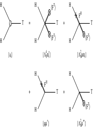
Figure 2: Diagrammatic origin of different contributions to the cubic $H^{2}T$ couplings [$a_{i}$ in Eq. (4.6)].

The coefficients of the ${\cal O}(H^{2})$ terms of $V$ are given by

$$m_{1}^{2}=|\mu|^{2}-\alpha_{1}\tilde{m}^{2}\;,\;\;\;\;m_{2}^{2}=|\mu|^{2}-\alpha_{2}\tilde{m}^{2}\;,\;\;\;\;m_{3}^{2}=\mu^{\prime}\tilde{m}\ ,$$ (4.5)

and are generically ${\cal O}(\tilde{m}^{2})={\cal O}(\Lambda_{S}^{4}/M^{2})$. The coefficients of the ${\cal O}(TH^{2})$ terms of $V$ are given by

$$a_{1}=-{1\over M}(\alpha^{\prime}_{1}\tilde{m}^{2}+\bar{\alpha}_{3}\mu\tilde{m}-\bar{\mu}\mu^{\prime})\ \;\;a_{3}={\displaystyle{1\over M}}\tilde{m}\mu^{\prime\prime}\ ,$$ ,

$$a_{2}=-{\displaystyle{1\over M}}(\alpha^{\prime}_{2}\tilde{m}^{2}+\bar{\alpha}_{3}\mu\tilde{m}-\bar{\mu}\mu^{\prime})\ \;\;a_{4}=-{\displaystyle{1\over M}}[\alpha^{\prime}_{3}\tilde{m}^{2}+(\alpha_{1}+\alpha_{2})\mu\tilde{m}]\ ,$$ , (4.6)

and are generically ${\cal O}(\tilde{m}^{2}/M)={\cal O}(\Lambda_{S}^{4}/M^{3})$. The origin of the different contributions to these cubic couplings is traced back to the diagrams in Fig. 2, which carry self-explanatory labels. Double lines represent auxiliary fields and crossed circles represent the lowest order VEV $\langle F^{T}\rangle_{0}=-\Lambda_{S}^{2}$.

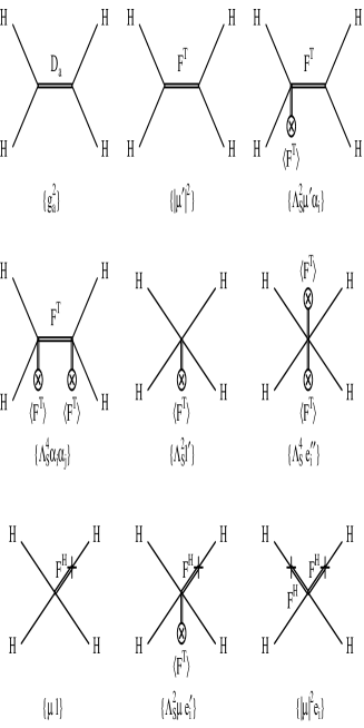
Figure 3: Diagrammatic origin of different contributions to the quartic Higgs couplings [$\lambda_{i}$ in Eqs. (4.8) and (4.9)].

Finally, the coefficients of the ${\cal O}(H^{4})$ terms of $V$ (quartic in the Higgs fields without $T$) receive two different types of contributions:

$$\lambda_{i}=\lambda_{i}^{(D)}+\lambda_{i}^{(F)}\ .$$ (4.7)

The $\lambda_{i}^{(D)}$ arise from $V_{D}$ as usual:

$$\lambda_{1}^{(D)}=\lambda_{2}^{(D)}={1\over 4}(g^{2}+g_{Y}^{2})\ ,\;\;\lambda_{3}^{(D)}={1\over 4}(g^{2}-g_{Y}^{2})\ ,\;\;\lambda_{4}^{(D)}=-{1\over 2}g^{2}\ ,$$ (4.8)

while $\lambda_{5}^{(D)}=\lambda_{6}^{(D)}=\lambda_{7}^{(D)}=0$. The $\lambda_{i}^{(F)}$ are the direct contributions from the ${\cal O}(H^{4})$ terms in $V_{F}$:

$$\lambda_{1}^{(F)} = {1\over M^{2}}\left[\tilde{m}^{2}(2\alpha_{1}^{2}-e^{\prime\prime}_{1})-2\tilde{m}(\bar{\mu}e^{\prime}_{6}+{\rm h.c.})-2|\mu|^{2}(e_{3}+e_{4})\right]\ ,$$

$$\lambda_{2}^{(F)} = {1\over M^{2}}\left[\tilde{m}^{2}(2\alpha_{2}^{2}-e^{\prime\prime}_{2})-2\tilde{m}(\bar{\mu}e^{\prime}_{7}+{\rm h.c.})-2|\mu|^{2}(e_{3}+e_{4})\right]\ ,$$

$$\lambda_{3}^{(F)} = {1\over M^{2}}\left[\tilde{m}^{2}(2\alpha_{1}\alpha_{2}-e^{\prime\prime}_{3})-\tilde{m}\left[\bar{\mu}(e^{\prime}_{6}+e^{\prime}_{7})+{\rm h.c.}\right]-|\mu|^{2}(e_{1}+e_{2}+2e_{4})\right]\ ,$$

$$\lambda_{4}^{(F)} = -{1\over M^{2}}\left[\tilde{m}^{2}e^{\prime\prime}_{4}+\tilde{m}\left[(e^{\prime}_{6}+e^{\prime}_{7})\bar{\mu}+{\rm h.c.}\right]+|\mu|^{2}(e_{1}+e_{2}+2e_{3})-|\mu^{\prime}|^{2}\right]\ ,$$

$$\lambda_{5}^{(F)} = {\ell^{\prime}\tilde{m}\over M}\ ,$$

$$\lambda_{6}^{(F)} = -{1\over M^{2}}\left[\tilde{m}^{2}e^{\prime\prime}_{6}+\tilde{m}\left[\mu(e^{\prime}_{1}+e^{\prime}_{3}+e^{\prime}_{4})+\mu^{\prime}\alpha_{1}\right]\right]+{\ell\bar{\mu}\over M}\ ,$$

$$\lambda_{7}^{(F)} = -{1\over M^{2}}\left[\tilde{m}^{2}e^{\prime\prime}_{7}+\tilde{m}\left[\mu(e^{\prime}_{2}+e^{\prime}_{3}+e^{\prime}_{4})+\mu^{\prime}\alpha_{2}\right]\right]+{\ell\bar{\mu}\over M}\ .$$ (4.9)

Figure 3 shows the diagrammatic origin of these terms, again with labels as appropriate to identify different types of contributions. The parameters $\lambda_{i}^{(F)}$ are generically ${\cal O}(\tilde{m}^{2}/M^{2})={\cal O}(\Lambda_{S}^{4}/M^{4})$. Note that these ‘hard-breaking’ terms do not spoil the stability of the electroweak scale since the cut-off of the effective theory is of ${\cal O}(M)$. For completeness, we recall that quartic couplings also receive sizeable radiative corrections even in the conventional MSSM scenario, as is well known [33].

As already mentioned, the terms of $V(T,H_{1},H_{2})$ shown above are sufficient to compute VEVs and masses at lowest orders in the $v/M$ expansion. The general qualitative features of the results can be easily inferred. The minimization conditions of $V$ give constraints on the Higgs VEVs and produce a small VEV for $T$, i.e. $\langle T\rangle={\cal O}(v^{2}/M)$, induced by the ${\cal O}(T^{2})+{\cal O}(TH^{2})$ terms of $V$. The SUSYscale is $F^{2}=\langle V\rangle=\Lambda_{S}^{4}+{\cal O}(\lambda v^{4})$, where $\lambda$ stands for either $g^{2}$ or $\Lambda_{S}^{4}/M^{4}={\tilde{m}}^{2}/M^{2}$. In the limit of $CP$ conservation, the physical spectrum contains a pair of charged Higgs bosons, three $CP$-even neutral bosons and two $CP$-odd neutral bosons. The $T$-$H$ mixing angles of the neutral sectors are generically ${\cal O}(v/M)$, so in each sector one mass eigenstate is mainly $T$-like (singlet) whereas the other(s) are mainly Higgs-like. The mass eigenvalues can be computed by perturbative diagonalization of the mass matrices and have the parametric form ${\cal O}(\tilde{m}^{2})+{\cal O}(\lambda v^{2})+\ldots$. The leading term ${\cal O}(\tilde{m}^{2})$ is absent in at least one Higgs-like eigenvalue of the neutral sector (this is generic, see e.g. [34]), and may be absent in other eigenvalues in specific models. The ${\cal O}(\lambda v^{2})$ terms arise from several sources, including kinetic normalization.

It is worthwhile mentioning that the effects of the $T$ field on the Higgs VEVs and masses could also be studied by a slightly different (albeit essentially equivalent) approach, i.e. one can integrate out the $T$ scalars from the beginning. This operation effectively reduces $V(T,H_{1},H_{2})$ to a simpler potential $V(H_{1},H_{2})$, a function of the Higgs doublets only. The potential $V(H_{1},H_{2})$ contains additional effective quartic terms, obtained by contractions of the original ${\cal O}(TH^{2})$ cubic terms through the exchange of the massive $T$ field. Thus the coefficients $\lambda_{i}$ of ${\cal O}(H^{4})$ terms receive additional effective contributions $\delta\lambda_{i}^{(F)}$, whose expression is:

$$\delta\lambda_{1}^{(F)} = \frac{1}{(\alpha_{t}^{2}-|\rho_{t}|^{2}){\tilde{m}}^{2}}\left[-2\alpha_{t}|a_{1}|^{2}+\left({\bar{\rho}}_{t}a_{1}^{2}+{\rm h.c.}\right)\right]\ ,$$

$$\delta\lambda_{2}^{(F)} = \frac{1}{(\alpha_{t}^{2}-|\rho_{t}|^{2}){\tilde{m}}^{2}}\left[-2\alpha_{t}|a_{2}|^{2}+\left({\bar{\rho}}_{t}a_{2}^{2}+{\rm h.c.}\right)\right]\ ,$$

$$\delta\lambda_{3}^{(F)} = \frac{1}{(\alpha_{t}^{2}-|\rho_{t}|^{2}){\tilde{m}}^{2}}\left[-\alpha_{t}(a_{1}\bar{a}_{2}+a_{2}\bar{a}_{1})+\left({\bar{\rho}}_{t}a_{1}a_{2}+{\rm h.c.}\right)\right]\ ,$$

$$\delta\lambda_{4}^{(F)} = \frac{1}{(\alpha_{t}^{2}-|\rho_{t}|^{2}){\tilde{m}}^{2}}\left[-\alpha_{t}(|a_{3}|^{2}+|a_{4}|^{2})+\left({\bar{\rho}}_{t}a_{3}\bar{a}_{4}+{\rm h.c.}\right)\right]\ ,$$

$$\delta\lambda_{5}^{(F)} = \frac{1}{(\alpha_{t}^{2}-|\rho_{t}|^{2}){\tilde{m}}^{2}}\left[-2\alpha_{t}a_{3}a_{4}+{\bar{\rho}}_{t}a_{3}^{2}+\rho_{t}a_{4}^{2}\right]\ ,$$

$$\delta\lambda_{6}^{(F)} = \frac{1}{(\alpha_{t}^{2}-|\rho_{t}|^{2}){\tilde{m}}^{2}}\left[-\alpha_{t}(\bar{a}_{1}a_{3}+a_{1}a_{4})+{\bar{\rho}}_{t}a_{1}a_{3}+\rho_{t}\bar{a}_{1}a_{4}\right]\ ,$$

$$\delta\lambda_{7}^{(F)} = \frac{1}{(\alpha_{t}^{2}-|\rho_{t}|^{2}){\tilde{m}}^{2}}\left[-\alpha_{t}(\bar{a}_{2}a_{3}+a_{2}a_{4})+{\bar{\rho}}_{t}a_{2}a_{3}+\rho_{t}\bar{a}_{2}a_{4}\right]\ .$$ (4.10)

Figure 4: Diagrammatic origin of the $T$-exchange contributions to the Higgs quartic coupling [$\delta\lambda_{i}^{(F)}$ in Eq. (4.10)]. The blob is defined by figure 2.

The diagrammatic origin of these terms is depicted in Fig. 4, with the blobs representing the ${\cal O}(TH^{2})$ couplings, as schematically given by Fig. 2. Notice that the parameters $\delta\lambda_{i}^{(F)}$ are formally of the same order as the parameters $\lambda_{i}^{(F)}$, i.e. ${\cal O}(\tilde{m}^{2}/M^{2})={\cal O}(\Lambda_{S}^{4}/M^{4})$. The minimization of the reduced potential $V(H_{1},H_{2})$ gives the same conditions on the Higgs VEVs that are obtained by minimizing the full $V(T,H_{1},H_{2})$, as it should, and the Higgs boson mass eigenvalues are approximately reproduced.

To conclude this discussion, we note again that the limit $\tilde{m}/M=\Lambda_{S}^{2}/M^{2}\rightarrow 0$, keeping $\tilde{m}=\Lambda_{S}^{2}/M$ fixed, corresponds to a standard MSSM scenario with conventional soft terms, and the field $T$ decoupled from the observable matter. Here, however, we are interested in the opposite limit, in which $\tilde{m}/M=\Lambda_{S}^{2}/M^{2}$ is not negligible. In this case, as anticipated, the Higgs couplings deviate from the usual MSSM values, which can have a significant impact for the SUSY Higgs sector phenomenology. It is important to stress also that, although similar deviations have been reported previously in the literature (see e.g. [7]), our analysis includes all the relevant effects, some of which have not been considered by other studies. Indeed, it is common to treat the superfield $T$ simply as the source of SUSY breaking, providing a non-zero $\langle F^{T}\rangle$, which then generates different effects, whereas other contributions of comparable importance, which come from the degrees of freedom associated to $T$, are often neglected. Examples of the latter effects, included in our analysis above, are the contributions to the Higgs potential that come from $F^{T}$ exchange, or from $T$ exchange (i.e., equivalently, from $T$-$H$ mixing effects). Finally we recall again that, to compute the spectrum and the self-interactions of Higgs and $T$ fields, both the scalar potential and the derivative terms of eq. (3.12) should be taken into account.

4.3 The neutralino/goldstino sector and the chargino sector

Another sector of the theory that changes with respect to the conventional MSSM is the neutralino sector. In particular, the fermionic partner of $T$ can in principle mix with the Higgsinos and gauginos after electroweak symmetry breaking. We will present here the neutralino and chargino mass matrices at ${\cal O}(v^{2})$, specializing the general expression (2.5) of the fermion mass matrix and taking into account kinetic normalization. Since we have already shown the explicit expansions of $K$ and $W$ in normal coordinates, eqs. (4.1,4.2), we only need to add the analogous expansion of $f_{ab}$, up to ${\cal O}(H^{2})$. To this purpose, it is sufficient to expand in $T$ the expressions of $f_{ab}^{(s)}$ (singlet) and $f_{ab}^{(t)}$ (triplet) already given in eqs. (3.5,3.6):

$$f_{ab}^{(s)} = {\delta_{ab}\over g_{a}^{2}}\left[1+2\eta_{a}{T\over M}+2\eta_{a}^{\prime}{T^{2}\over M^{2}}+\ldots+\!\left(h_{a}+h_{a}^{\prime}{T\over M}+\ldots\right)\!{H_{1}\cdot H_{2}\over M^{2}}+\ldots\right]$$ (4.11)

$$f_{AY}^{(t)} = {1\over gg_{Y}}\left(\omega+\omega^{\prime}{T\over M}+\ldots\right){H_{1}\cdot\sigma^{A}H_{2}\over M^{2}}+\ldots$$ (4.12)

where inverse powers of (zero-th order) gauge couplings have been inserted for convenience. As already mentioned, the fermionic kinetic terms are no longer canonical after electroweak breaking. The fermionic mass matrices we present below are already referred to the canonical basis, i.e. the symbols $\lambda,\tilde{H},\tilde{T}$ will denote fields that are already canonically normalized. Moreover, for simplicity we will assume that all parameters in $W$, $K$ and $f_{ab}$ are real.

The $5\times 5$ neutralino mass matrix, in the basis $(\lambda_{B}^{0},\lambda_{W}^{0},\tilde{H}_{1}^{0},\tilde{H}_{2}^{0},\tilde{T})$, reads

$${\cal M}_{N}=\left(\begin{array}[]{ccccc}M_{1}&\displaystyle{\kappa_{\omega}v^{2}\over 2M^{2}}&-M_{Z}s_{w}c_{\beta}&M_{Z}s_{w}s_{\beta}&\displaystyle{g_{Y}\eta_{B}\over 4\sqrt{2}M}v^{2}c_{2\beta}\\ &&&&\\ \displaystyle{\kappa_{\omega}v^{2}\over 2M^{2}}&M_{2}&M_{Z}c_{w}c_{\beta}&-M_{Z}c_{w}s_{\beta}&\displaystyle{-g\eta_{W}\over 4\sqrt{2}M}v^{2}c_{2\beta}\\ &&&&\\ -M_{Z}s_{w}c_{\beta}&M_{Z}c_{w}c_{\beta}&\displaystyle{\kappa_{1}v^{2}\over 2M^{2}}&\mu_{N}&\displaystyle{-\mu^{2}\over\sqrt{2}\Lambda_{S}^{2}}vc_{\beta}\\ &&&&\\ M_{Z}s_{w}s_{\beta}&-M_{Z}c_{w}s_{\beta}&\mu_{N}&\displaystyle{\kappa_{2}v^{2}\over 2M^{2}}&\displaystyle{-\mu^{2}\over\sqrt{2}\Lambda_{S}^{2}}vs_{\beta}\\ &&&&\\ \displaystyle{g_{Y}\eta_{B}\over 4\sqrt{2}M}v^{2}c_{2\beta}&\displaystyle{-g\eta_{W}\over 4\sqrt{2}M}v^{2}c_{2\beta}&\displaystyle{-\mu^{2}\over\sqrt{2}\Lambda_{S}^{2}}vc_{\beta}&\displaystyle{-\mu^{2}\over\sqrt{2}\Lambda_{S}^{2}}vs_{\beta}&\displaystyle{\mu^{3}\over 2\Lambda_{S}^{4}}v^{2}s_{2\beta}\end{array}\right),$$ (4.22)

where

$$M_{a} = \eta_{a}\tilde{m}-{v^{2}\over 2M^{2}}\left[{\tilde{m}}\left(\eta_{a}(\alpha_{1}c_{\beta}^{2}+\alpha_{2}s_{\beta}^{2})+{1\over 4}(2h_{a}\eta_{a}-h^{\prime}_{a})s_{2\beta}+2(\eta_{a}^{2}-\eta^{\prime}_{a})\xi_{t}\right)\right.$$ (4.24)

$$- \left.{1\over 2}(\mu h_{a}+\mu^{\prime}\eta_{a}s_{2\beta})\right]\ ,$$

$$\mu_{N} = \mu-{v^{2}\over 2M^{2}}\left[\mu\left(e_{1}c_{\beta}^{2}+e_{2}s_{\beta}^{2}+{3\over 2}(e_{3}+e_{4})\right)-\mu^{\prime}\xi_{t}-\ell Ms_{2\beta}\right.$$ (4.25)

$$+ \left.{\tilde{m}}\left({1\over 2}(e^{\prime}_{3}+e^{\prime}_{4})s_{2\beta}+2(e^{\prime}_{6}c_{\beta}^{2}+e^{\prime}_{7}s_{\beta}^{2})+\alpha_{3}\xi_{t}\right)\right]\ ,$$

$$\kappa_{\omega} = -{1\over 2}\mu\omega+{1\over 4}{\tilde{m}}[\omega(\eta_{1}+\eta_{2})-\omega^{\prime}]s_{2\beta}\ ,$$ (4.26)

$$\kappa_{1} = -{1\over 2}\mu(2e_{1}+e_{3}+e_{4})s_{2\beta}+\ell Ms_{\beta}^{2}-{\tilde{m}}(e^{\prime}_{1}c_{\beta}^{2}+e^{\prime}_{6}s_{2\beta})\ ,$$ (4.27)

$$\kappa_{2} = -{1\over 2}\mu(2e_{2}+e_{3}+e_{4})s_{2\beta}+\ell Mc_{\beta}^{2}-{\tilde{m}}(e^{\prime}_{2}s_{\beta}^{2}+e^{\prime}_{7}s_{2\beta})\ .$$ (4.28)

The auxiliary parameter $\xi_{t}$ is defined by $\langle T\rangle=\xi_{t}v^{2}/2M$ and is related to the other parameters by the minimization condition $\langle\partial_{T}V\rangle=0$ of the potential of eq. (4.4). At lowest order:

$$\xi_{t}={1\over\alpha_{t}+\rho_{t}}\left\{\left(\alpha^{\prime}_{1}c_{\beta}^{2}+\alpha^{\prime}_{2}s_{\beta}^{2}+{1\over 2}\alpha^{\prime}_{3}s_{2\beta}\right)+{\mu\over{\tilde{m}}}\left[{1\over 2}(\alpha_{1}+\alpha_{2})s_{2\beta}+\alpha_{3}\right]-{\mu^{\prime\prime}\over 2{\tilde{m}}}s_{2\beta}-{\mu\mu^{\prime}\over{\tilde{m}}^{2}}\right\}\ .$$ (4.29)

We have also exploited the conditions $\langle\partial_{T}V\rangle=0$ and $\langle\partial_{H_{i}^{0}}V\rangle=0$ at lowest order to simplify the $\tilde{T}$-$\tilde{T}$ and $\tilde{H}^{0}$-$\tilde{T}$ entries of the mass matrix ${\cal M}_{N}$ above.

Among the five neutralinos, four are massive and one corresponds to the massless goldstino. The leading terms in ${\cal M}_{N}$ are ${\cal O}({\tilde{m}})$ and appear in the entries $\lambda_{B}^{0}$-$\lambda_{B}^{0}$, $\lambda_{W}^{0}$-$\lambda_{W}^{0}$ and $\tilde{H}_{1}^{0}$-$\tilde{H}_{2}^{0}$, as usual. Therefore the four massive eigenstates have dominant gaugino or Higgsino components, whereas the goldstino has a dominant ${\tilde{T}}$ component. At linear order in $v$, we find terms of two types: the usual ${\tilde{H}}^{0}$-$\lambda^{0}$ mixing terms, which are ${\cal O}(M_{Z})$, and ${\tilde{H}}^{0}$-${\tilde{T}}^{0}$ mixing terms, which are ${\cal O}(v{\tilde{m}}/M)={\cal O}(v\Lambda_{S}^{2}/M^{2})$. Notice that the latter can be larger than the former if ${\tilde{m}}/M=\Lambda_{S}^{2}/M^{2}$ is sizeable, i.e. Higgsinos could have larger mixing with ${\tilde{T}}$ than with gauginos. At ${\cal O}(v^{2})$, other effects appear.

Let us now consider the approximate identification of the goldstino. If ${\cal M}_{N}$ were computed exactly, it would have an exactly massless eigenvalue. In fact, it is straightforward to verify that the mass matrix (4.22) approximately annihilates the vector

$$\left({g_{Y}\over 4\sqrt{2}}v^{2}c_{2\beta},-{g\over 4\sqrt{2}}v^{2}c_{2\beta},-{1\over\sqrt{2}}\mu vs_{\beta},-{1\over\sqrt{2}}\mu vc_{\beta},-\Lambda_{S}^{2}\right)^{T}\,.$$ (4.30)

This is consistent with the general properties recalled in sect. 2.1, since the entries of the vector (4.30) contain the lowest order VEVs of the (canonically normalized) auxiliary fields. Thus the explicit form of the goldstino field $\tilde{G}$ is

$$\tilde{G}\simeq\left(1-{\mu^{2}v^{2}\over 4\Lambda_{S}^{4}}\right)\tilde{T}+{\mu v\over\sqrt{2}\Lambda_{S}^{2}}(s_{\beta}\tilde{H}_{1}^{0}+c_{\beta}\tilde{H}_{2}^{0})+{v^{2}c_{2\beta}\over 4\sqrt{2}\Lambda_{S}^{2}}(-g_{Y}\lambda_{B}^{0}+g\lambda_{W}^{0})\ ,$$ (4.31)

up to an overall phase and up to higher order terms in $v$. Notice that the gaugino combination in eq. (4.31) is a $Z$-ino, and that its coefficient vanishes if the $D$-terms have vanishing VEVs, i.e. for $|\tan\beta|=1$.

The chargino sector contains the same degrees of freedom as in the MSSM ($\lambda^{\pm},\tilde{H}^{\pm}$) and the chargino mass matrix has the same form:

$${\cal M}_{C}=\left(\begin{array}[]{cc}M_{2}&\sqrt{2}M_{W}s_{\beta}\\ \sqrt{2}M_{W}c_{\beta}&-\mu_{C}\end{array}\right)\,.$$ (4.34)

The parameter $M_{2}$ is the same one that appears in the neutralino mass matrix and is given by eq. (4.24), whereas the parameter $\mu_{C}$ is different from $\mu_{N}$ of eq. (4.25), and is given by

$$\mu_{C} = \mu-{v^{2}\over 2M^{2}}\left[{1\over 2}\mu(e_{1}c_{\beta}^{2}+e_{2}s_{\beta}^{2}+e_{3}+2e_{4})-\mu^{\prime}\xi_{t}-{1\over 2}\ell Ms_{2\beta}\right.$$ (4.35)

$$+ \left.{\tilde{m}}\left({1\over 2}e^{\prime}_{4}s_{2\beta}+e^{\prime}_{6}c_{\beta}^{2}+e^{\prime}_{7}s_{\beta}^{2}+\alpha_{3}\xi_{t}\right)\right]\ ,$$

One of the main effects of electroweak breaking is to lift the zero-th order mass-degeneracy of the three Higgsino-like states (two neutral and one charged). Part of this lifting originates from the usual ${\tilde{H}}$-$\lambda$ entries, which induce ${\cal O}(M_{Z}^{2}/{\tilde{m}}^{2})$ relative splittings. On top of that, we see that the effective non-renormalizable operators generate ${\cal O}(v^{2}/M^{2})$ relative splittings, which could be comparable to the standard ones. In particular, $\mu_{C}$ is split from $\mu_{N}$, and splitting effects arise also within the neutral sector, either from $\tilde{H}^{0}_{i}$-$\tilde{H}^{0}_{i}$ entries (proportional to $\kappa_{i}$) or from $\tilde{H}^{0}_{i}$-$\tilde{T}$ entries. These effects, which regard the Higgsino sector and are not related to Higgsino-gaugino mixing, can be compared with analogous ones that are generated at one-loop level in the MSSM (see e.g. [35]). In the latter case, the induced relative splittings scale as $v^{2}/{\tilde{m}}^{2}$, times a $1/16\pi^{2}$ loop factor.

5 Simple examples

For illustrative purposes we devote this section to present two simple examples, i.e. two models with a small number of parameters. For simplicity we choose both models to be symmetric under exchange of $H_{1}$ and $H_{2}$, in spite of which, vacua with $\tan\beta\neq 1$ can still be achieved, as we will explicitly show (of course, in models which are not symmetric it is trivial to obtain $\tan\beta\neq 1$). Some general results concerning electroweak breaking in the case of symmetric potentials are collected in Appendix A.

Example A

Our first example is a model which can accomodate both $\tan\beta=1$ and $\tan\beta\neq 1$ (depending on the choice of parameters), even though there is a symmetry $H_{1}\leftrightarrow H_{2}$. The model is written in normal coordinates, so we can specialize the general results obtained in sect. 4. The superpotential, gauge kinetic functions and Kähler potential are chosen as

$$W=\Lambda_{S}^{2}T+\mu H_{1}\cdot H_{2}+{\ell\over 2M}(H_{1}\cdot H_{2})^{2}\ ,\;\;\;\;f_{ab}={\delta_{ab}\over g_{a}^{2}}\left(1+2{\eta_{a}\over M}T\right)\ ,$$ (5.1)

and

$$K = |T|^{2}+|H_{1}|^{2}+|H_{2}|^{2}$$ (5.2)

$$- {\alpha_{t}\over 4M^{2}}|T|^{4}+{\alpha_{1}\over M^{2}}|T|^{2}\left(|H_{1}|^{2}+|H_{2}|^{2}\right)+{e_{1}\over 2M^{2}}\left(|H_{1}|^{4}+|H_{2}|^{4}\right)\ ,$$

where all parameters are taken to be real, with $\alpha_{t}>0$. We will sometimes use the auxiliary parameter ${\tilde{m}}=\Lambda_{S}^{2}/M$.

We will analyse the model perturbatively in the Higgs VEVs, following the general discussion of the previous sections. We will only retain the first terms of the expansion, which will be sufficient to illustrate the main qualitative features of this example. The results can easily be obtained by specializing the general formulae presented above or, equivalently, by direct computation.

At zero-th order, i.e. for vanishing Higgs VEVs, we have $\langle T\rangle_{0}=0$, SUSY is broken by $\langle F^{T}\rangle_{0}=-\Lambda_{S}^{2}$, $\tilde{T}$ is the goldstino and the complex $T$ field has mass $m_{T}^{2}=\alpha_{t}\tilde{m}^{2}$. The effects of electroweak breaking start to appear at next order, i.e. when the potential $V(T,H_{1},H_{2})$ is minimized and the Higgses take VEVs. In particular, since $V(T,H_{1},H_{2})$ contains ${\cal O}(TH^{2})$ cubic terms, $T$ receives a small induced VEV $\langle T\rangle=\alpha_{1}\mu v_{1}v_{2}/(\alpha_{t}\Lambda_{S}^{2})$ and $T$-$H$ mass mixing appears. Instead of keeping the field $T$ together with the Higgses, however, we find it more convenient to use the alternative method mentioned in the previous section, i.e. to integrate out $T$ and study a reduced effective potential for the Higgs doublets only. This choice is also supported by the special fact that all Higgs boson masses turn out to be ${\cal O}(\lambda v^{2})$ in this model, i.e. naturally lighter than the $T$ mass, which is ${\cal O}({\tilde{m}}^{2})$.

The Higgs VEVs and spectrum are determined by an effective quartic potential $V(H_{1},H_{2})$ with particular values for its mass terms:

$$m_{1}^{2}=m_{2}^{2}=\mu^{2}-\alpha_{1}\tilde{m}^{2}\ ,\;\;\;\;m_{3}^{2}=0\ ,$$ (5.3)

and quartic couplings

$$\lambda_{1}=\lambda_{2} = {1\over 4}(g^{2}+g_{Y}^{2})+2\alpha_{1}^{2}{\tilde{m}^{2}\over M^{2}}\ ,$$

$$\lambda_{3} = {1\over 4}(g^{2}-g_{Y}^{2})+{2\over M^{2}}(\alpha_{1}^{2}\tilde{m}^{2}-e_{1}\mu^{2})\ ,$$

$$\lambda_{4} = -{1\over 2}g^{2}-2\left(e_{1}+2{\alpha_{1}^{2}\over\alpha_{t}}\right){\mu^{2}\over M^{2}}\ ,$$

$$\lambda_{5} = 0\ ,$$

$$\lambda_{6}=\lambda_{7} = {\ell\mu\over M}\ .$$ (5.4)

This example is represented by point A in Fig. 1, although now we are in the extreme case $m_{1}^{2}/|m_{3}^{2}|\rightarrow-\infty$ and this ratio is finite in the figure. A correct electroweak breaking can nevertheless be achieved. We can apply the general formulae given in Appendix A to write down the minimization conditions that give $v^{2}$ and $\sin 2\beta$, as well as the expressions of the Higgs masses. Concerning the value of $\tan\beta$, we have the two possible solutions

$$|\tan\beta|=1\ ,$$ (5.5)

and

$$\sin 2\beta={\ell\mu/M\over({g^{2}+g_{Y}^{2}})/4+2\hat{e}_{1}\mu^{2}/M^{2}}\ ,$$ (5.6)

where we use $\hat{e}_{1}\equiv e_{1}+\alpha_{1}^{2}/\alpha_{t}$. Both solutions are possible depending on the choice of parameters, as explained in Appendix A, and in both cases ${\rm sgn}(\tan\beta)=-{\rm sgn}(\ell\mu/M)$. It is not restrictive to take $\ell\mu/M<0$, so that $\tan\beta>0$. Using this convention, the explicit expressions for the Higgs masses are the following.

$$\begin{array}[]{ll}\hskip 71.13188pt{\underline{\tan\beta=1}}:&\hskip 71.13188pt{\underline{\tan\beta\neq 1}}:\\ &\\ m_{h}^{2}={\displaystyle 2\left(\alpha_{1}^{2}{\tilde{m}^{2}\over M^{2}}-\hat{e}_{1}{\mu^{2}\over M^{2}}+{\ell\mu\over M}\right)v^{2}}\ ,&m_{h}^{2}={\displaystyle\left[{1\over 4}(g^{2}+g_{Y}^{2})+2\alpha_{1}^{2}{\tilde{m}^{2}\over M^{2}}+{\ell\mu\over M}s_{2\beta}\right]v^{2}}\ ,\vspace{0.2cm}\\ m_{H}^{2}={\displaystyle\left[{1\over 4}(g^{2}+g_{Y}^{2})+2\hat{e}_{1}{\mu^{2}\over M^{2}}-{\ell\mu\over M}\right]v^{2}}\ ,&m_{H}^{2}={\displaystyle-\left[{1\over 4}(g^{2}+g_{Y}^{2})+2\hat{e}_{1}{\mu^{2}\over M^{2}}\right]v^{2}c^{2}_{2\beta}}\ ,\vspace{0.2cm}\\ m_{A}^{2}={\displaystyle-{\ell\mu\over M}v^{2}}\ ,&m_{A}^{2}={\displaystyle-\left[{1\over 4}(g^{2}+g_{Y}^{2})+2\hat{e}_{1}{\mu^{2}\over M^{2}}\right]v^{2}}\ ,\vspace{0.2cm}\\ m_{H^{\pm}}^{2}={\displaystyle\left[{1\over 4}g^{2}+(2\hat{e}_{1}-e_{1}){\mu^{2}\over M^{2}}-{\ell\mu\over M}\right]v^{2}}\ ,&m_{H^{\pm}}^{2}={\displaystyle-\left({1\over 4}g_{Y}^{2}+e_{1}{\mu^{2}\over M^{2}}\right)v^{2}}\ .\end{array}$$ (5.7)

We have used the general formulae of Appendix A, plus eq. (5.6) to simplify $m_{h}^{2}$ in the case with $\tan\beta\neq 1$. Notice that acceptable solutions with $\tan\beta=1$ can be obtained even if we set $e_{1}=0$, which further simplifies the model. To obtain solutions with $\tan\beta\neq 1$, however, we need $e_{1}<0$. Also notice that, in the phase with $\tan\beta\neq 1$, the value of $\tan\beta$ is only determined up to an inversion ($\tan\beta\leftrightarrow 1/\tan\beta$), which in fact leaves the spectrum invariant. This is a consequence of the original discrete symmetry, and we can conventionally take $\tan\beta\geq 1$.

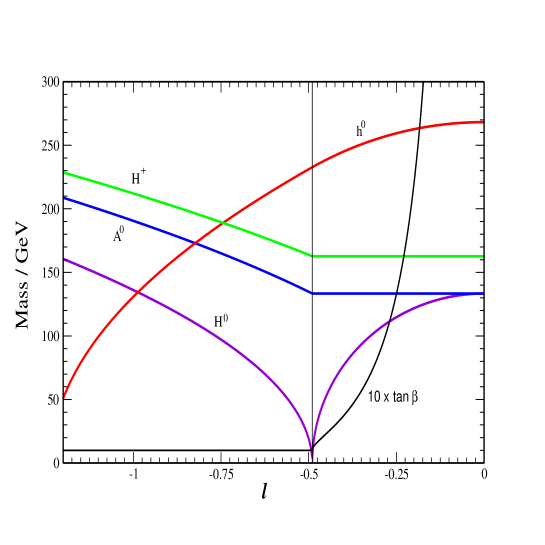
Figure 5: Higgs spectrum of example A as a function of the superpotential parameter $\ell$. Also shown is $\tan\beta$ (scaled by a factor 10).

In Fig. 5 we show a numerical example where both phases of the model are visible. We have fixed $\mu/M=0.6$, $e_{1}=-1.3$, $\tilde{m}/M=0.5$, $\alpha_{t}=3.0$, $\alpha_{1}\simeq\mu^{2}/\tilde{m}^{2}+\epsilon^{2}$ (with $0<\epsilon^{2}\ll 1$) and vary $\ell$. For each parameter choice, the overall mass scale $M$ is adjusted so as to get the right value of $v=246$ GeV. The closer $\alpha_{1}$ is to $\mu^{2}/\tilde{m}^{2}$ the larger $M/v$ can be. The figure shows the Higgs spectrum and the parameter $\tan\beta$ (scaled by a factor 10 for clarity) as a function of the coupling $\ell$. For $\ell\leq\ell_{0}$, with

$$\ell_{0}\equiv{M\over\mu}\left[{1\over 4}(g^{2}+g_{Y}^{2})+2\hat{e}_{1}{\mu^{2}\over M^{2}}\right]\ ,$$ (5.8)

the minimum lies at $\tan\beta=1$, while for $\ell>\ell_{0}$, $\tan\beta$ increases with $\ell$. For the choice of parameters used in this figure, $\ell_{0}\simeq-0.49$. The spectrum is continuous across the critical value $\ell_{0}$, although the mass of the ‘transverse’ Higgs, $H^{0}$, goes through zero, as was to be expected on general grounds for symmetric potentials. We see that, except in the neighbourhood of $\ell_{0}\simeq-0.49$ or for too negative values of $\ell$, the Higgs masses are sufficiently large to escape all current experimental bounds (which are also lower than usual due to singlet admixture, although this is typically a small effect). There is even a region of parameters for which $h^{0}$ is the heavier of the Higgses, beyond the usual limit of $m_{h^{0}}\stackrel{{\scriptstyle<}}{{{}_{\sim}}}200$ GeV [36] that applies in generic SUSY models only when they are perturbative up to the GUT scale.

One may also be interested in finding ${\cal O}(v^{2})$ corrections to the $T$ mass, which is $\alpha_{t}{\tilde{m}}^{2}$ at leading order. To do this, we should reconsider the potential prior to the elimination of $T$, including ${\cal O}(TH^{2})$ and ${\cal O}(T^{2}H^{2})$ terms. Taking also into account kinetic normalization, we get

$$m_{T}^{2}=\alpha_{t}{\tilde{m}}^{2}-{\alpha_{1}v^{2}\over 2M^{2}}\left[{\tilde{m}}^{2}(3\alpha_{t}-\alpha_{1})+\mu^{2}\left(1-4{\alpha_{1}\over\alpha_{t}}\right)\right]\,.$$ (5.9)

In the neutralino sector, the goldstino $\tilde{G}$ is mainly ${\tilde{T}}$. As a result of electroweak breaking, $\tilde{G}$ also has small components along Higgsinos and (for $\tan\beta\neq 1$) along gauginos, see eq. (4.31). The full $5\times 5$ neutralino mass matrix [including up to ${\cal O}(v^{2}/M)$ terms] is of the form (4.22) with $\kappa_{\omega}=0$, $\kappa_{1}=\ell Ms_{\beta}^{2}-e_{1}\mu s_{2\beta}$, $\kappa_{2}=\ell Mc_{\beta}^{2}-e_{1}\mu s_{2\beta}$,

$$M_{a}=\eta_{a}\tilde{m}\left(1-{\alpha_{1}v^{2}\over 2M^{2}}\right)-{\eta_{a}^{2}\alpha_{1}\mu v^{2}\over\alpha_{t}M^{2}}s_{2\beta}\ ,$$ (5.10)

and

$$\mu_{N}=\mu\left(1-{e_{1}v^{2}\over 2M^{2}}\right)+{\ell v^{2}\over 2M}s_{2\beta}\ .$$ (5.11)

The chargino sector is like in the MSSM, with a mass matrix of the form (4.34) and

$$\mu_{C}=\mu\left(1-{e_{1}v^{2}\over 4M^{2}}\right)+{\ell v^{2}\over 4M}s_{2\beta}\ .$$ (5.12)

Example B

Our general discussion and our previous example indicate that $T$-$H$ mixing effects generically arise after electroweak breaking, both in the scalar and in the fermion sector. This does not exclude the possibility to construct models where such mixing effects are absent and the goldstino remains a pure singlet (i.e. $\tilde{T}$), despite electroweak breaking. Here we present a simple model of this kind. We will see that when $\tilde{m}/M=\Lambda_{S}^{2}/M^{2}$ is negligible, the model becomes a special version of the MSSM with $\tan\beta=1$, and the $h^{0}$ Higgs boson has vanishing tree-level mass. When $\tilde{m}/M=\Lambda_{S}^{2}/M^{2}$ is sizeable, extra terms become important, which in particular make $h^{0}$ massive.

The superpotential, gauge kinetic functions and Kähler potential are chosen as

$$W=\Lambda_{S}^{2}T\ ,\;\;\;\;f_{ab}={\delta_{ab}\over g_{a}^{2}}\left(1+2{\eta_{a}\over M}T\right)$$ (5.13)

and

$$K = |T|^{2}+|H_{1}|^{2}+|H_{2}|^{2}-{\alpha_{t}\over 4M^{2}}|T|^{4}-{\gamma\over 2M^{4}}\left(|H_{1}|^{2}+|H_{2}|^{2}-{v^{2}\over 2}\right)^{2}|T|^{2}$$ (5.14)

$$+\left[|H_{1}|^{2}+|H_{2}|^{2}-(H_{1}\cdot H_{2}+{\rm h.c.})\right]\left[{\beta_{\mu}\over M}(T+\bar{T})-{\alpha\over M^{2}}|T|^{2}\right]\ ,$$

where all parameters are real. In this example $W$ is minimal, whereas $K$ is not. In fact, here the fields do not correspond to normal coordinates. In principle we could re-write the model in normal coordinates through field redefinitions, but such a coordinate change is not convenient in this case. Indeed, the model has been specifically designed in the above form in order to allow for a simple minimization of $V$, simple VEVs and a simple spectrum. In particular, some coefficients in $K$ have been adjusted in such a way that the minimization of $V$ can be performed exactly, so the perturbative procedure sketched in the previous sections is not necessary. The basic results can be summarized as follows.

i) The minimum lies at $\langle T\rangle=0$ and $\langle H_{1}^{0}\rangle=\langle H_{2}^{0}\rangle=v/2$, i.e. we have $\tan\beta=1$. The metric is canonical at the minimum: in particular, the components of $T$ and Higgs supermultiplets have no kinetic mixing.

ii) Supersymmetry is broken by the auxiliary component of $T$, with $\langle F^{T}\rangle=-\Lambda_{S}^{2}$, whereas $\langle F^{H_{i}}\rangle=0$ and $\langle D^{a}\rangle=0$. The SUSY-breaking scale is simply $\sqrt{F}=\Lambda_{S}$.

iii) The gauge symmetry is broken by the Higgs VEVs, and the $W$ and $Z$ masses have the usual expressions $M_{W}^{2}=g^{2}v^{2}/4$, $M_{Z}^{2}=(g^{2}+g_{Y}^{2})\ v^{2}/4$.

iv) In the fermion sector, $\tilde{T}$ does not mix with the other fields and coincides with the goldstino. The Higgsinos have mass $\mu=\beta_{\mu}\tilde{m}$ and the gauginos have mass $M_{a}=\eta_{a}\tilde{m}$. The breaking of the electroweak symmetry also generates mixed gaugino-Higgsino terms as usual. It is convenient to use the symmetric and antisymmetric combinations of neutral Higgsinos, i.e. $\tilde{H}_{A}^{0}\equiv(\tilde{H}_{1}^{0}-\tilde{H}_{2}^{0})/\sqrt{2}$ and $\tilde{H}_{S}^{0}\equiv(\tilde{H}_{1}^{0}+\tilde{H}_{2}^{0})/\sqrt{2}$. The field $\tilde{H}_{S}^{0}$ is a mass eigenstate and only $\tilde{H}_{A}^{0}$ is mixed with gauginos, because of $\tan\beta=1$. The neutralino and chargino mass matrices have standard form, apart from an extra zero eigenvalue corresponding to $\tilde{T}$.

v) In the spin-0 sector, $T$-$H$ mixing is absent as well. The complex field $T$, i.e. the scalar partner of $\tilde{T}$, has mass $m_{T}^{2}=\alpha_{t}\tilde{m}^{2}$. The Higgs boson spectrum can be summarized as follows:

$$G^{0}=\rm{Im}(H_{1}^{0}+\bar{H}_{2}^{0}) \rightarrow {\rm neutral\;Goldstone}$$ (5.15)

$$v+h^{0}=\rm{Re}(H_{1}^{0}+\bar{H}_{2}^{0}) \rightarrow m_{h}^{2}=\gamma v^{2}\tilde{m}^{2}/M^{2}$$ (5.16)

$$A^{0}=\rm{Im}(H_{1}^{0}-\bar{H}_{2}^{0}) \rightarrow m_{A}^{2}=2(\alpha+2\beta_{\mu}^{2})\tilde{m}^{2}$$ (5.17)

$$H^{0}=\rm{Re}(H_{1}^{0}-\bar{H}_{2}^{0}) \rightarrow m_{H}^{2}=m_{A}^{2}+M_{Z}^{2}$$ (5.18)

$$G^{-}=(H_{1}^{-}-\bar{H}_{2}^{-})/\sqrt{2} \rightarrow {\rm charged\;Goldstone}$$ (5.19)

$$H^{-}=(H_{1}^{-}+\bar{H}_{2}^{-})/\sqrt{2} \rightarrow m^{2}_{H^{\pm}}=m_{A}^{2}+M_{W}^{2}$$ (5.20)

where MSSM-type labels have been used. For $\gamma\tilde{m}^{2}/M^{2}\rightarrow 0$, this would be just the MSSM spectrum for $\tan\beta=1$. In this limit the electroweak symmetry is broken along a flat direction and the associated $h^{0}$ boson is massless. The $\gamma$ term has been added just to lift this flatness and obtain a nonzero $m_{h}$, which can easily be as large as $\sim 500$ GeV. Notice that the coupling $\gamma\tilde{m}^{2}/M^{2}$ plays the role of the coupling $\lambda$ in the SM Higgs potential, and we can obtain a realistic model if $\tilde{m}^{2}/M^{2}=\Lambda_{S}^{4}/M^{4}$ is sizeable.

It is straightforward to complete this model (and any other one) by introducing quark and lepton superfields, so that squarks and sleptons obtain ${\cal O}(\tilde{m})$ masses. Also notice that we can easily obtain a smooth decoupling limit in this model by keeping $v$ fixed and taking $\Lambda_{S}$ and $M$ large with $\Lambda_{S}/M$ fixed: in this limit part of the spectrum becomes heavy since $\tilde{m}$ becomes large and the low-energy theory is just the SM, since the light particles are only the SM ones, plus the goldstino, which is decoupled.

Although the results we have obtained are exact, it is instructive to expand the full Higgs potential up to ${\cal O}(H^{4})$-terms to make contact with two-Higgs-doublet models. If we do this, we obtain the mass parameters

$$m_{1}^{2}=m_{2}^{2}=(\alpha+2\beta_{\mu}^{2})\tilde{m}^{2}-{1\over 2}\gamma{\tilde{m}^{2}\over M^{2}}v^{2}\ ,\;\;\;\;m_{3}^{2}=-(\alpha+2\beta_{\mu}^{2})\tilde{m}^{2}\ ,$$ (5.21)

where we neglect ${\cal O}(v^{4}\tilde{m}^{2}/M^{4})$ terms, and quartic couplings

$$\lambda_{1}=\lambda_{2} = {1\over 4}(g^{2}+g_{Y}^{2})+[\gamma+2(\alpha+2\beta_{\mu}^{2})^{2}]{\tilde{m}^{2}\over M^{2}}\ ,$$

$$\lambda_{3} = {1\over 4}(g^{2}-g_{Y}^{2})+[\gamma+2(\alpha+2\beta_{\mu}^{2})^{2}]{\tilde{m}^{2}\over M^{2}}\ ,$$

$$\lambda_{4} = -{1\over 2}g^{2}+2(\alpha+2\beta_{\mu}^{2})^{2}{\tilde{m}^{2}\over M^{2}}\ ,$$

$$\lambda_{5}=-\lambda_{6}=-\lambda_{7} = 2(\alpha+2\beta_{\mu}^{2})^{2}{\tilde{m}^{2}\over M^{2}}\ ,$$ (5.22)

where we neglect ${\cal O}(v^{2}\tilde{m}^{2}/M^{4})$ terms. This example would thus correspond in Fig. 1 to point B. If we insert these expressions in the general formulae for the 2HDM Higgs spectrum (see Appendix A), we formally recover the results in Eqs. (5.15)-(5.20).

We conclude this section by showing an illustrative example of goldstino interaction with a Higgs-Higgsino pair. Although we have not discussed this topic before, we stress that these couplings are in general present, i.e. they are not specific of the model under consideration, and could be phenomenologically relevant for the decay of a Higgsino into a goldstino and a Higgs boson (see e.g. [10]) or, viceversa, for the decay of a Higgs boson into a goldstino-Higgsino pair (see e.g. [37]). We use the above model only to check that such couplings have the standard (model-independent) form $\Delta m^{2}/F$ [8], where $\Delta m^{2}$ is the mass splitting of the fermion-sfermion pair under consideration. To avoid the complications of mixing effects, we focus on the cubic interactions of the goldstino (i.e. $\tilde{T}$) with the Higgs boson $h^{0}$ and the Higgsino $\tilde{H}_{S}^{0}$, which are mass eigenstates and belong to the same supermultiplet, i.e. $(H_{1}^{0}+H_{2}^{0})/\sqrt{2}$. The Lagrangian contains both non-derivative and derivative interactions of that type. Using the fermion equations of motion we can write the derivative ones in non-derivative form and combine them with the other ones. Once this is done, the effective on-shell interaction can be written in the simple form

$$-{1\over\sqrt{2}}{m_{h}^{2}-\mu^{2}\over\Lambda_{S}^{2}}\,h^{0}\tilde{H}_{S}^{0}\tilde{T}+{\rm h.c.}\,,$$ (5.23)

which is the expected result.

6 Electroweak breaking and two-goldstino interactions

The effective interactions of one goldstino with a fermion-boson pair, which are uniquely determined by supercurrent conservation, can be expressed in terms of the corresponding masses (and mixing angles) and of the SUSY-breaking scale [8]. In the last example of the previous section we have checked that the model-independent form of such couplings is respected also in the Higgs sector, where electroweak breaking takes place. We devote this section to study the impact of electroweak breaking on the effective interactions that involve two goldstinos. We recall that even if the available experimental energy is not sufficient to produce the SUSY partners of SM particles, SUSY can still be probed in processes involving SM particles and two goldstinos. Since the corresponding amplitudes are strongly constrained by general goldstino properties, by comparison with experiments one can obtain useful information on the SUSY-breaking scale [14, 15, 19]. We would like to study how the coefficients of such interactions are affected by electroweak breaking. To this purpose, we resort to the general framework of sect. 2. So our starting point is a general effective theory with linearly realized SUSY and $SU(3)\times SU(2)\times U(1)_{Y}$ gauge group. The chiral supermultiplets include the MSSM ones and singlets (in the simplest case, just one $T$ field). In the limit of unbroken $SU(2)\times U(1)$, SUSY can only be broken by the $F$-terms of the singlets: in this case, the goldstino and its bosonic partners belong to the singlet sector. Upon $SU(2)\times U(1)$ breaking, SUSY breaking can receive additional contributions from non-vanishing values of $\langle F^{H_{1}^{0}}\rangle$, $\langle F^{H_{2}^{0}}\rangle$, $\langle D^{3}\rangle$ and $\langle D^{Y}\rangle$. If this is the case, also the neutral Higgsinos and gauginos have components along the goldstino. Moreover, the neutral Higgs bosons and the $Z$ boson are (partly) bosonic partners of the goldstino. This implies that such bosons can have non-vanishing on-shell couplings to goldstino bilinears, as we will check below. More precisely, in the following we will discuss the effective interactions between two goldstinos and: i) a $Z$ boson; ii) a Higgs boson; iii) two SM fermions (leptons or quarks).

We recall that the total amount of SUSY breaking is parametrized by $F^{2}\equiv\langle V_{F}+V_{D}\rangle$, as in eq. (2.3). The indices $i,j,\ldots$ below will run over electrically neutral chiral supermultiplets, which can have non-vanishing VEVs in their lowest or auxiliary components (i.e. $T$, $H_{1}^{0}$ and $H_{2}^{0}$, which will be treated on the same footing). We also emphasize that, in contrast to our approach in other sections, throughout our derivations below we will not expand the basic functions in powers of Higgs fields, both for the sake of generality and for technical convenience.

6.1 $Z$–goldstino–goldstino

A connection between the $Z$-goldstino-goldstino coupling and non-vanishing electroweak $D$-terms was found in [15], in the framework of non-linearly realized SUSY. Here we present an alternative derivation of such a coupling, starting from a general effective Lagrangian with linearly realized SUSY. Let us consider the coupling of a generic neutral gauge boson $A^{a}_{\mu}=\{W^{3}_{\mu},B_{\mu}\}$ to fermion bilinears $\bar{\psi}^{\bar{\imath}}\bar{\sigma}^{\mu}\psi^{j}$, where the fermions belong to electrically neutral chiral multiplets $(\varphi^{i},\psi^{i},F^{i})$, with $t^{a}_{i}$ denoting the weak isospin or the hypercharge. After selecting the goldstino components of the fermions ($\psi^{i}\supset\tilde{G}\langle F^{i}\rangle/F$), we obtain

$$-{g_{a}\over F^{2}}\langle\bar{F}^{\bar{\imath}}\left(K_{\bar{\imath}j}t^{a}_{j}+K_{\bar{\imath}j\ell}t^{a}_{\ell}\varphi^{\ell}\right)F^{j}\rangle A^{a}_{\mu}\tilde{\bar{G}}\bar{\sigma}^{\mu}\tilde{G}\ ,$$ (6.1)

where $g_{a}\equiv\langle(Ref_{a})^{-1}\rangle$ is the gauge coupling of $A^{a}_{\mu}$. We recall that, upon electroweak breaking, the goldstino can also have components along neutral gauginos, for non-vanishing $\langle D^{a}\rangle$. However, such components do not contribute to the coupling of $A^{a}_{\mu}$ to goldstino bilinears. This could give the impression that the $Z$-goldstino-goldstino coupling is only determined by $F$-breaking, with electroweak $D$-breaking playing no role. However, a closer inspection reveals that the coupling is non zero only if $\langle D^{a}\rangle\neq 0$. Indeed, the VEVs $\langle F^{i}\rangle$ and $\langle D^{a}\rangle$ are related by the extremum conditions of the scalar potential. Using these conditions and the constraints from gauge invariance we can write the coupling above in terms of $\langle D^{a}\rangle$:

$${1\over 2F^{2}}\langle D^{a}\rangle M^{2}_{ab}\,A^{b}_{\mu}\tilde{\bar{G}}\bar{\sigma}^{\mu}\tilde{G}\ ,$$ (6.2)

where $M^{2}_{ab}$ is the gauge boson mass matrix and $\langle D^{a}\rangle=-g_{a}\langle K_{j}t_{j}^{a}\varphi^{j}\rangle$. Therefore the coupling of a $Z$ boson to a goldstino pair is

$${\langle D_{Z}\rangle M^{2}_{Z}\over 2F^{2}}Z_{\mu}\tilde{\bar{G}}\bar{\sigma}^{\mu}\tilde{G}\ ,$$ (6.3)

where $\langle D_{Z}\rangle=\langle c_{w}D^{3}-s_{w}D^{Y}\rangle\simeq-(M_{Z}^{2}/g_{Z})\cos 2\beta$ [with $g_{Z}\equiv\sqrt{g^{2}+g_{Y}^{2}}=e/(s_{w}c_{w})$]. The associated decay width is

$$\Gamma(Z\rightarrow\tilde{G}\tilde{G})={\langle D_{Z}\rangle^{2}M_{Z}^{5}\over 96\pi F^{4}}\simeq\cos^{2}2\beta\left({200\,{\rm GeV}\over\sqrt{F}}\right)^{8}{\rm MeV}\ ,$$ (6.4)

in agreement with [15]. The on-shell equivalence of the operator (6.2) above to the one found in [15], i.e. ${\langle D_{a}\rangle\over 2F^{2}}F^{a}_{\mu\nu}\partial^{\mu}\tilde{\bar{G}}\bar{\sigma}^{\nu}\tilde{G}+{\rm h.c.}$, can also be checked through the goldstino and gauge boson equations of motion. By doing this, in fact, the latter operator can easily be converted into the operator (6.2).

6.2 Higgs-goldstino-goldstino

The coupling of a neutral scalar particle to two (on-shell) goldstinos can be derived from the field-dependent neutral-fermion mass matrix. We can take eq. (2.5) without VEVs, expand the coefficients of $\lambda^{a}\lambda^{b}$, $\lambda^{a}\psi^{j}$, $\psi^{i}\psi^{j}$ to linear order in the scalar fluctuations ($\delta\varphi^{i}=\varphi^{i}-\langle\varphi^{i}\rangle$) and select the goldstino components of the fermion fields, eq. (2.6). The resulting expression is quite involved: it depends on $\langle F^{i}\rangle$, $\langle D^{a}\rangle$ and several derivatives of $K$, $W$ and $f_{ab}$. However, by using once again the extremum conditions of the scalar potential and gauge invariance, the coefficients of the scalar-goldstino-goldstino interactions can be expressed in terms of the scalar masses and $\langle F^{i}\rangle$. The result reads:

$${1\over 2F^{2}}\langle F^{i}\rangle\left(M^{2}_{i\bar{\jmath}}\,\delta\bar{\varphi}^{\bar{\jmath}}+M^{2}_{ij}\,\delta{\varphi}^{j}\right)\tilde{G}\tilde{G}+{\rm h.c.}\ ,$$ (6.5)

where $M^{2}_{i\bar{\jmath}}\equiv\langle V_{i\bar{\jmath}}\rangle$ and $M^{2}_{ij}\equiv\langle V_{ij}\rangle$ are the elements of the scalar mass matrix. Notice the similarity of the boson-goldstino-goldstino interactions in (6.5) with those in (6.2): in both cases the coefficients are proportional to the corresponding boson masses, to the VEVs of the associated auxiliary fields and to $1/F^{2}$. In the limit in which SUSY is only broken by the F-term $\langle F^{T}\rangle$ of a singlet superfield $T$ and the $T$-scalars have neither kinetic nor mass mixing with the Higgses, then only the $T$-scalars couple to two on-shell goldstinos and (6.5) reduces to known results [38, 4]. Electroweak breaking, however, generically induces also non-vanishing values of $\langle F^{H_{i}^{0}}\rangle$ and $T$-$H$ mixing, so also neutral Higgs bosons can couple to goldstino bilinears. The typical size of such couplings is ${\cal O}(v\mu M_{H}^{2}/F^{2})$, where $M_{H}$ denotes the Higgs boson mass. More specific expressions can be obtained in any given model. Thus a neutral Higgs boson can decay invisibly into a goldstino pair. We recall that, in the limiting case of a sizeable invisible width, also the branching fractions of the visible channels are indirectly modified.

6.3 Goldstino interactions with matter fermions

We now consider (two goldstino)-(two fermion) effective interactions. We recall that, although the leading energy- and $F$-dependence of such interactions is completely fixed, the presence of (non-universal) model dependent coefficients is allowed by general results on non-linearly realized SUSY [39, 40]. This has also been confirmed in specific string (brane) constructions [41]. In the framework of effective Lagrangians with linearly realized SUSY, a possible source of such parameters is the presence of $D$-type SUSY breaking (besides $F$-type SUSY breaking). Indeed, in this case the effective (two goldstino)-(two fermion) interactions depend on the fermion quantum numbers under the gauge group with non vanishing $D$ terms, because of the exchange contribution due to the associated massive gauge bosons [42, 11, 19]. A physically relevant example of such a situation is precisely the case of a SUSY effective Lagrangian with gauge group $SU(3)\times SU(2)\times U(1)$ spontaneously broken to $SU(3)\times U(1)_{em}$, since the electroweak $D$-terms can have non-vanishing VEVs. Therefore, let us consider this case in more detail.

Let $f$ denote a Weyl fermion in the lepton/quark sector, with isospin $t_{f}^{3}$ and electric charge $Q_{f}$. The (on-shell) interactions involving two goldstinos and two $f$-type fermions arise from three sources: sfermion exchange, $Z$ exchange and contact interaction. We recall that the sfermion mass has two contributions (from $V_{F}$ and $V_{D}$):

$$\tilde{m}^{2}_{f}=(\tilde{m}^{2}_{f})_{F}+(\tilde{m}^{2}_{f})_{D}=\langle\bar{F}^{\bar{\imath}}(-\log K_{\bar{f}f})_{\bar{\imath}j}F^{j}\rangle-g_{Z}\langle D_{Z}\rangle Q^{Z}_{f}\ ,$$ (6.6)

where $Q^{Z}_{f}\equiv t_{f}^{3}-Q_{f}s_{w}^{2}+\langle(\log K_{\bar{f}f})_{j}t_{j}^{3}\varphi^{j}\rangle$ and $K_{\bar{f}f}$ denotes the Kähler metric of the supermultiplet $(\tilde{f},f)$. The relevant interaction terms, including the one in (6.3), are:

$$\left[{\langle D_{Z}\rangle M^{2}_{Z}\over 2F^{2}}\tilde{\bar{G}}\bar{\sigma}^{\mu}\tilde{G}-g_{Z}Q^{Z}_{f}\bar{f}\bar{\sigma}^{\mu}f\right]Z_{\mu}+{\tilde{m}^{2}_{f}\over F}\left(\tilde{f}^{*}f\tilde{G}+{\rm h.c.}\right)-{(\tilde{m}^{2}_{f})_{F}\over 2F^{2}}(\bar{f}\bar{\sigma}^{\mu}f)(\tilde{\bar{G}}\bar{\sigma}_{\mu}\tilde{G}),$$ (6.7)

where all fields are canonically normalized. An important consequence of the close connection between mass spectrum and goldstino couplings, which is manifest in eq. (6.7), is that the different contributions to (two goldstino)-(two fermion) interactions cancel against each other at zero momentum, as they should. The first non-vanishing terms in the momentum expansion (i.e. the leading terms for energies smaller than $M_{Z}$ and $\tilde{m}_{f}$) contain two derivatives and have the form

$$-{1\over F^{2}}\left[(\bar{f}\tilde{\bar{G}})\Box(f\tilde{G})+{1\over 2}c_{f}(\bar{f}\bar{\sigma}^{\mu}f)\Box(\tilde{\bar{G}}\bar{\sigma}_{\mu}\tilde{G})\right]$$ (6.8)

where $c_{f}$ has the specific value $c_{f}=g_{Z}\langle D_{Z}\rangle Q^{Z}_{f}/M_{Z}^{2}\simeq-(t_{f}^{3}-Q_{f}s_{w}^{2})\cos 2\beta$. The result in (6.8) is consistent with the general form allowed by non-linearly realized SUSY. If one is interested in (two goldstino)-(two fermion) interactions at higher energies, the local operators in (6.8) should be generalized to include the full effect of $\tilde{f}$ and $Z$ propagators: this amounts to replace $\Box\rightarrow\Box(1+\Box/\tilde{m}_{f}^{2})^{-1}$ in the first operator and $\Box\rightarrow\Box(1+\Box/M_{Z}^{2})^{-1}$ in the second operator.

Let us focus on the process $f\bar{f}\rightarrow\tilde{G}\tilde{G}$ at $s\ll\tilde{m}^{2}_{f}$ and consider the effect of the $Z$ threshold. The cross-section is

$$\sigma(f\bar{f}\rightarrow\tilde{G}\tilde{G}) = {s^{3}\over 80\pi F^{4}}\left[1+{5\over 2}(t_{f}^{3}-Q_{f}s_{w}^{2})\cos 2\beta\;A(s/M_{Z}^{2})\right.$$ (6.9)

$$\left.+{5\over 3}(t_{f}^{3}-Q_{f}s_{w}^{2})^{2}\cos^{2}2\beta\;B(s/M_{Z}^{2})\right]$$

where $A(y)\equiv(1-y)B(y)\equiv(1-y)/[(1-y)^{2}+\epsilon^{2}y^{2}]$ and $\epsilon=\Gamma_{Z}/M_{Z}$ takes into account the finite $Z$ width. When $\langle D_{Z}\rangle=0$ (i.e. $\cos 2\beta=0$), only the first term in eq. (6.9) [or in (6.8)] is relevant and the cross section reduces to $\sigma\simeq s^{3}/(80\pi F^{4})$ [39]. For $\langle D_{Z}\rangle\neq 0$, however, this simple result only holds above the $Z$ threshold, i.e. for $M_{Z}^{2}\ll s\ll\tilde{m}^{2}_{f}$, where the second and third terms in eq. (6.9) are suppressed [$A(y)\sim-1/y$ and $B(y)\sim 1/y^{2}$ for $y\gg 1$]. On the other hand, such terms become dominant in the resonance region. Below resonance, all three terms in eq. (6.9) contribute with comparable weight [$A(0)=B(0)=1$]. It is straightfoward to extend these results to a $SM$ fermion ${\cal F}$ with both helicity components, i.e. $SU(2)$ doublet component $f$ and singlet component $\bar{f^{c}}$. The unpolarized cross section for ${\cal F}\bar{\cal F}\rightarrow\tilde{G}\tilde{G}$ is easily inferred from eq. (6.9):

$$\sigma_{\rm unp}({\cal F}\bar{\cal F}\rightarrow\tilde{G}\tilde{G}) = {s^{3}\over N\,160\pi F^{4}}\left[1+{5\over 4}\,t_{f}^{3}\cos 2\beta\;A(s/M_{Z}^{2})\right.$$ (6.10)

$$\left.+{5\over 6}\left({1\over 4}-2\,t_{f}^{3}Q_{f}s_{w}^{2}+2\,Q_{f}^{2}s_{w}^{4}\right)\cos^{2}2\beta\;B(s/M_{Z}^{2})\right]$$

where $N=1\,(3)$ for charged leptons (quarks). We also recall that, in order to obtain a visible signal at colliders, the goldstino pair should be accompanied for instance by a photon or a gluon, as in $e^{+}e^{-}\rightarrow\tilde{G}\tilde{G}\gamma$, $Q\bar{Q}\rightarrow\tilde{G}\tilde{G}\gamma$, $Q\bar{Q}\rightarrow\tilde{G}\tilde{G}g$ (see e.g. [14]). As an alternative to a full computation, approximate expressions for the cross section of such five-particle processes can be obtained by convoluting the above four-particle cross section with the radiator functions that describe initial state radiation. Then the kinematical variable $s$ in eq. (6.10) would be related to the analogous quantity $S$ of the five-particle process through $s=S(1-x)$, where $x$ is the energy fraction taken away by the photon or the gluon.

7 Summary and conclusions

In recent years there has been an intense activity on supersymmetric models in which the scales of SUSY breaking ($\sqrt{F}$) and mediation ($M$) are close to the electroweak scale. These include models of extra dimensions (warped or not) with low fundamental scale and, more generally, scenarios in which the low-energy supersymmetric effective theory is obtained by integrating out physics at energy scales not far from the TeV scale. In all these cases the usual MSSM, where the effects of SUSY breaking in the observable sector are encoded in a set of soft SUSY-breaking terms of size ${\cal O}(F/M)$, may not give an accurate enough effective description. Additional effects can be relevant, in particular interactions of the goldstino sector with the observable sector and non-negligible contributions to ‘hard-breaking’ terms, such as ${\cal O}(F^{2}/M^{4})$ contributions to quartic Higgs couplings. In fact, the latter contributions can compete with (and may take over) the usual ($D$-term induced) MSSM quartic Higgs couplings, giving rise to a quite unconventional Higgs sector phenomenology, as already observed in [7]. The main purpose of this paper has been to study in detail the latter aspect, i.e. to perform a general analysis of the Higgs sector and the breaking of SUSY and electroweak symmetry in this type of models. To do this, we have used a model-independent approach based on a general effective Lagrangian, in which the MSSM superfields are effectively coupled to a singlet superfield, assumed to be the main source of SUSY breaking. Our main results can be summarized as follows:

• Rather than the usual MSSM potential, the Higgs potential resembles that of a two-Higgs-doublet model (2HDM), where the quadratic and quartic couplings can be traced back to the original couplings in the effective superpotential and Kähler potential. However, there are still some differences, e.g. the presence of derivative couplings besides the non-derivative ones described by the scalar potential. Moreover, the scalar sector also contains an extra complex degree of freedom, which comes from the singlet supermultiplet. This scalar field can have non-negligible interactions with the Higgs fields, and could also mix with them as a result of electroweak breaking.

• The presence of extra quartic couplings that may be larger than the usual ones opens novel opportunities for electroweak breaking. The breaking process is effectively triggered at tree-level and presents important differences with the usual radiative mechanism. Electroweak breaking can occur in a much wider region of parameter space, i.e. for values of the low-energy mass parameters that are normally forbidden. For instance, $m_{H_{1}}^{2}$ and $m_{H_{2}}^{2}$ are allowed to be both negative. Another unconventional situation, now allowed, is the case in which $m_{H_{1}}^{2}$ and $m_{H_{2}}^{2}$ are equal and positive, and electroweak breaking is driven by $m_{3}^{2}\ H_{1}\cdot H_{2}$. This breaking is natural, since the latter term is the only off-diagonal bilinear coupling among MSSM fields (with R-parity conserved), so $SU(2)_{L}\times U(1)_{Y}$ is the only symmetry that can be broken when all scalar masses are positive. A further advantage of the extra quartic couplings is that their presence may reduce the amount of tuning necessary to get the correct Higgs VEVs.

• The spectrum of the Higgs sector is also dramatically changed, and the usual MSSM mass relations are easily violated. In particular, the new quartic couplings allow the lightest Higgs field to be much heavier ($\lower 3.01385pt\hbox{$\;\stackrel{{\scriptstyle\textstyle<}}{{\sim}}\;$}500$ GeV) than in usual supersymmetric scenarios. Moreover, this field could have a substantial singlet component, modifying its properties.

• Departures from the usual MSSM results also appear in the chargino and neutralino mass matrices, where the effective operators induce some corrections after electroweak breaking. Moreover, the neutralino sector also includes the goldstino. This is a singlet in the limit of unbroken electroweak symmetry, but generically (although not necessarily) also acquires Higgsino and gaugino components after electroweak breaking.

• After giving a general derivation and discussion of the above properties, we have illustrated them in two simple examples, analyzing in each case the Higgs potential, the electroweak breaking process, the Higgs masses and the neutralino and chargino spectra.

• Finally, we have analysed the role of electroweak breaking in processes in which SM particles could emit a goldstino pair, such as fermion-antifermion annihilations and the invisible decays of $Z$ and Higgs bosons. We recall that such processes may offer an important window to SUSY, especially if other superparticles are not experimentally accessible.

In conclusion, it is clear that many features of the conventional MSSM Higgs sector and related ones can be significantly changed in scenarios with low-scale SUSY breaking (examples of this are the mechanism of the electroweak breaking and the mass of the lightest Higgs). This potentially offers new ways to overcome traditional difficulties of the MSSM as well as new prospects for the detection of SUSY in future experiments.

Appendix A

This Appendix deals with a subclass of quartic two-Higgs-doublet potentials: those which have real parameters and are invariant under a symmetry that exchanges the two doublets. The mass parameters and the quartic couplings of such a potential are subject to the restrictions $m_{1}^{2}=m_{2}^{2}$, $\lambda_{1}=\lambda_{2}$ and $\lambda_{6}=\lambda_{7}$, i.e. the potential has the form

$$V(H_{1},H_{2}) = m_{1}^{2}(|H_{1}|^{2}+|H_{2}|^{2})+m_{3}^{2}(H_{1}\cdot H_{2}+{\rm h.c.})$$ (A.1)

$$+ {1\over 2}\lambda_{1}(|H_{1}|^{4}+|H_{2}|^{4})+\lambda_{3}|H_{1}|^{2}|H_{2}|^{2}+\lambda_{4}|H_{1}\cdot H_{2}|^{2}$$

$$+ {1\over 2}\lambda_{5}\left[(H_{1}\cdot H_{2})^{2}+{\rm h.c.}\right]+\lambda_{6}(|H_{1}|^{2}+|H_{2}|^{2})(H_{1}\cdot H_{2}+{\rm h.c.}).$$

A special case of symmetric potentials are those invariant under $SU(2)_{L}\times SU(2)_{R}$. Such potentials only depend on the quantities $|H_{1}|^{2}+|H_{2}|^{2}$ and $H_{1}\cdot H_{2}$, so the further condition $\lambda_{1}=\lambda_{3}$ holds for them.

If a symmetric potential of the form (A.1) admits a minimum with nonvanishing Higgs VEVs, such a minimum could either preserve ($|\tan\beta|=1$) or break spontaneously ($|\tan\beta|\neq 1$) the discrete symmetry that exchanges the two doublets. We will now present the conditions under which the former or the latter case is realized, and give explicit formulae for the Higgs boson masses. We anticipate that, in the special case of $SU(2)_{L}\times SU(2)_{R}$ invariant potentials, only the case $|\tan\beta|=1$ can be realized. For later convenience, we introduce the following abbreviation: $\tilde{\lambda}\equiv(1/2)(-\lambda_{1}+\lambda_{3}+\lambda_{4}+\lambda_{5})$.

Minima with $|\tan\beta|=1$

The conditions to have a minimum with $\tan\beta=s=\pm 1$ are:

$$m_{1}^{2}+sm_{3}^{2} < 0\ ,$$ (A.2)

$$\lambda_{1}+\tilde{\lambda}+2s\lambda_{6} > 0\ ,$$ (A.3)

$$(\tilde{\lambda}+s\lambda_{6})m_{1}^{2} > (\lambda_{1}+s\lambda_{6})sm_{3}^{2}\ ,$$ (A.4)

$$(\lambda_{5}+s\lambda_{6})m_{1}^{2} > (\lambda_{1}+\tilde{\lambda}-\lambda_{5}+s\lambda_{6})sm_{3}^{2}\ ,$$ (A.5)

$$(\lambda_{4}+\lambda_{5}+2s\lambda_{6})m_{1}^{2} > (\lambda_{1}+\lambda_{3}+2s\lambda_{6})sm_{3}^{2}\ .$$ (A.6)

The value of $v^{2}\equiv 2\langle|H_{1}^{0}|^{2}+|H_{2}^{0}|^{2}\rangle$ is

$$v^{2}={-2(m_{1}^{2}+sm_{3}^{2})\over\lambda_{1}+\tilde{\lambda}+2s\lambda_{6}}\ .$$ (A.7)

The mass of the Higgs field along the VEV direction is

$$m_{h}^{2}=(\lambda_{1}+\tilde{\lambda}+2s\lambda_{6})\,v^{2}\ .$$ (A.8)

The remaining Higgs boson masses are

$$m_{H}^{2} = 2m_{1}^{2}+(\lambda_{1}+s\lambda_{6})v^{2}\,=\,-2sm_{3}^{2}-(\tilde{\lambda}+s\lambda_{6})\,v^{2}\ ,$$ (A.9)

$$m_{A}^{2} = 2m_{1}^{2}+(\lambda_{1}+\tilde{\lambda}-\lambda_{5}+s\lambda_{6})\,v^{2}\,=\,-2sm_{3}^{2}-(\lambda_{5}+s\lambda_{6})\,v^{2}\ ,$$ (A.10)

$$m_{H^{\pm}}^{2} = 2m_{1}^{2}+\left[{1\over 2}(\lambda_{1}+\lambda_{3})+s\lambda_{6}\right]v^{2}=-2sm_{3}^{2}-\left[{1\over 2}(\lambda_{4}+\lambda_{5})+s\lambda_{6}\right]v^{2}.$$ (A.11)

Minima with $|\tan\beta|\neq 1$

The conditions to have a minimum with $|\tan\beta|\neq 1$ are:

$$m_{1}^{2}-|m_{3}^{2}| < 0\ ,$$ (A.12)

$$\lambda_{3}>\lambda_{1} > 0\ ,$$ (A.13)

$$\lambda_{1}\tilde{\lambda} > \lambda_{6}^{2}\ ,$$ (A.14)

$$\tilde{\lambda} > \lambda_{5}\ ,$$ (A.15)

$$\lambda_{6}m_{3}^{2}-\tilde{\lambda}m_{1}^{2} > |\lambda_{6}m_{1}^{2}-\lambda_{1}m_{3}^{2}|\ .$$ (A.16)

The values of $v^{2}\equiv 2\langle|H_{1}^{0}|^{2}+|H_{2}^{0}|^{2}\rangle$ and $\tan\beta\equiv\langle H_{2}^{0}/H_{1}^{0}\rangle$ are determined by

$$v^{2}={2(\lambda_{6}m_{3}^{2}-\tilde{\lambda}m_{1}^{2})\over\tilde{\lambda}\lambda_{1}-\lambda_{6}^{2}}\ ,\;\;\;\sin 2\beta={\lambda_{6}m_{1}^{2}-\lambda_{1}m_{3}^{2}\over\lambda_{6}m_{3}^{2}-\tilde{\lambda}m_{1}^{2}}\ .$$ (A.17)

The CP-even Higgs mass matrix, projected on the VEV direction ($h_{\parallel}$) and on the orthogonal one ($h_{\perp}$), reads:

$$\langle h_{\parallel}|{\cal M}^{2}|h_{\parallel}\rangle = (\lambda_{1}+\tilde{\lambda}\sin^{2}2\beta+2\lambda_{6}\sin 2\beta)\,v^{2}\ ,$$ (A.18)

$$\langle h_{\perp}|{\cal M}^{2}|h_{\perp}\rangle = (\tilde{\lambda}\cos^{2}2\beta)\,v^{2}\ ,$$ (A.19)

$$\langle h_{\parallel}|{\cal M}^{2}|h_{\perp}\rangle = (\tilde{\lambda}\sin 2\beta+\lambda_{6})\cos 2\beta\,v^{2}\ .$$ (A.20)

These imply the following bounds on the masses of the CP-even Higgs bosons:

$${\mathrm{m}in}\{m_{h}^{2},m_{H}^{2}\}\leq\langle h_{\parallel}|{\cal M}^{2}|h_{\parallel}\rangle\leq{\mathrm{m}ax}\{m_{h}^{2},m_{H}^{2}\}\ ,$$ (A.21)

$${\mathrm{m}in}\{m_{h}^{2},m_{H}^{2}\}\leq\langle h_{\perp}|{\cal M}^{2}|h_{\perp}\rangle\leq{\mathrm{m}ax}\{m_{h}^{2},m_{H}^{2}\}\ .$$ (A.22)

The CP-odd and charged Higgs masses are

$$m_{A}^{2} = {1\over 2}(-\lambda_{1}+\lambda_{3}+\lambda_{4}-\lambda_{5})v^{2}\,=\,(\tilde{\lambda}-\lambda_{5})\,v^{2}\ ,$$ (A.23)

$$m_{H^{\pm}}^{2} = {1\over 2}(-\lambda_{1}+\lambda_{3})\,v^{2}\,=\,\left[\tilde{\lambda}-{1\over 2}(\lambda_{4}+\lambda_{5})\right]v^{2}\ .$$ (A.24)

In particular notice that, in order to have a minimum with $|\tan\beta|\neq 1$ and positive $m_{H^{\pm}}^{2}$, a symmetric potential has to fulfil the condition $\lambda_{3}-\lambda_{1}>0$. This is not satisfied by $SU(2)_{L}\times SU(2)_{R}$ invariant potentials: in this case a non-trivial minimum necessarily has $|\tan\beta|=1$. The same conclusion holds in those supersymmetric models in which $SU(2)_{L}\times SU(2)_{R}$ is preserved by the Kähler potential (before inserting the $U(1)_{Y}$ vector superfield) and is only broken by the hypercharge coupling $g^{\prime}$: in such a case $\lambda_{3}-\lambda_{1}=-g^{\prime 2}/2<0$, so a non-trivial minimum necessarily has $|\tan\beta|=1$.

References

- [1] H. P. Nilles, Phys. Rept. 110 (1984) 1; H. E. Haber and G. L. Kane, Phys. Rept. 117 (1985) 75; S. P. Martin [hep-ph/9709356]; S. Weinberg, “The Quantum Theory Of Fields. Vol. 3: Supersymmetry,” Cambridge, UK: Univ. Pr. (2000).
- [2] G. F. Giudice and R. Rattazzi, Phys. Rept. 322 (1999) 419 [hep-ph/9801271].
- [3] T. Gherghetta and A. Pomarol, Nucl. Phys. B 586 (2000) 141 [hep-ph/0003129] and Nucl. Phys. B 602 (2001) 3 [hep-ph/0012378]; J. Bagger, D. Nemeschansky and R. J. Zhang, JHEP 0108 (2001) 057 [hep-th/0012163]; M. A. Luty and R. Sundrum, Phys. Rev. D 64 (2001) 065012 [hep-th/0012158]; A. Falkowski, Z. Lalak and S. Pokorski, Nucl. Phys. B 613 (2001) 189 [hep-th/0102145]; D. Marti and A. Pomarol, Phys. Rev. D 64 (2001) 105025 [hep-th/0106256]; J. A. Casas, J. R. Espinosa and I. Navarro, Nucl. Phys. B 620 (2002) 195 [hep-ph/0109127].
- [4] A. Brignole, F. Feruglio and F. Zwirner, Nucl. Phys. B 501 (1997) 332 [hep-ph/9703286].
- [5] S. Dimopoulos and H. Georgi, Nucl. Phys. B 193 (1981) 150; L. Girardello and M. T. Grisaru, Nucl. Phys. B 194 (1982) 65.
- [6] K. Harada and N. Sakai, Prog. Theor. Phys. 67 (1982) 1877; K. Inoue, A. Kakuto, H. Komatsu and S. Takeshita, Prog. Theor. Phys. 68 (1982) 927 [Erratum-ibid. 70 (1983) 330]; D. R. Jones, L. Mezincescu and Y. P. Yao, Phys. Lett. B 148 (1984) 317; L. J. Hall and L. Randall, Phys. Rev. Lett. 65 (1990) 2939; I. Jack and D. R. Jones, Phys. Lett. B 457 (1999) 101 [hep-ph/9903365]; F. Borzumati, G. R. Farrar, N. Polonsky and S. Thomas, Nucl. Phys. B 555 (1999) 53 [hep-ph/9902443]; S. P. Martin, Phys. Rev. D 61 (2000) 035004 [hep-ph/9907550].
- [7] N. Polonsky and S. Su, Phys. Lett. B 508 (2001) 103 [hep-ph/0010113] and Phys. Rev. D 63 (2001) 035007 [hep-ph/0006174]; N. Polonsky, Nucl. Phys. Proc. Suppl. 101 (2001) 357 [hep-ph/0102196].
- [8] P. Fayet, Phys. Lett. B 70 (1977) 461.
- [9] R. Casalbuoni, S. De Curtis, D. Dominici, F. Feruglio and R. Gatto, Phys. Lett. B 215 (1988) 313 and Phys. Rev. D 39 (1989) 2281.
- [10] S. Dimopoulos, M. Dine, S. Raby and S. Thomas, Phys. Rev. Lett. 76 (1996) 3494 [hep-ph/9601367]; S. Ambrosanio, G. L. Kane, G. D. Kribs, S. P. Martin and S. Mrenna, Phys. Rev. Lett. 76 (1996) 3498 [hep-ph/9602239] and Phys. Rev. D 54 (1996) 5395 [hep-ph/9605398]; S. Dimopoulos, S. Thomas and J. D. Wells, Nucl. Phys. B 488 (1997) 39 [hep-ph/9609434].
- [11] P. Fayet, Phys. Lett. B 117 (1982) 460 and Phys. Lett. B 175 (1986) 471.
- [12] D. A. Dicus, S. Nandi and J. Woodside, Phys. Rev. D 41 (1990) 2347; D. A. Dicus and S. Nandi, Phys. Rev. D 56 (1997) 4166 [hep-ph/9611312].
- [13] D. A. Dicus, S. Nandi and J. Woodside, Phys. Lett. B 258 (1991) 231; J. L. Lopez, D. V. Nanopoulos and A. Zichichi, Phys. Rev. D 55 (1997) 5813 [hep-ph/9611437]; J. Kim, J. L. Lopez, D. V. Nanopoulos, R. Rangarajan and A. Zichichi, Phys. Rev. D 57 (1998) 373 [hep-ph/9707331].
- [14] O. Nachtmann, A. Reiter and M. Wirbel, Z. Phys. C 27 (1985) 577; A. Brignole, F. Feruglio and F. Zwirner, Nucl. Phys. B 516 (1998) 13 [Erratum-ibid. B 555 (1999) 653] [hep-ph/9711516]; A. Brignole, F. Feruglio, M. L. Mangano and F. Zwirner, Nucl. Phys. B 526 (1998) 136 [Erratum-ibid. B 582 (2000) 759] [hep-ph/9801329].
- [15] M. A. Luty and E. Ponton, hep-ph/9706268,v3 [revised version of Phys. Rev. D 57 (1998) 4167].
- [16] T. Bhattacharya and P. Roy, Phys. Rev. D 38 (1988) 2284; D. A. Dicus and P. Roy, Phys. Rev. D 42 (1990) 938; D. A. Dicus, S. Nandi and J. Woodside, Phys. Rev. D 43 (1991) 2951.
- [17] E. Perazzi, G. Ridolfi and F. Zwirner, Nucl. Phys. B 574 (2000) 3 [hep-ph/0001025] and Nucl. Phys. B 590 (2000) 287 [hep-ph/0005076]; D. S. Gorbunov and N. V. Krasnikov, JHEP 0207 (2002) 043 [hep-ph/0203078].
- [18] R. Barbieri and L. Maiani, Phys. Lett. B 117 (1982) 203; F. del Aguila, Phys. Lett. B 160, 87 (1985); A. Brignole, E. Perazzi and F. Zwirner, JHEP 9909, 002 (1999) [hep-ph/9904367].
- [19] A. Brignole and A. Rossi, Nucl. Phys. B 587 (2000) 3 [hep-ph/0006036].
- [20] D. S. Gorbunov, Nucl. Phys. B 602 (2001) 213 [hep-ph/0007325]; D. S. Gorbunov and V. A. Rubakov, Phys. Rev. D 64 (2001) 054008 [hep-ph/0012033]; D. Gorbunov, V. Ilyin and B. Mele, Phys. Lett. B 502 (2001) 181 [hep-ph/0012150].
- [21] H. Pagels and J. R. Primack, Phys. Rev. Lett. 48 (1982) 223; J. R. Ellis, K. Enqvist and D. V. Nanopoulos, Phys. Lett. B 147 (1984) 99 and Phys. Lett. B 151 (1985) 357; M. Nowakowski and S. D. Rindani, Phys. Lett. B 348 (1995) 115 [hep-ph/9410262]; J. A. Grifols, R. N. Mohapatra and A. Riotto, Phys. Lett. B 400 (1997) 124 [hep-ph/9612253]; T. Gherghetta, Phys. Lett. B 423 (1998) 311 [hep-ph/9712343].
- [22] J. Wess and J. Bagger, Supersymmetry and Supergravity, 2nd edition (Princeton University Press, Princeton, NJ, 1992); S.J. Gates, M.T. Grisaru, M. Roček and W. Siegel, Superspace (Benjamin/Cummings, Reading, MA, 1983).
- [23] L. J. Hall, J. Lykken and S. Weinberg, Phys. Rev. D 27 (1983) 2359; S. K. Soni and H. A. Weldon, Phys. Lett. B 126 (1983) 215; G. F. Giudice and A. Masiero, Phys. Lett. B 206 (1988) 480; V. S. Kaplunovsky and J. Louis, Phys. Lett. B 306 (1993) 269 [hep-th/9303040]; A. Brignole, L. E. Ibanez and C. Munoz [hep-ph/9707209].
- [24] A. Brignole, F. Feruglio and F. Zwirner, Phys. Lett. B 356 (1995) 500 [hep-th/9504032].
- [25] J. F. Gunion and H. E. Haber [hep-ph/0207010].
- [26] A. Brignole, F. Feruglio and F. Zwirner, Phys. Lett. B 438 (1998) 89 [hep-ph/9805282].
- [27] M. Cvetic, D. A. Demir, J. R. Espinosa, L. L. Everett and P. Langacker, Phys. Rev. D 56 (1997) 2861 [Erratum-ibid. D 58 (1998) 119905] [hep-ph/9703317].
- [28] J. L. Diaz-Cruz and A. Mendez, Nucl. Phys. B 380 (1992) 39.
- [29] J. A. Aguilar-Saavedra et al. [ECFA/DESY LC Physics Working Group Collaboration], [hep-ph/0106315]; T. Abe et al. [American Linear Collider Working Group Collaboration], [hep-ex/0106056]; M. S. Berger, Phys. Rev. Lett. 87 (2001) 131801 [hep-ph/0105128]; F. Boudjema and A. Semenov, Phys. Rev. D 66 (2002) 095007 [hep-ph/0201219]; A. Djouadi, W. Kilian, M. Muhlleitner and P. M. Zerwas, Eur. Phys. J. C 10 (1999) 27 [hep-ph/9903229]; P. Osland and P. N. Pandita, Phys. Rev. D 59 (1999) 055013 [hep-ph/9806351]; T. Plehn, M. Spira and P. M. Zerwas, Nucl. Phys. B 479 (1996) 46 [Erratum-ibid. B 531 (1998) 655] [hep-ph/9603205]; A. Djouadi, H. E. Haber and P. M. Zerwas, Phys. Lett. B 375 (1996) 203 [hep-ph/9602234].
- [30] M. Carena and H. E. Haber [hep-ph/0208209].
- [31] K. Hagiwara et al. [Particle Data Group Collaboration], Phys. Rev. D 66 (2002) 010001.
- [32] M. T. Grisaru, M. Rocek and A. Karlhede, Phys. Lett. B 120 (1983) 110.
- [33] Y. Okada, M. Yamaguchi and T. Yanagida, Prog. Theor. Phys. 85 (1991) 1 and Phys. Lett. B262 (1991) 54; J. Ellis, G. Ridolfi and F. Zwirner, Phys. Lett. B257 (1991) 83 and Phys. Lett. B262 (1991) 477; H. E. Haber and R. Hempfling, Phys. Rev. Lett. 66 (1991) 1815.
- [34] D. Comelli and J. R. Espinosa, Phys. Lett. B 388 (1996) 793 [hep-ph/9607400].
- [35] G. F. Giudice and A. Pomarol, Phys. Lett. B 372 (1996) 253 [hep-ph/9512337].
- [36] J. R. Espinosa and M. Quiros, Phys. Rev. Lett. 81 (1998) 516 [hep-ph/9804235].
- [37] A. Djouadi and M. Drees, Phys. Lett. B 407 (1997) 243 [hep-ph/9703452].
- [38] R. Casalbuoni, S. De Curtis, D. Dominici, F. Feruglio and R. Gatto, Phys. Lett. B 216 (1989) 325 [Erratum-ibid. B 229 (1989) 439].
- [39] A. Brignole, F. Feruglio and F. Zwirner, JHEP 9711 (1997) 001 [hep-th/9709111].
- [40] T. E. Clark, T. Lee, S. T. Love and G. H. Wu, Phys. Rev. D 57 (1998) 5912 [hep-ph/9712353].
- [41] I. Antoniadis, K. Benakli and A. Laugier, Nucl. Phys. B 631 (2002) 3 [hep-th/0111209].
- [42] P. Fayet, Phys. Lett. B 86, 272 (1979).