SUSY QCD and SUSY Electroweak Loop Corrections to $b,t$ and $\tau$ Masses Including the Effects of CP Phases

Tarek Ibrahim^a,b and Pran Nath^b

a. Department of Physics, Faculty of Science, University of Alexandria,
Alexandria, Egypt
b. Department of Physics, Northeastern University, Boston, MA 02115-5000, USA

  Abstract

We compute supersymmetric QCD and supersymmetric electroweak corrections to the b and t quark masses and to the $\tau$ lepton mass in the presence of CP phases valid for all $\tan\beta$. The analysis includes one loop diagrams arising from the exchange of gluinos, charginos and neutralinos. We find that the CP effects can change both the magnitude as well as the sign of the supersymmetric loop correction. In the region of parameter space studied we found that the numerical size of the correction to the b quark mass can be as large as 30 percent and to the $\tau$ lepton mass as much as 5 percent. For the top quark mass the correction is typically less than a percent. These corrections are of importance in unified models since $b-\tau$ and $b-t-\tau$ unification is strongly affected by the size of these corrections. More generally these results will be of importance in analyses of quark-lepton textures with the inclusion of CP phases. Further, the analysis presented here is relevant in a variety of low energy phenomena where supersymmetric QCD and supersymmetric electroweak corrections on b mass enter prominently in B physics, e.g., in processes such as $B^{0}_{s,d}\rightarrow l^{+}\l^{-}$.

1 Introduction

The b quark mass plays a very important role in theories of fundamental interactions as it enters in tests of $b-\tau$ unification[1] and in $b-t-\tau$ unification[2]. [For recent works on Yukawa unification in SU(5) and in SO(10), see refs.[3]]. In addition the b quark mass enters in a variety of low energy phenomena. The physical mass, or the pole mass $M_{b}$, of the b quark $M_{b}$ is related to the running mass $m_{b}(M_{b})$ by inclusion of QCD corrections and at the two loop level one has[1]

$$M_{b}=(1+\frac{4\alpha_{3}(M_{b})}{3\pi}+12.4\frac{\alpha_{3}(M_{b})^{2}}{\pi^{2}})m_{b}(M_{b})$$ (1)

Now $m_{b}(M_{b})$ is derived from $m_{b}(M_{Z})$ by the running of the renormalization group equations and we focus here on the quantity $m_{b}(M_{Z})$ which is the running $b$ quark mass at the $Z$ scale. This quantity can be written in the form

$$m_{b}(M_{Z})=h_{b}(M_{Z})\frac{v}{\sqrt{2}}\cos\beta(1+\Delta_{b})$$ (2)

Here $h_{b}(M_{Z})$ is the Yukawa coupling for the b quark at the scale $M_{Z}$, $\beta$ is defined so that $\tan\beta=<H_{2}>/<H_{1}>$ where $H_{2}$ is the Higgs field that gives mass to the up quark and $H_{1}$ is the Higgs field that gives mass to the down quark and the lepton, and $\Delta_{b}$ is loop correction to $m_{b}$. In previous analyses supersymmetric QCD and supersymmetric electroweak loop corrections to the running b quark mass at the Z boson mass scale have been computed and it is found that in the large $\tan\beta$ region these corrections can be rather large[4, 5, 6, 7, 8]. In this paper we investigate the effects of CP phases SUSY QCD and SUSY electroweak loop corrections on the b quark mass. We then extend the analysis to include the effects of CP phases on the loop corrections to the top quark mass and on the loop corrections on the $\tau$ lepton mass. It is well known that supersymmetric theories contain CP phases via the soft SUSY breaking parameters which are in general complex and thus introduce new sources of CP violation in the theory above and beyond what is present in the standard model. Thus, for example, in mSUGRA[9] the soft SUSY breaking is characterized by the parameters $m_{0}$, $m_{\frac{1}{2}}$, $A_{0}$ and $B_{0}$, where $m_{0}$ is the universal scalar mass, $m_{\frac{1}{2}}$ is the universal gaugino mass, $A_{0}$ is the universal trilinear coupling and $B_{0}$ is the bilinear coupling. In addition mSUGRA contains a parameter $\mu_{0}$ which is the co-efficient of the Higgs mixing term in the superpotential. After spontaneous breaking of the electroweak symmetry it is convenient to replace $B_{0}$ by $\tan\beta$ and the thus mSUGRA at low energy can be described by the parameters $m_{0}$, $m_{\frac{1}{2}}$, $A_{0}$ and $\tan\beta$. In the presence of CP violation mSUGRA contains two CP violating phases which cannot be removed by field redefinitions. These can be chosen to be the phases of $\mu_{0}$ and $A_{0}$, i.e., $\mu_{0}=|\mu_{0}|e^{i\theta_{\mu}}$ and $A_{0}=|A_{0}|e^{i\alpha_{A}}$. In the more general scenario of the minimal supersymmetric standard model (MSSM) one has many more phases. In this analysis we will consider this more general situation of MSSM where in general we will allow for independent phases for the gaugino masses $\tilde{m}_{i}$ so that

$$\tilde{m}_{i}=|\tilde{m}_{i}|e^{i\xi_{i}},~{}~{}i=1,2,3$$ (3)

where i=3,2,1 refer to the $SU(3)_{C}$, $SU(2)_{L}$ and $U(1)$ gauge sectors. One problem that must be taken into account with inclusion of CP phases is that of the current experimental constraints on the electric dipole moments (edms) of the electron, of the neutron and of the $H_{g}^{199}$ atom. Thus the current limit on the electron edm is $d_{e}<4.3\times 10^{-27}ecm$[10] and on the neutron is $d_{n}<6.5\times 10^{-26}~{}ecm$[11]). Similarly the limit on the $H_{g}^{199}$ atom is also very stringent, i.e., $d_{H_{g}}<9\times 10^{-28}ecm$[12]. Typically, with phases O(1) the SUSY contributions to the electron and the neutron edms are already in excess of the current experimental limits. There are many suggestions on how to overcome this problem. These include fine tuning[13], large sparticle masses[14], suppression in the context of Left-Right models[15], the cancellation mechanism[16] and suppression by the choice of phases only in the third generation[17]. Specifically in Refs.[16] it is shown that in a large class of SUSY, string and brane models one can have cancellations and the satisfaction of the edm constraints for the electron and the neutron. In Ref.[18] it was also shown that if cancellations occur at a point in the parameter space then this point can be promoted into a trajectory where the cancellations occur by using a scaling. Further, in Refs.[19, 20] the implementation of the cancellation mechanism including the $H_{g}^{199}$ atomic constraint has also been carried out. In some of the above scenarios it is then possible to have large phases and also satisfy the edm constraints. It is now well known that if the phases are large they affect a variety of low energy phenomena. Some recent works in this direction have included the effects of CP phases on the neutral Higgs boson system[21, 22, 23], on collider physics[24, 25, 26], on g-2[27], in $B^{0}_{s,d}\rightarrow l^{+}l^{-}$[20, 28] and in other B physics[29]. The number of such phenomena is rather large and a more complete list can be found in Ref.[30]. In the analysis below we will assume that the phases are indeed large and that the satisfaction of the edm constraints occurs because of one of the mechanisms discussed above.

The outline of the rest of the paper is as follows: In Sec.2 we discuss the procedure for the computation of the SUSY QCD and SUSY electroweak correction to the fermion masses and compute explicitly the corrections to the b quark mass arising from the gluino, chargino and neutralino exchange loops. The analysis given is valid not just for large $\tan\beta$ but for all $\tan\beta$. In Sec.2 we also discuss the limit when $\tan\beta$ is large and the phases vanish and show that our analysis in this limit is in agreement with the previously derived results. In Sec.3 we discuss the SUSY QCD and SUSY electroweak corrections to the top quark mass with the inclusion of phases arising from the gluino, chargino and neutralino exchange loops. In Sec.4 we give the analysis for the SUSY electroweak correction to the $\tau$ lepton mass arising from the exchange of charginos and neutralinos. As in the case of the analysis of the correction to the b quark mass, the corrections to the top mass and the $\tau$ lepton mass include all allowed CP phases and the analysis is valid not just for all $\tan\beta$. The analysis given in Secs.2, 3, and 4 is the first complete one loop analysis of the SUSY QCD and SUSY electroweak corrections to the b,t and $\tau$ lepton masses with inclusion of phases and without any apriori limitation on $\tan\beta$. The analytic analysis of Secs.2, 3 and 4 contain the main new results of this paper. In Sec.5 we give a numerical analysis of the size of the loop corrections to the b, t and $\tau$ lepton masses. Sec.6 is devoted to summary and conclusions.

2 Correction to the b Quark Mass

We begin by exhibiting the general technique we use in the computation of the corrections to the b quark mass. Our procedure here is similar to that of Ref[7, 8]. In this procedure one first evaluates the loop corrections to the Yukawa couplings to the Higgs boson. At the tree level the b quark couples to the neutral component of the $H_{1}$ Higgs boson (i.e., $H_{1}^{0}$) while the couplings to the $H_{2}$ Higgs boson is absent. Loop corrections produce a shift in the $H_{1}^{0}$ coupling as expected and in addition also generate a non-vanishing effective coupling with $H_{2}^{0}$. Thus the b quark coupling with the Higgs in the presence of loop corrections can be written as[7, 8]

$$-{L}_{bbH^{0}}=(h_{b}+\delta h_{b})\bar{b}_{R}b_{L}H_{1}^{0}+\Delta h_{b}\bar{b}_{R}b_{L}H_{2}^{0*}+H.c.$$ (4)

where we are using the normalization on the Higgs fields of Ref.[31]. The correction to the b quark mass is then given by

$$\Delta_{b}=[\frac{Re(\Delta h_{b})}{h_{b}}\tan\beta+\frac{Re\delta h_{b}}{h_{b}}]$$ (5)

Figure 1: Exhibition of a generic supersymmetric loop contribution to the b quark mass. All particles in the loop are heavy supersymmetric partners with $\tilde{S}_{1},\tilde{S}_{2}$ being heavy scalars and $\tilde{f}$ a heavy fermion.

We now return to the details of the analysis. In Fig. 1 we exhibit the typical supersymmetric loop correction, which is either a supersymmetric QCD correction or a supersymmetric electroweak correction, that contributes to the b quark mass. The basic integral that enters in the computation of $\Delta h_{b}$ and $\delta h_{b}$ is

$$I=\int\frac{d^{4}k}{(2\pi)^{4}}\frac{m_{\tilde{f}}+\not k}{(-m_{\tilde{f}}^{2}+k^{2})(-m_{\tilde{S}_{1}}^{2}+k^{2})(-m_{\tilde{S}_{2}}^{2}+k^{2})}$$ (6)

In the approximation that the external momentum can be set to zero the $\not k$ term in the numerator inside the integral in Eq.(6) can be neglected and in this case the integral is given by

$$I=\frac{m_{\tilde{f}}^{2}}{(4\pi)^{2}}f(m_{\tilde{f}}^{2},m_{\tilde{S}_{1}}^{2},m_{\tilde{S}_{2}}^{2})$$ (7)

where the function $f(m^{2},m_{i}^{2},m_{j}^{2})$ is given by

$$f(m^{2},m_{i}^{2},m_{j}^{2})=\frac{1}{(m^{2}-m_{i}^{2})(m^{2}-m_{j}^{2})(m_{j}^{2}-m_{i}^{2})}(m_{j}^{2}m^{2}ln\frac{m_{j}^{2}}{m^{2}}+m^{2}m_{i}^{2}ln\frac{m^{2}}{m_{i}^{2}}+m_{i}^{2}m_{j}^{2}ln\frac{m_{i}^{2}}{m_{j}^{2}})$$ (8)

for the case $i\neq j$ and

$$f(m^{2},m_{i}^{2},m_{j}^{2})=\frac{1}{(m_{i}^{2}-m^{2})^{2}}(m^{2}ln\frac{m_{i}^{2}}{m^{2}}+(m^{2}-m_{i}^{2}))$$ (9)

for the case i=j. In general one will have gluino, chargino and neutralino exchanges in the loops. We compute the contribution from each of these below.

2.1 Gluino Exchange Contribution

Fig. 2 exhibits the relevant loop involving $\tilde{g}$ and $\tilde{b}_{1,2}$ exchanges. The gluino interaction is given by

$$-{L}_{\tilde{g}}=\sqrt{2}g_{s}\sum_{\alpha,\beta=1}^{3}\sum_{a=1}^{8}T^{a}_{\alpha\beta}(-\bar{b}^{\alpha}\frac{1-\gamma_{5}}{2}\tilde{g}_{a}e^{-i\xi_{3}/2}\tilde{b}^{\beta}_{R}+\bar{b}^{\alpha}\frac{1+\gamma_{5}}{2}\tilde{g}_{a}e^{i\xi_{3}/2}\tilde{b}^{\beta}_{L})+H.c.$$ (10)

where $\alpha,\beta$ are the quark color indices taking on values 1,2,3 and

$$\tilde{b}_{L}=\sum_{i=1}^{2}D_{b1i}\tilde{b}_{i},~{}~{}~{}~{}~{}\tilde{b}_{R}=\sum_{i=1}^{2}D_{b2i}\tilde{b}_{i}$$ (11)

Here $D_{bij}$ is the matrix that diagonalizes the b squark mass matrix and $\tilde{b}_{i}$ are the b squark mass eigen states. For the computation of $\Delta h_{b}$ we need the $\tilde{b}\tilde{b}H_{2}^{0}$ interaction which is given by

$${L}_{\tilde{b}\tilde{b}H_{2}^{0}}=\sum_{i=1}^{2}\sum_{j=1}^{2}G_{ij}\tilde{b}_{i}^{*}\tilde{b}_{j}H_{2}^{0}+H.c.$$ (12)

Using the interactions of Eqs.(10) and (12) and the identity

$$\sum_{a=1}^{8}T^{a}_{\alpha\beta}T^{a}_{\gamma\delta}=\frac{1}{2}[\delta_{\alpha\gamma}\delta_{\beta\delta}-\frac{1}{3}\delta_{\alpha\beta}\delta_{\gamma\delta}]$$ (13)

one finds

$$\Delta h_{b}=-\sum_{\it i=1}^{2}\sum_{j=1}^{2}\frac{2\alpha_{s}}{3\pi}e^{-i\xi_{3}}m_{\tilde{g}}G_{ij}^{*}D_{b1i}^{*}D_{b2j}f(m_{\tilde{g}}^{2},m_{\tilde{b}_{\it i}}^{2},m_{\tilde{b}_{j}}^{2})$$ (14)

where

$$\frac{G_{ij}}{\sqrt{2}}=\frac{gM_{Z}}{2\cos\theta_{W}}\{(-\frac{1}{2}+\frac{1}{3}\sin^{2}\theta_{W})D^{*}_{b1i}D_{b1j}-\frac{1}{3}\sin^{2}\theta_{W}D^{*}_{b2i}D_{b2j}\}\sin\beta$$

$$+\frac{gm_{b}\mu}{2M_{W}\cos\beta}D^{*}_{b1i}D_{b2j}$$ (15)

For the computation of $\delta h_{b}$ one needs the $\tilde{b}\tilde{b}H_{1}^{0}$ interaction which is given by

$${L}_{\tilde{b}\tilde{b}H_{1}^{0}}=\sum_{i=1}^{2}\sum_{j=1}^{2}H_{ij}\tilde{b}_{i}^{*}\tilde{b}_{j}H_{1}^{0}+H.c.$$ (16)

From Eqs.(10) and (16) one finds

$$\delta h_{b}=-\sum_{\it i=1}^{2}\sum_{j=1}^{2}\frac{2\alpha_{s}}{3\pi}e^{-i\xi_{3}}m_{\tilde{g}}H_{ij}D_{b1i}^{*}D_{b2j}f(m_{\tilde{g}}^{2},m_{\tilde{b}_{\it i}}^{2},m_{\tilde{b}_{j}}^{2})$$ (17)

where

$$\frac{H_{ij}}{\sqrt{2}}=-\frac{gM_{Z}}{2\cos\theta_{W}}\{(-\frac{1}{2}+\frac{1}{3}\sin^{2}\theta_{W})D^{*}_{b1i}D_{b1j}-\frac{1}{3}\sin^{2}\theta_{W}D^{*}_{b2i}D_{b2j}\}\cos\beta$$

$$-\frac{gm_{b}^{2}}{2M_{W}\cos\beta}[D^{*}_{b1i}D_{b1j}+D^{*}_{b2i}D_{b2j}]-\frac{gm_{b}m_{0}A_{b}}{2M_{W}\cos\beta}D^{*}_{b2i}D_{b1j}$$ (18)

Figure 2: One loop contribution to the bottom quark mass involving exchange of gluino, charginos and neutralinos in the loop.

2.2 Chargino Exchange Contribution

Fig.2 exhibits the relevant loop involving $\chi^{-}$ and $\tilde{t}_{1,2}$ exchanges. By carrying a similar analysis of the gluino exchange, the chargino contribution gives for $\Delta h_{b}$ the result

$$\Delta h_{b}=-\sum_{i=1}^{2}\sum_{j=1}^{2}\sum_{k=1}^{2}g^{2}E_{ij}^{*}\{V_{k1}^{*}D_{t1i}^{*}-k_{t}V_{k2}^{*}D_{t2i}^{*}\}(k_{b}U_{k2}^{*}D_{t1j})\frac{m_{\chi_{k}^{+}}}{16\pi^{2}}f(m_{\chi_{k}^{+}}^{2},m_{\tilde{t}_{i}}^{2},m_{\tilde{t}_{j}}^{2})$$

$$-\sum_{i=1}^{2}\sum_{j=1}^{2}\sum_{k=1}^{2}g^{2}C_{ij}\{V_{i1}^{*}D_{t1k}^{*}-k_{t}V_{i2}^{*}D_{t2k}^{*}\}(k_{b}U_{j2}^{*}D_{t1k})\frac{m_{\chi_{i}^{+}}m_{\chi_{j}^{+}}}{16\pi^{2}}f(m_{\tilde{t}_{k}}^{2},m_{\chi_{i}^{+}}^{2},m_{\chi_{j}^{+}}^{2})$$ (19)

where

$$\frac{E_{ij}}{\sqrt{2}}=\frac{gM_{Z}}{2\cos\theta_{W}}\{(\frac{1}{2}-\frac{2}{3}\sin^{2}\theta_{W})D^{*}_{t1i}D_{t1j}+\frac{2}{3}\sin^{2}\theta_{W}D^{*}_{t2i}D_{t2j}\}\sin\beta$$

$$-\frac{gm_{t}^{2}}{2M_{W}\sin\beta}[D^{*}_{t1i}D_{t1j}+D^{*}_{t2i}D_{t2j}]-\frac{gm_{t}m_{0}A_{t}}{2M_{W}\sin\beta}D^{*}_{t2i}D_{t1j}$$ (20)

and

$$\frac{C_{ij}}{\sqrt{2}}=-\frac{g}{2\sin\beta}[\frac{m_{\chi_{i}^{+}}}{2M_{W}}\delta_{ij}-Q^{*}_{ij}\cos\beta-R^{*}_{ij}]$$ (21)

and where

$$Q_{ij}=\sqrt{\frac{1}{2}}U_{i2}V_{j1}$$

$$R_{ij}=\frac{1}{2M_{W}}[\tilde{m}_{2}^{*}U_{i1}V_{j1}+\mu^{*}U_{i2}V_{j2}]$$ (22)

and

$$k_{t(b)}=\frac{m_{t(b)}}{\sqrt{2}m_{W}\sin\beta(\cos\beta)}$$ (23)

The matrices U and V diagonalize the chargino mass matrix by a biunitary transformation. Similarly the matrix $D_{tij}$ diagonalizes the stop mass matrix.

The computation of $\delta h_{b}$ gives

$$\delta h_{b}=-\sum_{i=1}^{2}\sum_{j=1}^{2}\sum_{k=1}^{2}g^{2}F_{ij}\{V_{k1}^{*}D_{t1i}^{*}-k_{t}V_{k2}^{*}D_{t2i}^{*}\}(k_{b}U_{k2}^{*}D_{t1j})\frac{m_{\chi_{k}^{+}}}{16\pi^{2}}f(m_{\chi_{k}^{+}}^{2},m_{\tilde{t}_{i}}^{2},m_{\tilde{t}_{j}}^{2})$$

$$-\sum_{i=1}^{2}\sum_{j=1}^{2}\sum_{k=1}^{2}g^{2}K_{ij}\{V_{i1}^{*}D_{t1k}^{*}-k_{t}V_{i2}^{*}D_{t2k}^{*}\}(k_{b}U_{j2}^{*}D_{t1k})\frac{m_{\chi_{i}^{+}}m_{\chi_{j}^{+}}}{16\pi^{2}}f(m_{\tilde{t}_{k}}^{2},m_{\chi_{i}^{+}}^{2},m_{\chi_{j}^{+}}^{2})$$ (24)

where

$$\frac{F_{ij}}{\sqrt{2}}=-\frac{gM_{Z}}{2\cos\theta_{W}}\{(\frac{1}{2}-\frac{2}{3}\sin^{2}\theta_{W})D^{*}_{t1i}D_{t1j}+\frac{2}{3}\sin^{2}\theta_{W}D^{*}_{t2i}D_{t2j}\}\cos\beta$$

$$+\frac{gm_{t}\mu}{2M_{W}\sin\beta}D^{*}_{t1i}D_{t2j}$$ (25)

and

$$\frac{K_{ij}}{\sqrt{2}}=-\frac{g}{2}Q_{ji}$$ (26)

2.3 Neutralino Exchange Contribution

Fig.2 exhibits the relevant loop involving neutalinos ($\chi^{0}_{k},k=1-4$) and sbottom ($\tilde{b}_{1,2}$) exchanges. The contribution of these loops to $\Delta h_{b}$ is

$$\Delta h_{b}=-\sum_{i=1}^{2}\sum_{j=1}^{2}\sum_{k=1}^{4}2G_{ij}^{*}\{\alpha_{bk}D_{b1j}-\gamma_{bk}D_{b2j}\}\{\beta_{bk}^{*}D_{b1i}^{*}+\alpha_{bk}D_{b2i}^{*}\}\frac{m_{\chi_{k}^{0}}}{16\pi^{2}}f(m_{\chi_{k}^{0}}^{2},m_{\tilde{b}_{i}}^{2},m_{\tilde{b}_{j}}^{2})$$

$$-\sum_{i=1}^{4}\sum_{j=1}^{4}\sum_{k=1}^{2}2\Gamma_{ij}\{\alpha_{bj}D_{b1k}-\gamma_{bj}D_{b2k}\}\{\beta_{bi}^{*}D_{b1k}^{*}+\alpha_{bi}D_{b2k}^{*}\}\frac{m_{\chi_{i}^{0}}m_{\chi_{j}^{0}}}{16\pi^{2}}f(m_{\tilde{b}_{k}}^{2},m_{\chi_{i}^{0}}^{2},m_{\chi_{j}^{0}}^{2})$$ (27)

where

$$\alpha_{bk}=\frac{gm_{b}X_{3k}}{2m_{W}\cos\beta}$$

$$\beta_{bk}=eQ_{b}X^{{}^{\prime}*}_{1k}+\frac{g}{\cos\theta_{W}}X^{{}^{\prime}*}_{2k}(T_{3b}-Q_{b}\sin^{2}\theta_{W})$$

$$\gamma_{bk}=eQ_{b}X^{\prime}_{1k}-\frac{gQ_{b}\sin^{2}\theta_{W}}{\cos\theta_{W}}X_{2k}^{\prime}$$ (28)

and where

$$X^{\prime}_{1k}=X_{1k}\cos\theta_{W}+X_{2k}\sin\theta_{W}$$

$$X^{\prime}_{2k}=-X_{1k}\sin\theta_{W}+X_{2k}\cos\theta_{W}$$ (29)

Here $T_{3b}=-1/2$, $Q_{b}=-1/3$ and $e=g\sin\theta_{W}$ and the matrix X diagonalizes the neutralino mass matrix (see, e.g., Ref.[32] for notation and definitions). $\Gamma_{ij}$ appearing in Eq.(27) is defined by

$$\frac{\Gamma_{ij}}{\sqrt{2}}=-\frac{g}{2\sin\beta}[\frac{m_{\chi_{i}^{0}}}{2M_{W}}\delta_{ij}-Q^{{}^{\prime\prime}*}_{ij}\cos\beta-R^{{}^{\prime\prime}*}_{ij}]$$ (30)

where

$$gQ^{{}^{\prime\prime}}_{ij}=\frac{1}{2}[X_{3i}^{*}(gX_{2j}^{*}-g^{\prime}X_{1j}^{*})+(i\leftarrow\rightarrow j)]$$

$$R_{ij}^{{}^{\prime\prime}}=\frac{1}{2M_{W}}[\tilde{m}_{1}^{*}X_{1i}^{*}X_{1j}^{*}+\tilde{m}_{2}^{*}X_{2i}^{*}X_{2j}^{*}-\mu^{*}(X_{3i}^{*}X_{4j}^{*}+X_{4i}^{*}X_{3j}^{*})]$$ (31)

Finally the analysis of the same loops gives the neutralino exchange contribution to $\delta h_{b}$

$$\delta h_{b}=-\sum_{i=1}^{2}\sum_{j=1}^{2}\sum_{k=1}^{4}2H_{ij}\{\alpha_{bk}D_{b1j}-\gamma_{bk}D_{b2j}\}\{\beta_{bk}^{*}D_{b1i}^{*}+\alpha_{bk}D_{b2i}^{*}\}\frac{m_{\chi_{k}^{0}}}{16\pi^{2}}f(m_{\chi_{k}^{0}}^{2},m_{\tilde{b}_{i}}^{2},m_{\tilde{b}_{j}}^{2})$$

$$-\sum_{i=1}^{4}\sum_{j=1}^{4}\sum_{k=1}^{2}2\Delta_{ij}\{\alpha_{bj}D_{b1k}-\gamma_{bj}D_{b2k}\}\{\beta_{bi}^{*}D_{b1k}^{*}+\alpha_{bi}D_{b2k}^{*}\}\frac{m_{\chi_{i}^{0}}m_{\chi_{j}^{0}}}{16\pi^{2}}f(m_{\tilde{b}_{k}}^{2},m_{\chi_{i}^{0}}^{2},m_{\chi_{j}^{0}}^{2})$$ (32)

where

$$\frac{\Delta_{ij}}{\sqrt{2}}=-\frac{g}{2}Q_{ij}{{}^{\prime\prime}}$$ (33)

A similar analysis for the corrections to the top quark mass is given in Sec.3 and for the $\tau$ lepton mass is given in Sec.4.

2.4 The Limit of Vanishing Phases and Large $\tan\beta$

We check the results of Sec.2.1-2 with previous analyses by taking the limit when phases vanish and when $\tan\beta$ is large. We first look at the gluino exchange contribution. Here in the large $\tan\beta$ limit in Eq.(5) the first term dominates. Further, setting $\xi_{3}=0$ and using the approximation of ignoring the sbottom mixing we find that the correction to the b quark mass from the gluino exchange from Eq.(14) is given by

$$\Delta_{b}^{\tilde{g}}=\frac{2\alpha_{s}\mu M_{\tilde{g}}}{3\pi}\tan\beta f(m_{\tilde{b}_{1}}^{2},m_{\tilde{b}_{2}}^{2},M_{\tilde{g}}^{2})$$ (34)

This is precisely the result obtained in previous analyses for the case with large $\tan\beta$ and no phase(see Eq. 6 of [4]). Next we consider the chargino exchange contribution given by Eq.(19). To compare the results with previous analyses we assume that $|\mu|>>M_{W},\tilde{m}_{2}$. In this limit the matrices U and V are unity, and only the terms i=2, j=1, k=2 in the sum contributes. Further, using the approximation that the matrix D is unity, putting $m_{\chi_{2}^{+}}=\mu$ and setting the phases to zero one finds

$$\Delta m_{b}^{\chi^{+}}=\frac{g^{2}}{h_{b}}\tan\beta E_{21}k_{b}k_{t}\frac{\mu}{16\pi^{2}}f(\mu^{2},m_{\tilde{t}_{i}}^{2},m_{\tilde{t}_{j}}^{2})$$ (35)

From the definitions of $k_{b},k_{t}$, and in the limit of large $\tan\beta$ and having the relation that $m_{0}A_{t}>>M_{Z}$ one finds that our chargino result with no phases gives

$$\Delta_{b}^{\tilde{\chi}^{+}}=\frac{g^{2}m_{t}^{2}m_{0}A_{t}\mu}{32\pi^{2}M_{W}^{2}\sin\beta\cos\beta}f(m_{\tilde{t}_{1}}^{2},m_{\tilde{t}_{2}}^{2},\mu^{2})$$ (36)

This is the result derived in previous analyses in the large $\tan\beta$ limit in the absence of phases(see Eq. 7 of [4]). In both of the above cases, i.e., for the gluino exchange and for the chargino exchange we find that the loop correction to the b quark mass increases with $\tan\beta$ and thus it can get large for large $\tan\beta$.

3 Correction to the top Quark Mass

In this section we discuss the loop corrections to the top quark mass in the presence of CP phases. The analysis proceeds in a manner very similar to the analysis of the bottom mass correction. Thus the running of the top mass at the Z scale is given by

$$m_{t}(M_{Z})=h_{t}(M_{Z})\frac{v}{\sqrt{2}}\sin\beta(1+\Delta_{t})$$ (37)

where $\Delta_{t}$ gives the loop correction to $m_{t}$. The loop correction $\Delta_{t}$ is then given by

$$\Delta_{t}=(\frac{Re(\Delta h_{t})}{h_{t}}cot\beta+\frac{Re(\delta h_{t})}{h_{t}})$$ (38)

We carried out a one loop computation of $\Delta h_{t}$ and find for $\Delta h_{t}$ the result

$$\Delta h_{t}=-\sum_{\it i=1}^{2}\sum_{j=1}^{2}\frac{2\alpha_{s}}{3\pi}e^{-i\xi_{3}}m_{\tilde{g}}F_{ij}^{*}D_{t1i}^{*}D_{t2j}f(m_{\tilde{g}}^{2},m_{\tilde{t}_{\it i}}^{2},m_{\tilde{t}_{j}}^{2})$$

$$-\sum_{i=1}^{2}\sum_{j=1}^{2}\sum_{k=1}^{2}g^{2}H_{ij}^{*}\{U_{k1}^{*}D_{b1i}^{*}-k_{b}U_{k2}^{*}D_{b2i}^{*}\}(k_{t}V_{k2}^{*}D_{b1j})\frac{m_{\chi_{k}^{+}}}{16\pi^{2}}f(m_{\chi_{k}^{+}}^{2},m_{\tilde{b}_{i}}^{2},m_{\tilde{b}_{j}}^{2})$$

$$-\sum_{i=1}^{2}\sum_{j=1}^{2}\sum_{k=1}^{2}g^{2}K_{ji}^{*}\{U_{i1}^{*}D_{b1k}^{*}-k_{b}U_{i2}^{*}D_{b2k}^{*}\}(k_{t}V_{j2}^{*}D_{b1k})\frac{m_{\chi_{i}^{+}}m_{\chi_{j}^{+}}}{16\pi^{2}}f(m_{\tilde{b}_{k}}^{2},m_{\chi_{i}^{+}}^{2},m_{\chi_{j}^{+}}^{2})$$

$$-\sum_{i=1}^{2}\sum_{j=1}^{2}\sum_{k=1}^{4}2F_{ij}^{*}\{\alpha_{tk}D_{t1j}-\gamma_{tk}D_{t2j}\}\{\beta_{tk}^{*}D_{t1i}^{*}+\alpha_{tk}D_{t2i}^{*}\}\frac{m_{\chi_{k}^{0}}}{16\pi^{2}}f(m_{\chi_{k}^{0}}^{2},m_{\tilde{t}_{i}}^{2},m_{\tilde{t}_{j}}^{2})$$

$$-\sum_{i=1}^{4}\sum_{j=1}^{4}\sum_{k=1}^{2}2\Delta_{ij}^{*}\{\alpha_{tj}D_{t1k}-\gamma_{tj}D_{t2k}\}\{\beta_{ti}^{*}D_{t1k}^{*}+\alpha_{ti}D_{t2k}^{*}\}\frac{m_{\chi_{i}^{0}}m_{\chi_{j}^{0}}}{16\pi^{2}}f(m_{\tilde{t}_{k}}^{2},m_{\chi_{i}^{0}}^{2},m_{\chi_{j}^{0}}^{2})$$ (39)

where

$$\alpha_{tk}=\frac{g_{2}m_{t}X_{4k}}{2m_{W}\sin\beta}$$

$$\beta_{tk}=eQ_{t}X_{1k}^{{}^{\prime}*}+\frac{g}{\cos\theta_{W}}X_{2k}^{{}^{\prime}*}(T_{3t}-Q_{t}\sin^{2}\theta_{W})$$

$$\gamma_{tk}=eQ_{t}X_{1k}^{\prime}-\frac{gQ_{t}\sin^{2}\theta_{W}}{\cos\theta_{W}}X_{2k}^{\prime}$$ (40)

and where $Q_{t}=\frac{2}{3}$ and $T_{3t}=\frac{1}{2}$. Similarly for $\delta h_{t}$ we find the result

$$\delta h_{t}=-\sum_{\it i=1}^{2}\sum_{j=1}^{2}\frac{2\alpha_{s}}{3\pi}e^{-i\xi_{3}}m_{\tilde{g}}E_{ij}D_{t1i}^{*}D_{t2j}f(m_{\tilde{g}}^{2},m_{\tilde{t}_{\it i}}^{2},m_{\tilde{t}_{j}}^{2})$$

$$-\sum_{i=1}^{2}\sum_{j=1}^{2}\sum_{k=1}^{2}g^{2}G_{ij}\{U_{k1}^{*}D_{b1i}^{*}-k_{b}U_{k2}^{*}D_{b2i}^{*}\}(k_{t}V_{k2}^{*}D_{b1j})\frac{m_{\chi_{k}^{+}}}{16\pi^{2}}f(m_{\chi_{k}^{+}}^{2},m_{\tilde{b}_{i}}^{2},m_{\tilde{b}_{j}}^{2})$$

$$-\sum_{i=1}^{2}\sum_{j=1}^{2}\sum_{k=1}^{2}g^{2}C_{ji}^{*}\{U_{i1}^{*}D_{b1k}^{*}-k_{b}U_{i2}^{*}D_{b2k}^{*}\}(k_{t}V_{j2}^{*}D_{b1k})\frac{m_{\chi_{i}^{+}}m_{\chi_{j}^{+}}}{16\pi^{2}}f(m_{\tilde{b}_{k}}^{2},m_{\chi_{i}^{+}}^{2},m_{\chi_{j}^{+}}^{2})$$

$$-\sum_{i=1}^{2}\sum_{j=1}^{2}\sum_{k=1}^{4}2E_{ij}\{\alpha_{tk}D_{t1j}-\gamma_{tk}D_{t2j}\}\{\beta_{tk}^{*}D_{t1i}^{*}+\alpha_{tk}D_{t2i}^{*}\}\frac{m_{\chi_{k}^{0}}}{16\pi^{2}}f(m_{\chi_{k}^{0}}^{2},m_{\tilde{t}_{i}}^{2},m_{\tilde{t}_{j}}^{2})$$

$$-\sum_{i=1}^{4}\sum_{j=1}^{4}\sum_{k=1}^{2}2\Gamma_{ij}^{*}\{\alpha_{tj}D_{t1k}-\gamma_{tj}D_{t2k}\}\{\beta_{ti}^{*}D_{t1k}^{*}+\alpha_{ti}D_{t2k}^{*}\}\frac{m_{\chi_{i}^{0}}m_{\chi_{j}^{0}}}{16\pi^{2}}f(m_{\tilde{t}_{k}}^{2},m_{\chi_{i}^{0}}^{2},m_{\chi_{j}^{0}}^{2})$$ (41)

4 Correction to the $\tau$ Lepton Mass

In this section we discuss the loop corrections to the $\tau$ lepton mass. The analysis of the loop corrections to the $\tau$ lepton mass are very similar to the analysis of the b quark mass with one important distinction. Unlike the correction to the b quark mass where there are contributions arising from the gluino, chargino and neutralino exchanges, for the case of correction to the $\tau$ lepton one has contributions arising only from the chargino and neutralino exchanges. Keeping this distinction in mind we follow closely the procedure of the analysis of b quark mass. Thus we begin by defining the $\tau$ mass at the Z scale by

$$m_{\tau}(M_{Z})=h_{\tau}(M_{Z})\frac{v}{\sqrt{2}}\cos\beta(1+\Delta_{\tau})$$ (42)

where $\Delta_{\tau}$ is loop correction to $m_{\tau}$. $\Delta_{\tau}$ is given by

$$\Delta_{\tau}=[\frac{Re\Delta h_{\tau}}{h_{\tau}}\tan\beta+\frac{Re\delta h_{\tau}}{h_{\tau}}]$$ (43)

The remaining loop analysis is very similar to that of the b quark mass and we omit the details and give the results below. The analysis of $\Delta h_{\tau}$ gives

$$\Delta h_{\tau}=-\sum_{i=1}^{2}\sum_{j=1}^{2}g^{2}C_{ij}V_{i1}^{*}k_{\tau}U_{j2}^{*}\frac{m_{\chi_{i}^{+}}m_{\chi_{j}^{+}}}{16\pi^{2}}f(m_{\tilde{\nu}_{\tau}}^{2},m_{\chi_{i}^{+}}^{2},m_{\chi_{j}^{+}}^{2})$$

$$-\sum_{k=1}^{2}g^{2}E_{\tau}^{*}V_{k1}^{*}k_{\tau}U_{k2}^{*}\frac{m_{\chi_{k}^{+}}}{16\pi^{2}}f(m_{\chi_{k}^{+}}^{2},m_{\tilde{\nu}_{\tau}}^{2},m_{\tilde{\nu}_{\tau}}^{2})$$

$$-\sum_{i=1}^{2}\sum_{j=1}^{2}\sum_{k=1}^{4}2G_{\tau ij}^{*}\{\alpha_{\tau k}D_{\tau 1j}-\gamma_{\tau k}D_{\tau 2j}\}\{\beta_{\tau k}^{*}D_{\tau 1i}^{*}+\alpha_{\tau k}D_{\tau 2i}^{*}\}\frac{m_{\chi_{k}^{0}}}{16\pi^{2}}f(m_{\chi_{k}^{0}}^{2},m_{\tilde{\tau}_{i}}^{2},m_{\tilde{\tau}_{j}}^{2})$$

$$-\sum_{i=1}^{4}\sum_{j=1}^{4}\sum_{k=1}^{2}2\Gamma_{ij}\{\alpha_{\tau j}D_{\tau 1k}-\gamma_{\tau j}D_{\tau 2k}\}\{\beta_{\tau i}^{*}D_{\tau 1k}^{*}+\alpha_{\tau i}D_{\tau 2k}^{*}\}\frac{m_{\chi_{i}^{0}}m_{\chi_{j}^{0}}}{16\pi^{2}}f(m_{\tilde{\tau}_{k}}^{2},m_{\chi_{i}^{0}}^{2},m_{\chi_{j}^{0}}^{2})$$ (44)

where

$$k_{\tau}=\frac{m_{\tau}}{\sqrt{2}m_{W}\cos\beta}$$

$$\alpha_{\tau k}=\frac{gm_{\tau}X_{3k}}{2m_{W}\cos\beta}$$

$$\beta_{\tau k}=eQ_{\tau}X_{1k}^{{}^{\prime}*}+\frac{g}{\cos\theta_{W}}X_{2k}^{{}^{\prime}*}(T_{3\tau}-Q_{\tau}\sin^{2}\theta_{W})$$

$$\gamma_{\tau k}=eQ_{\tau}X_{1k}^{\prime}-\frac{gQ_{\tau}\sin^{2}\theta_{W}}{\cos\theta_{W}}X_{2k}^{\prime}$$ (45)

and where

$$\frac{G_{\tau ij}}{\sqrt{2}}=\frac{gM_{Z}}{2\cos\theta_{W}}\{(-\frac{1}{2}+\sin^{2}\theta_{W})D^{*}_{\tau 1i}D_{\tau 1j}-\sin^{2}\theta_{W}D^{*}_{\tau 2i}D_{\tau 2j}\}\sin\beta$$

$$+\frac{gm_{\tau}\mu}{2M_{W}\cos\beta}D^{*}_{\tau 1i}D_{\tau 2j}$$ (46)

and $E_{\tau}$ is

$$\frac{E_{\tau}}{\sqrt{2}}=\frac{gM_{Z}}{4\cos\theta_{W}}\sin\beta$$ (47)

Similarly for $\delta h_{\tau}$ one gets

$$\delta h_{\tau}=-\sum_{i=1}^{2}\sum_{j=1}^{2}g^{2}K_{ij}V_{i1}^{*}k_{\tau}U_{j2}^{*}\frac{m_{\chi_{i}^{+}}m_{\chi_{j}^{+}}}{16\pi^{2}}f(m_{\tilde{\nu}_{\tau}}^{2},m_{\chi_{i}^{+}}^{2},m_{\chi_{j}^{+}}^{2})$$

$$-\sum_{k=1}^{2}g^{2}F_{\tau}V_{k1}^{*}k_{\tau}U_{k2}^{*}\frac{m_{\chi_{k}^{+}}}{16\pi^{2}}f(m_{\chi_{k}^{+}}^{2},m_{\tilde{\nu}_{\tau}}^{2},m_{\tilde{\nu}_{\tau}}^{2})$$

$$-\sum_{i=1}^{2}\sum_{j=1}^{2}\sum_{k=1}^{4}2H_{\tau ij}\{\alpha_{\tau k}D_{\tau 1j}-\gamma_{\tau k}D_{\tau 2j}\}\{\beta_{\tau k}^{*}D_{\tau 1i}^{*}+\alpha_{\tau k}D_{\tau 2i}^{*}\}\frac{m_{\chi_{k}^{0}}}{16\pi^{2}}f(m_{\chi_{k}^{0}}^{2},m_{\tilde{\tau}_{i}}^{2},m_{\tilde{\tau}_{j}}^{2})$$

$$-\sum_{i=1}^{4}\sum_{j=1}^{4}\sum_{k=1}^{2}2\Delta_{ij}\{\alpha_{\tau j}D_{\tau 1k}-\gamma_{\tau j}D_{\tau 2k}\}\{\beta_{\tau i}^{*}D_{\tau 1k}^{*}+\alpha_{\tau i}D_{\tau 2k}^{*}\}\frac{m_{\chi_{i}^{0}}m_{\chi_{j}^{0}}}{16\pi^{2}}f(m_{\tilde{\tau}_{k}}^{2},m_{\chi_{i}^{0}}^{2},m_{\chi_{j}^{0}}^{2})$$ (48)

where

$$\frac{H_{\tau ij}}{\sqrt{2}}=-\frac{gM_{Z}}{2\cos\theta_{W}}\{(-\frac{1}{2}+\sin^{2}\theta_{W})D^{*}_{\tau 1i}D_{\tau 1j}-\sin^{2}\theta_{W}D^{*}_{\tau 2i}D_{\tau 2j}\}\cos\beta$$

$$-\frac{gm_{\tau}^{2}}{2M_{W}\cos\beta}[D^{*}_{\tau 1i}D_{\tau 1j}+D^{*}_{\tau 2i}D_{\tau 2j}]-\frac{gm_{\tau}m_{0}A_{\tau}}{2M_{W}\cos\beta}D^{*}_{\tau 2i}D_{\tau 1j}$$ (49)

and

$$\frac{F_{\tau}}{\sqrt{2}}=-\frac{gM_{Z}}{4\cos\theta_{W}}\cos\beta$$ (50)

5 Discussion of results

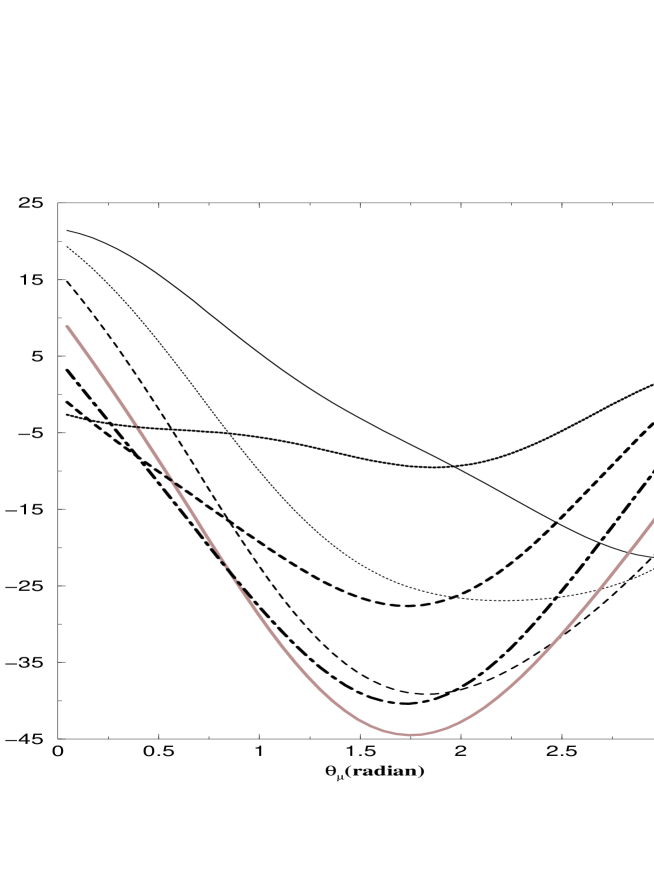
Figure 4: Plot of the b quark mass correction $\Delta m_{b}/m_{b}$ as a function of $\theta_{\mu}$ for various values of $\xi_{3}$. The other input parameters are: $m_{0}=m_{\frac{1}{2}}=200$ GeV, $\xi_{1}=.5$, $\xi_{2}=.659$, $\alpha_{A_{0}}=1.0$, $|A_{0}|=4$, and $\tan\beta=50$. The curves in descending order at the point $\theta_{\mu}=0$ correspond to $\xi_{3}=0,0.5,1.0,1.5,2.0,2.5,3.0$.

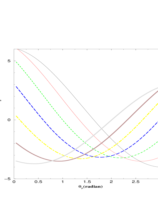
Figure 5: Plot of the b quark mass correction $\Delta m_{b}/m_{b}$ as a function of $\theta_{\mu}$.for various values of $\xi_{3}$. The other input parameters are: $m_{0}=m_{\frac{1}{2}}=200$ GeV, $\xi_{1}=.5$, $\xi_{2}=.659$, $\alpha_{A_{0}}=1.0$, $|A_{0}|=4$, and $\tan\beta=5$. The curves in descending order at the point $\theta_{\mu}=0.5$ correspond to $\xi_{3}=0,0.5,1.0,1.5,2.0,2.5,3.0$.

We begin with a discussion of the effects of CP phases on on the SUSY QCD and the SUSY electroweak correction to the b quark mass. In Fig. 3 a plot of the b quark mass correction as a function of $\theta_{\mu}$ is given for values of $\tan\beta$ ranging from 3 to 50. One finds that the correction is very sensitively dependent on $\theta_{\mu}$ as the value of $\theta_{\mu}$ affects both the sign and the magnitude of the correction. Thus the correction can vary from zero to as much as 30% in some regions of the parameter space and can also change its sign dependent on the value of $\theta_{\mu}$. In Fig. 4 a similar plot is given as a function of $\theta_{\mu}$ for different values of $\xi_{3}$ for the case $\tan\beta=50$. One finds that $\Delta m_{b}$ is also a very sensitive function of the phase $\xi_{3}$ and as in the case of $\theta_{\mu}$ this phase can also change both the magnitude as well as the sign of the b quark correction. In Fig. 5 we give a plot similar to that of Fig. 4 for the case of $\tan\beta=5$. The conclusions here are very similar to those for Fig. 4 except that the over all magnitude of the correction is typically smaller due to the smaller value of $\tan\beta$ in this case. In Fig. 6 a plot of the b quark correction as a function of $\alpha_{A_{0}}$ for various values of $|A_{0}|$ is given. One finds again a very strong dependence of the b quark correction on both $\alpha_{A_{0}}$ as well as on $|A_{0}|$. This strong dependence is less obvious than the dependence on $\theta_{\mu}$ and $\xi_{3}$ and arises from their effects on the stop and sbottom masses and via the dependence of the matrices that diagonalize the stop and sbottom mass matrices on $\alpha_{A_{0}}$ and on $|A_{0}|$. In Fig. 7 we give a plot of the b quark correction as a function of $\tan\beta$ for the three cases of Table 1 of Ref.[20] which satisfy the edm constraints for the electron, the neutron and for the $H_{g}$ atom for value of $\tan\beta=50$. The corresponding cases where the phases are all set to zero are also plotted. The plot shows that the effect of phases consistent with the edm constraints can produce large effects on the b quark mass.

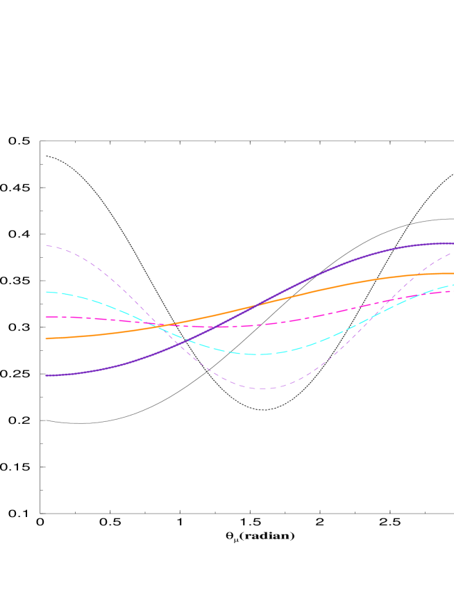
Figure 8: Plot of the top quark mass correction $\Delta m_{t}/m_{t}$ as a function of $\theta_{\mu}$ for values of $\tan\beta$ ranging from 3 to 50. The other input parameters are: $m_{0}=m_{\frac{1}{2}}=200$ GeV, $\xi_{1}=.5$, $\xi_{2}=.659$, $\xi_{3}=.633$, $\alpha_{A_{0}}=1.0$, and $|A_{0}|=4$. The curves in ascending order at the point $\theta_{\mu}=0$ correspond to $\tan\beta=3,5,10,20,30,40,50$.

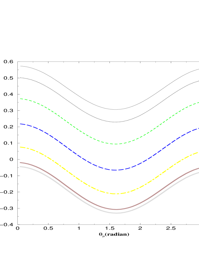
Figure 9: Plot of the top quark mass correction $\Delta m_{t}/m_{t}$ in percentage as a function of $\theta_{\mu}$ for various values of $\xi_{3}$. The other input parameters are: $m_{0}=m_{\frac{1}{2}}=200$ GeV, $\xi_{1}=.5$, $\xi_{2}=.659$, $\alpha_{A_{0}}=1.0$, $|A_{0}|=4$, and $\tan\beta=50$. The curves in descending order at the point $\theta_{\mu}=\pi$ correspond to $\xi_{3}=0,0.5,1.0,1.5,2.0,2.5,3.0$.

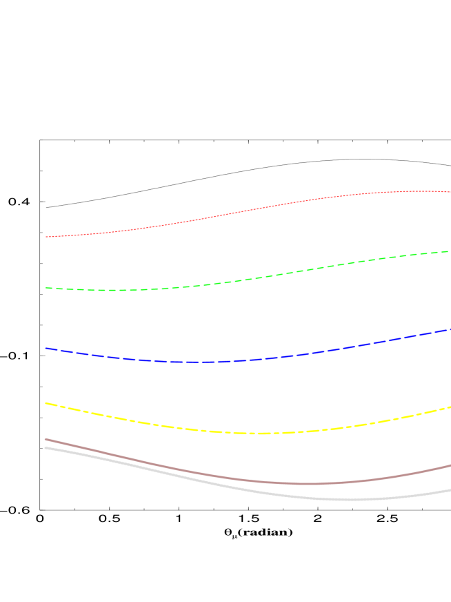
Figure 10: Plot of the top quark mass correction $\Delta m_{t}/m_{t}$ in percentage as a function of $\theta_{\mu}$ for various values of $\xi_{3}$. The other input parameters are: $m_{0}=m_{\frac{1}{2}}=200$ GeV, $\xi_{1}=.5$, $\xi_{2}=.659$, $\alpha_{A_{0}}=1.0$, $|A_{0}|=4$, and $\tan\beta=5$. The curves in descending order at the point $\theta_{\mu}=\pi$ correspond to $\xi_{3}=0,0.5,1.0,1.5,2.0,2.5,3.0$

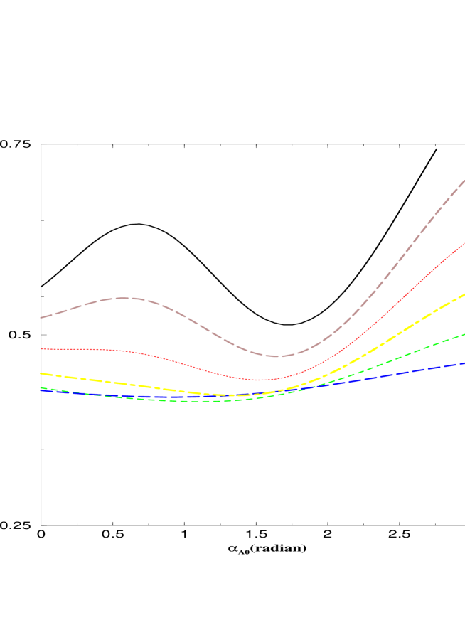
Figure 11: Plot of the top quark mass correction $\Delta m_{t}/m_{t}$ in percentage as a function of $\alpha_{A_{0}}$ for various values of $|A_{0}|$. The other input parameters are: $m_{0}=m_{\frac{1}{2}}=200$ GeV, $\xi_{1}=.5$, $\xi_{2}=.659$, $\xi_{3}=.633$, $\theta_{\mu}=\pi$ and $\tan\beta=50$. The curves in ascending order at the point $\alpha_{A_{0}}=2.5$ correspond to $|A_{0}|=1,2,3,4,5,6$

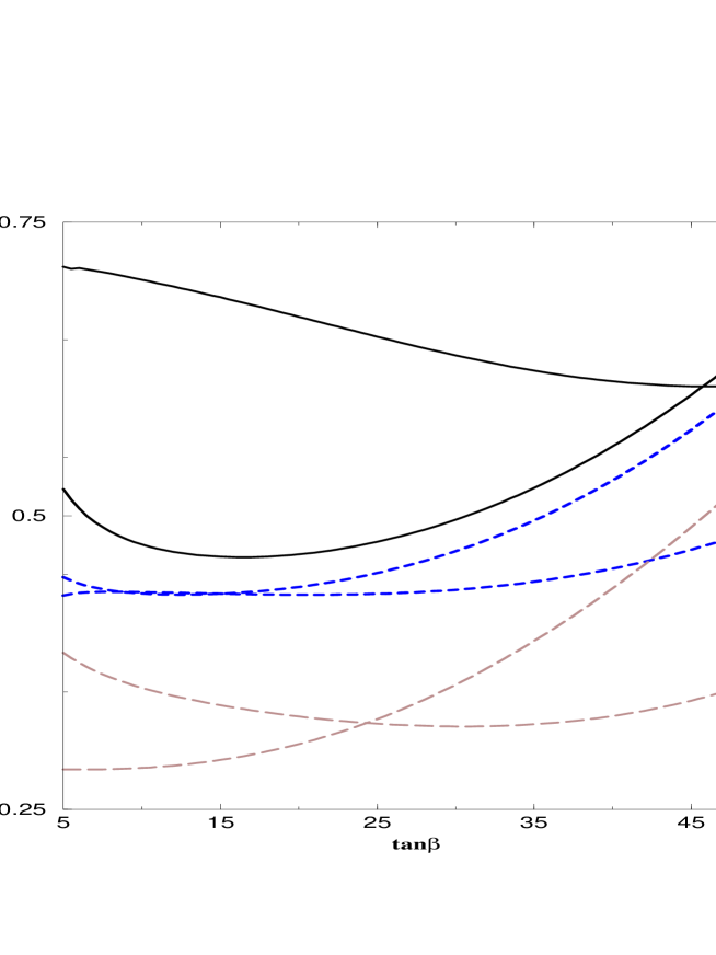
Figure 12: Plot of the top quark mass correction $\Delta m_{t}/m_{t}$ in percentage as a function of $\tan\beta$ for the three cases (a), (b) and (c) of Table 1 of Ref.[20] where the EDM constraints for the electron, the neutron and $H_{g}^{199}$ atom are satisfied for the case $\tan\beta=50$. The long dashed curve with intercept at $\tan\beta=50$ of 0.36 is for the case (a) where $m_{0}=m_{\frac{1}{2}}=200$ GeV, $A_{0}=4$, $\alpha_{A_{0}}=1$, $\xi_{1}=.5$, $\xi_{2}=.659$, $\xi_{3}=.633$. The solid curve with intercept at $\tan\beta=50$ of 0.61 is for the case (b) where $m_{0}=m_{\frac{1}{2}}=370$ GeV, $A_{0}=4$, $\alpha_{A_{0}}=2$, $\xi_{1}=.6$, $\xi_{2}=.653$, $\xi_{3}=.672$. The dashed curve with intercept at $\tan\beta=50$ of 0.49 is for the case (c) where $m_{0}=m_{\frac{1}{2}}=320$ GeV, $A_{0}=3$, $\alpha_{A_{0}}=.8$, $\xi_{1}=.4$, $\xi_{2}=.668$, $\xi_{3}=.6$. $\theta_{\mu}=2.5$ in all cases. The other three similar curves have all the same parameters as cases (a), (b), and (c) above except that phases are set to zero.

An analysis similar to the above for the correction to the top quark mass is given in figures Fig. 8, Fig. 9, Fig. 10, Fig. 11, and Fig. 12. Thus in Fig. 8 we give a plot of the top quark correction as a function of the $\theta_{\mu}$ for all the same parameters as in Fig. 3. As in the case of the b quark correction here also one finds that the correction to the top quark mass is very strongly dependent on $\theta_{\mu}$. However, unlike the case of the b quark correction the correction to the top quark mass is typically less than a percent which means that the SUSY loop correction to the top quark mass is likely to be at the level of a GeV or so. Such an effect could still be significant at the level of precision theoretical analyses. Very similar conclusions follow from the analysis of Fig. 9, Fig. 10, Fig. 11, and Fig. 12 which parallel the analysis of Fig. 4, Fig. 5, Fig. 6, and Fig. 7. As in the b quark correction here also one finds that the SUSY QCD and SUSY electroweak corrections to the top quark mass are strongly dependent on the phases $\xi_{3}$, $\alpha_{A_{0}}$ and on the parameters $m_{0}$, $m_{\frac{1}{2}}$ and $|A_{0}|$.

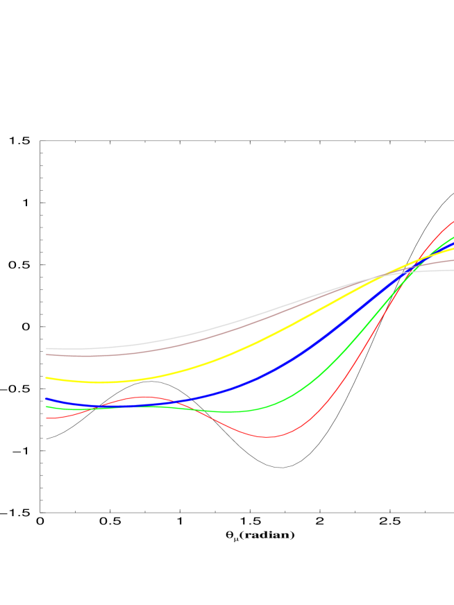
Figure 13: Plot of the tau lepton mass correction $\Delta m_{\tau}/m_{\tau}$ as a function of $\theta_{\mu}$ for values of $\tan\beta$ ranging from 3 to 50. The other input parameters are: $m_{0}=m_{\frac{1}{2}}=200$ GeV, $\xi_{1}=.5$, $\xi_{2}=.659$, $\xi_{3}=.633$, $\alpha_{A_{0}}=1.0$, and $|A_{0}|=4$. The curves in ascending order at the point $\theta_{\mu}=0$ correspond to $\tan\beta=50,40,30,20,10,5,3$.

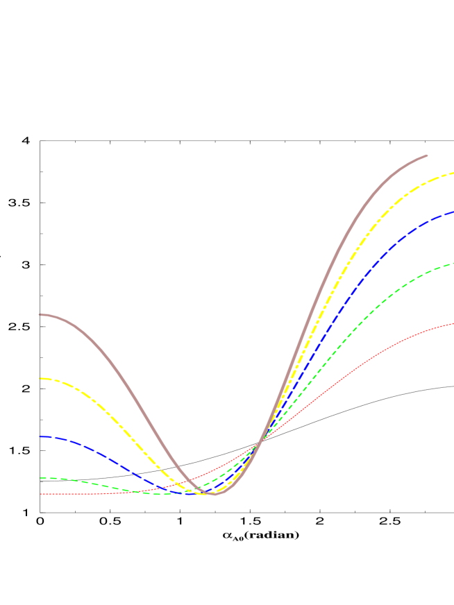
Figure 14: Plot of the tau lepton mass correction $\Delta m_{t}/m_{t}$ in percentage as a function of $\alpha_{A_{0}}$ for various values of $|A_{0}|$. The other input parameters are: $m_{0}=m_{\frac{1}{2}}=200$ GeV, $\xi_{1}=.5$, $\xi_{2}=.659$, $\xi_{3}=.633$, $\theta_{\mu}=\pi$ and $\tan\beta=50$. The curves in ascending order at the point $\alpha_{A_{0}}=2.5$ correspond to $|A_{0}|=1,2,3,4,5,6$

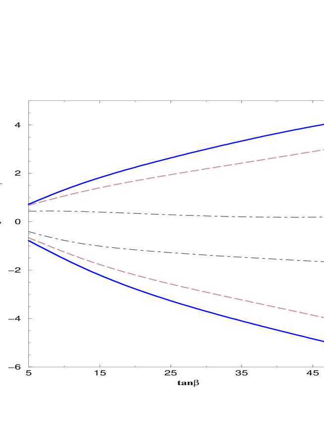
Figure 15: Plot of the tau lepton mass correction $\Delta m_{\tau}/m_{\tau}$ in percentage as a function of $\tan\beta$ for the three cases (a), (b) and (c) of Table 1 of Ref.[20] where the EDM constraints for the electron, the neutron and $H_{g}^{199}$ atom are satisfied for the case $\tan\beta=50$. The upper dot-dashed curve is for the case (a) where $m_{0}=m_{\frac{1}{2}}=200$ GeV, $A_{0}=4$, $\alpha_{A_{0}}=1$, $\xi_{1}=.5$, $\xi_{2}=.659$, $\xi_{3}=.633$. The upper solid curve is for the case (b) where $m_{0}=m_{\frac{1}{2}}=370$ GeV, $A_{0}=4$, $\alpha_{A_{0}}=2$, $\xi_{1}=.6$, $\xi_{2}=.653$, $\xi_{3}=.672$. The upper long dashed curve is for the case (c) where $m_{0}=m_{\frac{1}{2}}=320$ GeV, $A_{0}=3$, $\alpha_{A_{0}}=.8$, $\xi_{1}=.4$, $\xi_{2}=.668$, $\xi_{3}=.6$. $\theta_{\mu}=2.5$ in all cases. The lower three similar curves have all the same parameters as cases (a), (b), and (c) above except that phases are set to zero.

Finally, we discuss the numerical size of the correction to the $\tau$ lepton mass. In Fig. 13 we give a plot of the correction to the $\tau$ lepton mass as a function of $\theta_{\mu}$ for all the same parameters as in Fig. 3 and in Fig. 8. As in the case of the correction to the b quark mass and to the top quark mass here also one finds that the correction to the $\tau$ lepton mass is very strongly dependent on $\theta_{\mu}$. However, the numerical size of the correction is significantly smaller than the correction to the b quark mass although generally bigger percentage wise than the percentage correction to the top quark mass. Again such effects could be relevant in precision physics. In Fig. 14, analogous to the case of Fig. 6 for the b quark and Fig. 11 for the case of the top quark, a plot of the $\tau$ lepton correction as a function of $\alpha_{A_{0}}$ for various values of $|A_{0}|$ is given. As in the case of Fig. 6 and Fig. 11 one finds a very strong dependence of the $\tau$ lepton mass correction on $\alpha_{A_{0}}$ and on $|A_{0}|$. In Fig. 15, as in the case of Fig. 7 for the b quark mass and in the case of Fig. 12 for the top quark mass, we give a plot of the $\tau$ lepton correction as a function of $\tan\beta$ for the three cases of Table 1 of Ref.[20] which satisfy the edm constraints for the electron, the neutron and for the $H_{g}$ atom for value of $\tan\beta=50$. The corresponding cases where the phases are all set to zero are also plotted. The plot shows that the effect of phases consistent with the EDM constraints can produce large effects on the $\tau$ lepton mass. Fig. 15 shows that the loop correction to the $\tau$ lepton mass can become as large as 5%. Thus overall we find that consistently in all cases considered the supersymmetric QCD effects and the supersymmetric electroweak effects are strongly dependent on CP phases. They can change both the sign as well as the magnitude of the one loop correction. Such effects will have important implications on low energy phenomena where supersymmetry QCD and supersymmetric electroweak effects enter. An example of this is the analysis of branching ratio for the decay $B^{0}_{s,d}\rightarrow l^{+}l^{-}$ decay which is strongly affected by the SUSY QCD corrections[20, 33] and is also very sensitive to the CP phases. As pointed out in Sec.1, Yukawa coupling unification is sensitive to SUSY QCD and SUSY electroweak loop correction and thus will also be sensitive to the CP phases.

6 Conclusion

In this paper we have computed the effects of CP phases on the $b$ and $t$ quark masses and the $\tau$ lepton mass. In Sec.2 we discussed the general technique for the computation of QCD and electroweak loop corrections to the fermion masses and specifically analysed the contributions to the b quark mass arising from the gluino, chargino and neutralino exchange contributions. We also checked that our results agree with previous analyses in the limit when phases are all set to zero and $\tan\beta$ is taken to be large. In Sec.3 we extended the analysis to compute corrections to the top quark mass arising from the gluino, chargino and neutralino exchange contributions. In Sec.4 we extended the analysis to compute the SUSY electroweak corrections to the $\tau$ lepton mass arising from chargino and neutralino exchange contributions. These analyses were carried out allowing for the most general allowed set of CP phases and without a constraint on $\tan\beta$. Thus the analysis presented in this paper is valid not only for large $\tan\beta$ but also for moderate and small values of $\tan\beta$. The analysis presented in Secs.2, 3 and 4 is the first complete one loop result of the corrections to the b and t quark masses and to the $\tau$ lepton mass allowing for all allowed phases and valid for all $\tan\beta$. In Sec.5 we gave an exhaustive numerical analysis of the size of the SUSY QCD and SUSY electroweak corrections to the b and t quark masses and to the $\tau$ lepton mass. One finds that the numerical size of the corrections to the b quark mass can be as large as 30% while the correction to the $\tau$ lepton mass as large as 5%. However, we find that the correction is typically less than a 1% for the case of the top quark mass. Further, in all cases analyzed one finds that the correction is sharply dependent on the CP phases. Thus one finds that both the magnitude as well as the sign may be affected by the presence of the CP phases. The loop corrections are of great importance in unified models specifically those involving Yukawa coupling unification, e.g., $b-\tau$ unification for SU(5) and $b-t-\tau$ unification for a class of SO(10) models. More generally these loop corrections will be of import in the study of quark-lepton textures in the presence of CP phases. The SUSY QCD and SUSY electroweak corrections to the b quark mass is also of great importance in the analysis of low energy phenomena where the b quark mass enters prominently such as phenomena involving B mesons. Thus, for example, the decay $B^{0}_{s,d}\rightarrow l^{+}l^{-}$ is strongly affected by the SUSY QCD and SUSY electroweak corrections[20, 33] .

Acknowledgments
This research was supported in part by NSF grant PHY-0139967.

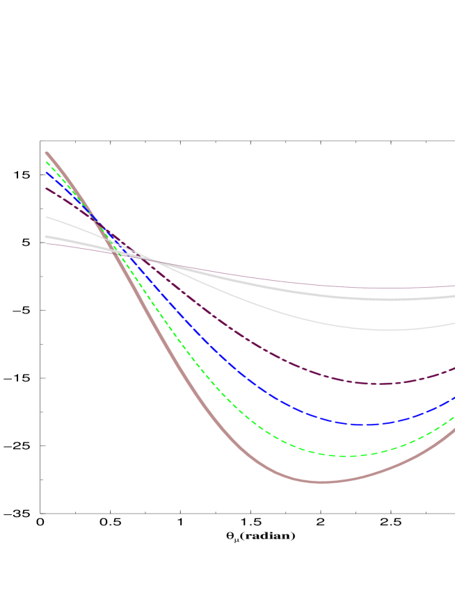
Figure 3: Plot of the b quark mass correction $\Delta m_{b}/m_{b}$ as a function of $\theta_{\mu}$ The curves in descending order at the point $\theta_{\mu}=\pi$ correspond to $\tan\beta=3,5,10,20,30,40,50$. The other input parameters are: $m_{0}=m_{\frac{1}{2}}=200$ GeV, $\xi_{1}=.5$, $\xi_{2}=.659$, $\xi_{3}=.633$, $\alpha_{A_{0}}=1.0$, and $|A_{0}|=4$. All angles here and in succeeding figure captions are in radians.

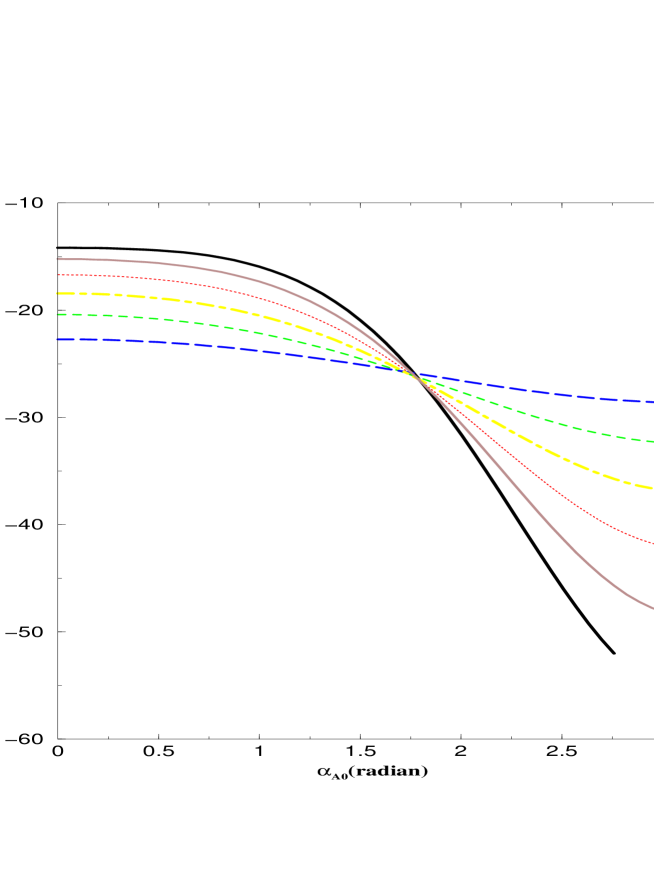
Figure 6: Plot of the b quark mass correction $\Delta m_{b}/m_{b}$ as a function of $\alpha_{A_{0}}$ for various values of $|A_{0}|$. The other input parameters are: $m_{0}=m_{\frac{1}{2}}=200$ GeV, $\xi_{1}=.5$, $\xi_{2}=.659$, $\xi_{3}=.633$, $\theta_{\mu}=\pi/4$, and $\tan\beta=50$. The curves in descending order at the point $\alpha_{A_{0}}=2.5$ correspond to $|A_{0}|=1,2,3,4,5,6$.

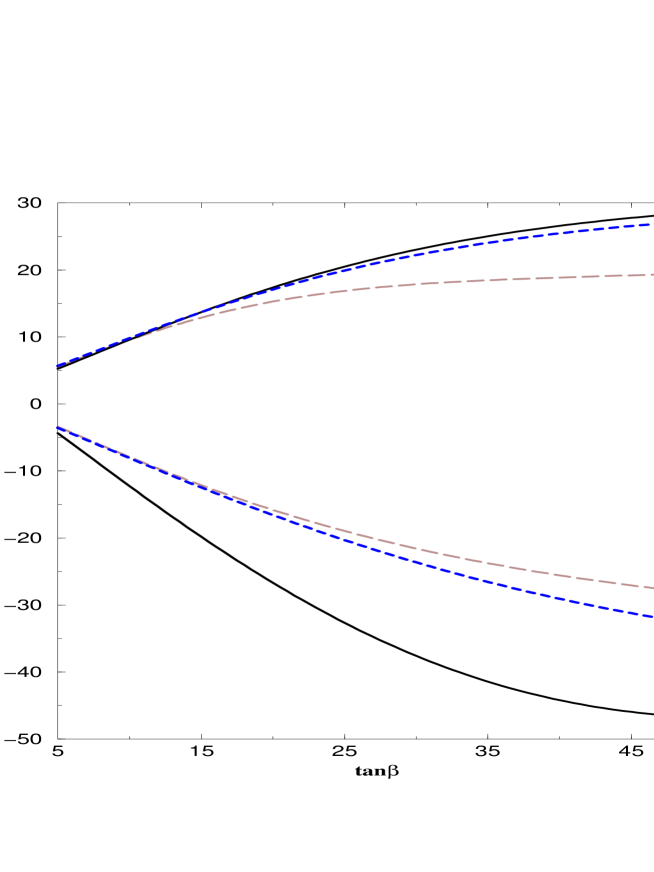
Figure 7: Plot of the b quark mass correction $\Delta m_{b}/m_{b}$ as a function of $\tan\beta$ for the three cases (a), (b) and (c) of Table 1 of Ref.[20] where the EDM constraints for the electron, the neutron and $H_{g}^{199}$ atom are satisfied for the case $\tan\beta=50$. Among the curves in the lower half plane corresponding to negative correction to the b quark mass, the long dashed curve corresponds to the case (a) where $m_{0}=m_{\frac{1}{2}}=200$ GeV, $A_{0}=4$, $\alpha_{A_{0}}=1$, $\xi_{1}=.5$, $\xi_{2}=.659$, $\xi_{3}=.633$; the solid curve corresponds to the case (b) where $m_{0}=m_{\frac{1}{2}}=370$ GeV, $A_{0}=4$, $\alpha_{A_{0}}=2$, $\xi_{1}=.6$, $\xi_{2}=.653$, $\xi_{3}=.672$; the dashed curve corresponds to the case (c) where $m_{0}=m_{\frac{1}{2}}=320$ GeV, $A_{0}=3$, $\alpha_{A_{0}}=.8$, $\xi_{1}=.4$, $\xi_{2}=.668$, $\xi_{3}=.6$. $\theta_{\mu}=2.5$ in all cases. The three similar curves in the upper half plane are for the three cases above when the phases are all set to zero.

References

• [1] H. Arason, D.J. Castano, B.E. Kesthelyi, S. Mikaelian, E.J. Piard, P. Ramond, and B.D. Wright, Phys. Rev. Lett. 67, 2933(1991); V. Barger, M.S. Berger, and P. Ohman, Phys. Lett. B314, 351(1993); Phys. Rev. D47, 1093(1993); T. Dasgupta, P. Mamales and P. Nath, Phys. Rev. D52, 5366(1995); D. Pierce, J. Bagger, K. Matchev and R. Zhang, Nucl. Phys. B491, 3(1997); H. Baer, H. Diaz, J. Ferrandis and X. Tata, Phys. Rev. D61, 111701(2000); W. de Boer, M. Huber, A.V. Gladyshev, D.I. Kazakov, Eur.Β Phys.Β J.Β C 20, 689 (2001).
• [2] T.Β Banks, Nucl.Β Phys.Β B 303, 172 (1988); M.Β Olechowski and S.Β Pokorski, Phys.Β Lett.Β B 214, 393 (1988); S.Β Pokorski, Nucl.Β Phys. (Proc. Suppl.) B13, 606 (1990); B.Β Ananthanarayan, G.Β Lazarides and Q.Β Shafi, Phys.Β Rev.Β D 44, 1613 (1991) S.Β Dimopoulos, L.Β J.Β Hall and S.Β Raby, Phys.Β Rev.Β Lett.Β  68, 1984 (1992).
• [3] H. Baer and J. Ferrandis, Phys. Rev. Lett.87, 211803 (2001); T.Β Blazek, R.Β Dermisek and S.Β Raby, Phys.Β Rev.Β Lett.Β  88, 111804 (2002); Phys.Β Rev.Β D 65, 115004 (2002); S.Β Komine and M.Β Yamaguchi, Phys.Β Rev.Β D 65, 075013 (2002); U.Β Chattopadhyay and P.Β Nath, Phys.Β Rev.Β D 65, 075009 (2002); M.Β E.Β Gomez, G.Β Lazarides and C.Β Pallis, Nucl.Β Phys.Β B 638, 165 (2002); B.Β Bajc, G.Β Senjanovic and F.Β Vissani, [hep-ph/0210207]; J.Β Ferrandis, [hep-ph/0211370]; K.Β Tobe and J.Β D.Β Wells, arXiv:hep-ph/0301015.
• [4] L.Β J.Β Hall, R.Β Rattazzi and U.Β Sarid, Phys.Β Rev.Β D 50, 7048 (1994).
• [5] M.Β Carena, M.Β Olechowski, S.Β Pokorski and C.Β E.Β Wagner, Nucl.Β Phys.Β B 426, 269 (1994).
• [6] D.Β M.Β Pierce, J.Β A.Β Bagger, K.Β T.Β Matchev and R.Β j.Β Zhang, Nucl.Β Phys.Β B 491, 3 (1997).
• [7] M.Β Carena, D.Β Garcia, U.Β Nierste and C.Β E.Β Wagner, Nucl.Β Phys.Β B 577, 88 (2000) [arXiv:hep-ph/9912516].
• [8] M.Β Carena and H.Β E.Β Haber, arXiv:hep-ph/0208209;
• [9] A.H. Chamseddine, R. Arnowitt and P. Nath, Phys. Rev. Lett. 49, 970 (1982); Β R. Barbieri, S. Ferrara and C.A. Savoy, Phys. Lett. B 119, 343 (1982); Β L. Hall, J. Lykken, and S. Weinberg, Phys. Rev. D 27, 2359 (1983):Β  P. Nath, R. Arnowitt and A.H. Chamseddine, Nucl. Phys. B 227, 121 (1983).
• [10] E. Commins, et. al., Phys. Rev. A50, 2960(1994).
• [11] P.G. Harris et.al., Phys. Rev. Lett. 82, 904(1999).
• [12] S.Β K.Β Lamoreaux, J.Β P.Β Jacobs, B.Β R.Β Heckel, F.Β J.Β Raab and E.Β N.Β Fortson, Phys.Β Rev.Β Lett.Β  57, 3125 (1986).
• [13] See, e.g., J. Ellis, S. Ferrara and D.V. Nanopoulos, Phys. Lett. B114, 231(1982); W. Buchmuller and D. Wyler, Phys. Lett. B121,321(1983); M. Dugan, B. Grinstein and L. Hall, Nucl. Phys. B255, 413(1985); R.Garisto and J. Wells, Phys. Rev. D55, 611(1997).
• [14] P. Nath, Phys. Rev. Lett.66, 2565(1991); Y. Kizukuri and N. Oshimo, Phys.Rev.D46,3025(1992).
• [15] K.S. Babu, B. Dutta and R. N. Mohapatra, Phys. Rev. D61, 091701(2000).
• [16] T. Ibrahim and P. Nath, Phys.Β Lett.Β B 418, 98 (1998); Phys. Rev. D57, 478(1998); T. Falk and K Olive, Phys. Lett. B 439, 71(1998); M. Brhlik, G.J. Good, and G.L. Kane, Phys. Rev. D59, 115004 (1999); A. Bartl, T. Gajdosik, W. Porod, P. Stockinger, and H. Stremnitzer, Phys. Rev. 60, 073003(1999); S. Pokorski, J. Rosiek and C.A. Savoy, Nucl.Phys. B570, 81(2000); E.Β Accomando, R.Β Arnowitt and B.Β Dutta, Phys.Β Rev.Β D 61, 115003 (2000); U. Chattopadhyay, T. Ibrahim, D.P. Roy, Phys.Rev.D64:013004,2001; C.Β S.Β Huang and W.Β Liao, Phys.Β Rev.Β D 61, 116002 (2000); ibid, Phys.Β Rev.Β D 62, 016008 (2000); A.Bartl, T. Gajdosik, E.Lunghi, A. Masiero, W. Porod, H. Stremnitzer and O. Vives, hep-ph/0103324. For analyses in the context string and brane models see, M. Brhlik, L. Everett, G. Kane and J. Lykken, Phys. Rev. Lett. 83, 2124, 1999; Phys. Rev. D62, 035005(2000); E. Accomando, R. Arnowitt and B. Datta, Phys. Rev. D61, 075010(2000); T. Ibrahim and P. Nath, Phys. Rev. D61, 093004(2000).
• [17] D. Chang, W-Y.Keung,and A. Pilaftsis, Phys. Rev. Lett. 82, 900(1999).
• [18] T.Β Ibrahim and P.Β Nath, Phys.Β Rev.Β D 61, 093004 (2000) [arXiv:hep-ph/9910553].
• [19] T. Falk, K.A. Olive, M. Prospelov, and R. Roiban, Nucl. Phys. B560, 3(1999); V.Β D.Β Barger, T.Β Falk, T.Β Han, J.Β Jiang, T.Β Li and T.Β Plehn, Phys.Β Rev.Β D 64, 056007 (2001); S.Abel, S. Khalil, O.Lebedev, Phys. Rev. Lett. 86, 5850(2001)
• [20] T.Β Ibrahim and P.Β Nath, Phys.Β Rev.Β D 67, 016005 (2003)
• [21] A. Pilaftsis, Phys. Rev. D58, 096010; Phys. Lett.B435, 88(1998); Β A. Pilaftsis and C.E.M. Wagner, Nucl. Phys. B553, 3(1999); Β D.A. Demir, Phys. Rev. D60, 055006(1999); Β S.Β Y.Β Choi, M.Β Drees and J.Β S.Β Lee, Phys.Β Lett.Β B 481, 57 (2000); Β M.Β Boz, Mod.Β Phys.Β Lett.Β A 17, 215 (2002).
• [22] T. Ibrahim and P. Nath, Phys.Rev.D63:035009,2001; hep-ph/0008237; T.Β Ibrahim, Phys.Β Rev.Β D 64, 035009 (2001); T.Β Ibrahim and P.Β Nath, Phys.Β Rev.Β D 66, 015005 (2002); Β S.Β W.Β Ham, S.Β K.Β Oh, E.Β J.Β Yoo, C.Β M.Β Kim and D.Β Son, arXiv:hep-ph/0205244.
• [23] M.Β Carena, J.Β R.Β Ellis, A.Β Pilaftsis and C.Β E.Β Wagner, Nucl.Β Phys.Β B 625, 345 (2002) [arXiv:hep-ph/0111245]. ; M.Β Carena, J.Β Ellis, S.Β Mrenna, A.Β Pilaftsis and C.Β E.Β Wagner, arXiv:hep-ph/0211467.
• [24] S.Β Mrenna, G.Β L.Β Kane and L.Β T.Β Wang, Phys.Β Lett.Β B 483, 175 (2000); A. Dedes, S. Moretti, Phys.Rev.Lett.84:22-25,2000; Nucl.Phys.B576:29-55,2000; S.Y.Choi and J.S. Lee, Phys. Rev.D61, 111702(2000).
• [25] V. Barger, Tao Han, Tian-Jun Li, Tilman Plehn, Phys.Lett.B475:342-350,2000.
• [26] S.Β Y.Β Choi, M.Β Guchait, J.Β Kalinowski and P.Β M.Β Zerwas, Phys.Β Lett.Β B 479, 235 (2000); Β S.Β Y.Β Choi, A.Β Djouadi, H.Β K.Β Dreiner, J.Β Kalinowski and P.Β M.Β Zerwas, Eur.Β Phys.Β J.Β C 7, 123 (1999).
• [27] T.Β Ibrahim and P.Β Nath, Phys.Β Rev.Β D 62, 015004 (2000) ; Phys.Β Rev.Β D 61, 095008 (2000).
• [28] C.Β S.Β Huang and W.Β Liao, Phys.Β Lett.Β B 538, 301 (2002).
• [29] See, e.g., A.Β Masiero and H.Β Murayama, Phys.Β Rev.Β Lett.Β  83, 907 (1999); Β S.Β Khalil and T.Β Kobayashi, Phys.Β Lett.Β B 460, 341 (1999); Β D.Β A.Β Demir, A.Β Masiero and O.Β Vives, Phys.Β Lett.Β B 479, 230 (2000).
• [30] T.Β Ibrahim and P.Β Nath, arXiv:hep-ph/0210251; arXiv:hep-ph/0207213.
• [31] J.Β F.Β Gunion and H.Β E.Β Haber, Nucl.Β Phys.Β B 272, 1 (1986) [Erratum-ibid.Β B 402, 567 (1993)].
• [32] T.Β Ibrahim and P.Β Nath, Phys.Β Rev.Β D 58, 111301 (1998).
• [33] J.Β K.Β Mizukoshi, X.Β Tata and Y.Β Wang, Phys.Β Rev.Β D 66, 115003 (2002).
Refer to caption