The Bohr Atom of Glueballs

Recently Buniy and Kephart[1] made an astonishing empirical observation, which anyone can reproduce at home. Measure the lengths of closed knots tied from ordinary rope. The “double do-nut”, and the beautiful trefoil knot (Fig. 1) are examples. Tie the knots tightly, and glue or splice the tails into a seamless unity. Compare two knots with corresponding members of the mysterious particle states known as “glueball” candidates in the literature[2]. Propose that the microscopic glueball mass ought to be proportional to the macroscopic mass of the corresponding knot. Fit two parameters, then predict 12 of 12 remaining glueball masses with extraordinary accuracy, knot by knot. Here we relate these observations to the fundamental gauge theory of gluons, by recognizing a hidden gauge symmetry bent into the knots. As a result the existence and importance of a gluon mass parameter is clarified. Paradoxically forbidden by the usual framework[3], the gluon mass cannot be expressed in the usual coordinates, but has a natural meaning in the geometry of knots.

The Buniy-Kephart (BK) discovery is dramatic and can be called the “Bohr atom” of glueballs. Bohr’s quantization[4] is explained by a whole number of vibrations of an electronic wave function traversing a closed orbit. The BK explanation postulates a “solitonic” magnetic flux rope of gauge fields, traversing a closed but knotted path with a whole number of self- crossings. The energy, and then the mass of the flux rope is proportional to the length of the rope. The glueball mass spectrum follows[1].

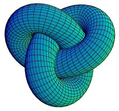
Figure 1: A tightly wrapped trefoil knot, identified as the second member of the glueball spectrum.

Deep questions of consistency hide in this picture. The fundamental theory of glue[3], Quantum Chromodynamics (QCD), predicts glueballs[5] only indirectly, through the existence of certain singlet operators. Decades have passed seeking a clear signature[5]. The QCD static energy density has a term going like $\frac{1}{2}\vec{B}^{2}$, the magnetic energy density. Ordinary magnetic flux (the field lines of “bar-magnets”) flows in closed loops, yet strict flux conservation is not a general property of the more elaborate chomo-flux of QCD[3]. The hopeful logic holds that if a flux is conserved and arranged into a constant width tube, then the classical energy and glueball mass goes like the length of the knot. So far so good: yet the theory has no solitons! QCD and other gauge theories lack a mass scale upon which to base any particular soliton mass. The quantum treatment inducing a scale called $\Lambda_{QCD}$ does not change this. Moreover, the requirements of a gauge theory are exacting. It is commonly held impossible to add a mass scale affecting the infrared (large-scale) structure, and retain gauge invariance, the raison d’$\hat{e}$tre of glue itself.

The culprit is confinement, the phenomenon that gauge fields and quarks cannot get outside of the strongly interacting particles. Confinement is poorly understood. “Effective” theories are proposed as surrogates for the fundamental one. Fadeev and Niemi[6] constructed knotted solitons, such as the trefoil[7] (Fig. 1), in an ad-hoc effective theory. Yet the picture of conserved flux and knotted rope is a hybrid. There has been no direct connection between solitons, knots, and any underlying gauge fields which form the fundamental glue.

Look afresh at the effective theory making knots. The basic variable is a real-valued 3-component unit vector field $\hat{n}(\vec{x})$. The Lagrangian density is

$$L = \frac{m^{2}}{4}\partial_{\mu}\hat{n}\cdot\partial^{\mu}\hat{n}-\frac{1}{g^{2}}(\hat{n}\cdot\partial_{\mu}\hat{n}\times\partial_{\nu}\hat{n})(\hat{n}\cdot\partial^{\mu}\hat{n}\times\partial^{\nu}\hat{n})$$ (1)

$$= m^{2}L_{2}+\frac{1}{g^{2}}L_{4}.$$

Here $\partial_{\mu}=\partial/\partial x^{\mu}$, while $\cdot$ and $\times$ denote the dot and cross product of three dimensional space. No flux tubes are obvious in Eq. 1. Nor are local transformations of $\hat{n}(x)$ a symmetry. Therefore if the theory is related to a gauge theory, we propose it is the invariant coordinatization of a gauge theory.

An invariant formulation is possible by embedding gauge-theory geometry in a larger space. Interpret $\hat{n}(x)$ as a vector perpendicular to a 2-surface, spanned by a local tangent frame $\hat{e}^{a}$, $a=1,\,2$, $\hat{e}^{a}\cdot\hat{e}^{b}=\delta^{ab}$. Transfer attention to the surface. Its bending and stretching fixes the system’s energy. Surface coordinates are related non-invertibly by

$$\hat{n}=\hat{e}^{1}\times\hat{e}^{2}.$$

Compare the freedoms of the $\hat{n},\,\hat{e}$ descriptions: use of the tangent-frame “inner” $\hat{e}$’s involves one extra angle $\phi(x)$. This angle parametrizes the orientation of the frame on the surface. Angle $\phi(x)$.is not determined by the Lagrange density depending on $\hat{n}(x)$ and can be freely chosen as an arbitrary smooth function of $\vec{x}$. There is a local symmetry

$$\left(\begin{array}[]{c }\hat{e}^{1}(x)\\ \hat{e}^{1}(x)\end{array}\right) \rightarrow R(x)\left(\begin{array}[]{c }\hat{e}^{1}(x)\\ \hat{e}^{1}(x)\end{array}\right)=\left(\begin{array}[]{cc }cos\phi(x)&sin\phi(x)\\ -sin\phi(x)&cos\phi(x)\end{array}\right)\left(\begin{array}[]{c }\hat{e}^{1}(x)\\ \hat{e}^{1}(x)\end{array}\right);$$ (10)

$$\hat{n}(x) \rightarrow \hat{n}(x).$$ (11)

Due to local invariance of $\hat{n}$, the system dynamics has a local $S0(2)$ gauge symmetry when expressed via the $e$’s. This happens to be just the same symmetry upon which flux tubes are based.

Let us explore the meaning of the separate terms. Some algebra yields

$$\hat{n}\cdot\partial_{\mu}\hat{n}\times\partial_{\nu}\hat{n}=-\frac{1}{2}(\,\partial_{\mu}\hat{e}_{k}^{1}\partial_{\nu}\hat{e}_{k}^{2}-\partial_{\nu}\hat{e}_{k}^{1}\partial_{\mu}\hat{e}_{k}^{2}\,).$$ (12)

A famous theorem says that invariants of local transformations must be a function of gauge-covariant derivatives[8]. Differential geometry defines a connection $A_{\mu}=\frac{1}{g}\hat{e}_{k}^{1}\partial_{\mu}\hat{e}^{2}$ to be used. Under Eq. 11 we have

$$A_{\mu}\rightarrow A_{\mu}^{\prime}(R(x)e)=A_{\mu}(e(x))+\partial_{\mu}\phi(x),$$ (13)

following by definition, and $A_{\mu}$ serves as a gauge field. Very nicely,

$$\frac{1}{g}\hat{n}\cdot\partial_{\mu}\hat{n}\times\partial_{\nu}\hat{n} = -\frac{1}{2}(\,\partial_{\mu}A_{\nu}-\partial_{\nu}A_{\mu}\,),$$ (14)

$$\equiv -\frac{1}{2}F_{\mu\nu};$$

$$\frac{1}{g^{2}}L_{4} = -\frac{1}{4}F_{\mu\nu}F^{\mu\nu}.$$ (15)

We find that $L_{4}$ actually is the usual Lagrangian of a hidden gauge theory! Flux conservation is established, defining $B_{i}=\frac{1}{2}\epsilon_{ijk}F_{jk}$, with $\vec{\nabla}\cdot\vec{B}=0$, a Bianchi identity, being the ancient law that “you can’t break a magnetic rope”.

What is the meaning of the $L_{2}$ term? Algebra gives

$$\frac{m^{2}}{4}\partial_{\mu}\hat{n}\cdot\partial^{\mu}\hat{n}=-\frac{m^{2}}{2}(A_{\mu}A^{\mu}-\frac{1}{2}\partial_{\mu}\hat{e}_{k}^{a}\partial_{\mu}\hat{e}_{k}^{a});$$

$$L=-\frac{1}{4}F_{\mu\nu}F^{\mu\nu}-\frac{1}{2}m^{2}A_{\mu}A^{\mu}+\frac{1}{4}m^{2}\partial_{\mu}\hat{e}_{k}^{a}\partial_{\mu}\hat{e}_{k}^{a}.$$ (16)

Geometry proves it is impossible to express $L$ entirely as a local function of $A_{\mu}.$ The geometrical meaning of $L_{2}$ is the sum of the squares of the principal curvatures of the bent and stretched 2-surface. The extrinsic (“bending”) curvatures depend on the embedding of the 2-surface in a higher space. In contrast, only intrinsic curvatures independent of embedding are expressed by $A$.

Dynamically, parameter $m$ defines an effective gluon mass. Addition of $(\partial_{\mu}e)^{2}$ terms gives Eq. 16 a different mass from the usual, non-gauge-invariant kind. Recall that varying $L_{4}$ with respect to $A$ would give the Yang-Mills (Maxwell) equations in the usual gauge theory. Instead vary the action with respect to frames $\hat{e}^{a}$, which after fixing the gauge, are just the same as varying with respect to $\hat{n}$. There are extra solutions because the bending of the knot has real physical energy in all forms of the knot’s curvature.

Does the same pattern extend to the non-Abelian theory? The answer is yes. Make incomplete frames $e_{K}^{a}$ on $K=1\ldots K_{max}$ complex dimensions. For a unitary group the frames are orthonormal, $e_{K}^{a}\bar{e}_{K}^{b}=\delta^{ab},\,a,\,b=1\ldots N.$ Let the frames transform as fundamental representations of a local group $U(x)$, $e_{K}^{a}\rightarrow U^{ab}(x)e_{K}^{b}$. The induced gauge field is $A^{ab}_{\mu}=-\frac{i}{g}e_{K}^{a}\partial_{\mu}\bar{e}_{K}^{b},$ with bar denoting the complex conjugate and $g$ the coupling constant. The gauge field transforms as $A(e,\,\bar{e};\,x)\rightarrow A(Ue,\,\bar{e}U^{-1};\,x)=U(x)A(x)U^{-1}(x)-\frac{i}{g}U(x)\partial U^{-1}(x),$ with indices suppressed. To allow field strength $F_{\mu\nu}^{ab}\neq 0$, the frames must be embedded in a space of dimension larger than the one they span: $K_{max}>N$. The formula for $m^{2}L_{2}=-\frac{m^{2}}{2}tr(A^{2}-\partial e\partial\bar{e})$, using “bar” for complex conjugation and $tr$ for trace over the indices, is unique and describes the lowest-order invariant.

Now ask again: How can it be posible that the modified gauge theory, with its gauge invariance and conserved magnetic flux, might have soliton masses proportional to the knot-lengths? The energy density from Eq. 16 consists of two terms, $m^{2}h_{2}$ and $\frac{1}{g^{2}}h_{4}$ with 2 and 4 derivatives, respectively. Suppose we find a static solution $\hat{n}(\vec{x})$. Compare its energy $E$ with the energy $E(\lambda)$ of a re-scaled configuration $\hat{n}_{\lambda}(\vec{x})=\hat{n}(\lambda\vec{x})$. Change variables to integrate over $\vec{x}_{\lambda}=\lambda\vec{x}$. This gives

$$E(\lambda)=\int\frac{d^{3}x_{\lambda}}{\lambda^{3}}\,\lambda^{2}m^{2}h_{2}(\hat{n}_{\lambda}(x_{\lambda}))+\frac{1}{g^{2}}\lambda^{4}h_{4}(\hat{n}_{\lambda}(x_{\lambda})).$$ (17)

The energy $E(\lambda)$ is stationary for all variations. Varying $\lambda$ at $\lambda=1$ must be stationary. This yields

$$\int d^{3}x\,m^{2}h_{2}(\lambda=1) = \int d^{3}x\,\frac{1}{g^{2}}h_{4}(\lambda=1)\equiv E_{4};$$

$$\>\>\>\>thus\>\>E(\lambda=1) = 2E_{4}$$

Using Eqs. 14, 15 the energy $E_{4}$ is the magnetic energy density cited earlier. The knotted soliton mass

$$M_{knot}=\frac{2}{2}\int d^{3}x\,\vec{B}^{2},$$ (18)

and the knotted soliton mass is proportional to the knot volume, just as proposed by BK. To complete the chain of logic, knot-volumes must go like the lengths of knots, implying constant rope width. This was already shown[6], although not yet shown for all knots. Industrially making higher order soliton knots is itself mind-bogglng in terms of variable $\hat{n}$. We suggest a procedure: First bend a solenoid along the knot. Solve a trial $\vec{A}$ with the right topology. Settle into the appropriate soliton by using a numerical relaxation method.

The theory of Eq. 16 is superbly suited to the phenomenological observations of Ref. [1]. To reiterate this conclusion, the data for the masses of the glueballs is inverted to find the gluon mass value. This restates observations in Ref. [1], and is not an independent test. Soliton masses scale like $m$, the gluon mass parameter, as the sole scale. For each glueball candidate mass $M_{j}$ we then calculate $m_{j}$, a trial mass parameter. The relation is

$$m(j)=\frac{M_{j}-\Delta M}{\beta L(j)}.$$ (19)

Here $\Delta M$ is a free parameter, hopefully small, representing quantum corrections. Take $L(j)$ from knot theory, made dimensionful with parameter $\beta$, which absorbs $g^{2}$ and the knot width-to-length ratio. The idea fails if the $m(J)$ take many different values. But the mass parameters $m(j)$ (Fig. 2) are found remarkably constant. One universal gluon mass: $m(j)\rightarrow m=$298 $\pm$ 19 MeV, $\Delta M=15.0\pm$84 MeV is supported by the fit. Parameter $\beta$ is not determined, and was adjusted so that the gluon mass is half the double-donut mass.

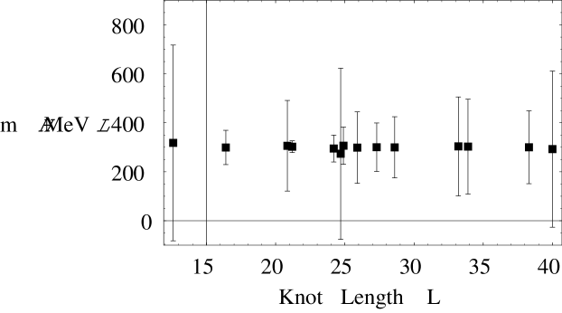
Figure 2: Gluon mass fitting parameters $m(j)=\frac{M_{j}-\Delta M}{\beta L(j)},$ as a function of knot length $L(j)$. Deduced mass values $m_{j}$ are nearly constant (dashed line $m=298$ MeV), indicating one universal mass parameter $m$ fits the data. The overall scale from $\beta$ is arbitrary. Error bars are the experimental widths of the state. Error bars far exceeding the fluctuations of values is not a statistically statifactory pattern of data. Error bars are about 10 times smaller using the experimental errors of the state mass parameters. Then the data’s behavior becomes statistically unremarkable, but physically inexplicable.

Unlike Ref. [1], the error bars in Fig. 2 are $\Gamma_{j},$ the experimental decay widths of each state[2]. Masses are arguably not known to better accuracy than the widths. Theory uncertainties are conservatively estimated using the size of effects not included, namely the width. Yet mass parameters can be fit with great exactness, and BK use[1] these much smaller experimental errors. Meanwhile the central values of Fig. 2 are so embarrassingly constant that the error bars are either overestimated, or something very deep is happening. In ordinary data, fluctuations of values would be comparable to the width of the error bars. This not seen: the $\chi^{2}/dof$ value of the data shown is $3\times 10^{-2}/16$, while it should be about one. Fig. 2 is not a mistake but an honest mystery. BK sidestep this mystery because they use the experimental mass uncertainties, which are so much more tiny than the widths. We can speculate that the true poles of the relevant Green functions in the complex energy plane are entirely set by topological rules, reminiscent of the Veneziano model [9], while the decay to ordinary hadrons is just unrelated messiness. Other puzzles can be mentioned: rigid classical knots transform like tensors, which is spin $J=2$. Meanwhile BK find $J$=0, 1, 2, 4 states. Where are the stringy excitations (vibrational modes) of the knots? There are right and left-handed trefoils, and many other knots, making parity $P=+,\,-$ (even and odd ) combinations. Yet only $P=+$ is seen in the data. An “even parity” rule is needed, which happens to be a feature of low-derivative invariants in our theory. Whether other states exist, or why the topological parity does not contribute is unknown. All states have even charge conjugation $C=+$ , which is also consistent with the low-derivative invariants.

The evidence of the knotted glueballs indicates that an $SO(2)\sim U(1)$ subgroup of the fundamental local symmetry may penetrate all the way into the effective theory. There is a hope that a broad stream of phenomenology, from the flux tubes of Regge theory to those invoked in quark confinement, might have their justification and unification via simple observations on the length of knotted rope.

References

- [1] R. V. Buniy and T. W. Kephart, “A Model of Glueballs”, Vanderbilt preprint 2002, arXiv:hep-ph/0209339, submitted to Phys. Rev. Lett.
- [2] K. Hagiwara et al. [Particle Data Group Collaboration], “Review of PArticle PRoperties”, Phys. Rev. D 66, 010001 (2002).
- [3] S. Pokorski, Gauge Field Theories Cambridge, Uk: Univ. Pr. ( 1987) ( Cambridge Monographs On Mathematical Physics ).
- [4] N. Bohr, “On the Constitution of Atoms and Molecules”, Phil Mag 26, 7 (1913).
- [5] S. Godfrey, ‘The phenomenology of glueball and hybrid mesons,” in Workshop on Future Physics at COMPASS, (Geneva, Switzerland, 26-27 Sep 2002), arXiv:hep-ph/0211464; F. E. Close, “GLUEBALLS: A CENTRAL MYSTERY”, Acta Phys.Polon . B31, 2557-2565,2000; F. E. Close and P. R. Page, “Glueballs,” Sci. Am. 279, 52 (1998); R. L. Jaffe, K. Johnson and Z. Ryzak, ‘Qualitative Features Of The Glueball Spectrum,” Annals Phys. 168, 344 (1986).
- [6] L. D. Faddeev and A. J. Niemi, ‘Knots and particles,” Nature 387, 58 (1997).
- [7] Numerical knot code from M. McClure, www.mmclure.unca.edu.
- [8] R. Utiyama, “Invariant Formulation of Interaction”, Phys. Rev. 101, 1957 (1956).
- [9] G. Veneziano, ”’Construction Of A Crossing - Symmetric, Regge Behaved Amplitude For Linearly Rising Trajectories”, Nu. Cim. A 57, 190 (1968).