From Static Potentials
to
High-Energy Scattering

Dissertation
submitted to the
Combined Faculties for the Natural Sciences and for Mathematics
of the Ruperto–Carola University of Heidelberg, Germany
for the degree of
Doctor of Natural Sciences

presented by
Frank Daniel Steffen
born in Wattenscheid

Referees:	Prof. Dr. Hans Günter Dosch
	Prof. Dr. Bogdan Povh

Oral examination:   February 14, 2003   .

Von Statischen Potenzialen zur Hochenergiestreuung
Zusammenfassung

Wir entwickeln ein Loop-Loop Korrelations Modell zur einheitlichen Beschreibung von statischen Farbdipol Potenzialen, einschliessenden QCD Strings, und hadronischen Hochenergiereaktionen mit besonderer Berücksichtigung von Sättigungseffekten, die die $S$-Matrix Unitarität bei extrem hohen Energien manifestieren. Das Modell verbindet störungstheoretischen Gluonaustausch mit dem nicht-störungstheoretischen Modell des Stochastischen Vakuums, das den Einschluss von Farbladungen durch Flussschlauchbildung der Farbfelder beschreibt. Wir berechnen Farbfeldverteilungen statischer Farbdipole in verschiedenen $SU(N_{c})$ Darstellungen und finden Casimir Skalierungsverhalten in Übereinstimmung mit aktuellen Gitter-QCD Ergebnissen. Wir untersuchen die im einschliessenden String gespeicherte Energie und zeigen mit Niederenergietheoremen die Konsistenz mit dem statischen Quark-Antiquark Potenzial. Wir verallgemeinern Meggiolaros Analytische Fortsetzung von Parton-Parton auf Dipol-Dipol Streuung und erhalten einen Euklidischen Zugang zur Hochenergiestreuung, der prinzipiell erlaubt, Streumatrixelemente in Gitter-QCD zu berechnen. Mit dem Euklidischen Loop-Loop Korrelations Modell berechnen wir in diesen Zugang Dipol-Dipol Streuung bei hohen Energien. Das Ergebnis bildet zusammen mit einer universellen Energieabhängigkeit und reaktionsspezifischen Wellenfunktionen die Grundlage für eine einheitliche Beschreibung von pp, $\pi$p, Kp, $\gamma^{*}$p und $\gamma\gamma$ Reaktionen in guter Übereinstimmung mit experimentellen Daten für Wirkungsquerschnitte, Steigungsparameter und Strukturfunktionen. Die erhaltenen Stossparameterprofile für pp und $\gamma^{*}_{L}$p Reaktionen und die stossparameterabhängige Gluonverteilung des Protons $xG(x,Q^{2},|\vec{b}_{\!\perp}|)$ zeigen Sättigung bei extrem hohen Energien in Übereinstimmung mit Unitaritätsgrenzen.

From Static Potentials to High-Energy Scattering
Abstract

We develop a loop-loop correlation model for a unified description of static color dipole potentials, confining QCD strings, and hadronic high-energy reactions with special emphasis on saturation effects manifesting $S$-matrix unitarity at ultra-high energies. The model combines perturbative gluon exchange with the non-perturbative stochastic vacuum model which describes color confinement via flux-tube formation of color fields. We compute the chromo-field distributions of static color dipoles in various $SU(N_{c})$ representations and find Casimir scaling in agreement with recent lattice QCD results. We investigate the energy stored in the confining string and use low-energy theorems to show consistency with the static quark-antiquark potential. We generalize Meggiolaro’s analytic continuation from parton-parton to dipole-dipole scattering and obtain a Euclidean approach to high-energy scattering that allows us in principle to calculate $S$-matrix elements in lattice QCD. In this approach we compute high-energy dipole-dipole scattering with the Euclidean loop-loop correlation model. Together with a universal energy dependence and reaction-specific wave functions, the result forms the basis for a unified description of pp, $\pi$p, Kp, $\gamma^{*}$p, and $\gamma\gamma$ reactions in good agreement with experimental data for cross sections, slope parameters, and structure functions. The obtained impact parameter profiles for pp and $\gamma^{*}_{L}$p reactions and the impact parameter dependent gluon distribution of the proton $xG(x,Q^{2},|\vec{b}_{\!\perp}|)$ show saturation at ultra-high energies in accordance with unitarity constraints.

Chapter 1 Introduction

According to our present understanding, quantum chromodynamics (QCD) is the theory of strong interactions and thus describes the diversity of strong interaction phenomena [1]. QCD is the gauge field theory defined by the non-Abelian color gauge group $SU(N_{c})$ with $N_{c}=3$ colors [2] and the presence of a certain number of quark fields $\psi_{q}$ ($q=u,d,s,...$) in the fundamental representation. The Lagrange density of QCD has an extremely simple form

$${\cal L}_{\mathrm{QCD}}(x)=-\frac{1}{4}{\cal G}^{a}_{\mu\nu}(x){\cal G}^{a\,\mu\nu}(x)+\sum_{q}\bar{\psi}_{q}(x)\left\{i\gamma^{\mu}(\partial_{\mu}+ig{\cal G}^{a}_{\mu}t^{a}_{\mbox{\scriptsize N}_{c}})-m_{q}\right\}\psi_{q}(x)$$ (1.1)

and involves only very few parameters, i.e. the gauge coupling $g$ and the current quark masses $m_{q}$. The first term describes pure gauge theory of the massless gluon potentials ${\cal G}^{a}_{\mu}(x)$ ($a=1,...,N_{c}^{2}-1$) in terms of the gluon field strengths

$${\cal G}^{a}_{\mu\nu}(x)=\partial_{\mu}{\cal G}_{\nu}^{a}(x)-\partial_{\nu}{\cal G}_{\mu}^{a}(x)-gf^{abc}{\cal G}^{b}_{\mu}(x){\cal G}_{\nu}^{c}(x)\ ,$$ (1.2)

where $f^{abc}$ are the structure constants of the gauge group $SU(N_{c})$. The second term is a sum over the contributions of the quarks with flavor $q=u,d,s,...$ and involves the $SU(N_{c})$ generators $t^{a}_{r}$ in the fundamental representation $r=\mbox{N}_{c}$.

The simple Lagrangian (1.1) brings along a very rich structure. Due to vacuum polarization, the effective coupling depends on the distance scale, or equivalently the (inverse) energy scale, at which it is measured: As long as there are no more than $N_{f}=16$ quark flavors, the renormalization group tells us that the effective coupling becomes small at short distances and thus that QCD is an asymptotically free theory [3]. Indeed, high-energy deep inelastic scattering experiments reveal that quarks behave as free particles at short distances. Accordingly, perturbation theory is applicable in this regime and allows reliable analytic calculations, for example, of the total cross section for electron-positron annihilation into hadrons [4, 5]. At distance scales of order of the proton size ($\approx 1\,\mbox{fm}$), the effective coupling becomes large so that perturbation theory breaks down.

Genuinely non-perturbative methods are needed to describe the physics of hadrons and low-energy interactions [6]. Indeed, an analytic derivation of color confinement – the phenomenon that quarks and gluons cannot be observed as isolated particles – from the QCD Lagrangian is still missing and among the ultimate goals in theoretical physics. Further fundamental strong interaction phenomena at low energy are spontaneous chiral symmetry breaking and dynamical mass generation, i.e. the hadron spectrum and the origin of the hadron mass, which are inherently non-perturbative phenomena as well not yet proven analytically from the QCD Lagrangian.

A challenge at high energy is the description and understanding of hadronic high-energy scattering [7]. For small momentum transfers, the effective QCD coupling is again too large for a reliable perturbative treatment and non-perturbative methods are needed. In particular, it is a key issue to unravel the effects of confinement and topologically non-trivial gauge field configurations (such as instantons) on such reactions [8, 9].

The most interesting phenomenon in hadronic high-energy scattering is the rise of the total cross sections with increasing c.m. energy $\sqrt{s}$: While the rise is slow in hadronic reactions of large particles such as protons, pions, kaons, or real photons [10], it is steep if only one small particle is involved such as an incoming virtual photon [11, 12, 13, 14, 15] or an outgoing charmonium [16, 17]. This energy behavior is best displayed in the proton structure function $F_{2}(x,Q^{2})$ that is equivalent to the total $\gamma^{*}p$ cross section $\sigma_{\gamma^{*}p}^{tot}(s,Q^{2})$. With increasing photon virtuality $Q^{2}$, the increase of $F_{2}(x,Q^{2})$ towards small Bjorken $x=Q^{2}/s$ becomes significantly stronger. Together with the steep rise of the gluon distribution in the proton $xG(x,Q^{2})$ with decreasing $x$, the rise of the structure function $F_{2}(x,Q^{2})$ towards small $x$ [11, 12, 13, 14, 15] is one of the most exciting results of the HERA experiments.

In high-energy collisions of stable hadrons, the rise of the total cross sections is limited: The Froissart bound, derived from very general principles such as unitarity and analyticity of the $S$-matrix, allows at most a logarithmic energy dependence of the cross sections at asymptotic energies [18]. Analogously, the rise of $\sigma_{\gamma^{*}p}^{tot}(s,Q^{2})$ is expected to slow down. The microscopic picture behind this slow-down is the concept of gluon saturation: Since the gluon density in the proton becomes large at high energies $\sqrt{s}$ (small $x$), gluon fusion processes are expected to tame the growth of $\sigma_{\gamma^{*}p}^{tot}(s,Q^{2})$. It is a key issue to determine the energy at which these processes become significant.

Lattice QCD is the principal theoretical tool to study non-perturbative aspects of the QCD Lagrangian from first principles. Numerical simulations of QCD on Euclidean lattices give strong evidence for color confinement and spontaneous chiral symmetry breaking and describe dynamical mass generation from the QCD Lagrangian [19, 20, 21]. However, since lattice QCD is limited to the Euclidean formulation of QCD, it cannot be applied in Minkowski space-time to simulate high-energy reactions in which particles are inherently moving near the light-cone. Furthermore, it is hard to understand from simulations the important QCD mechanisms that lead, for example, to color confinement. Here (phenomenological) models that allow analytic calculations are important.

In this thesis we develop a loop-loop correlation model (LLCM) for a unified description of static quark-antiquark potentials and confining QCD strings in Euclidean space-time [22] and hadronic high-energy reactions in Minkowski space-time [23, 24] with special emphasis on saturation effects manifesting $S$-matrix unitarity at ultra-high energies [25, 26]. The model is constructed in Euclidean space-time. It combines perturbative gluon exchange with the stochastic vacuum model (SVM) of Dosch and Simonov [27] which leads to confinement via a string of color fields [28, 29, 22]. For applications to high-energy scattering, the LLCM can be analytically continued to Minkowski space-time [23] following the procedure introduced for applications of the SVM to high-energy reactions [30, 31, 32]. In this way the LLCM allows us to investigate manifestations of the confining QCD string in unintegrated gluon distributions of hadrons and photons [24]. We present an alternative Euclidean approach to high-energy scattering that shows how one can access high-energy scattering in lattice simulations of QCD. Indeed, this approach allows us to compute $S$-matrix elements for dipole-dipole scattering in the Euclidean LLCM and confirms the analytic continuation of the model to Minkowski space-time [22]. The applications of the LLCM to high-energy scattering are based on the functional integral approach developed for parton-parton scattering [33, 34] and extended to gauge-invariant dipole-dipole scattering [30, 31, 32]; see also Chap. 8 of [35]. Together with a universal energy dependence introduced phenomenologically, the functional integral approach to dipole-dipole scattering is the key to the presented unified description of hadron-hadron, photon-hadron, and photon-photon reactions.

The central element in our approach is the gauge-invariant Wegner-Wilson loop [36, 37]: The considered physical quantities are obtained from the vacuum expectation value (VEV) of one Wegner-Wilson loop, $\langle W_{r}[C]\rangle$, and the correlation of two Wegner-Wilson loops, $\langle W_{r_{1}}[C_{1}]W_{r_{2}}[C_{2}]\rangle$. Here $r_{(i)}$ indicates the $SU(N_{c})$ representation of the Wegner-Wilson loops which we keep as general as possible. In phenomenological applications, the propagation of (anti-)quarks requires the fundamental representation, $r=\mbox{N}_{c}$, and the propagation of gluons the adjoint representation, $r=\mbox{N}_{c}^{2}\!-\!1$. We express $\langle W_{r}[C]\rangle$ and $\langle W_{r_{1}}[C_{1}]W_{r_{2}}[C_{2}]\rangle$ in terms of the gauge-invariant bilocal gluon field strength correlator integrated over minimal surfaces by using the non-Abelian Stokes theorem and a matrix cumulant expansion in the Gaussian approximation. We decompose the gluon field strength correlator into a perturbative and a non-perturbative component. Here the SVM is used for the non-perturbative low-frequency background field [27] and perturbative gluon exchange for the additional high-frequency contributions. This combination allows us to describe long and short distance correlations in agreement with lattice calculations of the gluon field strength correlator [38, 39]. Moreover, it leads to a static quark-antiquark potential with color Coulomb behavior for small source separations and confining linear rise for large source separations. We calculate the static quark-antiquark potential with the LLCM parameters adjusted in fits to high-energy scattering data [23] and find good agreement with lattice data. We thus have one model that describes both static hadronic properties and high-energy reactions of hadrons and photons in good agreement with experimental and lattice QCD data.

We apply the LLCM to compute the chromo-electric fields generated by a static color dipole in the fundamental and adjoint representation of $SU(N_{c})$. The non-perturbative SVM component describes the formation of a color flux tube that confines the two color sources in the dipole [28, 29, 22] while the perturbative component leads to color Coulomb fields. We find Casimir scaling for both the perturbative and non-perturbative contributions to the chromo-electric fields in agreement with lattice data and our results for the static dipole potential, which is the potential of a static quark-antiquark pair in case of the fundamental representation and the potential of a gluino pair in case of the adjoint representation. The mean squared radius of the confining QCD string is calculated as a function of the dipole size. Transverse and longitudinal energy density profiles are provided to study the interplay between perturbative and non-perturbative physics for different dipole sizes. The transition from perturbative to string behavior is found at source separations of about $0.5\,\mbox{fm}$ in agreement with the recent results of Lüscher and Weisz [40].

The low-energy theorems, known in lattice QCD as Michael sum rules [41], relate the energy and action stored in the chromo-fields of a static color dipole to the corresponding ground state energy. The Michael sum rules, however, are incomplete in their original form [41]. We present the complete energy and action sum rules [42, 43, 44] in continuum theory taking into account the contributions to the action sum rule found in [29] and the trace anomaly contribution to the energy sum rule found in [42]. Using these corrected low-energy theorems, we compare the energy and action stored in the confining string with the confining part of the static quark-antiquark potential. This allows us to confirm consistency of the model results and to determine the values of the $\beta$ - function and the strong coupling $\alpha_{s}$ at the renormalization scale at which the non-perturbative SVM component is working. Earlier investigations along these lines have been incomplete since only the contribution from the traceless part of the energy-momentum tensor has been considered in the energy sum rule.

To study the effect of the confining QCD string examined in Euclidean space-time on high-energy reactions in Minkowski space-time, an analytic continuation from Euclidean to Minkowski space-time is needed. For investigations of high-energy reactions in our model constructed in Euclidean space-time, the gauge-invariant bilocal gluon field strength correlator can be analytically continued from Euclidean to Minkowski space-time. As mentioned above, this analytic continuation has been introduced by Dosch and collaborators for applications of the SVM to high-energy reactions [30, 31, 32] and is used also in our Minkowskian applications of the LLCM [23, 25, 24, 26]. Recently, an alternative analytic continuation for parton-parton scattering has been established in the perturbative context by Meggiolaro [45]. This analytic continuation has already been used to access high-energy scattering from the supergravity side of the AdS/CFT correspondence [46], which requires a positive definite metric in the definition of the minimal surface [47], and to examine the effect of instantons in high-energy scattering [48].

In this thesis we generalize Meggiolaro’s analytic continuation [45] from parton-parton to gauge-invariant dipole-dipole scattering such that $S$-matrix elements for high-energy reactions can be computed from configurations of Wegner-Wilson loops in Euclidean space-time and with Euclidean functional integrals. This evidently shows how one can access high-energy reactions directly in lattice QCD. First attempts in this direction have already been carried out but only very few signals could be extracted, while most of the data was dominated by noise [49]. We apply this approach to compute the scattering of dipoles at high-energy in the Euclidean LLCM: We recover exactly the result derived with the analytic continuation of the gluon field strength correlator [23]. This confirms the analytic continuation used in all earlier applications of the SVM to high-energy scattering [30, 31, 32, 50, 51, 52, 53, 54, 55, 56, 57, 59, 60, 61, 58] including the Minkowskian applications of the LLCM [23, 25, 24, 26]. Here we use the obtained $S$-matrix element $S_{DD}$ as the basis for our unified description of hadronic high-energy reactions with special emphasis on saturation effects in hadronic cross sections and gluon saturation [23, 25, 26]. Moreover, we have used the obtained $S$-matrix element to investigate manifestations of the confining string in high-energy reactions of hadrons and photons [24]. In particular, we have found that the string can be represented as an integral over stringless dipoles with a given dipole number density. This decomposition of the confining string into dipoles gives insights into the microscopic structure of the model. It allows us to calculate unintegrated gluon distributions of hadrons and photons from dipole-hadron and dipole-photon cross sections via $|\vec{k}_{\!\perp}|$ factorization. Our result shows explicitly that non-perturbative physics dominates the unintegrated gluon distributions at small transverse momenta $|\vec{k}_{\!\perp}|$ [24].

Aiming at a unified description of hadron-hadron, photon-hadron, and photon-photon reactions, we follow the functional integral approach to high-energy scattering in the eikonal approximation [33, 34, 30, 31, 34] (cf. also Chap. 8 of [35]) in which $S$-matrix elements factorize into the universal $S$-matrix element for elastic high-energy dipole-dipole scattering $S_{DD}$ and reaction-specific light-cone wave functions. The color dipoles – described by light-like Wegner-Wilson loops – are given by the quark and antiquark in the meson or photon and in a simplified picture by a quark and diquark in the baryon. Consequently, hadrons and photons are described as color dipoles with size and orientation determined by appropriate light-cone wave functions [31, 34].

We introduce a phenomenological energy dependence into the univeral $S$-matrix element for dipole-dipole scattering $S_{DD}$ in order to describe simultaneously the energy behavior in hadron-hadron, photon-hadron, and photon-photon reactions involving real and virtual photons as well. Motivated by the two-pomeron picture of Donnachie and Landshoff [62], we ascribe to our non-perturbative (soft) and perturbative (hard) component a weak and strong energy dependence, respectively. Including multiple gluonic interactions, we obtain $S$-matrix elements with a universal energy dependence that respects unitarity constraints in impact parameter space.

To study saturation effects that manifest $S$-matrix unitarity, we consider the scattering amplitudes in impact parameter space, where $S$-matrix unitarity imposes rigid limits on the impact parameter profiles such as the black disc limit. We confirm explicitly that our model respects this unitarity constraint for dipole-dipole scattering, which is the underlying process of each considered reaction in our approach. We calculate the impact parameter profiles for proton-proton and longitudinal photon-proton scattering. The profile functions describe the blackness or opacity of the interacting particles and give an intuitive geometrical picture for the energy dependence of the cross sections. At ultra-high energies, the hadron opacity saturates at the black disc limit which tames the growth of the hadronic cross sections in agreement with the Froissart bound [18]. We estimate the impact parameter dependent gluon distribution of the proton $xG(x,Q^{2},|\vec{b}_{\perp}|)$ from the profile function for longitudinal photon-proton scattering and find gluon saturation at small Bjorken $x$ that tames the steep rise of the integrated gluon distribution $xG(x,Q^{2})$ towards small $x$. These saturation effects manifest $S$-matrix unitarity in hadronic collisions and should be observable in future cosmic ray and accelerator experiments at ultra-high energies. The c.m. energies and Bjorken $x$ at which saturation sets in are determined and LHC and THERA predictions are given.

With the intuitive geometrical picture gained in impact parameter space, we turn to experimental observables to analyse the energy dependence of the cross sections and to localize saturation effects. We compare the LLCM results with experimental data and provide predictions for future cosmic ray and accelerator experiments. Total cross sections $\sigma^{tot}$, the structure function of the proton $F_{2}$, slope parameters $B$, differential elastic cross sections $d\sigma^{el}/dt$, elastic cross sections $\sigma^{el}$, and the ratios $\sigma^{el}/\sigma^{tot}$ and $\sigma^{tot}/B$ are considered for proton-proton, pion-proton, kaon-proton, photon-proton, and photon-photon reactions involving real and virtual photons as well.

The outline of this thesis is as follows: In Chap. 2 the loop-loop correlation model is developed in its Euclidean version and the general computations of $\langle W_{r}[C]\rangle$ and $\langle W_{r_{1}}[C_{1}]W_{r_{2}}[C_{2}]\rangle$ are presented. Based on these evaluations, we compute in Chap. 3 potentials and chromo-field distributions of static color dipoles with emphasis on Casimir scaling and the interplay between perturbative color Coulomb behavior and non-perturbative formation of the confining QCD string. Moreover, low-energy theorems are discussed and used to show consistency of the model results and to determine the values of $\beta$ and $\alpha_{s}$ at the renormalization scale at which the non-perturbative SVM component is working. In Chap. 4 the Euclidean approach to high-energy scattering is presented and applied to compute high-energy dipole-dipole scattering in our Euclidean model. The additional ingredients for the unified description of hadronic high-energy scattering, i.e. hadron and photon wave functions and the phenomenological universal energy dependence, are introduced in Chap. 5. Going to impact parameter space in Chap. 6, we confirm the unitarity condition in our model, study the impact parameter profiles for proton-proton and photon-proton scattering, and discuss the impact parameter dependent gluon distribution of the proton $xG(x,Q^{2},|\vec{b}_{\perp}|)$ and gluon saturation. Finally, in Chap. 7 we present the phenomenological performance of the LLCM and provide predictions for saturation effects in experimental observables. In the Appendices we give explicit parametrizations of the loops and the minimal surfaces and provide the detailed computations for the results in the main text.

Chapter 2 The Loop-Loop Correlation Model

In this chapter the vacuum expectation value (VEV) of one Wegner-Wilson loop and the correlation of two Wegner-Wilson loops are computed for arbitrary loop geometries within a Gaussian approximation in the gluon field strengths. The results are applied in the following chapters. We describe our model for the QCD vacuum in which the stochastic vacuum model (SVM) of Dosch and Simonov [27] is used for the non-perturbative low-frequency background field (long-distance correlations) and perturbative gluon exchange for the additional high-frequency contributions (short-distance correlations). In this and the next chapter we work in Euclidean space-time as indicated by exclusively subscript Dirac indices and space-time variables written in capital letters.

2.1 Vacuum Expectation Value of a Wegner-Wilson Loop

A crucial quantity in gauge theories is the Wegner-Wilson loop operator [36, 37]

$$W_{r}[C]=\tilde{\mbox{Tr}}_{r}\,{\cal P}\exp\!\left[-ig\oint_{\scriptsize C}dZ_{\mu}\,{\cal G}_{\mu}^{a}(Z)\,t_{r}^{a}\right]\ .$$ (2.1)

Concentrating on $SU(N_{c})$ Wegner-Wilson loops, where $N_{c}$ is the number of colors, the subscript $r$ indicates a representation of $SU(N_{c})$, $\tilde{\mbox{Tr}}_{r}(...)=\mbox{Tr}_{r}(...)/\mbox{Tr}_{r}{1\!\rm l}_{r}$ is the normalized trace in the corresponding color space with unit element ${1\!\rm l}_{r}$, $g$ is the strong coupling, and ${\cal G}_{\mu}(Z)={\cal G}_{\mu}^{a}(Z)t_{r}^{a}$ is the gluon potential with the $SU(N_{c})$ group generators in the corresponding representation, $t_{r}^{a}$, that demand the path ordering indicated by ${\cal P}$ on the closed path $C$ in space-time. A distinguishing theoretical feature of the Wegner-Wilson loop is its invariance under local gauge transformations in color space. Therefore, it is the basic object in lattice gauge theories [36, 37, 19, 63, 20] and has been considered as the fundamental building block for a gauge theory in terms of gauge invariant variables [64]. Phenomenologically, the Wegner-Wilson loop represents the phase factor associated to the propagation of a very massive or very fast color source in the representation $r$ of the gauge group $SU(N_{c})$.

To compute the expectation value of a Wegner-Wilson loop (2.1) in the QCD vacuum

$$\Big{\langle}W_{r}[C]\Big{\rangle}_{G}=\Big{\langle}\tilde{\mbox{Tr}}_{r}\,{\cal P}\exp\!\left[-i\,g\oint_{\scriptsize C}dZ_{\mu}\,{\cal G}_{\mu}^{a}(Z)\,t_{r}^{a}\right]\Big{\rangle}_{G}\ ,$$ (2.2)

we transform the line integral over the loop $C$ into an integral over the surface $S$ with $\partial S=C$ by applying the non-Abelian Stokes’ theorem [65]

$$\Big{\langle}W_{r}[C]\Big{\rangle}_{G}=\Big{\langle}\tilde{\mbox{Tr}}_{r}\,{\cal P}_{S}\exp\left[-i\,\frac{g}{2}\int_{S}\!d\sigma_{\mu\nu}(Z){\cal G}^{a}_{\mu\nu}(O,Z;C_{ZO})\,t_{r}^{a}\right]\Big{\rangle}_{G}\ ,$$ (2.3)

where ${\cal P}_{S}$ indicates surface ordering and $O$ is an arbitrary reference point on the surface $S$. In Eq. (2.3) the gluon field strength tensor, ${\cal G}_{\mu\nu}(Z)={\cal G}_{\mu\nu}^{a}(Z)\,t^{a}$, is parallel transported to the reference point $O$ along the path $C_{ZO}$

$${\cal G}_{\mu\nu}(O,Z;C_{ZO})=\Phi(O,Z;C_{ZO})^{-1}{\cal G}_{\mu\nu}(Z)\Phi(O,Z;C_{ZO})$$ (2.4)

with the QCD Schwinger string

$$\Phi(O,Z;C_{ZO})={\cal P}\exp\left[-i\,g\int_{C_{ZO}}\!\!dZ_{\mu}{\cal G}^{a}_{\mu}(Z)\,t_{r}^{a}\right]\ .$$ (2.5)

The QCD vacuum expectation value $\langle\ldots\rangle_{G}$ represents functional integrals in which the functional integration over the fermion fields has already been carried out as indicated by the subscript $G$ [34]. The model we use for the QCD vacuum works in the quenched approximation that does not allow string breaking through dynamical quark-antiquark production.

Due to the linearity of the functional integral, $\langle\tilde{\mbox{Tr}}_{r}\ldots\rangle=\tilde{\mbox{Tr}}_{r}\langle\ldots\rangle$, we can write

$$\Big{\langle}W_{r}[C]\Big{\rangle}_{G}=\tilde{\mbox{Tr}}_{r}\Big{\langle}{\cal P}_{S}\exp\left[-i\,\frac{g}{2}\int_{S}\!d\sigma_{\mu\nu}(Z){\cal G}^{a}_{\mu\nu}(O,Z;C_{ZO})\,t_{r}^{a}\right]\Big{\rangle}_{G}\ .$$ (2.6)

For the evaluation of (2.6), a matrix cumulant expansion is used as explained in [34] (cf. also [66])

$$\Big{\langle}{\cal P}_{S}\,\exp\left[-i\,\frac{g}{2}\int_{S}\!d\sigma(Z){\cal G}(O,Z;C_{ZO})\right]\Big{\rangle}_{G}$$

$$=\exp[\,\,\sum_{n=1}^{\infty}\frac{1}{n!}(-i\,\frac{g}{2})^{n}\int d\sigma(X_{1})\cdots d\sigma(X_{n})\,K_{n}(X_{1},\cdots,X_{n})]\ ,$$ (2.7)

where space-time indices are suppressed to simplify notation. The cumulants $K_{n}$ consist of expectation values of ordered products of the non-commuting matrices ${\cal G}(O,Z;C_{ZO})$. The leading matrix cumulants are

$$K_{1}(X) = \langle{\cal G}(O,X;C_{X})\rangle_{G},$$ (2.8)

$$K_{2}(X_{1},X_{2}) = \langle{\cal P}_{S}[{\cal G}(O,X_{1};C_{X_{1}}){\cal G}(O,X_{2};C_{X_{2}})]\rangle_{G}$$ (2.9)

$$-\frac{1}{2}\left(\langle{\cal G}(O,X_{1};C_{X_{1}})\rangle_{G}\langle{\cal G}(O,X_{2};C_{X_{2}})\rangle_{G}+(1\leftrightarrow 2)\,\right)\ .$$

Since the vacuum does not prefer a specific color direction, $K_{1}$ vanishes and $K_{2}$ becomes

$$K_{2}(X_{1},X_{2})=\langle{\cal P}_{S}[{\cal G}(O,X_{1};C_{X_{1}}){\cal G}(O,X_{2};C_{X_{2}})]\rangle_{G}\ .$$ (2.10)

Now, we approximate the functional integral associated with the expectation values $\langle\ldots\rangle_{G}$ as a Gaussian integral in the gluon field strength. Consequently, the cumulants factorize into two-point field correlators such that all higher cumulants $K_{n}$ with $n>2$ vanish and $\langle W_{r}[C]\rangle_{G}$ can be expressed in terms of $K_{2}$

$$\!\!\!\!\!\!\!\!\!\!\!\Big{\langle}W_{r}[C]\Big{\rangle}_{G}=\tilde{\mbox{Tr}}_{r}\exp\!\left[-\frac{g^{2}}{8}\!\int_{S}\!d\sigma_{\mu\nu}(X_{1})\!\int_{S}\!d\sigma_{\rho\sigma}(X_{2})\right.$$

$$\!\!\!\!\!\!\!\!\!\!\!\hphantom{\Big{\langle}W_{r}[C]\Big{\rangle}_{G}=\tilde{\mbox{Tr}}_{r}\exp}\left.\Big{\langle}{\cal P}_{S}[{\cal G}^{a}_{\mu\nu}(O,X_{1};C_{X_{1}O})\,t_{r}^{a}\,\,{\cal G}^{b}_{\rho\sigma}(O,X_{2};C_{X_{2}O})\,t_{r}^{b}]\Big{\rangle}_{G}\right]$$ (2.11)

Due to the color neutrality of the vacuum, the gauge-invariant bilocal gluon field strength correlator contains a $\delta$-function in color space,

$$\Big{\langle}\frac{g^{2}}{4\pi^{2}}\left[{\cal G}^{a}_{\mu\nu}(O,X_{1};C_{X_{1}O}){\cal G}^{b}_{\rho\sigma}(O,X_{2};C_{X_{2}O})\right]\Big{\rangle}_{G}=:\frac{1}{4}\delta^{ab}F_{\mu\nu\rho\sigma}(X_{1},X_{2},O;C_{X_{1}O},C_{X_{2}O})$$ (2.12)

which makes the surface ordering ${\cal P}_{S}$ in (2.11) irrelevant. The tensor $F_{\mu\nu\rho\sigma}$ will be specified in Sec. 2.3. With (2.12) and the quadratic Casimir operator $C_{2}(r)$,

$$t_{r}^{a}\,t_{r}^{a}=t_{r}^{2}=C_{2}(r)\,{1\!\rm l}_{r}\ ,$$ (2.13)

Eq. (2.11) reads

$$\Big{\langle}W_{r}[C]\Big{\rangle}_{G}=\tilde{\mbox{Tr}}_{r}\exp\left[-\frac{C_{2}(r)}{2}\,\chi_{SS}\,{1\!\rm l}_{r}\right]=\exp\left[-\frac{C_{2}(r)}{2}\,\chi_{SS}\right]\ ,$$ (2.14)

where

$$\chi_{SS}:=\frac{\pi^{2}}{4}\int_{S}\!d\sigma_{\mu\nu}(X_{1})\int_{S}\!d\sigma_{\rho\sigma}(X_{2})F_{\mu\nu\rho\sigma}(X_{1},X_{2},O;C_{X_{1}O},C_{X_{2}O})\ .$$ (2.15)

In this rather general result (2.14) obtained directly from the color neutrality of the vacuum and the Gaussian approximation in the gluon field strengths, the more detailed aspects of the QCD vacuum and the geometry of the considered Wegner-Wilson loop are encoded in the function $\chi_{SS}$ which is computed in Appendix B for the rectangular loop shown in Fig. 3.1.

In explicit computations we use for $S$ the minimal surface, which is the planar surface spanned by the loop, $C=\partial S$, that leads to Wilson’s area law [27]. The minimal surface is represented in the upcoming figures by the shaded areas (cf. Figs. 3.1 and A.1). Of course, the results should not dependent on the surface choice. In our model this will be fulfilled for the perturbative and non-perturbative non-confining component but not for the non-perturbative confining component in $F_{\mu\nu\rho\sigma}$ (specified in Sec. 2.3) due to the Gaussian approximation and the associated truncation of the cumulant expansion. Nevertheless, since our results for the VEV of a rectangular Wegner-Wilson loop lead to a static quark-antiquark potential that is in good agreement with lattice data (see Sec. 3.1), we are led to conclude that the choice of the minimal surface is required by the Gaussian approximation in the gluon field strengths. The minimal surface is also favored by other complementary approaches such as the strong coupling expansion in lattice QCD, where plaquettes cover the minimal surface, or large-$N_{c}$ investigations, where the planar gluon diagrams dominate in the large-$N_{c}$ limit. Within bosonic string theory, our minimal surface represents the world-sheet of the rigid string: Our model does not describe fluctuations or excitations of the string and thus cannot reproduce the Lüscher term which has recently been confirmed with unprecedented precision by Lüscher and Weisz [40].

2.2 The Loop-Loop Correlation Function

The computation of the loop-loop correlation function $\langle W_{r_{1}}[C_{1}]W_{r_{2}}[C_{2}]\rangle_{G}$ starts again with the application of the non-Abelian Stokes’ theorem [65] that allows us to transform the line integrals over the loops $C_{1,2}$ into integrals over surfaces $S_{1,2}$ with $\partial S_{1,2}=C_{1,2}$

$$\Big{\langle}W_{r_{1}}[C_{1}]W_{r_{2}}[C_{2}]\Big{\rangle}_{G}=\Big{\langle}\tilde{\mbox{Tr}}_{r_{1}}\,{\cal P}_{S}\exp\left[-i\,\frac{g}{2}\int_{S_{1}}\!d\sigma_{\mu\nu}(X_{1}){\cal G}^{a}_{\mu\nu}(O_{1},X_{1};C_{X_{1}O_{1}})\,t_{r_{1}}^{a}\right]$$

$$\quad\quad\quad\quad\quad\times\,\tilde{\mbox{Tr}}_{r_{2}}\,{\cal P}_{S}\exp\left[-i\,\frac{g}{2}\int_{S_{2}}\!d\sigma_{\rho\sigma}(X_{2}){\cal G}^{b}_{\rho\sigma}(O_{2},X_{2};C_{X_{2}O_{2}})\,t_{r_{2}}^{b}\right]\Big{\rangle}_{G}$$ (2.16)

where $O_{1}$ and $O_{2}$ are the reference points on the surfaces $S_{1}$ and $S_{2}$, respectively, that enter through the non-Abelian Stokes’ theorem. In order to ensure gauge invariance in our model, the gluon field strengths associated with the loops must be compared at one reference point $O$. Due to this physical constraint, the surfaces $S_{1}$ and $S_{2}$ are required to touch at a common reference point $O_{1}=O_{2}=O$.

To treat the product of the two traces in (2.16), we transfer the approach of Berger and Nachtmann [57], cf. also [23], to Euclidean space-time. Accordingly, the product of the two traces respectively over $SU(N_{c})$ matrices in the $r_{1}$ and $r_{2}$ representation, $\tilde{\mbox{Tr}}_{r_{1}}(...)\,\tilde{\mbox{Tr}}_{r_{2}}(...)$, is interpreted as one trace $\tilde{\mbox{Tr}}_{r_{1}\otimes r_{2}}(...):=\mbox{Tr}_{r_{1}\otimes r_{2}}(...)/\mbox{Tr}_{r_{1}\otimes r_{2}}({1\!\rm l}_{r_{1}\otimes r_{2}})$ that acts in the tensor product space built from the $r_{1}$ and $r_{2}$ representations

$$\Big{\langle}W_{\!r_{1}}[C_{1}]W_{\!r_{2}}[C_{2}]\Big{\rangle}_{G}\!\!\!\! \!\!\!=\!\!\! \!\Big{\langle}\tilde{\mbox{Tr}}_{r_{1}\otimes r_{2}}\!\left\{\!\!\Big{[}{\cal P}_{S}\exp\!\big{[}\!-\!i\frac{g}{2}\!\int_{S_{1}}\!\!\!\!d\sigma_{\mu\nu}(X_{1}){\cal G}^{a}_{\mu\nu}(O,X_{1};C_{X_{1}O})\,t_{r_{1}}^{a}\big{]}\,\otimes\,{1\!\rm l}_{r_{2}}\Big{]}\right.$$ (2.17)

$$\!\!\!\!\!\!\!\!\!\!\!\!\!\times\left.\Big{[}{1\!\rm l}_{r_{1}}\,\otimes\,{\cal P}_{S}\exp\!\big{[}\!-\!i\frac{g}{2}\!\int_{S_{2}}\!\!\!\!d\sigma_{\rho\sigma}(X_{2}){\cal G}^{b}_{\rho\sigma}(O,X_{2};C_{X_{2}O})\,t_{r_{2}}^{b}\big{]}\Big{]}\!\!\right\}\!\Big{\rangle}_{G}$$

With the identities

$$\exp\left(\,t_{r_{1}}^{a}\,\right)\,\otimes\,{1\!\rm l}_{r_{2}} = \exp\left(\,t_{r_{1}}^{a}\,\otimes\,{1\!\rm l}_{r_{2}}\,\right)$$ (2.18)

$${1\!\rm l}_{r_{1}}\,\otimes\,\exp\left(\,t_{r_{2}}^{a}\,\right) = \exp\left(\,{1\!\rm l}_{r_{1}}\,\otimes\,t_{r_{2}}^{a}\,\right)$$ (2.19)

the tensor products can be shifted into the exponents. Using the matrix multiplication relations in the tensor product space

$$\big{(}t_{r_{1}}^{a}\,\otimes\,{1\!\rm l}_{r_{2}}\big{)}\big{(}t_{r_{1}}^{b}\,\otimes\,{1\!\rm l}_{r_{2}}\big{)} = t_{r_{1}}^{a}t_{r_{1}}^{b}\,\otimes\,{1\!\rm l}_{r_{2}}$$

$$\big{(}t_{r_{1}}^{a}\,\otimes\,{1\!\rm l}_{r_{2}}\big{)}\big{(}{1\!\rm l}_{r_{1}}\,\otimes\,t_{r_{2}}^{b}\big{)} = t_{r_{1}}^{a}\,\otimes\,t_{r_{2}}^{b}$$ (2.20)

and the vanishing of the commutator

$$\left[t_{r_{1}}^{a}\otimes{1\!\rm l}_{r_{2}},{1\!\rm l}_{r_{1}}\otimes t_{r_{2}}^{b}\right]=0\ ,$$ (2.21)

the two exponentials in (2.17) commute and can be written as one exponential

$$\Big{\langle}W[C_{1}]W[C_{2}]\Big{\rangle}_{G}=\Big{\langle}\tilde{\mbox{Tr}}_{r_{1}\otimes r_{2}}\,{\cal P}_{S}\exp\!\left[-i\,\frac{g}{2}\int_{S}\!d\sigma_{\mu\nu}(X)\hat{\cal{G}}_{\mu\nu}(O,X;C_{XO})\right]\Big{\rangle}_{G}$$ (2.22)

with the following gluon field strength tensor acting in the tensor product space

$$\hat{\cal{G}}_{\mu\nu}(O,X;C_{XO}):=\left\{\begin{array}[]{cc}{\cal G}_{\mu\nu}^{a}(O,X;C_{XO})\big{(}t_{r_{1}}^{a}\,\otimes\,{1\!\rm l}_{r_{2}}\big{)}&\mbox{for $\,\,\,X\,\,\,\in\,\,\,S_{1}$}\\ {\cal G}_{\mu\nu}^{a}(O,X;C_{XO})\big{(}{1\!\rm l}_{r_{1}}\,\otimes\,t_{r_{2}}^{a}\big{)}&\mbox{for $\,\,\,X\,\,\,\in\,\,\,S_{2}$}\end{array}\right.$$ (2.23)

In Eq. (2.22) the surface integrals over $S_{1}$ and $S_{2}$ are written as one integral over the combined surface $S=S_{1}+S_{2}$ so that the left-hand side (lhs) of (2.22) becomes very similar to the lhs of (2.3). This allows us to proceed analogously to the computation of $\langle W_{r}[C]\rangle_{G}$ in the previous section. After exploiting the linearity of the functional integral, the matrix cumulant expansion is applied, which holds for $\hat{\cal{G}}_{\mu\nu}(O,X;C_{XO})$ as well. Then, with the color neutrality of the vacuum and by imposing the Gaussian approximation now in the color components of the gluon field strength tensor, only the $n=2$ term of the matrix cumulant expansion survives, which leads to

$$\!\!\!\!\!\!\!\!\!\!\!\Big{\langle}W_{r_{1}}[C_{1}]W_{r_{2}}[C_{2}]\Big{\rangle}_{G}$$ (2.24)

$$\!\!\!\!\!\!\!\!\!\!\!=\tilde{\mbox{Tr}}_{r_{1}\otimes r_{2}}\exp\!\left[\!-\frac{g^{2}}{8}\!\!\int_{S}\!\!d\sigma_{\mu\nu}(X_{1})\!\int_{S}\!\!d\sigma_{\rho\sigma}(X_{2})\Big{\langle}\!{\cal P}_{S}[\hat{\cal{G}}_{\mu\nu}(O,X_{1};C_{X_{1}O})\hat{\cal{G}}_{\rho\sigma}(O,X_{2};C_{X_{2}O})]\!\Big{\rangle}_{\!\!G}\right]$$

Note that the Gaussian approximation on the level of the color components of the gluon field strength tensor (component factorization) differs from the one on the level of the gluon field strength tensor (matrix factorization) used to compute $\langle W_{r}[C]\rangle$ in the original version of the SVM [27]. Nevertheless, with the additional ordering rule [28] explained in detail in Sec. 2.4 of [67], a modified component factorization is obtained that leads to the same area law as the matrix factorization.

Using definition (2.23) and relations (2.20), we now redivide the exponent in (2.24) into integrals of the ordinary parallel transported gluon field strengths over the separate surfaces $S_{1}$ and $S_{2}$

$$\Big{\langle}W_{r_{1}}[C_{1}]W_{r_{2}}[C_{2}]\Big{\rangle}_{G}=\tilde{\mbox{Tr}}_{r_{1}\otimes r_{2}}\exp\Bigg{[}$$ (2.25)

$$-\frac{g^{2}}{8}\!\!\int_{S_{1}}\!\!\!d\sigma_{\mu\nu}(X_{1})\!\!\int_{S_{2}}\!\!\!d\sigma_{\rho\sigma}(X_{2})\,{\cal P}_{S}\!\left[\Big{\langle}\!{\cal G}^{a}_{\mu\nu}(O,X_{1};C_{X_{1}O}){\cal G}^{b}_{\rho\sigma}(O,X_{2};C_{X_{2}O})\!\Big{\rangle}_{\!\!G}\big{(}t_{r_{1}}^{a}\,\otimes\,t_{r_{2}}^{b}\big{)}\right]$$

$$-\frac{g^{2}}{8}\!\!\int_{S_{2}}\!\!\!d\sigma_{\mu\nu}(X_{1})\!\!\int_{S_{1}}\!\!\!d\sigma_{\rho\sigma}(X_{2})\,{\cal P}_{S}\!\left[\Big{\langle}\!{\cal G}^{a}_{\mu\nu}(O,X_{1};C_{X_{1}O}){\cal G}^{b}_{\rho\sigma}(O,X_{2};C_{X_{2}O})\!\Big{\rangle}_{\!\!G}\big{(}t_{r_{1}}^{a}\,\otimes\,t_{r_{2}}^{b}\big{)}\right]$$

$$-\frac{g^{2}}{8}\!\!\int_{S_{1}}\!\!\!d\sigma_{\mu\nu}(X_{1})\!\!\int_{S_{1}}\!\!\!d\sigma_{\rho\sigma}(X_{2})\,{\cal P}_{S}\!\left[\Big{\langle}\!{\cal G}^{a}_{\mu\nu}(O,X_{1};C_{X_{1}O}){\cal G}^{b}_{\rho\sigma}(O,X_{2};C_{X_{2}O})\!\Big{\rangle}_{\!\!G}\big{(}t_{r_{1}}^{a}t_{r_{1}}^{b}\,\otimes\,{1\!\rm l}_{r_{2}}\big{)}\right]$$

$$\left.-\frac{g^{2}}{8}\!\!\int_{S_{2}}\!\!\!d\sigma_{\mu\nu}(X_{1})\!\!\int_{S_{2}}\!\!\!d\sigma_{\rho\sigma}(X_{2})\,{\cal P}_{S}\!\left[\Big{\langle}\!{\cal G}^{a}_{\mu\nu}(O,X_{1};C_{X_{1}O}){\cal G}^{b}_{\rho\sigma}(O,X_{2};C_{X_{2}O})\!\Big{\rangle}_{\!\!G}\big{(}{1\!\rm l}_{r_{1}}\,\otimes\,t_{r_{2}}^{a}t_{r_{2}}^{b}\big{)}\right]\!\right]$$

Here the surface ordering ${\cal P}_{S}$ is again irrelevant due to the color neutrality of the vacuum (2.12), and (2.25) becomes

$$\Big{\langle}W_{r_{1}}[C_{1}]W_{r_{2}}[C_{2}]\Big{\rangle}_{G}=\tilde{\mbox{Tr}}_{r_{1}\otimes r_{2}}\exp\!\Bigg{[}-\frac{\chi_{S_{1}S_{2}}+\chi_{S_{2}S_{1}}}{2}\,\big{(}t_{r_{1}}^{a}\,\otimes\,t_{r_{2}}^{a}\big{)}$$

$$\quad\quad\quad\quad-\,\frac{\chi_{S_{1}S_{1}}}{2}\big{(}t_{r_{1}}^{a}t_{r_{1}}^{a}\,\otimes\,{1\!\rm l}_{r_{2}}\big{)}-\frac{\chi_{S_{2}S_{2}}}{2}\big{(}{1\!\rm l}_{r_{1}}\,\otimes\,t_{r_{2}}^{a}t_{r_{2}}^{a}\big{)}\Bigg{]}$$ (2.26)

with

$$\chi_{S_{i}S_{j}}:=\frac{\pi^{2}}{4}\int_{S_{i}}\!d\sigma_{\mu\nu}(X_{1})\int_{S_{j}}\!d\sigma_{\rho\sigma}(X_{2})F_{\mu\nu\rho\sigma}(X_{1},X_{2},O;C_{X_{1}O},C_{X_{2}O})\ .$$ (2.27)

The symmetries in the tensor structure of $F_{\mu\nu\rho\sigma}$ – see (2.42), (2.3), and (2.3) – lead to $\chi_{S_{1}S_{2}}=\chi_{S_{2}S_{1}}$. With the quadratic Casimir operator (2.13) our final Euclidean result for general $SU(N_{c})$ representations $r_{1}$ and $r_{2}$ becomes

$$\Big{\langle}W_{r_{1}}[C_{1}]W_{r_{2}}[C_{2}]\Big{\rangle}_{\!G}$$ (2.28)

$$=\tilde{\mbox{Tr}}_{r_{1}\otimes r_{2}}\exp\!\Bigg{[}-\chi_{S_{1}S_{2}}\,\big{(}t_{r_{1}}^{a}\,\otimes\,t_{r_{2}}^{a}\big{)}-\Big{(}\frac{C_{2}(r_{1})}{2}\,\chi_{S_{1}S_{1}}+\frac{C_{2}(r_{2})}{2}\,\chi_{S_{2}S_{2}}\Big{)}\,{1\!\rm l}_{r_{1}\otimes r_{2}}\Bigg{]}$$

where ${1\!\rm l}_{r_{1}\otimes r_{2}}={1\!\rm l}_{r_{1}}\otimes{1\!\rm l}_{r_{2}}$. After specifying the representations $r_{1}$ and $r_{2}$, the tensor product $t_{r_{1}\otimes r_{2}}:=t_{r_{1}}^{a}\,\otimes\,t_{r_{2}}^{a}$ can be expressed as a sum of projection operators $\mbox{P}_{i}$ with the property $\mbox{P}_{i}\,t_{r_{1}\otimes r_{2}}=\lambda_{i}\,\mbox{P}_{i}$ (no sum over $i$),

$$t_{r_{1}\otimes r_{2}}=\sum_{i}\lambda_{i}\,\mbox{P}_{i}\quad\quad\mbox{with}\quad\quad\lambda_{i}=\frac{\tilde{\mbox{Tr}}_{r_{1}\otimes r_{2}}\big{(}\mbox{P}_{i}\,t_{r_{1}\otimes r_{2}}\big{)}}{\tilde{\mbox{Tr}}_{r_{1}\otimes r_{2}}\big{(}\mbox{P}_{i}\big{)}}\ ,$$ (2.29)

which corresponds to the decomposition of the tensor product space into irreducible representations.

For two Wegner-Wilson loops in the fundamental representation of $SU(N_{c})$, $r_{1}=r_{2}=\mbox{N}_{c}$, that could describe the trajectories of two quark-antiquark pairs, the decomposition (2.29) is trivial

$$t_{\mbox{\scriptsize N}_{c}}^{a}\,\otimes\,t_{\mbox{\scriptsize N}_{c}}^{a}=\frac{N_{c}-1}{2N_{c}}\mbox{P}_{s}-\frac{N_{c}+1}{2N_{c}}\mbox{P}_{a}\ ,$$ (2.30)

with the projection operators

$$(\mbox{P}_{s})_{(\alpha_{1}\alpha_{2})(\beta_{1}\beta_{2})}=\frac{1}{2}(\delta_{\alpha_{1}\beta_{1}}\delta_{\alpha_{2}\beta_{2}}+\delta_{\alpha_{1}\beta_{2}}\delta_{\alpha_{2}\beta_{1}})$$ (2.31)

$$(\mbox{P}_{a})_{(\alpha_{1}\alpha_{2})(\beta_{1}\beta_{2})}=\frac{1}{2}(\delta_{\alpha_{1}\beta_{1}}\delta_{\alpha_{2}\beta_{2}}-\delta_{\alpha_{1}\beta_{2}}\delta_{\alpha_{2}\beta_{1}})$$ (2.32)

that decompose the direct product space of two fundamental $SU(N_{c})$ representations into the irreducible representations

$$\mbox{N}_{c}\,\otimes\,\mbox{N}_{c}=(\mbox{N}_{c}+1)\mbox{N}_{c}/2\,\oplus\,\overline{\mbox{N}_{c}(\mbox{N}_{c}-1)/2}\ .$$ (2.33)

With $\mbox{Tr}_{\mbox{\scriptsize N}_{c}\otimes\mbox{\scriptsize N}_{c}}\,{1\!\rm l}_{\mbox{\scriptsize N}_{c}\otimes\mbox{\scriptsize N}_{c}}=N_{c}^{2}$ and the projector properties

$$\mbox{P}^{2}_{s,a}=\mbox{P}_{s,a}\ ,\,\,\,\mbox{Tr}_{\mbox{\scriptsize N}_{c}\otimes\mbox{\scriptsize N}_{c}}\,\mbox{P}_{s}=(N_{c}+1)N_{c}/2\quad\mbox{and}\quad\mbox{Tr}_{\mbox{\scriptsize N}_{c}\otimes\mbox{\scriptsize N}_{c}}\,\mbox{P}_{a}=(N_{c}-1)N_{c}/2$$ (2.34)

we find for the loop-loop correlation function with both loops in the fundamental $SU(N_{c})$ representation

$$\Big{\langle}W_{\mbox{\scriptsize N}_{c}}[C_{1}]W_{\mbox{\scriptsize N}_{c}}[C_{2}]\Big{\rangle}_{G}=\exp\!\left[-\frac{C_{2}(\!\mbox{N}_{c}\!)}{2}\Big{(}\chi_{S_{1}S_{1}}+\chi_{S_{2}S_{2}}\Big{)}\right]$$ (2.35)

$$\quad\quad\quad\quad\times\Bigg{(}\frac{N_{c}+1}{2N_{c}}\exp\!\left[-\frac{N_{c}-1}{2N_{c}}\chi_{S_{1}S_{2}}\right]+\frac{N_{c}-1}{2N_{c}}\exp\!\left[\frac{N_{c}+1}{2N_{c}}\chi_{S_{1}S_{2}}\right]\Bigg{)}$$

where

$$C_{2}(\!\mbox{N}_{c}\!)=\frac{N_{c}^{2}-1}{2N_{c}}\ .$$ (2.36)

For one Wegner-Wilson loop in the fundamental and one in the adjoint representation of $SU(N_{c})$, $r_{1}=\mbox{N}_{c}$ and $r_{2}=\mbox{N}_{c}^{2}\!-\!1$, which is needed in Sec. 3.2 to investigate the chromo-field distributions around color sources in the adjoint representation, the decomposition (2.29) reads

$$t_{\mbox{\scriptsize N}_{c}}^{a}\,\otimes\,t_{\mbox{\scriptsize N}_{c}^{2}\!-\!1}^{a}\,\,=\,\,-\,\frac{N_{c}}{2}\,\mbox{P}_{1}\,+\,\frac{1}{2}\,\mbox{P}_{2}\,-\,\frac{1}{2}\,\mbox{P}_{3}$$ (2.37)

with the projection operators $\mbox{P}_{1}$, $\mbox{P}_{2}$, and $\mbox{P}_{3}$ that decompose the direct product space of one fundamental and one adjoint representation of $SU(N_{c})$ into the irreducible representations

$$\mbox{N}_{c}\,\otimes\,\mbox{N}_{c}^{2}\!-\!1\,\,=\,\,\mbox{N}_{c}\,\,\oplus\,\,\frac{1}{2}\,\mbox{N}_{c}(\mbox{N}_{c}-1)(\mbox{N}_{c}+2)\,\,\oplus\,\,\frac{1}{2}\,\mbox{N}_{c}(\mbox{N}_{c}+1)(\mbox{N}_{c}-2)$$ (2.38)

which reduces for $N_{c}=3$ to the well-known $SU(3)$ decomposition

$$3\,\otimes\,8=3\,\oplus\,15\,\oplus\,6\ .$$ (2.39)

With $\mbox{Tr}_{\mbox{\scriptsize N}_{c}\otimes\mbox{\scriptsize N}_{c}^{2}\!-\!1}\,{1\!\rm l}_{\mbox{\scriptsize N}_{c}\otimes\mbox{\scriptsize N}_{c}^{2}\!-\!1}=N_{c}(N_{c}^{2}-1)$ and projector properties analogous to (2.34), we obtain the loop-loop correlation function for one loop in the fundamental and one loop in the adjoint representation of $SU(N_{c})$

$$\!\!\!\!\!\!\!\!\Big{\langle}W_{\mbox{\scriptsize N}_{c}}[C_{1}]W_{\mbox{\scriptsize N}_{c}^{2}\!-\!1}[C_{2}]\Big{\rangle}_{G}=\exp\!\left[-\Big{(}\frac{C_{2}(\!\mbox{N}_{c}\!)}{2}\,\chi_{S_{1}S_{1}}+\frac{C_{2}(\!\mbox{N}_{c}^{2}\!-\!1\!)}{2}\,\chi_{S_{2}S_{2}}\Big{)}\right]$$ (2.40)

$$\!\!\!\!\!\!\!\!\times\,\Bigg{(}\!\frac{1}{N_{c}^{2}\!-\!1}\exp\!\Big{[}\frac{N_{c}}{2}\chi_{S_{1}S_{2}}\Big{]}+\frac{N_{c}\!+\!2}{2(N_{c}\!+\!1)}\exp\!\Big{[}\!-\frac{1}{2}\chi_{S_{1}S_{2}}\Big{]}+\frac{N_{c}\!-\!2}{2(N_{c}\!-\!1)}\exp\!\Big{[}\frac{1}{2}\chi_{S_{1}S_{2}}\Big{]}\!\Bigg{)}$$

where

$$C_{2}(\!\mbox{N}_{c}^{2}\!-\!1\!)=N_{c}\ .$$ (2.41)

Note that our expressions for the loop-loop correlation function (2.28) and, more specifically, (2.35) and (2.40), are rather general results – as our result for the VEV of one Wegner-Wilson loop (2.14) – obtained directly from the color neutrality of the vacuum and the Gaussian approximation in the gluon field strengths. The loop geometries, which characterize the problem under investigation, are again encoded in the functions $\chi_{S_{i}S_{j}}$, where also more detailed aspects of the QCD vacuum enter in terms of $F_{\mu\nu\rho\sigma}$, i.e. the gauge-invariant bilocal gluon field strength correlator (2.12).

For the explicit computations of $\chi_{S_{1}S_{2}}$ presented in Appendix B, one has to specify surfaces $S_{1,2}$ with the restriction $\partial S_{1,2}=C_{1,2}$ according to the non-Abelian Stokes’ theorem. As illustrated in Figs. 3.4 and 4.2, we choose for $S_{1,2}$ the minimal surfaces that are built from the planar areas spanned by the corresponding loops $C_{1,2}$ and the infinitesimally thin tube which connects the two surfaces $S_{1}$ and $S_{2}$. This is in line with our surface choice in applications of the LLCM to high-energy reactions [23, 25, 24] illustrated in Fig. 4.1. The thin tube allows us to compare the gluon field strengths in surface $S_{1}$ with the gluon field strengths in surface $S_{2}$.

Due to the Gaussian approximation and the associated truncation of the cumulant expansion, the non-perturbative confining contribution (see Sec. 2.3) to the loop-loop correlation function depends on the surface choice. Consequently, our results for the chromo-field distributions of color dipoles obtained with the minimal surfaces (see Sec. 3.2) differ from the ones obtained with the pyramid mantle choice for the surfaces [28] even if the same parameters are used. With low-energy theorems we show in Sec. 3.3 that the minimal surfaces are actually required to ensure the consistency of our results for the VEV of one loop, $\langle W_{r}[C]\rangle$, and the loop-loop correlation function, $\langle W_{r_{1}}[C_{1}]W_{r_{2}}[C_{2}]\rangle$.

In applications of the model to high-energy scattering [23, 24, 25, 26] the surfaces are interpreted as the world-sheets of the confining strings in line with the picture obtained for the static dipole potential from the VEV of one loop. The minimal surfaces are the most natural choice to examine the scattering of two rigid strings without any fluctuations or excitations. Our model does unfortunately not choose the surface dynamically and, thus, cannot describe string flips between two non-perturbative color dipoles. Recently, new developments towards a dynamical surface choice and a theory for the dynamics of the confining strings have been reported [70].

2.3 ​​Perturbative and Non-Perturbative QCD Components

We decompose the gauge-invariant bilocal gluon field strength correlator (2.12) into a perturbative ($P$) and non-perturbative ($N\!P$) component

$$F_{\mu\nu\rho\sigma}=F_{\mu\nu\rho\sigma}^{P}+F_{\mu\nu\rho\sigma}^{N\!P}\ ,$$ (2.42)

where $F_{\mu\nu\rho\sigma}^{N\!P}$ gives the low-frequency background field contribution modeled by the non-perturbative stochastic vacuum model (SVM) [27] and $F_{\mu\nu\rho\sigma}^{P}$ the additional high-frequency contribution described by perturbative gluon exchange. This combination allows us to describe long and short distance correlations in agreement with lattice calculations of the gluon field strength correlator [38, 39]. Moreover, this two component ansatz leads to the static quark-antiquark potential with color Coulomb behavior for small and confining linear rise for large source separations in good agreement with lattice data as shown in Sec. 3.1. Note that besides our two component ansatz an ongoing effort to reconcile the non-perturbative SVM with perturbative gluon exchange has led to complementary methods [71, 72, 70].

We compute the perturbative correlator $\!F_{\!\!\mu\nu\rho\sigma}^{P}\!$ from the gluon propagator in Feynman-’t Hooft gauge

$$\Big{\langle}{\cal G}^{a}_{\mu}(X_{1}){\cal G}^{b}_{\nu}(X_{2})\Big{\rangle}=\int\frac{d^{4}K}{(2\pi)^{4}}\,\frac{-i\delta^{ab}\delta_{\mu\nu}}{K^{2}-m_{G}^{2}}\,e^{-iK(X_{1}-X_{2})}\ ,$$ (2.43)

where we introduce an effective gluon mass of $m_{G}=m_{\rho}=0.77\,\mbox{GeV}$ to limit the range of the perturbative interaction in the infrared (IR) region. This value is, of course, important for the interplay between the perturbative and non-perturbative component which comes out reasonable as illustrated in Sec. 3.1 for the static quark-antiquark potential. Moreover, it gives the “perturbative glueball” ($GB$) generated by our perturbative component a reasonable finite mass of $M_{G\!B}^{P}=2m_{G}=1.54\,\mbox{GeV}$.

In leading order in the strong coupling $g$, the resulting bilocal gluon field strength correlator is gauge-invariant already without the parallel transport to a common reference point so that $F_{\mu\nu\rho\sigma}^{P}$ depends only on the difference $Z=X_{1}-X_{2}$

$$F_{\mu\nu\rho\sigma}^{P}(Z)\!\! = \!\!\frac{g^{2}}{\pi^{2}}\,\frac{1}{2}\Bigl{[}\frac{\partial}{\partial Z_{\nu}}\left(Z_{\sigma}\delta_{\mu\rho}-Z_{\rho}\delta_{\mu\sigma}\right)+\frac{\partial}{\partial Z_{\mu}}\left(Z_{\rho}\delta_{\nu\sigma}-Z_{\sigma}\delta_{\nu\rho}\right)\Bigr{]}\,D_{P}(Z^{2})$$

$$\!\!=\,\,-\,\frac{g^{2}}{\pi^{2}}\!\int\!\!\frac{d^{4}K}{(2\pi)^{4}}\,e^{-iKZ}\,\Bigl{[}K_{\nu}K_{\sigma}\delta_{\mu\rho}-K_{\nu}K_{\rho}\delta_{\mu\sigma}+K_{\mu}K_{\rho}\delta_{\nu\sigma}-K_{\mu}K_{\sigma}\delta_{\nu\rho}\Bigr{]}\,\tilde{D}_{P}^{\prime}(K^{2})$$

with the perturbative correlation function

$$D_{P}(Z^{2}) = \frac{m_{G}^{2}}{2\,\pi^{2}Z^{2}}\,K_{2}(m_{G}\,|Z|)$$ (2.45)

$$\tilde{D}_{P}^{\prime}(K^{2}) := \frac{d}{dK^{2}}\int d^{4}Z\,e^{iKZ}\,D_{P}(Z^{2})\,\,=\,\,-\,\frac{1}{K^{2}+m_{G}^{2}}\ .$$ (2.46)

The perturbative gluon field strength correlator has also been considered at next-to-leading order, where the dependence of the correlator on both the renormalization scale and the renormalization scheme becomes explicit and an additional tensor structure arises together with a path dependence of the correlator [73]. However, cancellations of contributions from this additional tensor structure have been shown [72]. We refer to Sec. 3.3 of [67] for a more detailed discussion of this issue.

We describe the perturbative correlations in our phenomenological applications only with the leading tensor structure (2.3) and take into account radiative corrections by replacing the constant coupling $g^{2}$ with the running coupling

$$g^{2}(Z^{2})=4\pi\alpha_{s}(Z^{2})=\frac{48\pi^{2}}{(33-2N_{f})\ln\left[(Z^{-2}+M^{2})/\Lambda_{QCD}^{2}\right]}$$ (2.47)

in the final step of the computation of the $\chi$-function, where the Euclidean distance $|Z|$ over which the correlation occurs provides the renormalization scale. In Eq. (2.47) $N_{f}$ denotes the number of dynamical quark flavors, which is set to $N_{f}=0$ in agreement with the quenched approximation, $\Lambda_{QCD}=0.25\;\mbox{GeV}$, and $M$ allows us to freeze $g^{2}$ for $|Z|\rightarrow\infty$. Relying on low-energy theorems, we freeze the running coupling at the value $g^{2}=10.2$ ($\equiv\alpha_{s}=0.81$), i.e. $M=0.488\,\mbox{GeV}$, at which our non-perturbative results for the confining potential and the total flux tube energy of a static quark-antiquark pair coincide (see Sec. 3.3).

The tensor structure (2.3) together with the perturbative correlation function (2.45) or (2.46) leads to the color Yukawa potential (which reduces for $m_{G}=0$ to the color Coulomb potential) as shown in Sec. 3.1. The perturbative contribution thus dominates the full potential at small quark-antiquark separations.

If the path connecting the points $X_{1}$ and $X_{2}$ is a straight line, the non-perturbative correlator $F_{\mu\nu\rho\sigma}^{N\!P}$ depends also only on the difference $Z=X_{1}-X_{2}$. Then, the most general form of the correlator that respects translational, $O(4)$, and parity invariance reads [27]

$$F_{\mu\nu\rho\sigma}^{N\!P}(Z) = F_{\mu\nu\rho\sigma}^{N\!P\,c}(Z)+F_{\mu\nu\rho\sigma}^{N\!P\,nc}(Z)$$

$$= \frac{1}{3(N_{c}^{2}-1)}\,G_{2}\,\Bigl{\{}\kappa\,\left(\delta_{\mu\rho}\delta_{\nu\sigma}-\delta_{\mu\sigma}\delta_{\nu\rho}\right)\,D(Z^{2})$$

$$+\,(1-\kappa)\,\frac{1}{2}\Bigl{[}\frac{\partial}{\partial Z_{\nu}}\left(Z_{\sigma}\delta_{\mu\rho}-Z_{\rho}\delta_{\mu\sigma}\right)+\frac{\partial}{\partial Z_{\mu}}\left(Z_{\rho}\delta_{\nu\sigma}-Z_{\sigma}\delta_{\nu\rho}\right)\Bigr{]}\,D_{1}(Z^{2})\Bigr{\}}$$

$$= \frac{1}{3(N_{c}^{2}-1)}\,G_{2}\int\frac{d^{4}K}{(2\pi)^{4}}\,e^{-iKZ}\,\Bigl{\{}\kappa\,\left(\delta_{\mu\rho}\delta_{\nu\sigma}-\delta_{\mu\sigma}\delta_{\nu\rho}\right)\,\tilde{D}(K^{2})$$

$$-\,(1-\kappa)\,\Bigl{[}K_{\nu}K_{\sigma}\delta_{\mu\rho}-K_{\nu}K_{\rho}\delta_{\mu\sigma}+K_{\mu}K_{\rho}\delta_{\nu\sigma}-K_{\mu}K_{\sigma}\delta_{\nu\rho}\Bigr{]}\,\tilde{D}_{1}^{\prime}(K^{2})\Bigr{\}}\ ,$$

where

$$\tilde{D}_{1}^{\prime}(K^{2}):=\frac{d}{dK^{2}}\int d^{4}Z\,D_{1}(Z^{2})\,e^{iKZ}\ .$$ (2.49)

In all previous applications of the SVM, this form depending only on $Z=X_{1}-X_{2}$ has been used. New lattice results on the path dependence of the correlator show a dominance of the shortest path [74]. This result is effectively incorporated in the model since the straight paths dominate in the average over all paths.

The non-perturbative correlator (2.3) involves the gluon condensate [75] $G_{2}:=\langle\frac{g^{2}}{4\pi^{2}}{\cal G}^{a}_{\mu\nu}(0){\cal G}^{a}_{\mu\nu}(0)\rangle$, the parameter $\kappa$ that determines the non-Abelian character of the correlator, and the correlation length $a$ that enters through the non-perturbative correlation functions $D$ and $D_{1}$.

We adopt for our calculations a simple exponential correlation function

$$D(Z^{2})=D_{1}(Z^{2})=\exp(-|Z|/a)\ ,$$ (2.50)

which is motivated by lattice QCD measurements of the gluon field strength correlator [38, 39]. This correlation function stays positive for all Euclidean distances $|Z|$ and thus is compatible with a spectral representation of the correlation function [76]. This means a conceptual improvement since the correlation function that has been used in several earlier applications of the SVM [31, 28, 29, 50, 51, 52, 53, 54, 55, 56, 57, 61, 58] becomes negative at large distances.

With the exponential correlation function (2.50) the lattice data of the gluon field strength correlator down to distances of $0.4\,\mbox{fm}$ give the following values for the parameters of the non-perturbative correlator [39]: $G_{2}=0.173\,\mbox{GeV}^{4}$, $\kappa=0.746$, and $a=0.219\,\mbox{fm}$. We have optimized these parameters in our fit to high-energy scattering data [23] presented in Chap. 7 (see also Sec. 5.3):

$$a=0.302\,\mbox{fm},\quad\kappa=0.74,\quad G_{2}=0.074\,\mbox{GeV}^{4}\ .$$ (2.51)

We use these optimized parameters (2.51) throughout this work. They lead to a static quark-antiquark potential that is in good agreement with lattice data and, in particular, give a QCD string tension of $\sigma_{3}=0.22\,\mbox{GeV}^{2}\equiv 1.12\,\mbox{GeV}/\mbox{fm}$ as shown in Sec. 3.1. This value is consistent with hadron spectroscopy [77], Regge theory [78], and lattice QCD investigations [63]. Moreover, the non-perturbative component with $a=0.302\,\mbox{fm}$ generates a “non-perturbative glueball” with a mass of $M_{G\!B}^{N\!P}=2/a=1.31\,\mbox{GeV}$ which is smaller than $M_{G\!B}^{P}=1.54\,\mbox{GeV}$ and thus governs the long-range correlations as expected. We thus have one model that describes both static hadronic properties and high-energy reactions of hadrons and photons in good agreement with experimental and lattice QCD data.

Finally, let us emphasize that the non-perturbative correlator (2.3) is a sum of the two different tensor structures, $F_{\mu\nu\rho\sigma}^{N\!P\,nc}$ and $F_{\mu\nu\rho\sigma}^{N\!P\,c}$, with characteristic behavior: The tensor structure $F_{\mu\nu\rho\sigma}^{N\!P\,nc}$ is characteristic for Abelian gauge theories, exhibits the same tensor structure as the perturbative correlator (2.3) and does not lead to confinement [27], i.e. it gives an exponentially vanishing static color dipole potential at large dipole sizes as shown explictly in Sec. 3.1. In contrast, the tensor structure $F_{\mu\nu\rho\sigma}^{N\!P\,c}$ can only occur in non-Abelian gauge theories and Abelian gauge-theories with monopoles. It leads in the case of $\kappa\neq 0$ to confinement [27], i.e. to the confining linear increase of the static potential at large dipole sizes as demonstrated in Sec. 3.1. Therefore, we call the tensor structure multiplied by $(1-\kappa)$ non-confining ($nc$) and the one multiplied by $\kappa$ confining ($c$).

Chapter 3 Static Color Dipoles and Confining QCD Strings

In this chapter we apply the loop-loop correlation model to compute the QCD potential and the chromo-field distributions of static color dipoles in the fundamental and adjoint representation of $SU(N_{c})$. Special emphasis is on Casimir scaling behavior and the interplay between perturbative Coulomb behavior and non-perturbative formation of the confining QCD string. Moreover, low-energy theorems are discussed that relate the energy and action stored in the chromo-fields to the static quark-antiquark potential. These energy and action sum rules allow us to show consistency of the model results and to determine the values of $\beta$ and $\alpha_{s}$ at the renormalization scale at which the non-perturbative SVM component is working.

3.1 The Static Color Dipole Potential

The static color dipole – two static color sources separated by a distance $R$ in a net color singlet state – is described by a Wegner-Wilson loop $W_{r}[C]$ with a rectangular path $C$ of spatial extension $R$ and temporal extension $T\to\infty$ where $r$ indicates the $SU(N_{c})$ representation of the considered sources. Figure 3.1

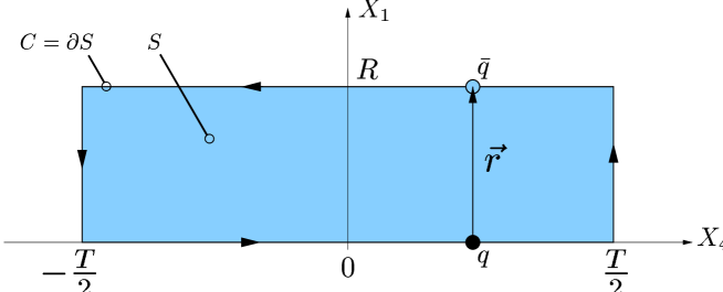
Figure 3.1: A static color dipole of size $R$ in the fundamental representation. The rectangular path $C$ of spatial extension $R$ and temporal extension $T$ indicates the world-line of the dipole described the Wegner-Wilson loop $W_{\mbox{\scriptsize N}_{c}}[C]$. The shaded area bounded by the loop $C=\partial S$ represents the minimal surface $S$ used to compute the static dipole potential.

illustrates a static color dipole in the fundamental representation $r=\mbox{N}_{c}$. The potential of the static color dipole is obtained from the VEV of the corresponding Wegner-Wilson loop [37, 79]

$$V_{r}(R)=-\lim_{T\to\infty}\frac{1}{T}\ln\langle W_{r}[C]\rangle_{\mbox{\scriptsize pot}}\ ,$$ (3.1)

where “pot” indicates the subtraction of the self-energy of the color sources. The static quark-antiquark potential $V_{\mbox{\scriptsize N}_{c}}$ is obtained from a loop in the fundamental representation ($r\!=\!\mbox{N}_{c}$) and the potential of a static gluino pair $V_{\mbox{\scriptsize N}_{c}^{2}\!-\!1}$ from a loop in the adjoint representation ($r\!=\!\mbox{N}_{c}^{2}\!-\!1$).

With our result for $\langle W_{r}[C]\rangle$, (2.14), obtained with the Gaussian approximation in the gluon field strength, the static potential reads

$$V_{r}(R)=\frac{C_{2}(r)}{2}\,\lim_{T\to\infty}\frac{1}{T}\,\chi_{SS\,\mbox{\scriptsize pot}}\ ,$$ (3.2)

with the self-energy subtracted, i.e. $\chi_{SS\,\mbox{\scriptsize pot}}:=\chi_{SS}-\chi_{SS\,\mbox{\scriptsize self}}$ (see Appendix B). According to the structure of the gluon field strength correlator, (2.12) and (2.42), there are perturbative ($P$) and non-perturbative ($N\!P$) contributions to the static potential

$$V_{r}(R)=\frac{C_{2}(r)}{2}\,\lim_{T\to\infty}\frac{1}{T}\,\left\{\chi_{SS\,\mbox{\scriptsize pot}}^{P}+\left(\chi_{SS\,\mbox{\scriptsize pot}}^{N\!P\,\,nc}+\chi_{SS\,\mbox{\scriptsize pot}}^{N\!P\,\,c}\right)\right\}\ ,$$ (3.3)

where the explicit form of the $\chi$ - functions is given in (B.9), (B.28), and (B.37).

The perturbative contribution to the static potential describes the color Yukawa potential (which reduces to the color Coulomb potential [80] for $m_{G}=0$)

$$V_{r}^{P}(R)=-C_{2}(r)\,\frac{g^{2}(R)}{4\pi R}\exp[-m_{G}R]\ .$$ (3.4)

Here we have used the result for $\chi_{SS\,\mbox{\scriptsize pot}}^{P}$ given in (B.37) and the perturbative correlation function

$$D^{\prime\,(3)}_{P}(\vec{Z}^{2}):=\int\frac{d^{4}K}{(2\pi)^{3}}\,e^{iKZ}\,\tilde{D}^{\prime\,(3)}_{P}(K^{2})\,\delta(K_{4})=-\,\frac{\exp[-\,m_{G}\,|\vec{Z}|]}{4\pi|\vec{Z}|}$$ (3.5)

which is obtained from the massive gluon propagator (2.43). As shown below, the perturbative contribution dominates the static potential for small dipoles sizes $R$.

The non-perturbative contributions to the static potential, the non-confining component ($nc$) and the confining component ($c$), read

$$V_{r}^{N\!P\,\,nc}(R) = C_{2}(r)\,\,\frac{\pi^{2}G_{2}(1-\kappa)}{3(N_{c}^{2}-1)}\,\,D_{1}^{\prime\,(3)}(R^{2})$$ (3.6)

$$V_{r}^{N\!P\,\,c}(R) = C_{2}(r)\,\,\frac{\pi^{2}G_{2}\kappa}{3(N_{c}^{2}-1)}\,\,\int_{0}^{R}\!\!d\rho\,(R-\rho)\,D^{(3)}(\rho^{2})\ ,$$ (3.7)

where we have used the results for $\chi_{SS\,\mbox{\scriptsize pot}}^{N\!P\,\,nc}$ and $\chi_{SS\,\mbox{\scriptsize pot}}^{N\!P\,\,c}=\chi_{SS}^{N\!P\,\,c}$ given respectively in (B.28) and (B.9) obtained with the minimal surface, i.e. the planar surface bounded by the loop as indicated by the shaded area in Fig. 3.1. With the exponential correlation function (2.50), the correlation functions in (3.6) and (3.7) read

$$D^{\prime\,(3)}_{1}(\vec{Z}^{2}) \!\!:=\!\! \int\frac{d^{4}K}{(2\pi)^{3}}\,e^{iKZ}\,\tilde{D}^{\prime\,(3)}_{1}(K^{2})\,\delta(K_{4})\,\,=\,\,-\,a\,|\vec{Z}|^{2}\,K_{2}[|\vec{Z}|/a]\ ,$$ (3.8)

$$D^{(3)}(\vec{Z}^{2}) \!\!:=\!\! \int\frac{d^{4}K}{(2\pi)^{3}}\,e^{iKZ}\,\tilde{D}(K^{2})\,\delta(K_{4})\,\,=\,\,2\,|\vec{Z}|\,K_{1}[|\vec{Z}|/a]\ .$$ (3.9)

For large dipole sizes, $R\gtrsim 0.5\ \mbox{fm}$, the non-confining contribution (3.6) vanishes exponentially while the confining contribution (3.7) – as anticipated – leads to confinement [27], i.e. the confining linear increase,

$$V_{r}^{N\!P\,\,c}(R)\Big{|}_{R\,\gtrsim\,0.5\,\mbox{\scriptsize fm}}=\sigma_{r}R+\mbox{const.}\ .$$ (3.10)

Thus, the QCD string tension is given by the confining SVM component [27]: For a color dipole in the $SU(N_{c})$ representation $r$, it reads

$$\sigma_{r}=C_{2}(r)\,\,\frac{\pi^{3}G_{2}\kappa}{48}\int_{0}^{\infty}dZ^{2}D(Z^{2})=C_{2}(r)\,\,\frac{\pi^{3}\kappa G_{2}a^{2}}{24}\ ,$$ (3.11)

where the exponential correlation function (2.50) is used in the final step. Since the string tension can be computed from first principles within lattice QCD [63], relation (3.11) puts an important constraint on the three parameters of the non-perturbative QCD vacuum $a$, $G_{2}$, and $\kappa$. With the values for $a$, $G_{2}$, and $\kappa$ given in (2.51), that are used throughout this work, one obtains for the string tension of the $SU(3)$ quark-antiquark potential ($r=3$) a reasonable value of

$$\sigma_{3}=0.22\,\mbox{GeV}^{2}\equiv 1.12\,\mbox{GeV}/\mbox{fm}\ .$$ (3.12)

The static $SU(N_{c}=3)$ quark-antiquark potential $V_{\mbox{\scriptsize N}_{c}}(R)=V_{3}(R)$ is shown as a function of the quark-antiquark separation $R$ in Fig. 3.2,

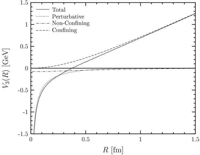
Figure 3.2: The static $SU(N_{c}=3)$ quark-antiquark potential $V_{\mbox{\scriptsize N}_{c}}(R)=V_{3}(R)$ as a function of the quark-antiquark separation $R$. The solid, dotted, and dashed lines indicate the full static potential and its perturbative and non-perturbative contributions, respectively. For small quark-antiquark separations, $R\lesssim 0.5\,\mbox{fm}$, the perturbative contribution dominates and gives rise to the well-known color Coulomb behavior at small distances. For medium and large quark-antiquark separations, $R\gtrsim 0.5\,\mbox{fm}$, the non-perturbative contribution dominates and leads to the confining linear rise of the static potential. As our model is working in the quenched approximation, string breaking cannot be described, which is expected to stop the linear increase for $R\,\gtrsim\,1\,\mbox{fm}$ [81, 63].

where the solid, dotted, and dashed lines indicate the full static potential and its perturbative and non-perturbative contributions, respectively. For small quark-antiquark separations $R\lesssim 0.5\,\mbox{fm}$, the perturbative contribution dominates giving rise to the well-known color Coulomb behavior. For medium and large quark-antiquark separations $R\gtrsim 0.5\,\mbox{fm}$, the non-perturbative contribution dominates and leads to the confining linear rise of the static potential. The transition from perturbative to string behavior takes place at source separations of about $0.5\,\mbox{fm}$ in agreement with the recent results of Lüscher and Weisz [40]. This supports our value for the gluon mass $m_{G}=m_{\rho}=0.77\,\mbox{GeV}$ which is only important around $R\approx 0.4\,\mbox{fm}$, i.e. for the interplay between perturbative and non-perturbative physics. For $R\lesssim 0.3\,\mbox{fm}$ and $R\gtrsim 0.5\,\mbox{fm}$, the effect of the gluon mass, introduced as an IR regulator in our perturbative component, is negligible. String breaking is expected to stop the linear increase for $R\,\gtrsim\,1\,\mbox{fm}$ where lattice investigations show deviations from the linear rise in full QCD [81, 63]. As our model is working in the quenched approximation, string breaking through dynamical quark-antiquark production is excluded.

As can be seen from (3.2), the static potential shows Casimir scaling which emerges in our approach as a trivial consequence of the Gaussian approximation used to truncate the cumulant expansion (2.7). Indeed, the Casimir scaling hypothesis [82] has been verified to high accuracy for $SU(3)$ on the lattice [83, 84] (see also Fig. 3.3). These lattice results have been interpreted as a strong hint towards Gaussian dominance in the QCD vacuum and thus as evidence for a strong suppression of higher cumulant contributions [85, 86]. In contrast to our model, the instanton model can neither describe Casimir scaling [86] nor the linear rise of the confining potential [87].

Figure 3.3

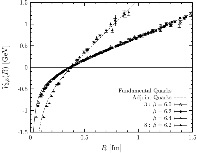
Figure 3.3: The static $SU(N_{c}=3)$ potential of color dipoles in the fundamental representation $V_{3}(R)$ (solid line) and adjoint representation $V_{8}(R)$ (dashed line) as a function of the dipole size $R$ in comparison to $SU(3)$ lattice data for $\beta=6.0$, 6.2, and 6.4 [84, 63]. The model results are in good agreement with the lattice data. This particularly holds for the obtained Casimir scaling behavior.

shows the static $SU(N_{c}=3)$ potential for fundamental sources $V_{\mbox{\scriptsize N}_{c}}(R)=V_{3}(R)$ (solid line) and adjoint sources $V_{\mbox{\scriptsize N}_{c}^{2}\!-\!1}(R)=V_{8}(R)$ (dashed line) as a function of the dipole size $R$ in comparison to $SU(3)$ lattice data [84, 63]. The model results are in good agreement with the lattice data. In particular, the obtained Casimir scaling behavior is strongly supported by $SU(3)$ lattice data [83, 84]. This, however, points also to a shortcoming of our model: From Eq. (3.2) and Fig. 3.3 it is clear that string breaking is neither described for fundamental nor for adjoint dipoles in our model which indicates that not only dynamical fermions (quenched approximation) are missing but also some gluon dynamics.

3.2 Chromo-Field Distributions of Color Dipoles

As already explained in Sec. 3.1, the static color dipole – two static color sources separated by a distance $R$ in a net color singlet state – is described by a Wegner-Wilson loop $W_{r}[C]$ with a rectangular path $C$ of spatial extension $R$ and temporal extension $T\to\infty$ (cf. Fig. 3.1) where $r$ indicates the $SU(N_{c})$ representation of the considered sources. A second small quadratic loop or plaquette in the fundamental representation placed at the space-time point $X$ with side length $R_{P}\to 0$ and oriented along the $\alpha\beta$-axes

$$P_{\mbox{\scriptsize N}_{c}}^{\alpha\beta}(X)=\tilde{\mbox{Tr}}_{\mbox{\scriptsize N}_{c}}\exp\!\!\left[-ig\oint_{C_{P}}\!\!\!dZ_{\mu}{\cal G}_{\mu}^{a}(Z)t_{\mbox{\scriptsize N}_{c}}^{a}\right]=1-R_{P}^{4}\frac{g^{2}}{4N_{c}}{\cal G}_{\alpha\beta}^{a}(X){\cal G}_{\alpha\beta}^{a}(X)+{\cal O}(R_{P}^{6})$$ (3.13)

is needed – as a “Hall probe” – to calculate the chromo-field distributions at the space-time point $X$ caused by the static sources [88, 89]

$$\Delta G_{r\,\alpha\beta}^{2}(X) := \Big{\langle}\frac{g^{2}}{4\pi^{2}}{\cal G}_{\alpha\beta}^{a}(X){\cal G}_{\alpha\beta}^{a}(X)\Big{\rangle}_{W_{r}[C]}-\Big{\langle}\frac{g^{2}}{4\pi^{2}}{\cal G}_{\alpha\beta}^{a}(X){\cal G}_{\alpha\beta}^{a}(X)\Big{\rangle}_{\mbox{\scriptsize vac}}$$ (3.14)

$$= -\,\lim_{R_{P}\to 0}\frac{1}{R_{P}^{4}}\frac{N_{c}}{\pi^{2}}\left[\frac{\langle W_{r}[C]P_{\mbox{\scriptsize N}_{c}}^{\alpha\beta}(X)\rangle}{\langle W_{r}[C]\rangle}-\langle P_{\mbox{\scriptsize N}_{c}}^{\alpha\beta}(X)\rangle\right]$$ (3.15)

with no summation over $\alpha$ and $\beta$ in (3.13), (3.14), and (3.15). In definition (3.14) $\langle\ldots\rangle_{W_{r}[C]}$ indicates the VEV in the presence of the static color dipole while $\langle\ldots\rangle_{\mbox{\scriptsize vac}}$ indicates the VEV in the absence of any color sources. Depending on the plaquette orientation indicated by $\alpha$ and $\beta$, one obtains from (3.15) the squared components of the chromo-electric and chromo-magnetic field at the space-time point $X$

$$\Delta G_{r\,\alpha\beta}^{2}(X)=\frac{g^{2}}{4\pi^{2}}\left(\begin{array}[]{cccc}0&B_{z}^{2}&B_{y}^{2}&E_{x}^{2}\\ B_{z}^{2}&0&B_{x}^{2}&E_{y}^{2}\\ B_{y}^{2}&B_{x}^{2}&0&E_{z}^{2}\\ E_{x}^{2}&E_{y}^{2}&E_{z}^{2}&0\end{array}\right)(X)\ ,$$ (3.16)

i.e. space-time plaquettes ($\alpha\beta=i4$) measure chromo-electric fields and space-space plaquettes ($\alpha\beta=ij$) chromo-magnetic fields. As shown in Fig. 3.4, we place the static color sources on the $X_{1}$-axis at $(X_{1}=\pm R/2,0,0,X_{4})$ and use the following notation plausible from symmetry arguments

$$E_{\parallel}^{2}=E_{x}^{2}\ ,\quad E_{\perp}^{2}=E_{y}^{2}=E_{z}^{2}\ ,\quad B_{\parallel}^{2}=B_{x}^{2}\ ,\quad B_{\perp}^{2}=B_{y}^{2}=B_{z}^{2}\ .$$ (3.17)

Figure 3.4 illustrates also the plaquette $P_{\mbox{\scriptsize N}_{c}}^{14}(X)$ at $X=(X_{1},X_{2},0,0)$ needed to compute $E_{\parallel}^{2}(X)$. Due to symmetry arguments, the complete information on the chromo-field distributions is obtained from plaquettes in “transverse” space $X=(X_{1},X_{2},0,0)$ with four different orientations, $\alpha\beta=14,\,24,\,13,\,23$, cf. (3.17).

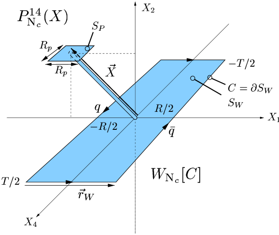
Figure 3.4: The plaquette-loop geometry needed to compute the squared chromo-electric field $E_{\parallel}^{2}(X)$ generated by a static color dipole in the fundamental $SU(N_{c})$ representation ($r=\mbox{N}_{c}$). The rectangular path $C$ indicates the world-line of the static dipole described the Wegner-Wilson loop $W_{\mbox{\scriptsize N}_{c}}[C]$. The square with side length $R_{P}$ illustrates the plaquette $P_{\mbox{\scriptsize N}_{c}}^{14}(X)$. The shaded areas represent the minimal surfaces used in our computation of the chromo-field distributions. The thin tube allows us to compare the gluon field strengths in surface $S_{P}$ with the gluon field strengths in surface $S_{W}$.

The energy and action density distributions around a static color dipole in the $SU(N_{c})$ representation $r$ are given by the squared chromo-field distributions

$$\varepsilon_{r}(X) = \frac{1}{2}\left(-\vec{E}^{2}(X)+\vec{B}^{2}(X)\right)$$ (3.18)

$$\mathit{s}_{r}(X) = -\frac{1}{2}\left(\vec{E}^{2}(X)+\vec{B}^{2}(X)\right)$$ (3.19)

with signs according to Euclidean space-time conventions. Low-energy theorems that relate the energy and action stored in the chromo-fields of the static color dipole to the corresponding ground state energy are discussed in the next section.

For the chromo-field distributions of a static color dipole in the fundamental representation of $SU(N_{c})$, i.e. a static quark-antiquark pair, we obtain with our results for the VEV of one loop (2.14) and the correlation of two loops in the fundamental representation (2.35)

$$\Delta G_{\mbox{\scriptsize N}_{c}\,\alpha\beta}^{2}(X)=-\lim_{R_{P}\to 0}\frac{1}{R_{P}^{4}}\frac{N_{c}}{\pi^{2}}\exp\left[-\frac{C_{2}(\!\mbox{N}_{c}\!)}{2}\,\chi_{S_{P}S_{P}}\right]$$ (3.20)

$$\hskip 56.9055pt\times\Bigg{(}\frac{N_{c}+1}{2N_{c}}\exp\!\left[-\frac{N_{c}-1}{2N_{c}}\chi_{S_{P}S_{W}}\right]+\frac{N_{c}-1}{2N_{c}}\exp\!\left[\frac{N_{c}+1}{2N_{c}}\chi_{S_{P}S_{W}}\right]-1\Bigg{)}$$

where $\chi_{S_{i}S_{j}}$ is defined in (2.27). The subscripts $P$ and $W$ indicate surface integrations to be performed over the surfaces spanned by the plaquette and the Wegner-Wilson-loop, respectively. Choosing the surfaces – as illustrated by the shaded areas in Fig. 3.4 – to be the minimal surfaces connected by an infinitesimal thin tube (which gives no contribution to the integrals) it is clear that $\chi_{S_{P}S_{P}}\propto R_{P}^{4}$ and $\chi_{S_{P}S_{W}}\propto R_{P}^{2}$. Being interested in the chromo-fields at the space-time point $X$, the extension of the quadratic plaquette is taken to be infinitesimally small, $R_{P}\rightarrow 0$, so that one can expand the exponential functions and keep only the term of lowest order in $R_{P}$

$$\Delta G_{\mbox{\scriptsize N}_{c}\,\alpha\beta}^{2}(X)=-\,C_{2}(\!\mbox{N}_{c}\!)\,\lim_{R_{P}\to 0}\frac{1}{R_{P}^{4}}\,\frac{1}{4\pi^{2}}\,\chi_{S_{P}S_{W}}^{2}\ .$$ (3.21)

This result – obtained with the matrix cumulant expansion in a very straightforward way – agrees exactly with the result derived in [28] with the expansion method. Indeed, the expansion method agrees for small $\chi$-functions with the matrix cumulant expansion (Berger-Nachtmann approach) used in this work but breaks down for large $\chi$-functions, where the matrix cumulant expansion is still applicable.

The chromo-field distributions of a static color dipole in the adjoint representation of $SU(N_{c})$, i.e. a static gluino pair, are computed analogously. Using our result (2.40) for the correlation of one loop in the fundamental representation (plaquette) with one loop in the adjoint representation (static sources), one obtains

$$\!\!\!\!\!\!\!\!\Delta G_{\mbox{\scriptsize N}_{c}^{2}\!-\!1\,\alpha\beta}^{2}(X)=-\lim_{R_{P}\to 0}\frac{1}{R_{P}^{4}}\frac{N_{c}}{\pi^{2}}\exp\left[-\frac{C_{2}(\!\mbox{N}_{c}\!)}{2}\chi_{S_{P}S_{P}}\right]\,\Bigg{(}\!\frac{1}{N_{c}^{2}\!-\!1}\,\exp\!\Big{[}\frac{N_{c}}{2}\,\chi_{S_{P}S_{W}}\Big{]}$$

$$\hskip 42.67912pt+\,\frac{N_{c}\!+\!2}{2(N_{c}\!+\!1)}\exp\!\Big{[}\!-\frac{1}{2}\,\chi_{S_{P}S_{W}}\Big{]}+\frac{N_{c}\!-\!2}{2(N_{c}\!-\!1)}\exp\!\Big{[}\frac{1}{2}\,\chi_{S_{P}S_{W}}\Big{]}-1\!\Bigg{)}$$ (3.22)

which reduces – as explained for sources in the fundamental representation – to

$$\Delta G_{\mbox{\scriptsize N}_{c}^{2}\!-\!1\,\alpha\beta}^{2}(X)=-\,C_{2}(\!\mbox{N}_{c}^{2}\!-\!1\!)\,\lim_{R_{P}\to 0}\frac{1}{R_{P}^{4}}\,\frac{1}{4\pi^{2}}\,\chi_{S_{P}S_{W}}^{2}\ .$$ (3.23)

Thus, the squared chromo-electric fields of an adjoint dipole differ from those of a fundamental dipole only in the eigenvalue of the corresponding quadratic Casimir operator $C_{2}(r)$. In fact, Casimir scaling of the chromo-field distributions holds for dipoles in any representation $r$ of $SU(N_{c})$ in our model. As can be seen with the low-energy theorems discussed below, this is in line with the Casimir scaling of the static dipole potential found in the previous section. Besides lattice investigations that show Casimir scaling of the static dipole potential to high accuracy in $SU(3)$ [83, 84], Casimir scaling of the chromo-field distributions has been considered on the lattice as well but only for $SU(2)$ [90]. Here only slight deviations from the Casimir scaling hypothesis have been found that were interpreted as hints towards adjoint quark screening.

In our model the shape of the field distributions around the color dipole is identical for all $SU(N_{c})$ representations $r$ and given by $\chi_{S_{P}S_{W}}^{2}$. This again illustrates the shortcoming of our model discussed in the previous section. Working in the quenched approximation, one expects a difference between fundamental and adjoint dipoles: string breaking cannot occur in fundamental dipoles as dynamical quark-antiquark production is excluded but should be present for adjoint dipoles because of gluonic vacuum polarization. Comparing (3.21) with (3.23) it is clear that this difference is not described in our model. In fact, as shown in Sec. 3.1, string breaking is neither described for fundamental nor for adjoint dipoles. Interestingly, even on the lattice there has been no striking evidence for adjoint quark screening in quenched QCD [91]. It is even conjectured that the Wegner-Wilson loop operator is not suited to studies of string breaking [92].

In the LLCM there are perturbative ($P$) and non-perturbative ($N\!P$) contributions to the chromo-electric fields according to the structure of the gluon field strength correlator, (2.12) and (2.42),

$$\Delta G_{r\,\alpha\beta}^{2}(X) = -C_{2}(r)\,\lim_{R_{P}\to 0}\frac{1}{R_{P}^{4}}\,\frac{1}{\pi^{2}}\,$$

$$\times\left\{\left(\chi_{S_{P}S_{W}}^{P}(X)\right)_{\alpha\beta}^{2}+\left[\left(\chi_{S_{P}S_{W}}^{N\!P\,nc}(X)\right)_{\alpha\beta}+\left(\chi_{S_{P}S_{W}}^{N\!P\,c}(X)\right)_{\alpha\beta}\right]^{2}\right\}$$

where we have demanded the non-interference of perturbative and non-perturbative correlations in line with the Minkowskian applications of our model [23, 25, 24, 26]. In the following we give only the final results of the $\chi$ - functions for the minimal surfaces shown in Fig. 3.4. Details on their derivation can be found in Appendix B.

The perturbative contribution ($P$) described by massive gluon exchange leads, of course, to the well-known color Yukawa field that reduces to the color Coulomb field for $m_{g}=0$. It contributes only to the chromo-electric fields, $E_{\parallel}^{2}=E_{x}^{2}$ ($\alpha\beta=14$) and $E_{\perp}^{2}=E_{y}^{2}=E_{z}^{2}$ ($\alpha\beta=24$), and reads explicitly for $X=(X_{1},X_{2},0,0)$

$$\!\!\!\!\!\!\!\!\!\!\!\!\left(\chi_{S_{P}S_{W}}^{P}(X)\right)_{14} \!\!=\!\! -\,\frac{R_{P}^{2}}{2}\!\int_{-\infty}^{\infty}\!\!\!d\tau\left\{(X_{1}-R/2)\,g^{2}(Z_{1A}^{2})\,D_{P}(Z_{1A}^{2})\right.$$ (3.25)

$$\hphantom{-\,\frac{R_{P}^{2}}{2}\!\int_{-\infty}^{\infty}\!\!\!d\tau\Big{(}}\left.-\,(X_{1}+R/2)\,g^{2}(Z_{1C}^{2})\,D_{P}(Z_{1C}^{2})\right\}$$

$$\!\!\!\!\!\!\!\!\!\!\!\!\left(\chi_{S_{P}S_{W}}^{P}(X)\right)_{24} \!\!=\!\! -\,\frac{R_{P}^{2}}{2}\!\int_{-\infty}^{\infty}\!\!\!d\tau\,X_{2}\left\{g^{2}(Z_{1A}^{2})\,D_{P}(Z_{1A}^{2})-g^{2}(Z_{1C}^{2})\,D_{P}(Z_{1C}^{2})\right\}$$ (3.26)

with the perturbative correlation function (2.45), the running coupling (2.47), and

$$Z_{1A}^{2}=\left(X_{1}\!-\!\frac{R}{2}\right)^{2}+X_{2}^{2}+\tau^{2}\quad\mbox{and}\quad Z_{1C}^{2}=\left(X_{1}\!+\!\frac{R}{2}\right)^{2}+X_{2}^{2}+\tau^{2}\ .$$ (3.27)

The non-confining non-perturbative contribution ($N\!P\,nc$) has the same structure as the perturbative contribution – as expected from the identical tensor structure – but differs, of course, in the prefactors and the correlation function, $D_{1}\neq D_{p}$. Its contributions to the chromo-electric fields $E_{\parallel}^{2}=E_{x}^{2}$ ($\alpha\beta=14$) and $E_{\perp}^{2}=E_{y}^{2}=E_{z}^{2}$ ($\alpha\beta=24$) read for $X=(X_{1},X_{2},0,0)$

$$\left(\chi_{S_{P}S_{W}}^{N\!P\,\,nc}(X)\right)_{14} = -\,\frac{R_{P}^{2}\pi^{2}G_{2}(1\!-\!\kappa)}{6\,(N_{c}^{2}\!-\!1)}\!\int_{-\infty}^{\infty}\!\!\!d\tau\Big{\{}(X_{1}-R/2)\,D_{1}(Z_{1A}^{2})$$ (3.28)

$$\hphantom{-\,\frac{R_{P}^{2}\pi^{2}G_{2}}{6\,(N_{c}^{2}\!-\!1)}}-\,(X_{1}+R/2)\,D_{1}(Z_{1C}^{2})\Big{\}}$$

$$\left(\chi_{S_{P}S_{W}}^{N\!P\,\,nc}(X)\right)_{24} = -\,\frac{R_{P}^{2}\pi^{2}G_{2}(1\!-\!\kappa)}{6\,(N_{c}^{2}\!-\!1)}\!\int_{-\infty}^{\infty}\!\!\!d\tau\,X_{2}\Big{\{}D_{1}(Z_{1A}^{2})-D_{1}(Z_{1C}^{2})\Big{\}}$$ (3.29)

with the exponential correlation function (2.50) and $Z_{1A}^{2}$ and $Z_{1C}^{2}$ as given in (3.27).

The confining non-perturbative contribution ($N\!P\,c$) has a different structure that leads to confinement and flux-tube formation. It gives only contributions to the chromo-electric field $E_{\parallel}^{2}=E_{x}^{2}$ ($\alpha\beta=14$) that read for $X=(X_{1},X_{2},0,0)$

$$\left(\chi_{S_{P}S_{W}}^{N\!P\,\,c}(X)\right)_{14} = R_{P}^{2}R\frac{\pi^{2}G_{2}\kappa}{3\,(N_{c}^{2}\!-\!1)}\int_{0}^{1}d\rho\,D^{(3)}(\vec{Z_{\perp}}^{2})\ ,$$ (3.30)

with the correlation function given in (3.9) as derived from the exponential correlation function (2.50), and

$$\vec{Z}_{\perp}^{2}=[X_{1}+(1/2-\rho)R]^{2}+X_{2}^{2}\ .$$ (3.31)

In our model there are no contributions to the chromo-magnetic fields, i.e. the static color charges do not affect the magnetic background field

$$B_{\parallel}^{2}=B_{x}^{2}=0\quad\mbox{and}\quad B_{\perp}^{2}=B_{y}^{2}=B_{z}^{2}=0\ ,$$ (3.32)

which can be seen from the corresponding plaquette-loop geometries as pointed out in Appendix B. Thus, the energy and action densities are identical in our approach and completely determined by the squared chromo-electric fields

$$\varepsilon_{r}(X)\,\,=\,\,\mathit{s}_{r}(X)\,\,=\,\,-\frac{1}{2}\,\vec{E}^{2}(X)\ .$$ (3.33)

This picture is in agreement with other effective theories of confinement such as the ‘t Hooft-Mandelstam picture [93] or dual QCD [94] and, indeed, a relation between the dual Abelian Higgs model and the SVM has been established [95]. In contrast, lattice investigations work at scales at which the chromo-electric and chromo-magnetic fields are of similar magnitude [96, 44]. Using low-energy theorems, we will see in the next section, that the vanishing of the chromo-magnetic fields determines the value of the $\beta$-function at the renormalization scale at which the non-perturbative component of our model is working.

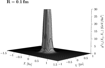
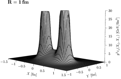
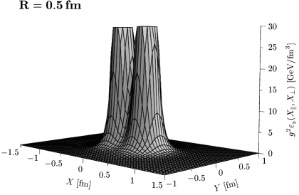
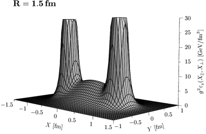
Figure 3.5: Energy density distributions $g^{2}\varepsilon_{3}(X_{1},X_{2}\!=\!X_{3})$ generated by a color dipole in the fundamental $SU(3)$ representation ($r\!=\!3$) for quark-antiquark separations of $R=0.1,\,0.5,\,1$ and $1.5\,\mbox{fm}$. Flux-tube formation leads to the confining QCD string with increasing dipole size $R$.

In Fig. 3.5 the energy density distributions $g^{2}\varepsilon_{3}(X_{1},X_{2}\!=\!X_{3})$ generated by a color dipole in the fundamental $SU(3)$ representation ($r\!=\!3$) are shown for quark-antiquark separations of $R=0.1,\,0.5,\,1$ and $1.5\,\mbox{fm}$. With increasing dipole size $R$, one sees explicitly the formation of the flux tube which represents the confining QCD string.

The longitudinal and transverse energy density profiles generated by a color dipole in the fundamental representation ($r=3$) of $SU(N_{c}=3)$ are shown for quark-antiquark separations (dipole sizes) of $R=0.1,\,0.5,\,1$ and $1.5\,\mbox{fm}$ in Figs. 3.6 and 3.7. The perturbative and non-perturbative contributions are given in the dotted and dashed lines, respectively, and the sum of both in the solid lines. The open and filled circles indicate the quark and antiquark positions. As can be seen from (3.15) and (3.16), we cannot compute the energy density separately but only the product $g^{2}\varepsilon_{r}(X)$. Nevertheless, a comparison of the total energy stored in chromo-electric fields to the ground state energy of the color dipole via low-energy theorems yields $g^{2}=10.2$ $(\equiv\alpha_{s}=0.81)$ for the non-perturbative SVM component as shown in the next section.

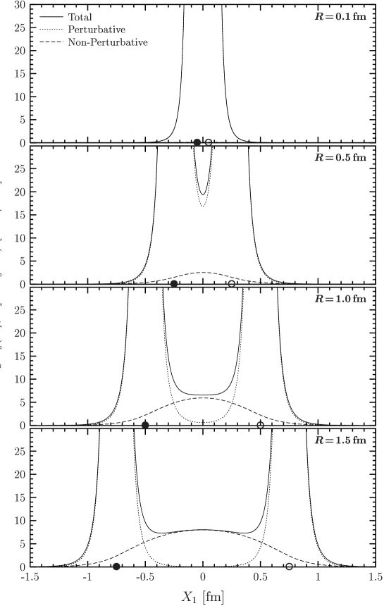
Figure 3.6: Longitudinal energy density profiles $g^{2}\varepsilon_{3}(X_{1},X_{2}\!=\!X_{3}\!=\!0)$ generated by a color dipole in the fundamental $SU(3)$ representation ($r\!=\!3$) for quark-antiquark separations of $R=0.1,\,0.5,\,1$ and $1.5\,\mbox{fm}$. The dotted and dashed lines give the perturbative and non-perturbative contributions, respectively, and the solid lines the sum of both. The open and filled circles indicate the quark and antiquark positions. For small dipoles, $R=0.1\,\mbox{fm}$, perturbative physics dominates and non-perturbative correlations are negligible. For large dipoles, $R\gtrsim 1\,\mbox{fm}$, the formation the confining string (flux tube) can be seen which dominates the chromo-electric fields between the color sources.

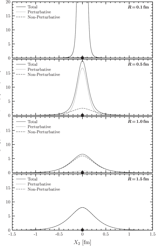
Figure 3.7: Transverse energy density profiles $g^{2}\varepsilon_{3}(X_{2},X_{1}\!=\!X_{3}\!=\!0)$ generated by a color dipole in the fundamental $SU(3)$ representation ($r\!=\!3$) for quark-antiquark separations of $R=0.1,\,0.5,\,1$ and $1.5\,\mbox{fm}$. The dotted and dashed lines give the perturbative and non-perturbative contributions, respectively, and the solid lines the sum of both. The filled circles indicate the positions of the color sources. For small dipoles, $R=0.1\,\mbox{fm}$, perturbative physics dominates and non-perturbative correlations are negligible. For large dipoles, $R\gtrsim 1\,\mbox{fm}$, the formation the confining string (flux tube) can be seen which dominates the chromo-electric fields between the color sources.

In Figs. 3.6 and 3.7 the formation of the confining string (flux tube) with increasing source separations $R$ can again be seen explicitly: For small dipoles, $R=0.1\,\mbox{fm}$, perturbative physics dominates and non-perturbative correlations are negligible. For large dipoles, $R\gtrsim 1\,\mbox{fm}$, the non-perturbative correlations lead to formation of a narrow flux tube which dominates the chromo-electric fields between the color sources.

Figure 3.8

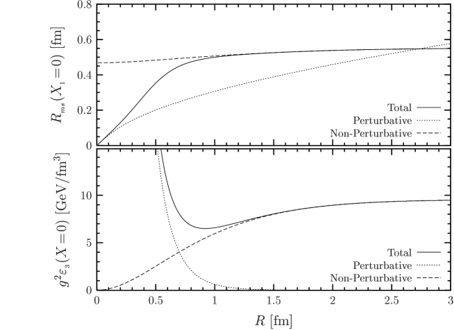
Figure 3.8: Root mean squared radius $R_{ms}$ of the flux tube and energy density in the center of a fundamental $SU(3)$ dipole $g^{2}\varepsilon_{3}(X=0)$ as a function of the dipole size $R$. Perturbative and non-perturbative contributions are given respectively in the dotted and dashed lines and the sum of both in the solid lines. For large $R$, both the width and height of the flux tube in the central region are governed completely by non-perturbative physics and saturate respectively at $R_{ms}^{R\to\infty}\approx 0.55\,\mbox{fm}$ and $\varepsilon_{3}^{R\to\infty}(X=0)\approx 1\,\mbox{GeV}/\mbox{fm}^{3}$. The latter value is extracted with the result $g^{2}=10.2$ deduced from low-energy theorems in the next section.

shows the evolution of the transverse width (upper plot) and height (lower plot) of the flux tube in the central region of the Wegner-Wilson loop as a function of the dipole size $R$ where perturbative and non-perturbative contributions are given in the dotted and dashed lines, respectively, and the sum of both in the solid lines. The width of the flux tube is best described by the root mean squared ($ms$) radius

$$R_{ms}=\sqrt{\frac{\int dX_{\perp}\,X_{\perp}^{3}\,g^{2}\varepsilon_{r}(X_{1}=0,X_{\perp})}{\int dX_{\perp}\,X_{\perp}\,g^{2}\varepsilon_{r}(X_{1}=0,X_{\perp})}}\ ,$$ (3.34)

which is universal for dipoles in all $SU(N_{c})$ representations $r$ as the Casimir factors divide out. The height of the flux tube is given by the energy density in the center of the considered dipole, $g^{2}\varepsilon_{r}(X=0)$. For large source separations, $R\gtrsim 1\,\mbox{fm}$, both the width and height of the flux tube in the central region of the Wegner-Wilson loop are governed completely by non-perturbative physics and saturate for a fundamental $SU(3)$ dipole ($r=\mbox{N}_{c}=3$) at reasonable values of

$$R_{ms}^{R\to\infty}\approx 0.55\,\mbox{fm}\quad\mbox{and}\quad\varepsilon_{3}^{R\to\infty}(X=0)\approx 1\,\mbox{GeV}/\mbox{fm}^{3}\quad\mbox{with}\quad g^{2}=10.2\ .$$ (3.35)

Note that the qualitative features of the non-perturbative SVM component do not depend on the specific choice for the parameters, surfaces, and correlation functions and have already been discussed with the pyramid mantle choice of the surface and different correlation functions in the first investigation of flux-tube formation in the SVM [28]. The quantitative results, however, are sensitive to the parameter values, the surface choice, and the correlation functions and are presented above with the LLCM parameters, the minimal surfaces, and the exponential correlation function [22].

3.3 Low-Energy Theorems

Many low-energy theorems have been derived in continuum theory by Novikov, Shifman, Vainshtein, and Zakharov [97] and in lattice gauge theory by Michael [41]. Here we consider the energy and action sum rules – known in lattice QCD as Michael sum rules – that relate the energy and action stored in the chromo-fields of a static color dipole to the corresponding ground state energy [37, 79]

$$E_{r}(R)=-\lim_{T\to\infty}\frac{1}{T}\ln\langle W_{r}[C]\rangle\ .$$ (3.36)

In their original form [41], however, the Michael sum rules are incomplete [29, 42]. In particular, significant contributions to the energy sum rule from the trace anomaly of the energy-momentum tensor have been found [42] that modify the naively expected relation in line with the importance of the trace anomaly found for hadron masses [98]. Taking all these contributions into account, the energy and action sum rule read respectively [42, 43, 44]

$$E_{r}(R)=\int d^{3}X\,\varepsilon_{r}(X)-\frac{1}{2}\frac{\beta(g)}{g}\int d^{3}X\,\mathit{s}_{r}(X)$$ (3.37)

$$E_{r}(R)+R\,\frac{\partial E_{r}(R)}{\partial R}=-\frac{2\beta(g)}{g}\int d^{3}X\,\mathit{s}_{r}(X)$$ (3.38)

where $\beta(g)=\mu\partial g/\partial\mu$ with the renormalization scale $\mu$. Inserting (3.38) into (3.37), we find the following relation between the total energy stored in the chromo-fields $E_{r}^{\mbox{\scriptsize tot}}(R)$ and the ground state energy $E_{r}(R)$

$$E_{r}^{\mbox{\scriptsize tot}}(R):=\int d^{3}X\,\varepsilon_{r}(X)=\frac{1}{4}\left(3\,E_{r}(R)-R\frac{\partial E_{r}(R)}{\partial R}\right)\ .$$ (3.39)

The difference from the naive expectation that the full ground state energy of the static color sources is stored in the chromo-fields is due to the trace anomaly contribution [42] described by the second term on the right-hand side (rhs) of (3.37).

With the low energy theorems (3.38) and (3.39) the ratio of the integrated squared chromo-magnetic to the integrated squared chromo-electric field distributions can be derived

$$Q(R):=\frac{\int d^{3}X\vec{B}^{2}(X)}{\int d^{3}X\vec{E}^{2}(X)}=\frac{\left(2+6\,\beta(g)/g\right)\,E_{r}(R)+\left(1-\beta(g)/g\right)\,R\,\frac{\partial E_{r}(R)}{\partial R}}{\left(2-6\,\beta(g)/g\right)\,E_{r}(R)+\left(1+\beta(g)/g\right)\,R\,\frac{\partial E_{r}(R)}{\partial R}}\ ,$$ (3.40)

which becomes for $E_{r}(R)=\sigma_{r}R+E_{\mbox{\scriptsize self}}$ after subtraction of the self-energy contributions, i.e. the linear potential $V_{r}(R)=\sigma_{r}R$ with string tension $\sigma_{r}$ in the considered representation $r$,

$$Q(R)\Big{|}_{V_{r}(R)=\sigma_{r}R}=\frac{2+\beta(g)/g}{2-\beta(g)/g}\ .$$ (3.41)

In our model there are no contributions to the chromo-magnetic fields (3.32) so that – as already discussed in the previous section – the energy and action densities are identical and completely determined by the squared chromo-electric fields (3.33). Since the non-perturbative SVM component of our model describes the confining linear potential for large source separations $R$, this allows us to determine from (3.41) immediately the value of the $\beta$ - function at the scale $\mu_{N\!P}$ at which the non-perturbative component is working

$$\frac{\beta(g)}{g}\Big{|}_{\mu=\mu_{N\!P}}=-2\ .$$ (3.42)

Concentrating on the confining non-perturbative component ($N\!Pc$) we now use (3.39) to determine the value of $\alpha_{s}=g^{2}/(4\pi)$ at which the non-perturbative SVM component is working. The rhs of (3.39) is obtained directly from the confining contribution to the static potential $E_{r}^{N\!Pc}(R)=V_{r}^{N\!Pc}(R)$ given in (3.7). The lhs of (3.39), however, involves a division by the a priori unknown value of $g^{2}$ after integrating $g^{2}\varepsilon_{r}(X)$ for the chromo-electric field of the confining non-perturbative component (3.30). As discussed in the previous section, we cannot compute the energy density separately but only the product $g^{2}\varepsilon_{r}(X)$. Adjusting the value of $g^{2}$ such that (3.39) is exactly fulfilled for source separations of $R=1.5\,\mbox{fm}$, we find that the non-perturbative component is working at the scale $\mu_{N\!P}$ at which

$$g^{2}(\mu_{N\!P})=10.2\quad\equiv\quad\alpha_{s}(\mu_{N\!P})=0.81\ .$$ (3.43)

As already mentioned in Sec. 2.3, we use this value as a practical asymptotic limit for the simple one-loop coupling (2.47) used in our perturbative component. Note that earlier SVM investigations along these lines have found a smaller value of $\alpha_{s}(\mu_{N\!P})=0.57$ with the pyramid mantle choice for the surface [28, 29] but were incomplete since only the contribution from the traceless part of the energy-momentum tensor has been considered in the energy sum rule.

In Fig. 3.9

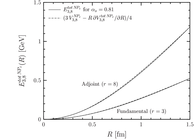
Figure 3.9: The total energy stored in the chromo-field distributions around a static color dipole of size $R$ in the fundamental ($r=3$) and adjoint ($r=8$) representation of $SU(3)$ from the confining non-perturbative SVM component, $E_{3,8}^{\mbox{\scriptsize tot}\,N\!P_{c}}(R)$, for $\alpha_{s}=0.81$ (solid lines) compared with the relation to the corresponding ground state energy (dashed lines) given by the low-energy theorem (3.39). Good consistency is found even down to very small values of $R$.

we show the total energy stored in the chromo-field distributions around a static color dipole in the fundamental ($r=3$) and adjoint ($r=8$) representation of $SU(3)$ from the confining non-perturbative SVM component, $E_{3,8}^{\mbox{\scriptsize tot}\,N\!P_{c}}(R)$, for $\alpha_{s}=0.81$ (solid lines) as a function of the dipole size $R$. Comparing this total energy, which appears on the lhs of (3.39), with the corresponding rhs of (3.39) (dashed lines), we find good consistency even down to very small values of $R$. This is a nontrivial and important result as it confirms the consistency of our loop-loop correlation result – needed to compute the chromo-electric field – with the result obtained for the VEV of one loop – needed to compute the static potential $V_{r}^{N\!P_{c}}(R)$. Moreover, it shows that the minimal surfaces ensure the consistency of our non-perturbative component. The good consistency found for the pyramid mantle choice of the surface relies on the naively expected energy sum rule [28, 29] in which the contribution from the traceless part of the energy-momentum tensor is not taken into account.

Chapter 4 Euclidean Approach to High-Energy Scattering

In this chapter we present a Euclidean approach to high-energy reactions of color dipoles in the eikonal approximation. We give a short review of the functional integral approach to high-energy scattering, which is the basis for the presented Euclidean approach and for our investigations of hadronic high-energy reactions in the following chapters. We generalize the analytic continuation introduced by Meggiolaro [45] from parton-parton scattering to dipole-dipole scattering. This shows how one can access high-energy reactions directly in lattice QCD. We apply this approach to compute the scattering of dipoles in the fundamental and adjoint representation of $SU(N_{c})$ at high-energy in the Euclidean LLCM. The result shows the consistency with the analytic continuation of the gluon field strength correlator used in all earlier applications of the SVM and LLCM to high-energy scattering. Finally, we comment on the QCD van der Waals potential which appears in the limiting case of two static color dipoles.

4.1 ​​​​​Functional Integral Approach to High-Energy​ Scattering

In Minkowski space-time high-energy reactions of color dipoles in the eikonal approximation are considered – as basis for hadron-hadron, photon-hadron, and photon-photon reactions – in the functional integral approach to high-energy collisions developed originally for parton-parton scattering [33, 34] and then extended to gauge-invariant dipole-dipole scattering [30, 31, 32]. The corresponding $T$-matrix element for the elastic scattering of two color dipoles at transverse momentum transfer ${\vec{q}}_{\!\perp}$ ($t=-{\vec{q}}_{\!\perp}^{\,\,2}$) and c.m. energy squared $s$ reads

$$T^{M}_{r_{1}r_{2}}(s,t,z_{1},\vec{r}_{1\perp},z_{2},\vec{r}_{2\perp})=2is\int\!\!d^{2}b_{\!\perp}e^{i{\vec{q}}_{\!\perp}{\vec{b}}_{\!\perp}}\left[1-S^{M}_{r_{1}r_{2}}(s,{\vec{b}}_{\!\perp},z_{1},\vec{r}_{1\perp},z_{2},\vec{r}_{2\perp})\right]$$ (4.1)

with the $S$-matrix element ($M$ refers to Minkowski space-time)

$$S^{M}_{r_{1}r_{2}}(s,{\vec{b}}_{\!\perp},z_{1},\vec{r}_{1\perp},z_{2},\vec{r}_{2\perp})=\lim_{T\rightarrow\infty}\frac{\langle W_{r_{1}}[C_{1}]W_{r_{2}}[C_{2}]\rangle_{M}}{\langle W_{r_{1}}[C_{1}]\rangle_{M}\langle W_{r_{2}}[C_{2}]\rangle_{M}}\ .$$ (4.2)

The color dipoles are considered in the $SU(N_{c})$ representation $r_{i}$ and have transverse size and orientation ${\vec{r}}_{i\perp}$. The longitudinal momentum fraction carried by the quark of dipole $i$ is $z_{i}$. (Here and in the following we use several times the term quark generically for color sources in arbitrary $SU(N_{c})$ representations.) The impact parameter between the dipoles is [51]

$${\vec{b}}_{\!\perp}\,=\,{\vec{r}}_{1q}+(1-z_{1}){\vec{r}}_{1\perp}-{\vec{r}}_{2q}-(1-z_{2}){\vec{r}}_{2\perp}\,=\,{\vec{r}}_{1\,cm}-{\vec{r}}_{2\,cm}\ ,$$ (4.3)

where ${\vec{r}}_{iq}$ (${\vec{r}}_{i{\bar{q}}}$) is the transverse position of the quark (antiquark), ${\vec{r}}_{i\perp}={\vec{r}}_{i{\bar{q}}}-{\vec{r}}_{iq}$, and ${\vec{r}}_{i\,cm}=z_{i}{\vec{r}}_{iq}+(1-z_{i}){\vec{r}}_{i{\bar{q}}}$ is the center of light-cone momenta. Figure 4.1 illustrates the (a) space-time and (b) transverse arrangement of the dipoles.

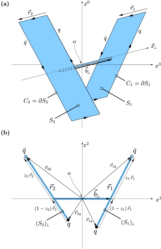
Figure 4.1: High-energy dipole-dipole scattering in the eikonal approximation represented by Wegner-Wilson loops in the fundamental representation of $SU(N_{c})$: (a) Space-time and (b) transverse arrangement of the Wegner-Wilson loops. The shaded areas represent the strings extending from the quark to the antiquark path in each color dipole. The thin tube allows us to compare the gluon field strengths in surface $S_{1}$ with the gluon field strengths in surface $S_{2}$. The impact parameter $\vec{b}_{\perp}$ connects the centers of light-cone momenta of the dipoles.

The dipole trajectories $C_{i}$ defining the Wegner-Wilson loops in (4.2) are described as straight lines. This is a good approximation as long as the kinematical assumption behind the eikonal approximation, $s\gg-t$, holds that allows us to neglect the change of the dipole velocities $v_{i}=p_{i}/m$ in the scattering process, where $p_{i}$ is the momentum and $m$ the mass of the considered dipole. Moreover, the paths $C_{i}$ are considered light-like in line with the high-energy limit, $m^{2}\ll s\to\infty$. For the hyperbolic angle or rapidity gap between the dipole trajectories $\gamma=(v_{1}\cdot v_{2})$ – which is the central quantity in the analytic continuation discussed below and also defined through $s=4m^{2}\cosh^{2}(\gamma/2)$ – the high-energy limit implies

$$\lim_{m^{2}\ll s\to\infty}\gamma\approx\ln(s/m^{2})\to\infty\ .$$ (4.4)

The QCD VEVs $\langle\ldots\rangle_{M}$ in the $S$-matrix element (4.2) represent Minkowskian functional integrals [34] in which – as in the Euclidean case discussed above – the functional integration over the fermion fields has already been carried out.

The $S$-matrix element $S^{M}_{DD}:=S^{M}_{\mbox{\scriptsize N}_{c}\mbox{\scriptsize N}_{c}}$ for the scattering of light-like dipoles in the fundamental $SU(N_{c}\!=\!3)$ representation ($r_{1}\!=\!r_{2}\!=\!\mbox{N}_{c}\!=\!3$) is the key to our unified description of hadron-hadron, photon-hadron, and photon-photon reactions in the following chapters. With color dipoles given by the quark and antiquark in the meson or photon or in a simplified picture by a quark and diquark in the baryon, we describe hadrons and photons as quark-antiquark or quark-diquark systems, i.e. fundamental $SU(3)$ dipoles, with size and orientation determined by appropriate light-cone wave functions [31, 32]. Accordingly, the $T$-matrix element for the reaction $ab\to cd$ factorizes into the universal $S$-matrix element $S^{M}_{DD}$ and reaction-specific light-cone wave functions $\psi_{a,b}$ and $\psi_{c,d}$ that describe the ${\vec{r}}_{i}$ and $z_{i}$ distribution of the color dipoles [31, 32, 34]

$$T_{ab\rightarrow cd}(s,t)=2is\int\!\!d^{2}b_{\!\perp}e^{i{\vec{q}}_{\!\perp}{\vec{b}}_{\!\perp}}\int\!\!dz_{1}d^{2}r_{1}\!\int\!\!dz_{2}d^{2}r_{2}\hphantom{\hskip 142.26378pt}$$

$$\!\!\times\!\! \psi_{c}^{*}(z_{1},\vec{r}_{1\perp})\,\psi_{d}^{*}(z_{2},\vec{r}_{2\perp})\left[1-S^{M}_{DD}(s,{\vec{b}}_{\!\perp},z_{1},\vec{r}_{1\perp},z_{2},\vec{r}_{2\perp})\right]\psi_{a}(z_{1},\vec{r}_{1\perp})\,\psi_{b}(z_{2},\vec{r}_{2\perp})\ .$$

Concentrating in this work on reactions with $a=c$ and $b=d$, the squared wave functions $|\psi_{1}(z_{1},\vec{r}_{1\perp})|^{2}:=\psi_{c}^{*}(z_{1},\vec{r}_{1\perp})\,\psi_{a}(z_{1},\vec{r}_{1\perp})$ and $|\psi_{2}(z_{2},\vec{r}_{2\perp})|^{2}:=\psi_{d}^{*}(z_{2},\vec{r}_{2\perp})\,\psi_{b}(z_{2},\vec{r}_{2\perp})$ are needed. We use for hadrons the phenomenological Gaussian wave function [61, 106] and for photons the perturbatively derived wave function with running quark masses $m_{f}(Q^{2})$ to account for the non-perturbative region of low photon virtuality $Q^{2}$ [52]. In Sec. 5.1 we specify and discuss these wave functions explicitly. The scattering of dipoles with fixed size $|\vec{r}_{i}|$ and fixed longitudinal quark momentum fraction $z_{i}$ averaged over all orientations,

$$|\psi_{\!\mbox{\tiny\it D}_{i}}(z_{i},\vec{r}_{i})|^{2}=\frac{1}{2\pi|\vec{r}_{\!\mbox{\tiny\it D}_{i}}|}\,\delta(|\vec{r}_{i}|-|\vec{r}_{\!\mbox{\tiny\it D}_{i}}|)\,\delta(z_{i}-z_{\!\mbox{\tiny\it D}_{i}})\ ,$$ (4.6)

is considered in Sec. 6.1 to show that $S$-matrix unitarity constraints are respected in our model. For the analytic continuation of high-energy scattering to Euclidean space-time, we now return to the scattering of dipoles with fixed size and orientation $\vec{r}_{i}$ and fixed longitudinal quark momentum fraction $z_{i}$.

4.2 Analytic Continuation of Dipole-Dipole Scattering

The Euclidean approach to the described elastic scattering of dipoles in the eikonal approximation is based on Meggiolaro’s analytic continuation of the high-energy parton-parton scattering amplitude [45]. Meggiolaro’s analytic continuation has been derived in the functional integral approach to high-energy collisions [33, 34] in which parton-parton scattering is described in terms of Wegner-Wilson lines: The Minkowskian amplitude, $g^{M}(\gamma,T,t)$, given by the expectation value of two Wegner-Wilson lines, forming an hyperbolic angle $\gamma$ in Minkowski space-time, and the Euclidean “amplitude,” $g^{E}(\Theta,T,t)$, given by the expectation value of two Wegner-Wilson lines, forming an angle $\Theta\in[0,\pi]$ in Euclidean space-time, are connected by the following analytic continuation in the angular variables and the temporal extension $T$, which is needed as an IR regulator in the case of Wegner-Wilson lines,

$$g^{E}(\Theta,T,t) = g^{M}(\gamma\to i\Theta,T\to-iT,t)\ ,$$ (4.7)

$$g^{M}(\gamma,T,t) = g^{E}(\Theta\to-i\gamma,T\to iT,t)\ .$$ (4.8)

Generalizing this relation to gauge-invariant dipole-dipole scattering described in terms of Wegner-Wilson loops [31, 32, 34], the IR divergence known from the case of Wegner-Wilson lines vanishes and no finite IR regulator $T$ is necessary. Thus, the Minkowskian $S$-matrix element (4.2), given by the expectation values of two Wegner-Wilson loops, forming an hyperbolic angle $\gamma$ in Minkowski space-time, can be computed from the Euclidean “$S$-matrix element”

$$S^{E}_{r_{1}r_{2}}(\Theta,{\vec{b}}_{\!\perp},z_{1},\vec{r}_{1\perp},z_{2},\vec{r}_{2\perp})=\lim_{T\rightarrow\infty}\frac{\langle W_{r_{1}}[C_{1}]W_{r_{2}}[C_{2}]\rangle_{E}}{\langle W_{r_{1}}[C_{1}]\rangle_{E}\langle W_{r_{2}}[C_{2}]\rangle_{E}}$$ (4.9)

given by the expectation values of two Wegner-Wilson loops, forming an angle $\Theta\in[0,\pi]$ in Euclidean space-time, via an analytic continuation in the angular variable

$$S^{M}_{r_{1}r_{2}}(\gamma\approx\ln[s/m^{2}],{\vec{b}}_{\!\perp},z_{1},\vec{r}_{1\perp},z_{2},\vec{r}_{2\perp})=S^{E}_{r_{1}r_{2}}(\Theta\to-i\gamma,{\vec{b}}_{\!\perp},z_{1},\vec{r}_{1\perp},z_{2},\vec{r}_{2\perp})\ ,$$ (4.10)

where $E$ indicates Euclidean space-time and the QCD VEVs $\langle\ldots\rangle_{E}$ represent Euclidean functional integrals that are equivalent to the ones denoted by $\langle\ldots\rangle_{G}$ in the preceding sections, i.e. in which the functional integration over the fermion fields has already been carried out.

The angle $\Theta$ is best illustrated in the relation of the Euclidean $S$-matrix element (4.9) to the van der Waals potential between two static dipoles $V_{r_{1}r_{2}}(\Theta=0,\vec{b},z_{1},\vec{r}_{1},z_{2},\vec{r}_{2})$, discussed in Sec. 4.4,

$$S^{E}_{r_{1}r_{2}}(\Theta,\vec{b}_{\!\perp},z_{1},\vec{r}_{1\perp},z_{2},\vec{r}_{2\perp})=\lim_{T\rightarrow\infty}\exp\!\left[-\,T\,V_{r_{1}r_{2}}(\Theta,\vec{b}_{\!\perp},z_{1},\vec{r}_{1\perp},z_{2},\vec{r}_{2\perp})\right]\ .$$ (4.11)

Figure 4.2 shows the loop-loop geometry necessary to compute $S^{E}_{r_{1}r_{2}}(\Theta\neq 0,\cdots)$ and how it is obtained by generalizing the geometry relevant for the computation of the potential between two static dipoles ($\Theta=0$): While the potential between two static dipoles is computed from two loops along parallel “temporal” unit vectors, $t_{1}=t_{2}=(0,0,0,1)$, the Euclidean $S$-matrix element (4.9) involves the tilting of one of the two loops, e.g. the tilting of $t_{1}$ by the angle $\Theta$ towards the $X_{3}$ - axis, $t_{1}=(0,0,-\sin\Theta,\cos\Theta)$. The “temporal” unit vectors $t_{i}$ are also discussed in Appendix A together with another illustration of the tilting angle $\Theta$.

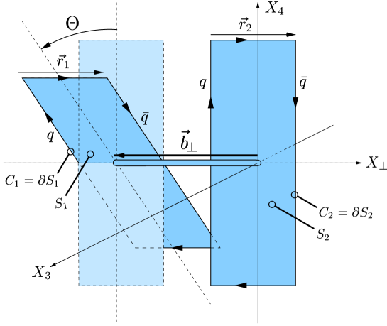
Figure 4.2: The loop-loop geometry necessary to compute $S^{E}_{r_{1}r_{2}}(\Theta\neq 0,\cdots)$ illustrated as a generalization of the geometry relevant for the computation of the van der Waals potential between two static dipoles ($\Theta=0$). While the potential between two static dipoles is computed from two loops along parallel “temporal” unit vectors, $t_{1}=t_{2}=(0,0,0,1)$, the Euclidean $S$-matrix element (4.9) involves the tilting of one of the two loops, e.g. the tilting of $t_{1}$ by the angle $\Theta$ towards the $X_{3}$ - axis, $t_{1}=(0,0,-\sin\Theta,\cos\Theta)$.

Since the Euclidean $S$-matrix element (4.9) involves only configurations of Wegner-Wilson loops in Euclidean space-time and Euclidean functional integrals, it can be computed directly on a Euclidean lattice. First attempts in this direction have been carried out but only very few signals could be extracted, while most of the data was dominated by noise [49]. Once precise results are available, the analytic continuation (4.10) will allow us to access hadronic high-energy reactions directly in lattice QCD, i.e. within a non-perturbative description of QCD from first principles. More generally, the presented gauge-invariant analytic continuation (4.10) makes any approach limited to a Euclidean formulation of the theory applicable for investigations of high-energy reactions. Indeed, Meggiorlaro’s analytic continuation has already been used to access high-energy scattering from the supergravity side of the AdS/CFT correspondence [46], which requires a positive definite metric in the definition of the minimal surface [47], and to examine the effect of instantons on high-energy scattering [48].

4.3 Dipole-Dipole Scattering in the LLCM

Let us now perform the analytic continuation explicitly in our Euclidean loop-loop correlation model. For the scattering of two color dipoles in the fundamental representation of $SU(N_{c})$, the Euclidean $S$-matrix element becomes with the VEVs (2.14) and (2.35)

$$S^{E}_{DD}(\Theta,\vec{b}_{\!\perp},z_{1},\vec{r}_{1\perp},z_{2},\vec{r}_{2\perp}) \!\!\!\!\!\!:=\,\,S^{E}_{\mbox{\scriptsize N}_{c}\mbox{\scriptsize N}_{c}}(\Theta,\vec{b}_{\!\perp},z_{1},\vec{r}_{1\perp},z_{2},\vec{r}_{2\perp})$$ (4.12)

$$=\lim_{T\rightarrow\infty}\left(\frac{N_{c}\!+\!1}{2N_{c}}\exp\!\left[-\frac{N_{c}\!-\!1}{2N_{c}}\chi_{S_{1}S_{2}}\right]+\frac{N_{c}\!-\!1}{2N_{c}}\exp\!\left[\frac{N_{c}\!+\!1}{2N_{c}}\chi_{S_{1}S_{2}}\right]\right)\ ,$$

where $\chi_{S_{i}S_{j}}$ – defined in (2.27) – decomposes into a perturbative ($P$) and non-perturbative ($N\!P$) component according to our decomposition of the gluon field strength correlator (2.42),

$$\chi_{S_{1}S_{2}}\,\,=\,\,\chi_{S_{1}S_{1}}^{P}\,+\,\chi_{S_{1}S_{2}}^{N\!P}\,\,=\,\,\chi_{S_{1}S_{2}}^{P}\,+\,\left(\chi_{S_{1}S_{2}}^{N\!P\,\,nc}\,+\,\chi_{S_{1}S_{2}}^{N\!P\,\,c}\right)\ .$$ (4.13)

In the limit $T_{1}=T_{2}=T\to\infty$ and for $\Theta\in[0,\pi]$, the components read

$$\chi_{S_{1}S_{2}}^{P}=\cot\Theta\,\,\chi^{P}\,\,,\quad\chi_{S_{1}S_{2}}^{N\!P\,\,nc}=\cot\Theta\,\,\chi^{N\!P\,\,nc}\,\,,\quad\chi_{S_{i}S_{j}}^{N\!P\,\,c}=\cot\Theta\,\,\chi^{N\!P\,\,c}$$ (4.14)

with

$$\!\!\!\!\!\!\!\!\!\!\!\!\!\chi^{P} \!\!=\!\! \left[g^{2}D^{\prime\,(2)}_{P}\left(|\vec{r}_{1q}-\vec{r}_{2{\bar{q}}}|\right)+g^{2}D^{\prime\,(2)}_{P}\left(|\vec{r}_{1{\bar{q}}}-\vec{r}_{2q}|\right)\right.$$ (4.15)

$$\left.-\,g^{2}D^{\prime\,(2)}_{P}\left(|\vec{r}_{1q}-\vec{r}_{2q}|\right)-g^{2}D^{\prime\,(2)}_{P}\left(|\vec{r}_{1{\bar{q}}}-\vec{r}_{2{\bar{q}}}|\right)\right]$$

$$\!\!\!\!\!\!\!\!\!\chi^{N\!P\,\,nc} \!\!=\!\! \frac{\pi^{2}G_{2}(1-\kappa)}{3(N_{c}^{2}-1)}\left[D^{\prime\,(2)}_{1}\left(|\vec{r}_{1q}-\vec{r}_{2{\bar{q}}}|\right)+D^{\prime\,(2)}_{1}\left(|\vec{r}_{1{\bar{q}}}-\vec{r}_{2q}|\right)\right.$$ (4.16)

$$\hphantom{-\frac{\pi^{2}G_{2}(1-\kappa)}{3(N_{c}^{2}-1)}}\left.-\,D^{\prime\,(2)}_{1}\left(|\vec{r}_{1q}-\vec{r}_{2q}|\right)-D^{\prime\,(2)}_{1}\left(|\vec{r}_{1{\bar{q}}}-\vec{r}_{2{\bar{q}}}|\right)\right]$$

$$\!\!\!\!\!\!\!\!\!\!\!\!\!\chi^{N\!P\,\,c} \!\!=\!\! \frac{\pi^{2}G_{2}\kappa}{3(N_{c}^{2}-1)}\,\left(\vec{r}_{1}\cdot\vec{r}_{2}\right)\int_{0}^{1}\!dv_{1}\int_{0}^{1}\!dv_{2}\,\,D^{(2)}\left(|\vec{r}_{1q}\!+\!v_{1}\vec{r}_{1\perp}\!-\!\vec{r}_{2q}\!-\!v_{2}\vec{r}_{2\perp}|\right)$$ (4.17)

as derived explicitly in Appendix B with the minimal surfaces illustrated in Fig. 4.2. In Eq. (4.15) the shorthand notation $g^{2}D^{\prime\,(2)}_{P}(|\vec{Z_{\perp}}|)=g^{2}(|\vec{Z_{\perp}}|)\,D^{\prime\,(2)}_{P}(|\vec{Z_{\perp}}|)$ is used with $g^{2}(|\vec{Z_{\perp}}|)$ again understood as the running coupling (2.47). The transverse Euclidean correlation functions

$$D_{x}^{(2)}(\vec{Z}^{2}):=\int\frac{d^{4}K}{(2\pi)^{2}}\,e^{iKZ}\,\tilde{D}_{x}(K^{2})\,\delta(K_{3})\,\delta(K_{4})$$ (4.18)

are obtained from the (massive) gluon propagator (2.43) and the exponential correlation function (2.50)

$$\!\!\!\!\!\!\!\!\!\!\!\!\!\!\!\!D^{\prime\,(2)}_{P}(\vec{Z}_{\!\perp}^{2}) \!\!=\!\! \frac{1}{2\pi}K_{0}\left(m_{G}|\vec{Z}_{\!\perp}|\right)$$ (4.19)

$$\!\!\!\!\!\!\!\!\!\!\!\!\!\!\!\!D^{\prime\,(2)}_{1}(\vec{Z}_{\!\perp}^{2}) \!\!=\!\! \pi a^{4}\Big{(}3\!+\!3\frac{|\vec{Z}_{\!\perp}|}{a}\!+\!\frac{|\vec{Z}_{\!\perp}|^{2}}{a^{2}}\Big{)}\exp\!\Big{(}\!-\frac{|\vec{Z}_{\!\perp}|}{a}\Big{)}$$ (4.20)

$$\!\!\!\!\!\!\!\!\!\!\!\!\!\!\!\!D^{(2)}(\vec{Z}_{\!\perp}^{2}) \!\!=\!\! 2\pi a^{2}\Big{(}1\!+\!\frac{|\vec{Z}_{\!\perp}|}{a}\Big{)}\exp\!\Big{(}\!-\frac{|\vec{Z}_{\!\perp}|}{a}\Big{)}$$ (4.21)

With the full $\Theta$-dependence exposed in (4.14), the analytic continuation (4.10) reads

$$\chi_{S_{1}S_{2}}=\cot\Theta\,\,\chi\quad\underrightarrow{\,\,\Theta\to-i\gamma\,\,\,\,}\quad\cot(-i\gamma)\,\chi\quad\underrightarrow{\,\,s\to\infty\,\,\,\,}\quad i\chi$$ (4.22)

and leads to the desired Minkowskian $S$-matrix element for elastic dipole-dipole scattering ($DD$) in the high-energy limit in which the dipoles move on the light-cone

$$\lim_{s\rightarrow\infty}S_{DD}^{M}(s,{\vec{b}}_{\!\perp},z_{1},\vec{r}_{1\perp},z_{2},\vec{r}_{2\perp}) \!\!\!\!\!\!:=\,\,\lim_{s\rightarrow\infty}S^{M}_{\mbox{\scriptsize N}_{c}\mbox{\scriptsize N}_{c}}(s,{\vec{b}}_{\!\perp},z_{1},\vec{r}_{1\perp},z_{2},\vec{r}_{2\perp})$$ (4.23)

$$=S^{E}_{DD}(\cot\Theta\to i,{\vec{b}}_{\!\perp},z_{1},\vec{r}_{1\perp},z_{2},\vec{r}_{2\perp})$$

$$=\lim_{T\rightarrow\infty}\left(\frac{N_{c}\!+\!1}{2N_{c}}\exp\!\left[-i\frac{N_{c}\!-\!1}{2N_{c}}\chi\right]+\frac{N_{c}\!-\!1}{2N_{c}}\exp\!\left[i\frac{N_{c}\!+\!1}{2N_{c}}\chi\right]\right)$$

where $\chi=\chi^{P}+\chi^{N\!P\,\,nc}+\chi^{N\!P\,\,c}$ with (4.15), (4.16), and (4.17).

It is striking that exactly the same result has been obtained in [23] with the alternative analytic continuation introduced for applications of the SVM to high-energy reactions [30, 31, 32]. In this complementary approach the gauge-invariant bilocal gluon field strength correlator is analytically continued from Euclidean to Minkowskian space-time by the substitution $\delta_{\mu\rho}\rightarrow-g_{\mu\rho}$ and the analytic continuation of the Euclidean correlation functions to real time $D^{E}_{x}(Z^{2})\rightarrow D^{M}_{x}(z^{2})$. In the subsequent steps, one finds $\langle W[C]\rangle_{M}=1$ due to the light-likeness of the loops and that the longitudinal correlations can be integrated out $\langle W_{r_{1}}[C_{1}]W_{r_{2}}[C_{2}]\rangle_{M}=f(s,{\vec{b}}_{\!\perp},\cdots)$. One is left with exactly the Euclidean correlations in transverse space that have been obtained above. This confirms the analytic continuation used in the earlier LLCM investigations in Minkowski space-time [23, 25, 24, 26] and in all earlier SVM applications to high-energy scattering [30, 31, 32, 50, 51, 52, 53, 54, 55, 56, 57, 58].

In the limit of small $\chi$-functions, $|\chi^{P}|\ll 1$ and $|\chi^{N\!P}|\ll 1$, (4.23) reduces to

$$\lim_{s\rightarrow\infty}S_{DD}^{M}(s,{\vec{b}}_{\!\perp},z_{1},\vec{r}_{1\perp},z_{2},\vec{r}_{2\perp})\approx 1+\frac{N_{c}^{2}-1}{8N_{c}^{2}}\,\chi^{2}=1+\frac{C_{2}(\mbox{N}_{c})}{4N_{c}}\,\chi^{2}\ .$$ (4.24)

The perturbative correlations, $(\chi^{P})^{2}$, describe the well-known two-gluon exchange contribution [99, 100] to dipole-dipole scattering, which is, of course, an important successful cross-check of the presented Euclidean approach to high-energy scattering. The non-perturbative correlations, $(\chi^{N\!P})^{2}$, describe the corresponding non-perturbative two-point interactions that contain contributions of the confining QCD strings to dipole-dipole scattering. We have analyzed these string contributions systematically as manifestations of confinement in high-energy scattering reactions and have indeed found a new characteristic structure (different from the perturbative dipole factors) in momentum space [24]. This analysis has also shown explicitly that the non-perturbative contribution governs – as expected – the region of low transverse momenta $|\vec{k}_{\!\perp}|$. Here, we focus on the structure in space-time representation and refer the reader for complementary insights to our momentum-space analysis [24].

As evident from the $v_{1}$ and $v_{2}$ integrations in (4.17) and Fig. 4.1b, there are contributions from the transverse projections of the minimal surfaces $(S_{1,2})_{\!\perp}$ connecting the quark and antiquark in each of the two dipoles. These are the contributions that we interpret as manifestations of the strings confining the quark and antiquark in each dipole. We thus understand the confining component $\chi_{c}^{N\!P}$ as a string-string interaction. Interestingly, we have found in dipole-hadron and dipole-photon interactions that the strings confining the quark-antiquark pair in the dipole can represented as an integral over stringless dipoles with a given dipole number density. As already mentioned, this decomposition of the confining string into dipoles even allows us to compute unintegrated gluon distributions of hadrons and photons and thus gives new insights into the microscopic structure of the non-perturbative SVM [24].

Both non-perturbative components, $\chi^{N\!P}_{c}$ and $\chi^{N\!P}_{nc}$, show color transparency for small dipoles, i.e. a dipole-dipole cross section with $\sigma_{DD}(\vec{r}_{1},\vec{r}_{2})\propto|\vec{r}_{1}|^{2}|\vec{r}_{2}|^{2}$ for $|\vec{r}_{1,2}|\to 0$, as known for the perturbative case [101]. This can be seen by squaring (4.16) and (4.17) to obtain the leading terms in the $T$-matrix element for small dipoles; see (4.24).

Due to the truncation of the cumulant expansion in the Gaussian approximation, a considerable dependence of $\chi_{c}^{N\!P}$ on the specific surface choice is observed. In fact, a different and more complicated result for $\chi_{c}^{N\!P}$ was obtained with the pyramid mantle choice for the surfaces $S_{1,2}$ in earlier applications of the SVM to high-energy scattering [31, 32, 50, 51, 52, 53, 54, 55, 56, 57, 61]. However, we use minimal surfaces in line with our model applications in Euclidean space-time discussed in the previous chapter. Moreover, the simplicity of the minimal surfaces allows us to give an analytic expression for the leading term of the non-perturbative dipole-dipole cross section [24]. Phenomenologically, in comparison with pyramid mantles, the description of the slope parameter $B(s)$, the differential elastic cross section $d\sigma^{el}/dt(s,t)$, and the elastic cross section $\sigma^{el}(s)$ can be improved with minimal surfaces as shown in Chap. 7. In contrast to the confining component $\chi_{c}^{N\!P}$, the non-confining components, $\chi_{nc}^{N\!P}$ and $\chi^{P}$, depend only on the transverse position between the quark and antiquark of the two dipoles and are therefore independent of the surface choice.

With the insights from the small-$\chi$ limit, one sees clearly that the full $S$-matrix element (4.23) describes multiple gluonic interactions. Indeed, the higher order terms in the expansion of the exponential functions in (4.23) are crucial to respect $S$-matrix unitarity constraints in impact parameter space [57, 23] as shown explicitly in Chap. 6.

Concerning the energy dependence, the $S$-matrix element (4.23) leads to energy-independent cross sections in contradiction to the experimental observation. Although disappointing from the phenomenological point of view, this is not surprising since our approach does not describe explicit gluon radiation needed for a non-trivial energy dependence. However, based on the $S$-matrix element (4.23), a phenomenological energy dependence can be constructed – see Sec. 5.2 – that allows a unified description of high-energy hadron-hadron, photon-hadron, and photon-photon reactions and an investigation of saturation effects in hadronic cross sections manifesting $S$-matrix unitarity [23, 25, 26]. This, of course, can only be an intermediate step. For a more fundamental understanding of hadronic high-energy reactions in our model, gluon radiation and quantum evolution have to be implemented explicitly.

Note that $\chi=\chi_{c}^{N\!P}+\chi_{nc}^{N\!P}+\chi^{P}$ is a real-valued function. Since, in addition, the wave functions $|\psi_{i}(z_{i},\vec{r}_{i\perp})|^{2}$ used in this work – see Sec. 5.1 – are invariant under the replacement $(\vec{r}_{i\perp}\rightarrow-\vec{r}_{i\perp},z_{i}\rightarrow 1-z_{i})$, the $T$-matrix element (4.1) with $S^{M}_{DD}$ given in (4.23) becomes purely imaginary and reads for $N_{c}=3$

$$\!\!\!\!\!\!\!\!\!\!\!\!\!T(s,t) = 2is\int\!\!d^{2}b_{\!\perp}e^{i{\vec{q}}_{\!\perp}{\vec{b}}_{\!\perp}}\int\!\!dz_{1}d^{2}r_{1}\!\int\!\!dz_{2}d^{2}r_{2}\,\,|\psi_{1}(z_{1},\vec{r}_{1\perp})|^{2}\,\,|\psi_{2}(z_{2},\vec{r}_{2\perp})|^{2}$$

$$\!\!\!\!\!\!\!\!\!\!\times\left[1-\frac{2}{3}\cos\!\left(\frac{1}{3}\chi({\vec{b}}_{\!\perp},z_{1},\vec{r}_{1\perp},z_{2},\vec{r}_{2\perp})\!\right)-\frac{1}{3}\cos\!\left(\frac{2}{3}\chi({\vec{b}}_{\!\perp},z_{1},\vec{r}_{1\perp},z_{2},\vec{r}_{2\perp})\!\right)\right].$$

The real part averages out in the integration over ${\vec{r}}_{i}$ and $z_{i}$ because of

$$\chi(\vec{b}_{\!\perp},1-z_{1},-\vec{r}_{1\perp},z_{2},\vec{r}_{2\perp})=-\chi(\vec{b}_{\!\perp},z_{1},\vec{r}_{1\perp},z_{2},\vec{r}_{2\perp})\ ,$$ (4.26)

which can be seen directly from (4.15),(4.16), and (4.17) as $(\vec{r}_{1\perp}\rightarrow-\vec{r}_{1\perp},z_{1}\rightarrow 1-z_{1})$ implies $\vec{r}_{1q}\rightarrow\vec{r}_{1{\bar{q}}}$. In physical terms, $(\vec{r}_{i\perp}\rightarrow-\vec{r}_{i\perp},z_{i}\rightarrow 1-z_{i})$ corresponds to charge conjugation, i.e. the replacement of each parton with its antiparton and the associated reversal of the loop direction. Consequently, the $T$-matrix (4.3) describes only charge conjugation $C=+1$ exchange. Since in our quenched approximation purely gluonic interactions are modeled, (4.3) describes only pomeron but not reggeon exchange.

Although the scattering of two color dipoles in the fundamental representation of $SU(N_{c})$ is the most relevant case, we can derive immediately also the Minkowskian $S$-matrix element for the scattering of a fundamental ($D$) and an adjoint dipole (“glueball” $G\!B$) in the Euclidean LLCM. Using (2.40) and proceeding otherwise as above, we find in the high-energy limit

$$\!\!\!\!\!\!\!\!\lim_{s\rightarrow\infty}S^{M}_{D\,G\!B}(s,\vec{b},z_{1},\vec{r}_{1\perp},z_{2},\vec{r}_{2\perp})\,\,:=\,\,\lim_{s\rightarrow\infty}S^{M}_{\mbox{\scriptsize N}_{c}\,\mbox{\scriptsize N}_{c}^{2}\!-\!1}(\Theta,\vec{b},z_{1},\vec{r}_{1\perp},z_{2},\vec{r}_{2\perp})$$ (4.27)

$$\!\!\!\!\!\!\!\!=\lim_{T\rightarrow\infty}\Bigg{(}\,\frac{1}{N_{c}^{2}\!-\!1}\,\exp\!\Big{[}i\,\frac{N_{c}}{2}\,\chi\Big{]}+\frac{N_{c}\!+\!2}{2(N_{c}\!+\!1)}\exp\!\Big{[}\!-\,i\,\frac{1}{2}\,\chi\Big{]}+\frac{N_{c}\!-\!2}{2(N_{c}\!-\!1)}\exp\!\Big{[}i\,\frac{1}{2}\,\chi\Big{]}\Bigg{)}\ .$$

where $\chi=\chi^{P}+\chi^{N\!P\,nc}+\chi^{N\!P\,c}$ with (4.15), (4.16), and (4.17).

4.4 Comments on the QCD van der Waals Potential

Finally, we would like to comment on the QCD van der Waals interaction between two color dipoles, which is – as mentioned together with (4.11) – related to the Euclidean $S$-matrix element in the limiting case of $\Theta=0$: The QCD van der Waals potential between two static dipoles reads in terms of Wegner-Wilson loops [102, 103]

$$V_{r_{1}r_{2}}(\Theta=0,\vec{b},z_{1}=1/2,\vec{r}_{1},z_{2}=1/2,\vec{r}_{2})=-\lim_{T\rightarrow\infty}\frac{1}{T}\ln\frac{\langle W_{r_{1}}[C_{1}]W_{r_{2}}[C_{2}]\rangle}{\langle W_{r_{1}}[C_{1}]\rangle\langle W_{r_{2}}[C_{2}]\rangle}\ .$$ (4.28)

In this limit ($\Theta=0$) intermediate octet states and their limited lifetime become important as is well known from perturbative computations of the QCD van der Waals potential between two static color dipoles [102, 103, 104]: Working with static dipoles, i.e. infinitely heavy color sources, there is an energy degeneracy between the intermediate octet states and the initial (final) singlet states that leads for perturbative two-gluon exchange to a linear divergence in $T$ as $T\to\infty$. This IR divergence can be lifted by introducing manually an energy gap between the singlet ground state and the excited octet state and thus a limit on the lifetime of the intermediate octet state [102, 103, 104].

In the perturbative limit of $g^{2}\to 0$ and $T$ large but finite, i.e. $\chi^{P}\ll 1$, the perturbative component of our model describes the two-gluon exchange contribution to the van der Waals potential which is plagued by the discussed IR divergence resulting from the static limit. In the more general case of $g^{2}$ finite and $T\to\infty$, which does not exclude non-perturbative physics, one cannot use the small-$\chi$ limit and multiple gluonic interactions become important. Here our perturbative component describes multiple gluon exchanges that reduce to an effective one-gluon exchange contribution to the van der Waals potential whose interaction range ($\propto 1/m_{G}$) contradicts the common expectations. Indeed, it is also in contradiction to our results for the glueball mass $M_{G\!B}$ which determines the interaction range ($\propto 1/M_{G\!B}$) between two color dipoles for large dipole separations. As already mentioned in Sec. 2.3, we find for the perturbative component, $M_{G\!B}^{P}=2m_{G}$, i.e. half of the interaction range of one-gluon exchange, by computing the exponential decay of the correlation of two small quadratic loops $P^{\alpha\beta}_{r_{i}}$ for large Euclidean times $\tau\to\infty$

$$M_{G\!B}:=-\lim_{\tau\rightarrow\infty}\frac{1}{\tau}\ln\frac{\langle P_{r_{1}}^{\alpha\beta}(0)P_{r_{2}}^{\alpha\beta}(\tau)\rangle}{\langle P_{r_{1}}^{\alpha\beta}(0)\rangle\langle P_{r_{2}}^{\alpha\beta}(\tau)\rangle}\ .$$ (4.29)

Note that we find for the non-perturbative component, $M_{G\!B}^{N\!P}=2/a$, which is smaller than $M_{G\!B}^{P}=2m_{G}$ with the LLCM parameters and thus governs the long range correlations in the LLCM.

Thus, for a meaningful investigation of the QCD van der Waals forces within our model, one has to go beyond the static limit in order to describe the limited lifetime of the intermediate octet states appropriately. This we postpone for future work since the focus in this work is on high-energy scattering where the gluons are always exchanged within a short time interval due to the light-likeness of the scattered particles and the finite correlation lengths. Nevertheless, going beyond the static limit in the dipole-dipole potential means going beyond the eikonal approximation in high-energy scattering and it is, of course, of utmost importance to see how such generalizations alter our results.

Chapter 5 Hadronic Wave Functions and Universal Energy Dependence

In this chapter hadron and photon wave functions are provided and a universal energy dependence is constructed. Together with the $T$-matrix element (4.3), these ingredients are crucial for our unified description of hadron-hadron, photon-hadron, and photon-photon reactions in the following chapters. The model parameters adjusted in fits to experimental data are summarized at the end of this chapter.

5.1 Hadron and Photon Wave Functions

The light-cone wave functions $\psi_{i}(z_{i},\vec{r}_{i})$ provide the distribution of transverse size and orientation ${\vec{r}}_{i}$ and longitudinal quark momentum fraction $z_{i}$ to the light-like Wegner-Wilson loops $W[C_{i}]$ that represent the scattering color dipoles. In this way, they specify the projectiles as mesons, baryons described as quark-diquark systems, or photons that fluctuate into a quark-antiquark pair before the interaction.

The Hadron Wave Function

In this work mesons and baryons are assumed to have a quark-antiquark and quark-diquark valence structure, respectively. As quark-diquark systems are equivalent to quark-antiquark systems [105], this allows us to model not only mesons but also baryons as color dipoles represented by Wegner-Wilson loops. To characterize mesons and baryons, we use the phenomenological Gaussian Wirbel-Stech-Bauer ansatz [106]

$$\psi_{h}(z_{i},\vec{r}_{i})=\sqrt{\frac{z_{i}(1-z_{i})}{2\pi S_{h}^{2}N_{h}}}\,e^{-(z_{i}-\frac{1}{2})^{2}/(4\Delta z_{h}^{2})}\,e^{-|\vec{r}_{i}|^{2}/(4S_{h}^{2})}\ ,$$ (5.1)

where the hadron wave function normalization to unity

$$\int\!\!dz_{i}d^{2}r_{i}\ |\psi_{i}(z_{i},\vec{r}_{i})|^{2}=1\ ,$$ (5.2)

requires the normalization constant

$$N_{h}=\int_{0}^{1}dz_{i}\ z_{i}(1-z_{i})\ e^{-(z_{i}-\frac{1}{2})^{2}/(2\Delta z_{h}^{2})}\ .$$ (5.3)

The different hadrons considered – protons, pions, and kaons – are specified by $\Delta z_{h}$ and $S_{h}$ providing the width for the distributions of the longitudinal momentum fraction carried by the quark $z_{i}$ and transverse spatial extension $|\vec{r}_{i}|$, respectively. In this work the extension parameter $S_{h}$ is a fit parameter that should resemble approximately the electromagnetic radius of the corresponding hadron [61], while $\Delta z_{h}=w/(\sqrt{2}\,m_{h})$ [106] is fixed by the hadron mass $m_{h}$ and the value $w=0.35-0.5\,\mbox{GeV}$ extracted from experimental data. We find for (anti-)protons $\Delta z_{p}=0.3$ and $S_{p}=0.86\,\mbox{fm}$, for pions $\Delta z_{\pi}=2$ and $S_{\pi}=0.607\,\mbox{fm}$, and for kaons $\Delta z_{K}=0.57$ and $S_{K}=0.55\,\mbox{fm}$ which are the values used in the main text. For convenience they are summarized in Table 5.1.

Table 5.1: Hadron Parameters

Hadron	$\Delta z_{h}$	$S_{h}\;[\mbox{fm}]$
$p,\bar{p}$	$0.3$	$0.86$
$\pi^{\pm}$	$2$	$0.607$
$K^{\pm}$	$0.57$	$0.55$

Concerning the quark-diquark structure of the baryons, the more conventional three-quark structure of a baryon would complicate the model significantly but would lead to similar predictions once the model parameters are readjusted [31]. In fact, there are also physical arguments that favor the quark-diquark structure of the baryon such as the $\delta I=1/2$ enhancement in semi-leptonic decays of baryons [105] and the strong attraction in the scalar diquark channel in the instanton vacuum [107].

The Photon Wave Function

The photon wave function $\psi_{\gamma}(z_{i},\vec{r}_{i},Q^{2})$ describes the fluctuation of a photon with virtuality $Q^{2}$ into a quark-antiquark pair with longitudinal quark momentum fraction $z_{i}$ and spatial transverse size and orientation $\vec{r}_{i}$. The computation of the corresponding transition amplitude $\langle q{\bar{q}}(z_{i},\vec{r}_{i})|\gamma^{*}(Q^{2})\rangle$ can be performed conveniently in light-cone perturbation theory [108] and leads to the following squared wave functions for transverse $(T)$ and longitudinally $(L)$ polarized photons [101]

$$\!\!\!\!\!\!\!\!\!\!\!\!\!|\psi_{\gamma_{T}^{*}}(z_{i},\vec{r}_{i},Q^{2})|^{2}\! \!\!=\!\! \!\frac{3\,\alpha}{2\,\pi^{2}}\sum_{f}e_{f}^{2}\left\{\left[z_{i}^{2}+(1-z_{i})^{2}\right]\,\epsilon_{f}^{2}\,K_{1}^{2}(\epsilon_{f}\,|\vec{r}_{i}|)+m_{f}^{2}\,K_{0}^{2}(\epsilon_{f}\,|\vec{r}_{i}|)\right\}$$ (5.4)

$$\!\!\!\!\!\!\!\!\!\!\!\!\!|\psi_{\gamma_{L}^{*}}(z_{i},\vec{r}_{i},Q^{2})|^{2}\! \!\!=\!\! \!\frac{3\,\alpha}{2\,\pi^{2}}\sum_{f}e_{f}^{2}\left\{4\,Q^{2}\,z_{i}^{2}(1-z_{i})^{2}\,K_{0}^{2}(\epsilon_{f}\,|\vec{r}_{i}|)\right\},$$ (5.5)

where $\alpha$ is the fine-structure constant, $e_{f}$ is the electric charge of the quark with flavor $f$, and $K_{0}$ and $K_{1}$ are the modified Bessel functions (McDonald functions). In the above expressions,

$$\epsilon_{f}^{2}=z_{i}(1-z_{i})\,Q^{2}+m_{f}^{2}$$ (5.6)

controlls the transverse size(-distribution) of the emerging dipole, $|\vec{r}_{i}|\propto 1/\epsilon_{f}$, that depends on the quark flavor through the current quark mass $m_{f}$.

For small $Q^{2}$, the perturbatively derived wave functions, (5.4) and (5.5), are not appropriate since the resulting color dipoles of size $|\vec{r}_{i}|\propto 1/m_{f}\gg 1\,\mbox{fm}$ should encounter non-perturbative effects such as confinement and chiral symmetry breaking. To take these effects into account the vector meson dominance (VMD) model [109] is usually used. However, the transition from the “partonic” behavior at large $Q^{2}$ to the “hadronic” one at small $Q^{2}$ can be modeled as well by introducing $Q^{2}$-dependent quark masses, $m_{f}=m_{f}(Q^{2})$, that interpolate between the current quarks at large $Q^{2}$ and the constituent quarks at small $Q^{2}$ [52]. Following this approach, we use (5.4) and (5.5) also in the low-$Q^{2}$ region but with the running quark masses

$$m_{u,d}(Q^{2}) = 0.178\,\mbox{GeV}\,(1-\frac{Q^{2}}{Q^{2}_{u,d}})\,\Theta(Q^{2}_{u,d}-Q^{2})\ ,$$ (5.7)

$$m_{s}(Q^{2}) = 0.121\,\mbox{GeV}+0.129\,\mbox{GeV}\,(1-\frac{Q^{2}}{Q^{2}_{s}})\,\Theta(Q^{2}_{s}-Q^{2})\ ,$$ (5.8)

and the fixed charm quark mass

$$m_{c}=1.25\,\mbox{GeV}\ ,$$ (5.9)

where the parameters $Q^{2}_{u,d}=1.05\,\mbox{GeV}^{2}$ and $Q^{2}_{s}=1.6\,\mbox{GeV}^{2}$ are taken directly from [52] while we reduced the values for the constituent quark masses $m_{f}(Q^{2}=0)$ of [52] by about 20%. The smaller constituent quark masses are necessary to reproduce the total cross sections for $\gamma^{*}p$ and $\gamma^{*}\gamma^{*}$ reactions at low $Q^{2}$. Similar running quark masses are obtained in a QCD-motivated model of spontaneous chiral symmetry breaking in the instanton vacuum [110] that improve the description of $\gamma^{*}p$ scattering at low $Q^{2}$ [111].

5.2 Universal Energy Dependence

Until now the $T$-matrix element (4.3) leads to energy independent total cross sections in contradiction to the experimental observation. In this section we introduce the energy dependence in a phenomenological way inspired by other successful models.

Most models for high-energy scattering are constructed to describe either hadron-hadron or photon-hadron reactions. For example, Kopeliovich et al. [112] as well as Berger and Nachtmann [57] focus on hadron-hadron scattering. In contrast, Golec-Biernat and Wüsthoff [113] and Forshaw, Kerley, and Shaw [114] concentrate on photon-proton reactions. A model that describes the energy dependence in both hadron-hadron and photon-hadron reactions up to large photon virtualities is the two-pomeron model of Donnachie and Landshoff [62]. Based on Regge theory [35], they find a soft pomeron trajectory with intercept $1+\epsilon_{\mathrm{soft}}\approx 1.08$ that governs the weak energy dependence of hadron-hadron or $\gamma^{*}p$ reactions with low $Q^{2}$ [115] and a hard pomeron trajectory with intercept $1+\epsilon_{\mathrm{hard}}\approx 1.4$ that governs the strong energy dependence of $\gamma^{*}p$ reactions with high $Q^{2}$ [62]. Similarly, we aim at a simultaneous description of hadron-hadron, photon-proton, and photon-photon reactions involving real and virtual photons as well.

In line with other two-component (soft $+$ hard) models [62, 114, 55, 56, 60] and the different hadronization mechanisms in soft and hard collisions, our physical ansatz demands that the perturbative and non-perturbative contributions do not interfere. Therefore, we modify the cosine-summation in (4.3) allowing only even numbers of soft and hard correlations, $\left(\chi^{N\!P}\right)^{2n}\left(\chi^{P}\right)^{2m}$ with $n,m\in I\!\!N$. Interference terms with odd numbers of soft and hard correlations are subtracted by the replacement

$$\cos\left[c\chi\right]=\cos\left[c\left(\chi^{N\!P}+\chi^{P}\right)\right]\rightarrow\cos\left[c\chi^{N\!P}\right]\cos\left[c\chi^{P}\right]\ ,$$ (5.10)

where $c=1/3$ or $2/3$. This prescription leads to the following factorization of soft and hard physics in the $T$-matrix element,

$$\!\!\!\!\!\!\!\!\!\!T(s,t)=2is\int\!\!d^{2}b_{\!\perp}e^{i{\vec{q}}_{\!\perp}{\vec{b}}_{\!\perp}}\int\!\!dz_{1}d^{2}r_{1}\!\int\!\!dz_{2}d^{2}r_{2}\,\,|\psi_{1}(z_{1},\vec{r}_{1})|^{2}\,\,|\psi_{2}(z_{2},\vec{r}_{2})|^{2}$$

$$\!\!\!\!\!\!\!\!\!\!\!\!\times\left[1-\frac{2}{3}\cos\!\left(\!\frac{1}{3}\chi^{N\!P}\!\right)\cos\!\left(\!\frac{1}{3}\chi^{P}\!\right)-\frac{1}{3}\cos\!\left(\!\frac{2}{3}\chi^{N\!P}\!\right)\cos\!\left(\!\frac{2}{3}\chi^{P}\!\right)\right]\ .$$ (5.11)

In the limit of small $\chi$-functions, $\chi^{N\!P}\ll 1$ and $\chi^{P}\ll 1$, one gets

$$T(s,t) = 2is\!\int\!\!d^{2}b_{\!\perp}e^{i{\vec{q}}_{\!\perp}{\vec{b}}_{\!\perp}}\!\int\!\!dz_{1}d^{2}r_{1}\!\int\!\!dz_{2}d^{2}r_{2}\,\,|\psi_{1}(z_{1},\vec{r}_{1})|^{2}\,\,|\psi_{2}(z_{2},\vec{r}_{2})|^{2}$$ (5.12)

$$\times\frac{1}{9}\left[\left(\chi^{N\!P}\right)^{2}+\left(\chi^{P}\right)^{2}\right]$$

so that the $T$-matrix element becomes a sum of a perturbative and a non-perturbative component. As already discussed in Sec. 4.3, the perturbative component $(\chi^{P})^{2}$ coincides with the well-known perturbative two-gluon exchange [99, 100] and the non-perturbative component $(\chi^{N\!P})^{2}$ represents the corresponding non-perturbative gluonic interaction on the “two-gluon-exchange” level [24].

As the two-component structure of (5.12) reminds of the two-pomeron model of Donnachie and Landshoff [62], we adopt the powerlike energy increase and ascribe a weak energy dependence to the non-perturbative component $\chi^{N\!P}$ and a strong one to the perturbative component $\chi^{P}$

$$\left(\chi^{N\!P}\right)^{2}\quad \rightarrow \quad\left(\chi^{N\!P}(s)\right)^{2}:=\left(\chi^{N\!P}\right)^{2}\left(\frac{s}{s_{0}}\frac{\vec{r}_{1}^{\,2}\,\vec{r}_{2}^{\,2}}{R_{0}^{4}}\right)^{\epsilon^{N\!P}}$$

$$\left(\chi^{P}\right)^{2}\quad \rightarrow \quad\left(\chi^{P}(s)\right)^{2}:=\left(\chi^{P}\right)^{2}\left(\frac{s}{s_{0}}\frac{\vec{r}_{1}^{\,2}\,\vec{r}_{2}^{\,2}}{R_{0}^{4}}\right)^{\epsilon^{P}}$$ (5.13)

with the scaling factor $s_{0}R_{0}^{4}$. The powerlike energy dependence with the exponents $0\approx\epsilon^{N\!P}<\epsilon^{P}<1$ guarantees Regge type behavior at moderately high energies, where the small-$\chi$ limit (5.12) is appropriate. In (5.13) the energy variable $s$ is scaled by the factor $\vec{r}_{1}^{\,2}\,\vec{r}_{2}^{\,2}$ that allows to rewrite the energy dependence in photon-hadron scattering in terms of the appropriate Bjorken scaling variable $x$

$$s\,\vec{r}_{1}^{\,2}\propto\frac{s}{Q^{2}}=\frac{1}{x}\ ,$$ (5.14)

where $|\vec{r}_{1}|$ is the transverse extension of the $q{\bar{q}}$ dipole in the photon. A similar factor has been used before in the dipole model of Forshaw, Kerley, and Shaw [114] and also in the model of Donnachie and Dosch [60] in order to respect the scaling properties observed in the structure function of the proton. In the dipole-proton cross section of Golec-Biernat and Wüsthoff [113], Bjorken $x$ is used directly as energy variable which is important for the success of the model. In fact, also in our model, the $\vec{r}_{1}^{\,2}\,\vec{r}_{2}^{\,2}$ factor improves the description of $\gamma^{*}p$ reactions at large $Q^{2}$.

The powerlike Regge type energy dependence introduced in (5.13) is, of course, not mandatory but allows successful fits and can also be derived in other theoretical frameworks: A powerlike energy dependence is found for hard photon-proton reactions from the BFKL equation [116] and for hadronic reactions by Kopeliovich et al. [112]. However, these approaches need unitarization since their powerlike energy dependence will ultimately violate $S$-matrix unitarity at asymptotic energies. In our model we use the following $T$-matrix element for investigations in the remaining chapters

$$\!\!\!\!\!\!\!\!\!\!T(s,t)=2is\int\!\!d^{2}b_{\!\perp}e^{i{\vec{q}}_{\!\perp}{\vec{b}}_{\!\perp}}\int\!\!dz_{1}d^{2}r_{1}\!\int\!\!dz_{2}d^{2}r_{2}\,\,|\psi_{1}(z_{1},\vec{r}_{1})|^{2}\,\,|\psi_{2}(z_{2},\vec{r}_{2})|^{2}$$ (5.15)

$$\!\!\!\!\!\!\!\!\!\!\!\!\times\left[1-\frac{2}{3}\cos\!\left(\!\frac{1}{3}\chi^{N\!P}(s)\!\right)\cos\!\left(\!\frac{1}{3}\chi^{P}(s)\!\right)-\frac{1}{3}\cos\!\left(\!\frac{2}{3}\chi^{N\!P}(s)\!\right)\cos\!\left(\!\frac{2}{3}\chi^{P}(s)\!\right)\right]\ ,$$

where the cosine functions ensure the unitarity condition in impact parameter space as shown in Chap. 6. Indeed, the multiple gluonic interactions associated with the higher order terms in the expansion of the cosine functions are important for the saturation effects observed within our model at ultra-high energies.

Having ascribed the energy dependence to the $\chi$-function, the energy behavior of hadron-hadron, photon-hadron, and photon-photon scattering results exclusively from the universal dipole-dipole scattering kernel.

5.3 Model Parameters for High-Energy Scattering

Lattice QCD simulations provide important information and constraints on the model parameters as discussed in Chap. 2. The fine tuning of the parameters was, however, directly performed on high-energy scattering data for hadron-hadron, photon-hadron, and photon-photon reactions [23] where an error ($\chi^{2}$) minimization was not feasible because of the non-trivial multi-dimensional integrals in the $T$-matrix element (5.15).

The parameters $a$, $\kappa$, $G_{2}$, $m_{G}$, $M^{2}$, $s_{0}R^{4}_{0}$, $\epsilon^{N\!P}$ and $\epsilon^{P}$ determine the dipole-dipole scattering amplitude and are universal for all reactions considered. In addition, there are reaction-dependent parameters in the wave functions which are given in Sec. 5.1.

The non-perturbative component involves the correlation length $a$, the gluon condensate $G_{2}$, and the parameter $\kappa$ indicating the non-Abelian character of the correlator. With the simple exponential correlation function (2.50), we obtain the values given in (2.51) that have already been applied in Chap. 3

$$a=0.302\,\mbox{fm},\quad\kappa=0.74,\quad G_{2}=0.074\,\mbox{GeV}^{4}\ .$$

The perturbative component involves the gluon mass $m_{G}$ as IR regulator (or inverse “perturbative correlation length”) and the parameter $M^{2}$ that freezes the running coupling (2.47) for large distance scales. The following values are used in the following investigations

$$m_{G}=m_{\rho}=0.77\,\mbox{GeV}\quad\mbox{and }\quad M^{2}=1.04\,\mbox{GeV}^{2}\ .$$ (5.16)

The energy dependence of the model is associated with the energy exponents $\epsilon^{N\!P}$ and $\epsilon^{P}$, and the scaling parameter $s_{0}R^{4}_{0}$

$$\epsilon^{N\!P}=0.125,\quad\epsilon^{P}=0.73,\quad\mbox{and}\quad s_{0}R_{0}^{4}=(\,47\,\mbox{GeV}\,\mbox{fm}^{2}\,)^{2}\ .$$ (5.17)

In comparison to the energy exponents of Donnachie and Landshoff [115, 62], $\epsilon_{\mathrm{soft}}\approx 0.08$ and $\epsilon_{\mathrm{hard}}\approx 0.4$, our exponents are significantly larger. However, the cosine functions in our $T$-matrix element (5.15) reduce the large exponents so that the energy dependence of the cross sections agrees with the experimental data as illustrated in Chap. 7.

Chapter 6 Impact Parameter Profiles and Gluon Saturation

In this chapter $S$-matrix unitarity constraints are considered in our model. On the basis of the impact parameter dependence of the scattering amplitude, saturation effects can be exposed that manifest the $S$-matrix unitarity. For each impact parameter the energy at which the unitarity limit becomes important can be determined. The results are used to discuss gluon saturation and to localize saturation effects in experimental observables.

The impact parameter dependence of the scattering amplitude is given by ${\cal T}(s,|\vec{b}_{\!\perp}|)$,

$$T(s,t=-{\vec{q}}_{\!\perp}^{\,\,2})\;=\;4s\!\int\!\!d^{2}b_{\!\perp}\,e^{i{\vec{q}}_{\!\perp}{\vec{b}}_{\!\perp}}\,{\cal T}(s,|\vec{b}_{\!\perp}|)\ ,$$ (6.1)

and in particular by the profile function

$$J(s,|\vec{b}_{\!\perp}|)=2\,\mbox{Im}{\cal T}(s,|\vec{b}_{\!\perp}|)\ ,$$ (6.2)

which describes the blackness or opacity of the interacting particles as a function of the impact parameter $|{\vec{b}}_{\!\perp}|$ and the c.m. energy $\sqrt{s}$. In fact, the profile function (6.2) determines all observables if the $T$-matrix is – as in our model – purely imaginary.

6.1 $S$-Matrix Unitarity Constraints

The $S$-matrix unitarity, $SS^{\dagger}=S^{\dagger}S={1\!\rm l}$, leads directly to the unitarity condition in impact parameter space [117, 118]

$$\mbox{Im}{\cal T}(s,|\vec{b}_{\!\perp}|)=|{\cal T}(s,|\vec{b}_{\!\perp}|)|^{2}+G_{inel}(s,|\vec{b}_{\!\perp}|)\ ,$$ (6.3)

where $G_{inel}(s,|\vec{b}_{\!\perp}|)\geq 0$ is the inelastic overlap function [119]. This unitarity condition imposes an absolute limit on the profile function

$$0\;\;\leq\;\;2\,|{\cal T}(s,|\vec{b}_{\!\perp}|)|^{2}\;\;\leq\;\;J(s,|\vec{b}_{\!\perp}|)\;\;\leq\;\;2$$ (6.4)

and the inelastic overlap function, $G_{inel}(s,|\vec{b}_{\!\perp}|)\leq 1/4$. At high energies, the elastic amplitude is expected to be purely imaginary. Consequently, the solution of (6.3) reads

$$J(s,|\vec{b}_{\!\perp}|)=1\pm\sqrt{1-4\,G_{inel}(s,|\vec{b}_{\!\perp}|)}$$ (6.5)

and leads with the minus sign corresponding to the physical situation to the reduced unitarity bound

$$0\;\;\leq\;\;J(s,|\vec{b}_{\!\perp}|)\;\;\leq\;\;1\ .$$ (6.6)

Reaching the black disc limit or maximum opacity at a certain impact parameter $|\vec{b}_{\!\perp}|$, $J(s,|\vec{b}_{\!\perp}|)=1$, corresponds to maximal inelastic absorption $G_{inel}(s,|\vec{b}_{\!\perp}|)=1/4$ and equal elastic and inelastic contributions to the total cross section at that impact parameter.

In our model every reaction is reduced to dipole-dipole scattering with well defined dipole sizes $|{\vec{r}}_{i}|$ and longitudinal quark momentum fractions $z_{i}$ as discussed in Sec. 4.1. Thus, the most general test of our model with respect to the unitarity constraints is performed with the profile function

$$J_{DD}(s,|\vec{b}_{\!\perp}|,z_{1},|\vec{r}_{1}|,z_{2},|\vec{r}_{2}|)=\int\frac{d\phi_{1}}{2\pi}\int\frac{d\phi_{2}}{2\pi}\left[1-S_{DD}(s,\vec{b}_{\!\perp},z_{1},{\vec{r}}_{1},z_{2},{\vec{r}}_{2})\right]\ ,$$ (6.7)

where $\phi_{i}$ describes the dipole orientation, i.e. the angle between ${\vec{r}}_{i}$ and $\vec{b}_{\!\perp}$, and $S_{DD}$ describes elastic dipole-dipole scattering

$$S_{DD}=\frac{2}{3}\cos\!\left(\frac{1}{3}\chi^{N\!P}(s)\right)\cos\!\left(\frac{1}{3}\chi^{P}(s)\right)+\frac{1}{3}\cos\!\left(\frac{2}{3}\chi^{N\!P}(s)\right)\cos\!\left(\frac{2}{3}\chi^{P}(s)\right)$$ (6.8)

with the purely real-valued eikonal functions $\chi^{N\!P}(s)$ and $\chi^{P}(s)$ defined in (5.13). Because of $|S_{DD}|\leq 1$, a consequence of the cosine functions in (6.8) describing multiple gluonic interactions, $J_{DD}$ respects the absolute limit (6.4). Thus, the elastic dipole-dipole scattering respects the unitarity condition (6.3). At high energies, the arguments of the cosine functions in $S_{DD}$ become so large that these cosines average to zero in the integration over the dipole orientations. This leads to the black disc limit $J_{DD}^{\mathrm{max}}=1$ reached at high energies first for small impact parameters.

6.2 The Profile Function for Proton-Proton Scattering

The profile function for proton-proton scattering

$$J_{pp}(s,|\vec{b}_{\!\perp}|)=\int\!\!dz_{1}d^{2}r_{1}\!\int\!\!dz_{2}d^{2}r_{2}|\psi_{p}(z_{1},\vec{r}_{1})|^{2}|\psi_{p}(z_{2},\vec{r}_{2})|^{2}\left[1-S_{DD}(s,\vec{b}_{\!\perp},z_{1},{\vec{r}}_{1},z_{2},{\vec{r}}_{2})\right]$$ (6.9)

is obtained from (6.7) by weighting the dipole sizes $|{\vec{r}}_{i}|$ and longitudinal quark momentum fractions $z_{i}$ with the proton wave function $|\psi_{p}(z_{i},\vec{r}_{i})|^{2}$ from Sec. 5.1.

Using the model parameters from Sec. 5.3, we obtain the profile function $J_{pp}(s,|\vec{b}_{\!\perp}|)$ shown in Fig. 6.1 for c.m. energies from $\sqrt{s}=10\,\mbox{GeV}$ to $10^{8}\,\mbox{GeV}$.

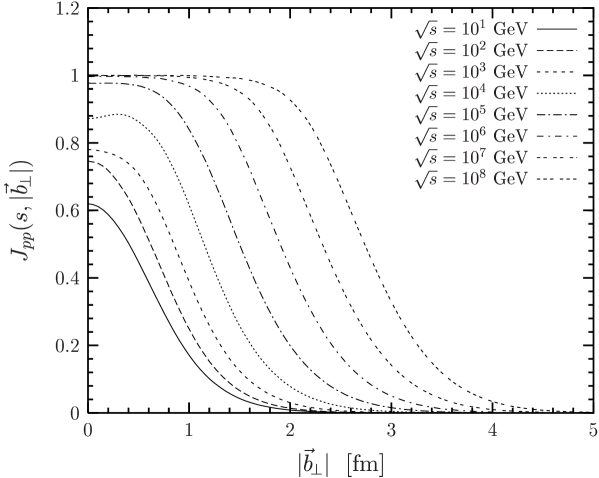
Figure 6.1: The profile function for proton-proton scattering $J_{pp}(s,|\vec{b}_{\!\perp}|)$ as a function of the impact parameter $|\vec{b}_{\!\perp}|$ for c.m. energies from $\sqrt{s}=10\,\mbox{GeV}$ to $10^{8}\,\mbox{GeV}$. The unitarity limit (6.4) corresponds to $J_{pp}(s,|\vec{b}_{\!\perp}|)=2$ and the black disc limit (6.6) to $J_{pp}(s,|\vec{b}_{\!\perp}|)=1$.

Up to $\sqrt{s}\approx 100\,\mbox{GeV}$, the profile has approximately a Gaussian shape. Above $\sqrt{s}=1\,\mbox{TeV}$, it develops into a broader and higher profile until the black disc limit is reached for $\sqrt{s}\approx 10^{6}\,\mbox{GeV}$ and $|\vec{b}_{\!\perp}|=0$. At this point, the cosine functions in $S_{DD}$ average to zero

$$\int\!\!dz_{1}d^{2}r_{1}\!\int\!\!dz_{2}d^{2}r_{2}|\psi_{p}(z_{1},{\vec{r}}_{1})|^{2}|\psi_{p}(z_{2},{\vec{r}}_{2})|^{2}S_{DD}(\sqrt{s}\gtrsim 10^{6}\,\mbox{GeV},|\vec{b}_{\!\perp}|=0,\dots)\approx 0$$ (6.10)

so that the proton wave function normalization determines the maximum opacity

$$J_{pp}^{\mathrm{max}}=\int\!\!dz_{1}d^{2}r_{1}\!\int\!\!dz_{2}d^{2}r_{2}\,|\psi_{p}(z_{1},{\vec{r}}_{1})|^{2}\,|\psi_{p}(z_{2},{\vec{r}}_{2})|^{2}=1\ .$$ (6.11)

Once the maximum opacity is reached at a certain impact parameter, the height of the profile function saturates at that $|\vec{b}_{\!\perp}|$ while the width of the profile function extends towards larger impact parameters with increasing energy. Thus, multiple gluonic interactions important to respect the $S$-matrix unitarity constraint (6.3) lead to saturation for $\sqrt{s}\gtrsim 10^{6}\,\mbox{GeV}$.

The above behavior of the profile function illustrates the evolution of the proton with increasing c.m. energy. The proton is gray and of small transverse size at small $\sqrt{s}$ but becomes blacker and more transversally extended with increasing $\sqrt{s}$ until it reaches the black disc limit in its center at $\sqrt{s}\approx 10^{6}\,\mbox{GeV}$. Beyond this energy, the proton cannot become blacker in its central region but in its periphery with continuing transverse growth. Furthermore, the proton boundary stays diffusive as claimed also in [120].

According to our model the black disc limit will not be reached at LHC. Our prediction of $\sqrt{s}\approx 10^{6}\,\mbox{GeV}=10^{3}\,\mbox{TeV}$ for the onset of the black disc limit in proton-proton collisions is about two orders of magnitude beyond the LHC energy $\sqrt{s}=14\,\mbox{TeV}$. This is in contrast to, e.g. [121], where the value predicted for the onset of the black disc limit is $\sqrt{s}=2\,\mbox{TeV}$, i.e. small enough to be reached at LHC. However, note that our profile function $J_{pp}(s,|\vec{b}_{\!\perp}|)$ yields good agreement with experimental data for cross sections up to the highest energies as shown in Chap. 7.

For hadron-hadron reactions in general, the wave function normalization of the hadrons determines the maximum opacity analogous to (6.11) and the transverse hadron size the c.m. energy at which it is reached. Consequently, the maximum opacity obtained for $\pi p$ and $Kp$ scattering is identical to the one for $pp$ scattering due to the normalization (5.2). The smaller size of pions and kaons in comparison to protons, however, demands slightly higher c.m. energies to reach this maximum opacity. Such size effects become more pronounced in longitudinal photon-proton scattering, where the size of the dipole emerging from the photon can be controlled by the photon virtuality.

6.3 The Profile Function for Photon-Proton Scattering

The profile function for a longitudinal photon $\gamma_{L}^{*}$ scattering off a proton $p$

$$J_{\gamma_{L}^{*}p}(s,|\vec{b}_{\!\perp}|,Q^{2}) = \int\!\!dz_{1}d^{2}r_{1}\!\int\!\!dz_{2}d^{2}r_{2}\,|\psi_{\gamma_{L}^{*}}(z_{1},\vec{r}_{1},Q^{2})|^{2}\,|\psi_{p}(z_{2},\vec{r}_{2})|^{2}$$ (6.12)

$$\times\left[1-S_{DD}(\vec{b}_{\!\perp},s,z_{1},{\vec{r}}_{1},z_{2},{\vec{r}}_{2})\right]$$

is calculated with the longitudinal photon wave function $|\psi_{\gamma_{L}^{*}}(z_{i},\vec{r}_{i},Q^{2})|^{2}$ given in (5.5). In this way, the profile function (6.12) is ideally suited for the investigation of dipole size effects since the photon virtuality $Q^{2}$ determines the transverse size of the dipole into which the photon fluctuates before it interacts with the proton.

Figure 6.2 shows the $|\vec{b}_{\!\perp}|$ dependence of the profile function $J_{\gamma_{L}^{*}p}(s,|\vec{b}_{\!\perp}|,Q^{2})$ divided by $\alpha/{\pi}$ at a photon virtuality of $Q^{2}=1\,\mbox{GeV}^{2}$ for c.m. energies $\sqrt{s}$ from $10\,\mbox{GeV}$ to $10^{9}\,\mbox{GeV}$, where $\alpha$ is the fine-structure constant.

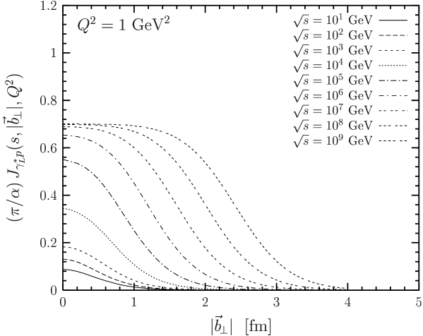
Figure 6.2: The profile function for a longitudinal photon scattering off a proton $J_{\gamma_{L}^{*}p}(s,|\vec{b}_{\!\perp}|,Q^{2})$ divided by $\alpha/{\pi}$ as a function of the impact parameter $|\vec{b}_{\!\perp}|$ at a photon virtuality of $Q^{2}=1\,\mbox{GeV}^{2}$ and c.m. energies from $\sqrt{s}=10\,\mbox{GeV}$ to $10^{9}\,\mbox{GeV}$. The value of the black disc limit is $J_{\gamma_{L}^{*}p}^{\mathrm{max}}(Q^{2}=1\,\mbox{GeV}^{2})=0.00164$ .

One clearly sees that the qualitative behavior of this rescaled profile function is similar to the one for proton-proton scattering. However, the black disc limit induced by the underlying dipole-dipole scattering depends on the photon virtuality $Q^{2}$ and is given by the normalization of the longitudinal photon wave function

$$J_{\gamma_{L}^{*}p}^{\mathrm{max}}(Q^{2})=\int\!\!dzd^{2}r|\psi_{\gamma_{L}^{*}}(z,\vec{r},Q^{2})|^{2}$$ (6.13)

since the proton wave function is normalized to one.

The photon virtuality $Q^{2}$ does not only determine the absolute value of the black disc limit but also the c.m. energy at which it is reached. This is illustrated in Fig. 6.3, where the $\sqrt{s}$ dependence of $J_{\gamma_{L}^{*}p}(s,|\vec{b}_{\!\perp}|=0,Q^{2})$ divided by $\alpha/{\pi}$ is presented for $Q^{2}=1,\,10,\,\mbox{and}\,100\,\mbox{GeV}^{2}$.

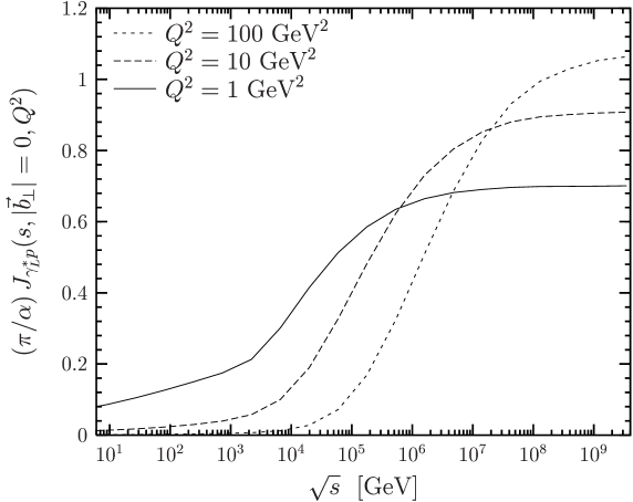
Figure 6.3: The profile function for a longitudinal photon scattering off a proton $J_{\gamma_{L}^{*}p}(s,|\vec{b}_{\!\perp}|,Q^{2})$ divided by $\alpha/{\pi}$ as a function of the c.m. energy $\sqrt{s}$ at zero impact parameter ($|\vec{b}_{\!\perp}|=0$) for photon virtualities of $Q^{2}=1,\,10,\,\mbox{and}\,100\,\mbox{GeV}^{2}$.

With increasing resolution $Q^{2}$, i.e. decreasing dipole sizes, $|\vec{r}_{\gamma_{L}^{*}}|^{2}\propto 1/Q^{2}$, the absolute value of the black disc limit grows and higher energies are needed to reach this limit. The growth of the absolute value of the black disc limit is simply due to the normalization of the longitudinal photon wave function while the need for higher energies to reach this limit is due to the decreasing interaction strength with decreasing dipole size. The latter explains also why the energies needed to reach the black disc limit in $\pi p$ and $Kp$ scattering are higher than in $pp$ scattering. Comparing $\gamma_{L}^{*}p$ scattering at $Q^{2}=1\,\mbox{GeV}^{2}$ with $pp$ scattering quantitatively, the black disc limit $J_{\gamma_{L}^{*}p}^{\mathrm{max}}(Q^{2}=1\,\mbox{GeV}^{2})=0.00164$ is about three orders of magnitude smaller because of the photon wave function normalization ($\propto\alpha/{\pi}$). At $|\vec{b}_{\!\perp}|=0$ it is reached at an energy of $\sqrt{s}\approx 10^{8}\,\mbox{GeV}$, which is about two orders of magnitude higher because of the smaller dipoles involved.

The way in which the profile function $J_{\gamma_{L}^{*}p}(s,|\vec{b}_{\!\perp}|,Q^{2})$ approaches the black disc limit at high energies depends on the shape of the proton and longitudinal photon wave function at small dipole sizes $|\vec{r}_{1,2}|$. At high energies, dipoles of typical sizes $0\leq|\vec{r}_{1,2}|\leq R_{0}\,(s_{0}/s)^{1/4}$ give the main contribution to $S_{\gamma_{L}^{*}p}=1-J_{\gamma_{L}^{*}p}$ because of (5.13) and the fact that the contribution of the large dipole sizes averages to zero upon integration over the dipole orientations, cf. also (6.10). Since $S_{\gamma_{L}^{*}p}$ is a measure of the proton transmittance, this means that only small dipoles can penetrate the proton at high energies. Increasing the energy further, even these small dipoles are absorbed and the black disc limit is reached. However, the dependence of the profile function on the short distance behavior of normalizable wave functions is weak which can be understood as follows. Because of color transparency, the eikonal functions $\chi^{N\!P}(s)$ and $\chi^{P}(s)$ are small for small dipole sizes $0\leq|\vec{r}_{1,2}|\leq R_{0}\,(s_{0}/s)^{1/4}$ at large $\sqrt{s}$. Consequently, $S_{DD}\approx 1$ and

$$\!\!\!\!\!\!\!\!\!\!\!\!\!\!\!\!J_{\gamma_{L}^{*}p}(s,|\vec{b}_{\!\perp}|,Q^{2})$$

$$\!\!\!\!\!\!\!\!\!\!\!\!\!\!\!\!\approx J_{\gamma_{L}^{*}p}^{\mathrm{max}}(Q^{2})-4\pi^{2}\!\!\int\limits_{0}^{1}\!\!dz_{1}\!\!\int\limits_{0}^{r_{c}(s)}\!\!\!dr_{1}r_{1}|\psi_{\gamma_{L}^{*}}(z_{1},r_{1},Q^{2})|^{2}\int\limits_{0}^{1}\!\!dz_{2}\!\!\int\limits_{0}^{r_{c}(s)}\!\!\!dr_{2}r_{2}|\psi_{p}(z_{2},r_{2})|^{2}$$ (6.14)

where $r_{c}(s)\approx R_{0}\,(s_{0}/s)^{1/4}$. Clearly, the linear behavior from the phase space factors $r_{1,2}$ dominates over the $r_{1,2}$-dependence of normalizable wave functions. More generally, for any profile function involving normalizable wave functions, the way in which the black disc limit is approached depends only weakly on the short distance behavior of the wave functions.

6.4 A Scenario for Gluon Saturation

In this section we discuss saturation of the impact parameter dependent gluon distribution of the proton $xG(x,Q^{2},|\vec{b}_{\!\perp}|)$. Using a leading twist, next-to-leading order QCD relation between $xG(x,Q^{2})$ and the longitudinal structure function $F_{L}(x,Q^{2})$, we relate $xG(x,Q^{2},|\vec{b}_{\!\perp}|)$ to the profile function $J_{\gamma_{L}^{*}p}(s=Q^{2}/x,|\vec{b}_{\!\perp}|,Q^{2})$ and find low-$x$ saturation of $xG(x,Q^{2},|\vec{b}_{\!\perp}|)$ as a manifestation of $S$-matrix unitarity. The resulting $xG(x,Q^{2},|\vec{b}_{\!\perp}|)$ is, of course, only an estimate since our profile function contains also higher twist contributions. Furthermore, in the considered low-$x$ region, the leading twist, next-to-leading order QCD formula may be inadequate as higher twist contributions [122] and higher order QCD corrections [123, 124] are expected to become important. Nevertheless, still assuming a close relation between $F_{L}(x,Q^{2})$ and $xG(x,Q^{2})$ at low $x$, we think that our approach provides some insight into the gluon distribution as a function of the impact parameter and into its saturation.

The gluon distribution of the proton $~{}xG(x,Q^{2})~{}$ is defined as follows: $xG(x,Q^{2})dx$ gives the momentum fraction of the proton which is carried by the gluons in the interval $[x,x+dx]$ as seen by probes of virtuality $Q^{2}$. The impact parameter dependent gluon distribution $xG(x,Q^{2},|\vec{b}_{\!\perp}|)$ is the gluon distribution $xG(x,Q^{2})$ at a given impact parameter $|\vec{b}_{\!\perp}|$ so that

$$xG(x,Q^{2})=\int\!\!d^{2}b_{\!\perp}\,xG(x,Q^{2},|\vec{b}_{\!\perp}|)\ .$$ (6.15)

In leading twist, next-to-leading order QCD, the gluon distribution $xG(x,Q^{2})$ is related to the structure functions $F_{L}(x,Q^{2})$ and $F_{2}(x,Q^{2})$ of the proton [125]

$$F_{L}(x,Q^{2})=\frac{\alpha_{s}}{\pi}\!\left[\frac{4}{3}\int_{x}^{1}\!\frac{dy}{y}\!\left(\frac{x}{y}\right)^{\!\!2}\!F_{2}(y,Q^{2})+2\sum_{f}e_{f}^{2}\!\int_{x}^{1}\!\frac{dy}{y}\!\left(\frac{x}{y}\right)^{\!\!2}\!\!\left(\!1-\frac{x}{y}\right)yG(y,Q^{2})\right]$$ (6.16)

where $\sum_{f}e_{f}^{2}$ is a flavor sum over the quark charges squared. For four active flavors and $x\lesssim 10^{-3}$, (6.16) can be approximated as follows [126]

$$xG(x,Q^{2})\approx\frac{3}{5}\,5.8\,\left[\frac{3\pi}{4\alpha_{s}}\,F_{L}(0.417x,Q^{2})-\frac{1}{1.97}\,F_{2}(0.75x,Q^{2})\right]\ .$$ (6.17)

For typical $\Lambda_{QCD}=100-300\,\mbox{MeV}$ and $Q^{2}=50-100\,\mbox{GeV}^{2}$, the coefficient of $F_{L}$ in (6.17), $3\pi/(4\alpha_{s})={\cal{O}}(10)$, is large compared to the one of $F_{2}$. Taking into account also the values of $F_{2}$ and $F_{L}$, the gluon distribution is mainly determined by the longitudinal structure function for $x\lesssim 10^{-3}$ in this $Q^{2}$ region. The longitudinal structure function can be expressed in terms of the profile function for longitudinal photon-proton scattering using the optical theorem (cf. (7.1))

$$F_{L}(x,Q^{2})=\frac{Q^{2}}{4\,\pi^{2}\,\alpha}\,\sigma^{tot}_{\gamma^{*}_{L}p}(x,Q^{2})=\frac{Q^{2}}{4\,\pi^{2}\,\alpha}\,2\!\int\!\!d^{2}b_{\!\perp}\,J_{\gamma_{L}^{*}p}(x,|\vec{b}_{\!\perp}|,Q^{2})\ ,$$ (6.18)

where the $s$-dependence of the profile function is rewritten in terms of the Bjorken scaling variable $x=Q^{2}/s$. Thus, neglecting the $F_{2}$ term in (6.17), the gluon distribution reduces to

$$xG(x,Q^{2})\approx 1.305\,\frac{Q^{2}}{\pi^{2}\alpha_{s}}\,\frac{\pi}{\alpha}\int\!\!d^{2}b_{\!\perp}\,J_{\gamma_{L}^{*}p}(0.417x,|\vec{b}_{\!\perp}|,Q^{2})\ .$$ (6.19)

Comparing (6.15) with (6.19), it seems natural to relate the integrand of (6.19) to the impact parameter dependent gluon distribution

$$xG(x,Q^{2},|\vec{b}_{\!\perp}|)\approx 1.305\,\frac{Q^{2}}{\pi^{2}\alpha_{s}}\,\frac{\pi}{\alpha}\,J_{\gamma_{L}^{*}p}(0.417x,|\vec{b}_{\!\perp}|,Q^{2})\ .$$ (6.20)

The black disc limit of the profile function for longitudinal photon-proton scattering (6.13) imposes accordingly an upper bound on $xG(x,Q^{2},|\vec{b}_{\!\perp}|)$

$$xG(x,Q^{2},|\vec{b}_{\!\perp}|)\ \leq\ xG^{\mathrm{max}}(Q^{2})\approx 1.305\,\frac{Q^{2}}{\pi^{2}\alpha_{s}}\,\frac{\pi}{\alpha}\,J_{\gamma^{*}_{L}p}^{\mathrm{max}}(Q^{2})\ ,$$ (6.21)

which is the low-$x$ saturation value of the gluon distribution $xG(x,Q^{2},|\vec{b}_{\!\perp}|)$ in our approach. With $\pi J_{\gamma^{*}_{L}p}^{\mathrm{max}}(Q^{2})/\alpha\approx 1$ as shown in Fig. 6.3, a compact approximation of (6.21) is obtained

$$xG(x,Q^{2},|\vec{b}_{\!\perp}|)\ \leq\ xG^{\mathrm{max}}(Q^{2})\approx\frac{Q^{2}}{\pi^{2}\alpha_{s}}\ ,$$ (6.22)

which is consistent with the results in [124, 127, 128] and indicates strong color field strengths $G^{a}_{\mu\nu}\sim 1/\sqrt{\alpha_{s}}$ as well.

According to our relations (6.20) and (6.21), the blackness described by the profile function is a measure for the gluon distribution and the black disc limit corresponds to the maximum gluon distribution reached at the impact parameter under consideration. In accordance with the behavior of the profile function $J_{\gamma_{L}^{*}p}$, see Fig. 6.2, the gluon distribution $xG(x,Q^{2},|\vec{b}_{\!\perp}|)$ decreases with increasing impact parameter for given values of $x$ and $Q^{2}$. Consequently, the gluon density has its maximum in the geometrical center of the proton, i.e. at zero impact parameter, and decreases towards the periphery. With decreasing $x$ at given $Q^{2}$, the gluon distribution $xG(x,Q^{2},|\vec{b}_{\!\perp}|)$ increases and extends towards larger impact parameters just as the profile function $J_{\gamma_{L}^{*}p}$ for increasing $s$. The saturation of the gluon distribution $xG(x,Q^{2},|\vec{b}_{\!\perp}|)$ sets in first in the center of the proton ($|\vec{b}_{\!\perp}|=0$) at very small Bjorken $x$.

In Fig. 6.4 the gluon distribution $xG(x,Q^{2},|\vec{b}_{\!\perp}|=0)$ is shown as a function of $x$ for $Q^{2}=1,\,10,\,\mbox{and}\,100\,\mbox{GeV}^{2}$, where relation (6.20) has been used also for low photon virtualities.

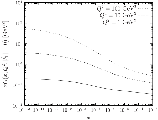
Figure 6.4: The gluon distribution of the proton at zero impact parameter $xG(x,Q^{2},|\vec{b}_{\!\perp}|=0)$ as a function of $x$ for $Q^{2}=1,\,10,\,\mbox{and}\,100\,\mbox{GeV}^{2}$. The results are obtained within approximation (6.20).

Evidently, the gluon distribution $xG(x,Q^{2},|\vec{b}_{\!\perp}|=0)$ saturates at very low values of $x\lesssim 10^{-10}$ for $Q^{2}\gtrsim 1\,\mbox{GeV}^{2}$. The photon virtuality $Q^{2}$ determines the saturation value (6.21) and the Bjorken $x$ at which it is reached; cf. also Fig. 6.2. For larger $Q^{2}$, the low-$x$ saturation value is larger and is reached at smaller values of $x$, as claimed also in [129]. Moreover, the growth of $xG(x,Q^{2},|\vec{b}_{\!\perp}|=0)$ with decreasing $x$ becomes stronger with increasing $Q^{2}$. This results from the stronger energy increase of the perturbative component, $\epsilon^{P}=0.73$, that becomes more important with decreasing dipole size.

According to our approach, the onset of the $xG(x,Q^{2},|\vec{b}_{\!\perp}|)$-saturation appears for $Q^{2}\gtrsim 1\,\mbox{GeV}^{2}$ at $x\lesssim 10^{-10}$, which is far below the $x$-region accessible at HERA ($x\gtrsim 10^{-6}$). Even for THERA ($x\gtrsim 10^{-7}$), gluon saturation is not predicted for $Q^{2}\gtrsim 1\,\mbox{GeV}^{2}$. However, since the HERA data can be described by models with and without saturation embedded [129], the present situation is not conclusive.

Note that the $S$-matrix unitarity condition (6.3) together with (6.20) requires the saturation of the impact parameter dependent gluon distribution $xG(x,Q^{2},|\vec{b}_{\!\perp}|)$ but not the saturation of the integrated gluon distribution $xG(x,Q^{2})$. Due to multiple gluonic interactions in our model, this requirement is fulfilled, as can be seen from Fig. 6.2 and relation (6.20). Indeed, approximating the gluon distribution $xG(x,Q^{2},|\vec{b}_{\!\perp}|)$ in the saturation regime of very low $x$ by a step-function

$$xG(x,Q^{2},|\vec{b}_{\!\perp}|)\approx xG^{\mathrm{max}}(Q^{2})\,\Theta(\,R(x,Q^{2})-|\vec{b}_{\!\perp}|\,)\ ,$$ (6.23)

where $R(x,Q^{2})$ denotes the full width at half maximum of the profile function, one obtains with (6.15), (6.21) and (6.22) the integrated gluon distribution

$$xG(x,Q^{2})\;\approx\;1.305\,\frac{Q^{2}\,R^{2}(x,Q^{2})}{\pi\alpha_{s}}\,\frac{\pi}{\alpha}\,J_{\gamma^{*}_{L}p}^{\mathrm{max}}(Q^{2})\;\approx\;\frac{Q^{2}\,R^{2}(x,Q^{2})}{\pi\alpha_{s}}\ ,$$ (6.24)

which does not saturate because of the increase of the effective proton radius $R(x,Q^{2})$ with decreasing $x$. Nevertheless, although $xG(x,Q^{2})$ does not saturate, the saturation of $xG(x,Q^{2},|\vec{b}_{\!\perp}|)$ leads to a slow-down in its growth towards small $x$. Interestingly, our result (6.24) coincides with the result of Mueller and Qiu [124].

Finally, it must be emphasized that the low-$x$ saturation of $xG(x,Q^{2},|\vec{b}_{\!\perp}|)$, required in our approach by the $S$-matrix unitarity, is realized by multiple gluonic interactions. In other approaches that describe the evolution of the gluon distribution with varying $x$ and $Q^{2}$, gluon recombination leads to gluon saturation [123, 124, 131, 132, 133], which is reached when the probability of a gluon splitting up into two is equal to the probability of two gluons fusing into one. A more phenomenological understanding of saturation is attempted in [113, 134].

Chapter 7 Comparison with Experimental Data

In this chapter we present the phenomenological performance of our model. We compute total, differential, and elastic cross sections, structure functions, and diffractive slopes for hadron-hadron, photon-proton, and photon-photon scattering, compare the results with experimental data including cosmic ray data, and provide predictions for future experiments. Having studied the saturation of the impact parameter profiles, we show here how this manifestation of unitarity translates into the quantities mentioned above and how it could become observable.

Using the $T$-matrix (5.15) with the wave functions and parameters from Secs. 5.1 and 5.3, we compute the pomeron contribution to $pp$, $p{\bar{p}}$, $\pi^{\pm}p$, $K^{\pm}p$, $\gamma^{*}p$, and $\gamma\gamma$ reactions in terms of the universal dipole-dipole scattering amplitude $S_{DD}$. This allows one to compare reactions induced by hadrons and photons in a systematic way. In fact, it is our aim to provide a unified description of all these reactions and to show in this way that the pomeron contribution to the above reactions is universal and can be traced back to the dipole-dipole scattering amplitude $S_{DD}$.

Our model describes pomeron ($C=+1$ gluon exchange) but neither odderon ($C=-1$ gluon exchange) nor reggeon exchange (quark-antiquark exchange) as discussed in Sec. 4.3. Only in the computation of the hadronic total cross sections the reggeon contribution is added [115, 59]. This improves the agreement with the data for $\sqrt{s}\lesssim 100\,\mbox{GeV}$ and describes exactly the differences between $ab$ and $\bar{a}b$ reactions.

The fine tuning of the model and wave function parameters was performed on the data shown below. The resulting parameter set given in Secs. 5.1 and 5.3 is used throughout this chapter.

7.1 Total Cross Sections

The total cross section for the high-energy reaction $ab\to X$ is related via the optical theorem to the imaginary part of the forward elastic scattering amplitude and can also be expressed in terms of the profile function (6.2)

$$\sigma^{tot}_{ab}(s)\;=\;\frac{1}{s}\,\mbox{Im}\,T(s,t=0)\;=\;2\int\!d^{2}b_{\!\perp}\,J_{ab}(s,|\vec{b}_{\!\perp}|)\ ,$$ (7.1)

where $a$ and $b$ label the initial particles whose masses were neglected as they are small in comparison to the c.m. energy $\sqrt{s}$.

We compute the pomeron contribution to the total cross section, $\sigma^{tot,I\!\!P}_{ab}(s)$, from the $T$-matrix (5.15), as explained above, and add only here a reggeon contribution of the form [115, 59]

$$\sigma^{tot,I\!\!R}_{ab}(s)=X_{ab}\,\left(\frac{s}{1\,\mbox{GeV}^{2}}\right)^{-0.4525}\ ,$$ (7.2)

where $X_{ab}$ depends on the reaction considered: $X_{pp}=56.08\,\mbox{mb}$, $X_{p{\bar{p}}}=98.39\,\mbox{mb}$, $X_{\pi^{+}p}=27.56\,\mbox{mb}$, $X_{\pi^{-}p}=36.02\,\mbox{mb}$, $X_{K^{+}p}=8.15\,\mbox{mb}$, $X_{K^{-}p}=26.36\,\mbox{mb}$, $X_{\gamma p}=0.129\,\mbox{mb}$, and $X_{\gamma\gamma}=605\,\mbox{nb}$. Accordingly, we obtain the total cross section

$$\sigma^{tot}_{ab}(s)=\sigma^{tot,I\!\!P}_{ab}(s)+\sigma^{tot,I\!\!R}_{ab}(s)$$ (7.3)

for $pp$, $p{\bar{p}}$, $\pi^{\pm}p$, $K^{\pm}p$, $\gamma p$, and $\gamma\gamma$ scattering.

The good agreement of the computed total cross sections with the experimental data is shown in Fig. 7.1.

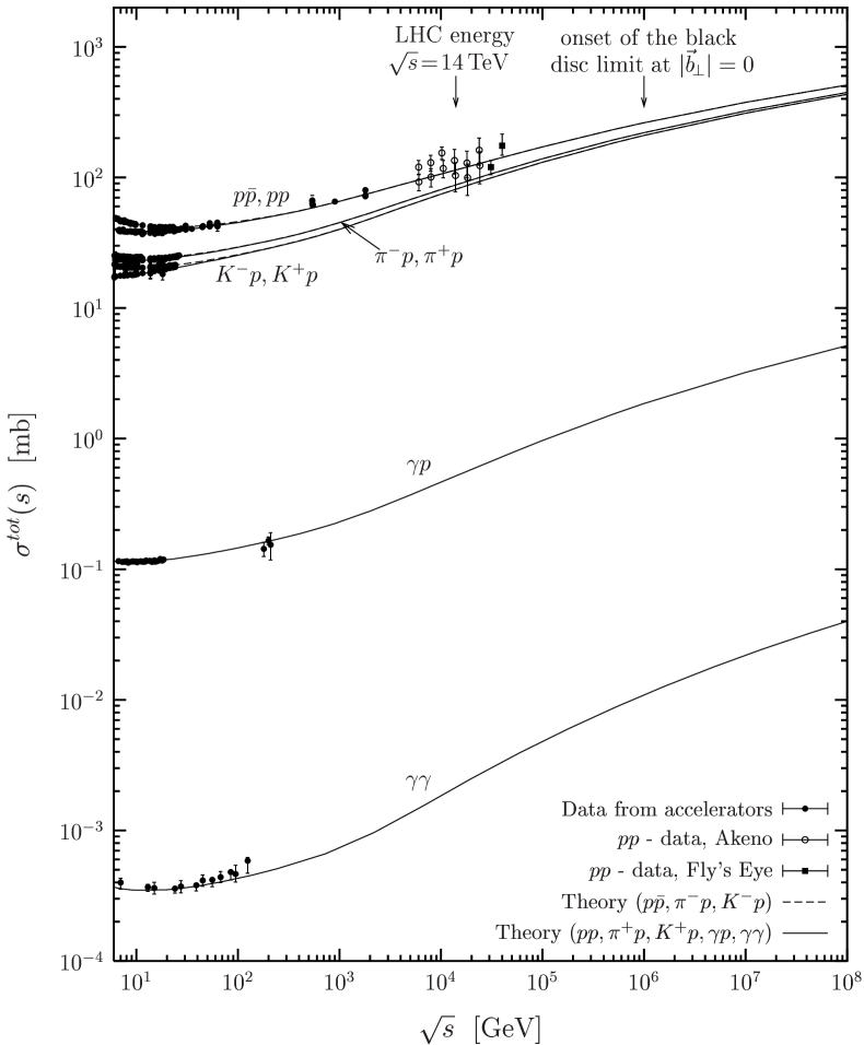
Figure 7.1: The total cross section $\sigma^{tot}$ as a function of the c.m. energy $\sqrt{s}$ for $pp$, $p{\bar{p}}$, $\pi^{\pm}p$, $K^{\pm}p$, $\gamma p$, and $\gamma\gamma$ scattering. The solid lines represent the model results for $pp$, $\pi^{+}p$, $K^{+}p$, $\gamma p$ and $\gamma\gamma$ scattering and the dashed lines the ones for $p{\bar{p}}$, $\pi^{-}p$, and $K^{-}p$ scattering. The $pp$, $p{\bar{p}}$, $\pi^{\pm}p$, $K^{\pm}p$, $\gamma p$ [10] and $\gamma\gamma$ data [135] taken at accelerators are indicated by the closed circles while the closed squares (Fly’s eye data) [136] and the open circles (Akeno data) [137] indicate cosmic ray data. The arrows at the top point to the LHC energy, $\sqrt{s}=14\,\mbox{TeV}$, and to the onset of the black disc limit in $pp$ ($p{\bar{p}}$) reactions, $\sqrt{s}\approx 10^{6}\,\mbox{GeV}$.

Here the solid lines represent the theoretical results for $pp$, $\pi^{+}p$, $K^{+}p$, $\gamma p$, and $\gamma\gamma$ scattering and the dashed lines the ones for $p{\bar{p}}$, $\pi^{-}p$, and $K^{-}p$ scattering. The $pp$, $p{\bar{p}}$, $\pi^{\pm}p$, $K^{\pm}p$, $\gamma p$ [10] and $\gamma\gamma$ data [135] taken at accelerators are indicated by the closed circles while the closed squares (Fly’s eye data) [136] and the open circles (Akeno data) [137] indicate cosmic ray data. Only real photons are considered which are, of course, transverse polarized.

The prediction for the total $pp$ cross section at LHC ($\sqrt{s}=14\,\mbox{TeV}$) is $\sigma^{tot}_{pp}=114.2\,\mbox{mb}$ in good agreement with cosmic ray data. Compared with other works, our LHC prediction is close to the one of Block et al. [138], $\sigma^{tot}_{pp}=108\pm 3.4\,\mbox{mb}$, but considerably larger than the one of Donnachie and Landshoff [115], $\sigma^{tot}_{pp}=101.5\,\mbox{mb}$.

The differences between $ab$ and $\bar{a}b$ reactions for $\sqrt{s}\lesssim 100\,\mbox{GeV}$ result solely from the different reggeon contributions which die out rapidly as the energy increases. The pomeron contribution to $ab$ and $\bar{a}b$ reactions is, in contrast, identical and increases as the energy increases. It thus governs the total cross sections for $\sqrt{s}\gtrsim 100\,\mbox{GeV}$ where the results for $ab$ and $\bar{a}b$ reactions coincide.

The differences between $pp$ ($p{\bar{p}}$), $\pi^{\pm}p$, and $K^{\pm}p$ scattering result from the different transverse extension parameters, $S_{p}=0.86\,\mbox{fm}>S_{\pi}=0.607\,\mbox{fm}>S_{K}=0.55\,\mbox{fm}$, cf. Sec. 5.1. Since a smaller transverse extension parameter favors smaller dipoles, the total cross section becomes smaller and the short distance physics described by the perturbative component becomes more important which leads to a stronger energy growth due to $\epsilon^{P}=0.73>\epsilon^{N\!P}=0.125$. In fact, the ratios $\sigma^{tot}_{pp}/\sigma^{tot}_{\pi p}$ and $\sigma^{tot}_{pp}/\sigma^{tot}_{Kp}$ converge slowly towards unity with increasing energy as can already be seen in Fig. 7.1.

For real photons, the transverse size is governed by the constituent quark masses $m_{f}(Q^{2}=0)$, cf. Sec. 5.1, where the light quarks have the strongest effect, i.e. $\sigma^{tot}_{\gamma p}\propto 1/m_{u,d}^{2}$ and $\sigma^{tot}_{\gamma\gamma}\propto 1/m_{u,d}^{4}$. Furthermore, in comparison with hadron-hadron scattering, there is the additional suppression factor of $\alpha$ for $\gamma p$ and $\alpha^{2}$ for $\gamma\gamma$ scattering coming from the photon-dipole transition. In the $\gamma\gamma$ reaction, also the box diagram contributes [139, 59] but is neglected since its contribution to the total cross section is less than 1% [60].

It is worthwhile mentioning that total cross sections for $pp$ ($p{\bar{p}}$), $\pi^{\pm}p$, and $K^{\pm}p$ scattering do not depend on the longitudinal quark momentum distribution in the hadrons since the underlying dipole-dipole cross section is independent of the longitudinal quark momentum fraction $z_{i}$ for $t=0$. We have shown this analytically on the two-gluon-exchange level in [24].

Saturation effects as a manifestation of the $S$-matrix unitarity can be seen in Fig. 7.1. Having investigated the profile function for $pp$ ($p{\bar{p}}$) scattering, we know that this profile function becomes higher and broader with increasing energy until it saturates the black disc limit first for zero impact parameter ($|\vec{b}_{\!\perp}|=0$) at $\sqrt{s}\approx 10^{6}\,\mbox{GeV}$. Beyond this energy, the profile function cannot become higher but expands towards larger values of $|\vec{b}_{\!\perp}|$. Consequently, the total cross section (7.1) increases no longer due to the growing blackness at the center but only due to the transverse expansion of the hadrons. This tames the growth of the total cross section as can be seen for the total $pp$ cross section beyond $\sqrt{s}\approx 10^{6}\,\mbox{GeV}$ in Fig. 7.1.

At energies beyond the onset of the black disc limit at zero impact parameter, the profile function can be approximated by

$$J_{ab}^{\mathrm{approx}}(s,|\vec{b}_{\!\perp}|)=N_{a}\,N_{b}\,\Theta\left(R(s)-|\vec{b}_{\!\perp}|\right)\,$$ (7.4)

where $N_{a,b}$ denotes the normalization of the wave functions of the scattered particles and $R(s)$ the full width at half maximum of the exact profile function $J_{ab}(s,|\vec{b}_{\!\perp}|)$ that reflects the effective radii of the interacting particles. Thus, the energy dependence of the total cross section (7.1) is driven exclusively by the increase of the transverse extension of the particles $R(s)$

$$\sigma^{tot}_{ab}(s)=2\pi N_{a}N_{b}R(s)^{2}\ ,$$ (7.5)

which is known as geometrical scaling [140, 118]. The growth of $R(s)$ can at most be logarithmic for $\sqrt{s}\to\infty$ because of the Froissart bound [18]. In fact, a transition from a power-like to an $\ln^{2}$-increase of the total $pp$ cross section seems to set in at about $\sqrt{s}\approx 10^{6}\,\mbox{GeV}$ as visible in Fig. 7.1. Moreover, since the hadronic cross sections join for $\sqrt{s}\to\infty$, $R(s)$ becomes independent of the hadron-hadron reaction considered at asymptotic energies as long as $N_{a,b}=1$. Also for photons of different virtuality $Q_{1}^{2}$ and $Q_{2}^{2}$ one can check that the ratio of the total cross sections $\sigma^{tot}_{\gamma^{*}p}(Q_{1}^{2})/\sigma^{tot}_{\gamma^{*}p}(Q_{2}^{2})$ converges to unity at asymptotic energies in agreement with the conclusion in [141].

7.2 The Proton Structure Function

The total cross section for the scattering of a transverse ($T$) and longitudinally ($L$) polarized photon off the proton, $\sigma_{\gamma^{*}_{T\!,L}p}^{tot}(x,Q^{2})$, at photon virtuality $Q^{2}$ and c.m. energy squared $s=Q^{2}/x$ is equivalent to the structure functions of the proton

$$F_{T,L}(x,Q^{2})=\frac{Q^{2}}{4\pi^{2}\alpha}\sigma_{\gamma^{*}_{T\!,L}p}^{tot}(x,Q^{2})$$ (7.6)

and

$$F_{2}(x,Q^{2})=F_{T}(x,Q^{2})+F_{L}(x,Q^{2})\ .$$ (7.7)

Reactions induced by virtual photons are particularly interesting because the transverse separation of the quark-antiquark pair that emerges from the virtual photon decreases as the photon virtuality increases (cf. Sec. 5.1)

$$|\vec{r}_{\gamma}|\approx\frac{2}{\sqrt{Q^{2}+4m_{u,d}^{2}}}\ ,$$ (7.8)

where $m_{u,d}$ is a mass of the order of the constituent $u$-quark mass. With increasing virtuality, one probes therefore smaller transverse distance scales of the proton.

In Fig. 7.2 the $Q^{2}$-dependence of the total $\gamma^{*}p$ cross section

$$\sigma^{tot}_{\gamma^{*}p}(s,Q^{2})=\sigma^{tot}_{\gamma_{T}^{*}p}(s,Q^{2})+\sigma^{tot}_{\gamma_{L}^{*}p}(s,Q^{2})$$ (7.9)

is presented, where the model results (solid lines) are compared with the experimental data for c.m. energies from $\sqrt{s}=20\,\mbox{GeV}$ up to $245\,\mbox{GeV}$. Note the indicated scaling factors at different $\sqrt{s}$ values. The low-energy data at $\sqrt{s}=20\,\mbox{GeV}$ are from [142] while the data at higher energies have been measured at HERA by the H1 [143, 11] and ZEUS collaboration [144, 13]. At $Q^{2}=0.012\,\mbox{GeV}^{2}$, also the photoproduction ($Q^{2}=0$) data from [145] are displayed.

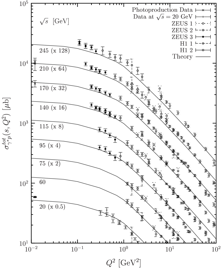
Figure 7.2: The total $\gamma^{*}p$ cross section $\sigma^{tot}_{\gamma^{*}p}(s,Q^{2})$ as a function of the photon virtuality $Q^{2}$ for c.m. energies from $\sqrt{s}=20\,\mbox{GeV}$ to $245\,\mbox{GeV}$, where the model results (solid lines) and the experimental data at different $\sqrt{s}$ values are scaled with the indicated factors. The low energy data at $\sqrt{s}=20\,\mbox{GeV}$ are from [142], the data at higher energies from the H1 [143, 11] and ZEUS collaboration [144, 13]. The photoproduction ($Q^{2}=0$) data from [145] are displayed at $Q^{2}=0.012\,\mbox{GeV}^{2}$.

The model results are in reasonable agreement with the experimental data in the window shown in Fig. 7.2. The total $\gamma^{*}p$ cross section levels off towards small values of $Q^{2}$ as soon as the photon size $|\vec{r}_{\gamma}|$, i.e the resolution scale, becomes comparable to the proton size. Our model reproduces this behavior by using the perturbative photon wave functions with $Q^{2}$-dependent quark masses, $m_{f}(Q^{2})$, that interpolate between the current (large $Q^{2}$) and the constituent (small $Q^{2}$) quark masses as explained in detail in Sec. 5.1. The decrease of $\sigma^{tot}_{\gamma^{*}p}$ with increasing $Q^{2}$ results from decreasing dipole sizes and the fact that small dipoles do not interact as strongly as large dipoles.

The $x$-dependence of the computed proton structure function $F_{2}(x,Q^{2})$ is shown in Fig. 7.3 for $Q^{2}=0.3,\,2.5,\,12,$ and $120\,\mbox{GeV}^{2}$ in comparison to the data measured by the H1 [146] and ZEUS [147] detector. Within our model, the increase of $F_{2}(x,Q^{2})$ towards small Bjorken $x$ becomes stronger with increasing $Q^{2}$ in agreement with the trend in the HERA data. This behavior results from the fast energy growth of the perturbative component that becomes more important with increasing $Q^{2}$ due to the smaller dipole sizes involved.

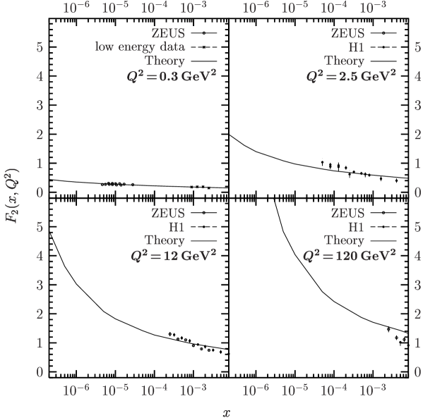
Figure 7.3: The $x$-dependence of the computed proton structure function $F_{2}(x,Q^{2})$ (solid line) for $Q^{2}=0.3,\,2.5,\,12,$ and $120\,\mbox{GeV}^{2}$ in comparison to the data measured by the H1 [146] and ZEUS [147] detector, and the low energy data at $\sqrt{s}=20\,\mbox{GeV}$ from [142].

As can be seen in Fig. 7.3, the data show a faster increase with decreasing $x$ than the model outside the low-$Q^{2}$ region. This results from the weak energy boost of the non-perturbative component that dominates $F_{2}(x,Q^{2})$ in our model. In fact, even for large $Q^{2}$ the non-perturbative contribution overwhelms the perturbative one, which explains also the overestimation of the data for $x\gtrsim 10^{-3}$.

This problem is typical for the SVM model applied to the scattering of a small size dipole off a proton. In an earlier application by Rüter [55], an additional cut-off was introduced to switch from the non-perturbative to the perturbative contribution as soon as one of the dipoles is smaller than $r_{cut}=0.16\,\mbox{fm}$. This yields a better agreement with the data also for large $Q^{2}$ but leads to a discontinuous dipole-proton cross section. In the model of Donnachie and Dosch [60], a similar SVM-based component is used also for dipoles smaller than $R_{c}=0.22\,\mbox{fm}$ with a strong energy boost instead of a perturbative component. Furthermore, their SVM-based component is tamed for large $Q^{2}$ by an additional $\alpha_{s}(Q^{2})$ factor.

We did not follow these lines in order to keep a continuous, $Q^{2}$-independent dipole-proton cross section and, therefore, cannot improve the agreement with the $F_{2}(x,Q^{2})$ data without losing quality in the description of hadronic observables. Since our non-perturbative component relies on lattice QCD, we are more confident in describing non-perturbative physics and thus put more emphasis on the hadronic observables. Admittedly, our model misses details of the proton structure that become visible with increasing $Q^{2}$. However, most other existing models provide neither the profile functions nor a simultaneous description of hadronic and $\gamma^{*}$-induced processes.

7.3 The Slope $B$ of Elastic Forward Scattering

The local slope of elastic scattering $B(s,t)$ is defined as

$$B(s,t):=\frac{d}{dt}\left(\ln\left[\frac{d\sigma^{el}}{dt}(s,t)\right]\right)$$ (7.10)

and characterizes the diffractive peak of the differential elastic cross section $d\sigma^{el}/dt(s,t)$ discussed below. Here we concentrate on the slope for elastic forward ($t=0$) scattering also called slope parameter

$$B(s):=B(s,t=0)=\frac{1}{2}\frac{\int\!d^{2}b_{\!\perp}\,|\vec{b}_{\!\perp}|^{2}\,J(s,|\vec{b}_{\!\perp}|)}{\int\!d^{2}b_{\!\perp}\,J(s,|\vec{b}_{\!\perp}|)}=\frac{1}{2}\langle b^{2}\rangle\ ,$$ (7.11)

which measures the root mean squared interaction radius $\langle b^{2}\rangle$ of the scattered particles, and does not depend on the opacity.

We compute the slope parameter with the profile function from the $T$-matrix (5.15) and neglect the reggeon contributions, which are relevant only at small c.m. energies, so that the same result is obtained for $ab$ and $\bar{a}b$ scattering.

In Fig. 7.4 the resulting slope parameter $B(s)$ is shown as a function of $\sqrt{s}$ for $pp$ and $p{\bar{p}}$ scattering (solid line) and compared with the $pp$ (open circles) and $p{\bar{p}}$ (closed circles) data from [148, 149, 150].

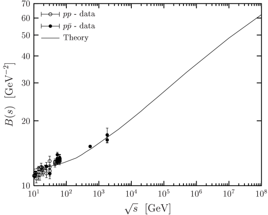
Figure 7.4: The elastic slope parameter $B(s)$ as a function of the c.m. energy $\sqrt{s}$ for $pp$ and $p{\bar{p}}$ forward ($t=0$) scattering. The solid line represents the model result that is compared to the data for $pp$ (open circles) and $p{\bar{p}}$ (closed circles) reactions from [148, 149, 150].

As expected from the opacity independence of the slope parameter (7.11), saturation effects as seen in the total cross sections do not occur. Indeed, one observes an approximate $B(s)\propto R^{2}(s)\propto\ln^{2}(\sqrt{s}/\sqrt{s_{0}})$ growth for $\sqrt{s}\gtrsim 10^{4}\,\mbox{GeV}$. This behavior agrees, of course, with the transverse expansion of $J_{pp}(s,|\vec{b}_{\!\perp}|)$ for increasing $\sqrt{s}$ shown in Fig. 6.1. Analogous results are obtained also for $\pi p$ and $Kp$ scattering.

For the good agreement of our model with the data, the finite width of the longitudinal quark momentum distribution in the hadrons, i.e. $\Delta z_{p},\,\Delta z_{\pi},\,\mbox{and}\,\Delta z_{K}\neq 0$ in (5.1), is important as the numerator in (7.11) depends on this width. In fact, $B(s)$ comes out more than 10% smaller with $\Delta z_{p},\,\Delta z_{\pi},\,\mbox{and}\,\Delta z_{K}=0$. Furthermore, a strong growth of the perturbative component, $\epsilon^{P}=0.73$, is important to achieve the increase of $B(s)$ for $\sqrt{s}\gtrsim 500\,\mbox{GeV}$ indicated by the data.

It must be emphasized that only the simultaneous fit of the total cross section and the slope parameter provides the correct shape of the profile function $J(s,|\vec{b}_{\!\perp}|)$. This shape leads then automatically to a good description of the differential elastic cross section $d\sigma^{el}/dt(s,t)$ as demonstrated below. Astonishingly, only few phenomenological models provide a satisfactory description of both quantities [138, 112]. In the approach of [57], for example, the total cross section is described correctly while the slope parameter exceeds the data by more than 20% already at $\sqrt{s}=23.5\,\mbox{GeV}$ and thus indicates deficiencies in the form of $J(s,|\vec{b}_{\!\perp}|)$.

7.4 The Differential Elastic Cross Section

The differential elastic cross section obtained from the squared absolute value of the $T$-matrix element

$$\frac{d\sigma^{el}}{dt}(s,t)=\frac{1}{16\pi s^{2}}|T(s,t)|^{2}$$ (7.12)

can be expressed for our purely imaginary $T$-matrix (5.15) in terms of the profile function

$$\frac{d\sigma^{el}}{dt}(s,t)=\frac{1}{4\pi}\left[\int\!\!d^{2}b_{\!\perp}\,e^{i{\vec{q}}_{\!\perp}{\vec{b}}_{\!\perp}}\,J(s,|\vec{b}_{\!\perp}|)\right]^{2}\ .$$ (7.13)

and is, thus, very sensitive to the transverse extension and opacity of the scattered particles. Equation (7.13) shows the analogy to optical diffraction, where $J(s,|\vec{b}_{\!\perp}|)$ describes the distribution of an absorber that causes the diffraction pattern observed for incident plane waves.

In Fig. 7.5 the differential elastic cross section computed for $pp$ and $p{\bar{p}}$ scattering (solid line) is shown as a function of $|t|=\vec{q}^{\,2}_{\!\perp}$ at $\sqrt{s}=23.5,\,30.7,\,44.7,\,63,\,546$, and $1800\,\mbox{GeV}$ and compared with experimental data (open circles), where the $pp$ data at $\sqrt{s}=23.5,\,30.7,\,44.7,\,\mbox{and}\,63\,\mbox{GeV}$ were measured at the CERN ISR [140], the $p{\bar{p}}$ data at $\sqrt{s}=546\,\mbox{GeV}$ at the CERN $Sp{{\bar{p}}}S$ [149], and the $p{\bar{p}}$ data at $\sqrt{s}=1.8\,\mbox{TeV}$ at the Fermilab Tevatron [150, 151]. The prediction of our model for the $pp$ differential elastic cross section at the CERN LHC, $\sqrt{s}=14\,\mbox{TeV}$, is given in Fig. 7.6.

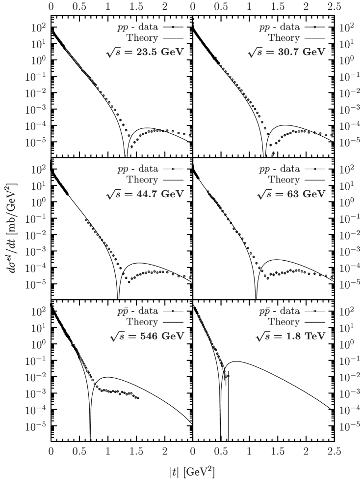
Figure 7.5: The differential elastic cross section for $pp$ and $p{\bar{p}}$ scattering as a function of $|t|$. The result of our model, indicated by the solid line, is compared for $\sqrt{s}=23.5,\,30.7,\,44.7,\,\mbox{and}\,63\,\mbox{GeV}$ with the CERN ISR $pp$ data [140], for $\sqrt{s}=546\,\mbox{GeV}$ with the CERN $Sp{{\bar{p}}}S$ data [149], and for $\sqrt{s}=1.8\,\mbox{TeV}$ with the Fermilab Tevatron $p{\bar{p}}$ data [150, 151], all indicated by the open circles with error bars.

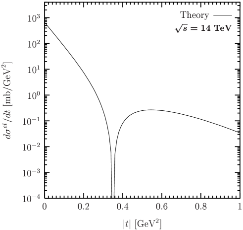
Figure 7.6: The prediction of our model for the $pp$ differential elastic cross section at LHC ($\sqrt{s}=14\,\mbox{TeV}$) as a function of momentum transfer $|t|$ up to $1\,\mbox{GeV}^{2}$.

For all energies, the model reproduces the experimentally observed diffraction pattern, i.e the characteristic diffraction peak at small $|t|$ and the dip structure at medium $|t|$. As the energy increases, also the shrinking of the diffraction peak is described which reflects the rise of the slope parameter $B(s,t=0)$ already discussed above. The shrinking of the diffraction peak comes along with a dip structure that moves towards smaller values of $|t|$ as the energy increases. This motion of the dip is also described approximately.

The dip in the theoretical curves reflects a change of sign in the $T$-matrix element (5.15). As the latter is purely imaginary, it is not surprising that there are deviations from the data in the dip region. Here the real part is expected to be important [151] which is in the small $|t|$ region negligible in comparison to the imaginary part.

The difference between the $pp$ and $p{\bar{p}}$ data, a deep dip for $pp$ but only a bump or shoulder for $p{\bar{p}}$ reactions, requires a $C=-1$ contribution. Besides the reggeon contribution at small energies, one expects here an additional perturbative $C=-1$ contribution such as three-gluon exchange [152, 153] or an odderon [154, 155, 156]. In fact, allowing a finite size diquark in the (anti-)proton an odderon appears that supports the dip in $pp$ but leads to the shoulder in $p{\bar{p}}$ reactions [156].

For the differential elastic cross section at the LHC energy, $\sqrt{s}=14\,\mbox{TeV}$, the above findings suggest an accurate prediction in the small-$|t|$ region but a dip at a position smaller than the predicted value at $|t|\approx 0.35\,\mbox{GeV}^{2}$. Our confidence in the validity of the model at small $|t|$ is supported additionally by the total cross section that fixes $d\sigma^{el}/dt(s,t=0)$ and is in agreement with the cosmic ray data shown in Fig. 7.1. Concerning our prediction for the dip position, it is close to the value $|t|\approx 0.41\,\mbox{GeV}^{2}$ of [138] but significantly below the value $|t|\approx 0.55\,\mbox{GeV}^{2}$ of [57]. Beyond the dip position, the height of the computed shoulder is always above the data and, thus, very likely to exceed also the LHC data. In comparison with other works, the height of our shoulder is similar to the one of [138] but almost one order of magnitude above the one of [57].

Considering Figs. 7.5 and 7.6 more quantitatively in the small-$|t|$ region, one can use the well known parametrization of the differential elastic cross section in terms of the slope parameter $B(s)$ and the curvature $C(s)$

$$d\sigma^{el}/dt(s,t)=d\sigma^{el}/dt(s,t=0)\,\exp\left[B(s)t+C(s)t^{2}\right]\ .$$ (7.14)

Using $B(s)$ from the preceding section and assuming for the moment $C(s)=0$, one achieves a good description at small momentum transfers and energies, which is consistent with the approximate Gaussian shape of $J_{pp}(s,|\vec{b}_{\!\perp}|)$ at small energies shown in Fig. 6.1. The dip, of course, is generated by the deviation from the Gaussian shape at small impact parameters. According to (7.14), the shrinking of the diffraction peak with increasing energy simply reflects the increasing interaction radius described by $B(s)$.

For small energies $\sqrt{s}$, our model reproduces the experimentally observed change in the slope at $|t|\approx 0.25\,\mbox{GeV}^{2}$ [157] that is characterized by a positive curvature. For LHC, we find clearly a negative value for the curvature in agreement with [138] but in contrast to [57]. The change of sign in the curvature reflects the transition of $J(s,|\vec{b}_{\!\perp}|)$ from the approximate Gaussian shape at low energies to the approximate step-function shape (7.4) at high energies.

Important for the good agreement with the data is the longitudinal quark momentum distribution in the proton. Besides the slope parameter, which characterizes the diffraction peak, also the dip position is very sensitive to the distribution width $\Delta z_{p}$, i.e. with $\Delta z_{p}=0$ the dip position appears at more than 10% lower values of $|t|$. In the earlier SVM approach [57], the reproduction of the correct dip position was possible without the $z$-dependence of the hadronic wave functions but a deviation from the data in the low-$|t|$ region had to be accepted. In this low-$|t|$ region, we achieved a definite improvement with the new correlation functions (2.50) and the minimal surfaces used in our model.

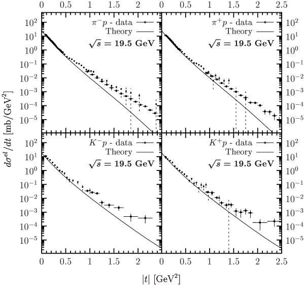
Figure 7.7: The differential elastic cross section $d\sigma^{el}/dt(s,t)$ as a function of $|t|$ for $\pi^{\pm}p$ and $K^{\pm}p$ reactions at a c.m. energy of $\sqrt{s}=19.5\,\mbox{GeV}$. The model results (solid line) are compared with the data (closed circles with error bars) from [158].

The differential elastic cross section computed for $\pi^{\pm}p$ and $K^{\pm}p$ reactions has the same behavior as the one for $pp$ ($p{\bar{p}}$) reactions. The only difference comes from the different $z$-distribution widths, $\Delta z_{\pi}$ and $\Delta z_{K}$, and the smaller extension parameters, $S_{\pi}$ and $S_{K}$, which shift the dip position to higher values of $|t|$. This is illustrated in Fig. 7.7, where the model results (solid line) for the $\pi^{\pm}p$ and $K^{\pm}p$ differential elastic cross section are shown at $\sqrt{s}=19.5\,\mbox{GeV}$ as a function of $|t|$ in comparison to experimental data (closed circles) from [158]. The deviations from the data towards large $|t|$ leave room for odderon and reggeon contributions. Indeed, with a finite diquark size in the proton, an odderon occurs that improves the description of the data at large values of $|t|$ [159].

7.5 The Elastic Cross Section $\sigma^{el}$, $\sigma^{el}/\sigma^{tot}$ and $\sigma^{tot}/B$

The elastic cross section obtained by integrating the differential elastic cross section

$$\sigma^{el}(s)=\int_{0}^{-\infty}\!dt\,\frac{d\sigma^{el}}{dt}(s,t)=\int_{0}^{-\infty}\!dt\,\frac{1}{16\pi s^{2}}|T(s,t)|^{2}$$ (7.15)

reduces for our purely imaginary $T$-matrix (5.15) to

$$\sigma^{el}(s)=\int\!\!d^{2}b_{\!\perp}\,|J(s,|\vec{b}_{\!\perp}|)|^{2}\ .$$ (7.16)

Due to the squaring, it exhibits the saturation of $J(s,|\vec{b}_{\!\perp}|)$ at the black disc limit more clearly than $\sigma^{tot}(s)$. Even more transparent is the saturation in the following ratios given here for a purely imaginary $T$-matrix

$$\frac{\sigma^{el}}{\sigma^{tot}}(s) = \frac{\int\!d^{2}b_{\!\perp}\,|J(s,|\vec{b}_{\!\perp}|)|^{2}}{2\int\!d^{2}b_{\!\perp}\,J(s,|\vec{b}_{\!\perp}|)}\ ,$$ (7.17)

$$\frac{\sigma^{tot}}{B}(s) = \frac{\left(2\int\!d^{2}b_{\!\perp}\,J(s,|\vec{b}_{\!\perp}|)\right)^{2}}{\int\!d^{2}b_{\!\perp}\,|\vec{b}_{\!\perp}|^{2}\,J(s,|\vec{b}_{\!\perp}|)}\ ,$$ (7.18)

which are directly sensitive to the opacity of the particles. This sensitivity can be illustrated within the approximation

$$T(s,t)=i\,s\,\sigma^{tot}(s)\,\exp[B(s)t/2]$$ (7.19)

that leads to the differential cross section (7.14) with $C(s)=0$, i.e. an exponential decrease over $|t|$ with a slope $B(s)$. As the purely imaginary $T$-matrix element (7.19) is equivalent to

$$J(s,|\vec{b}_{\!\perp}|)=(\sigma^{tot}/4\pi B)\,\exp[-|\vec{b}_{\!\perp}|^{2}/2B]=(4\sigma^{el}/\sigma^{tot})\,\exp[-|\vec{b}_{\!\perp}|^{2}/2B]\ ,$$ (7.20)

one finds that the above ratios are a direct measure for the opacity at zero impact parameter

$$J(s,|\vec{b}_{\!\perp}|=0)=(\sigma^{tot}/4\pi B)=(4\sigma^{el}/\sigma^{tot})\ .$$ (7.21)

For a general purely imaginary $T$-matrix, $T(s,t)=i\,s\,\sigma^{tot}\,g(|t|)$ with an arbitrary real-valued function $g(|t|)$, $J(s,|\vec{b}_{\!\perp}|=0)$ is given by $\sigma^{el}/\sigma^{tot}$ times a pure number which depends on the shape of $g(|t|)$.

We compute the elastic cross section $\sigma^{el}$ and the ratios $\sigma^{el}/\sigma^{tot}$ and $\sigma^{tot}/B$ in our model without taking into account reggeons. In Fig. 7.8 the results for $pp$ and $p{\bar{p}}$ reactions (solid lines) are compared with the experimental data (open and closed circles). The data for the elastic cross section are taken from [10] and the data for $\sigma^{tot}$ and $B$ from the references given in previous sections.

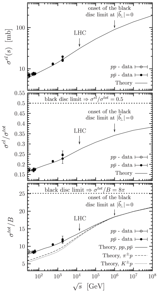
Figure 7.8: The elastic cross section $\sigma^{el}$ and the ratios $\sigma^{el}/\sigma^{tot}$ and $\sigma^{tot}/B$ as a function of the c.m. energy $\sqrt{s}$. The model results for $pp$ ($p{\bar{p}}$), $\pi p$, and $Kp$ scattering are represented by the solid, dashed and dotted lines, respectively. The experimental data for the $pp$ and $p{\bar{p}}$ reactions are indicated by the open and closed circles, respectively. The data for the elastic cross section are taken from [10] and the data for $\sigma^{tot}$ and $B$ from the references given in previous sections.

For $pp$ ($p{\bar{p}}$) scattering, we indicate explicitly the prediction for LHC at $\sqrt{s}=14\,\mbox{TeV}$ and the onset of the black disc limit at $\sqrt{s}=10^{6}\,\mbox{GeV}$. The model results for $\pi p$ and $Kp$ reactions are presented by the dashed and dotted line, respectively. For the ratios, the asymptotic limits are indicated: Since the maximum opacity or black disc limit governs the $\sqrt{s}\to\infty$ behavior, $\sigma^{el}/\sigma^{tot}$ ($\sigma^{tot}/B$) cannot exceed $0.5$ ($8\pi$) in hadron-hadron scattering.

In the investigation of $pp$ ($p{\bar{p}}$) scattering, our theoretical curves successfully confront the experimental data for the elastic cross section and both ratios. At low energies, the data are underestimated as reggeon contributions are not taken into account. Again, the agreement is comparable to the one achieved in [138] and better than in the approach of [57], where $\sigma^{el}$ comes out too small due to an underestimation of $d\sigma^{el}/dt$ in the low-$|t|$ region.

Concerning the energy dependence, $\sigma^{el}$ shows a similar behavior as $\sigma^{tot}$ but with a more pronounced flattening around $\sqrt{s}\gtrsim 10^{6}\,\mbox{GeV}$. This flattening is even stronger for the ratios, drawn on a linear scale, and reflects very clearly the onset of the black disc limit. As expected from the simple approximation (7.21), $\sigma^{el}/\sigma^{tot}$ and $\sigma^{tot}/B$ show a similar functional dependence on $\sqrt{s}$. At the highest energy shown, $\sqrt{s}=10^{8}\,\mbox{GeV}$, both ratios are still below the indicated asymptotic limits, which reflects that $J(s,|\vec{b}_{\!\perp}|)$ still deviates from the step-function shape (7.4). The ratios $\sigma^{el}/\sigma^{tot}$ and $\sigma^{tot}/B$ reach their upper limits $0.5$ and $8\pi$, respectively, at asymptotic energies, $\sqrt{s}\to\infty$, where the hadrons become infinitely large, completely black discs.

Comparing the $pp$ ($p{\bar{p}}$) results with the ones for $\pi p$ and $Kp$, one finds that the results for $\sigma^{tot}/B$ converge at high energies as shown in Fig. 7.8. This follows from the identical normalizations of the hadron wave functions that lead to an identical black disc limit for hadron-hadron reactions.

Chapter 8 Conclusion

We have developed a loop-loop correlation model (LLCM) [22, 23] in which the QCD vacuum is described by perturbative gluon exchange and the non-perturbative stochastic vacuum model (SVM) [27]. This combination leads to a static quark-antiquark potential with color Coulomb behavior for small and confining linear rise for large source separations in good agreement with lattice QCD results. We have computed in the LLCM the vacuum expectation value of one Wegner-Wilson loop, $\langle W_{r}[C]\rangle$, and the correlation of two Wegner-Wilson loops, $\langle W_{r_{1}}[C_{1}]W_{r_{2}}[C_{2}]\rangle$, for arbitrary loop geometries and general representations $r_{(i)}$ of $SU(N_{c})$. Specifying the loop geometries, these results allow us to compute the static quark-antiquark potential, the glueball mass, the chromo-field distributions of static color dipoles, the QCD van der Waals potential between two static color dipoles, and the $S$-matrix element for high-energy dipole-dipole scattering. Together with a phenomenological universal energy dependence and hadron and photon wave functions, the latter provides the basis for a unified description of hadron-hadron, photon-hadron, and photon-photon reactions within the functional integral approach to high-energy scattering.

We have applied the LLCM to compute the chromo-electric fields generated by a static color dipole in the fundamental and adjoint representation of $SU(N_{c})$. The formation of a confining color flux tube is described by the non-perturbative SVM correlations [28] and the color Coulomb field is obtained from perturbative gluon exchange. We have found Casimir scaling for both the perturbative and non-perturbative contributions to the chromo-electric fields in agreement with recent lattice data [84]. String breaking is neither described for sources in the fundamental representation nor for sources in the adjoint representation which indicates that in our approach not only dynamical fermions (quenched approximation) are missing but also some gluon dynamics. Transverse and longitudinal energy density profiles have been provided: For small dipoles, $R=0.1\,\mbox{fm}$, perturbative physics dominates and non-perturbative correlations are negligible. For large dipoles, $R\gtrsim 1\,\mbox{fm}$, the non-perturbative confining string dominates the chromo-electric fields between the color sources. The transition from perturbative to string behavior takes place at source separations of about $0.5\,\mbox{fm}$ in agreement with the recent results of Lüscher and Weisz [40]. The root mean squared radius $R_{ms}$ of the confining string and the energy density in the center of a fundamental $SU(3)$ dipole $\varepsilon_{3}(X=0)$ are governed completely by non-perturbative physics for large $R$ and saturate as $R$ increases at $R_{ms}^{R\to\infty}\approx 0.55\,\mbox{fm}$ and $\varepsilon_{3}^{R\to\infty}(X=0)\approx 1\,\mbox{GeV}/\mbox{fm}^{3}$.

We have presented the low-energy theorems [42, 43, 44], known in lattice QCD as Michael sum rules [41], in their complete form in continuum theory taking into account the contributions found in [29, 42] that are missing in the original formulation [41]. We have used the complete theorems to compare the energy and action stored in the confining string with the confining part of the static quark-antiquark potential. The comparison shows consistency of the model results and indicates that the non-perturbative SVM component is working at the renormalization scale at which $\beta(g)/g=-2$ and $\alpha_{s}=0.81$. Earlier SVM investigations along these lines have found a different value of $\alpha_{s}=0.57$ with the pyramid mantle choice for the surface [28, 29] but were incomplete since only the contribution from the traceless part of the energy-momentum tensor has been considered in the energy sum.

A Euclidean approach to high-energy dipole-dipole scattering has been established by generalizing Meggiolaro’s analytic continuation [45] from parton-parton scattering to gauge-invariant dipole-dipole scattering. The generalized analytic continuation allows us to derive $S$-matrix elements for high-energy reactions from configurations of Wegner-Wilson loops in Euclidean space-time with Euclidean functional integrals. It thus shows how one can access high-energy reactions directly in lattice QCD. First attempts in this direction have already been carried out but only very few signals could be extracted, while most of the data was dominated by noise [49]. We have applied this approach to compute in the Euclidean LLCM the scattering of dipoles at high-energy. The result derived in the Minkowskian version of the LLCM [23] has exactly been recovered including the well-known two-gluon exchange contribution to dipole-dipole scattering [99, 100]. This confirms the analytic continuation of the gluon field strength correlator used in all earlier applications of the SVM to high-energy scattering [30, 31, 32, 50, 51, 52, 53, 54, 55, 56, 57, 59, 60, 61, 58].

The $S$-matrix element obtained in our approach allows us to investigate manifestations of the confining QCD string in high-energy reactions of photons and hadrons [24] but leads to energy-independent cross sections in contradiction to the experimental observation [23]. The missing energy dependence is disappointing but not surprising since our approach does not describe explicit gluon radiation needed for a non-trivial energy dependence.

We have introduced a phenomenological energy dependence into the $S$-matrix element $S_{DD}$ that allows a unified description of hadron-hadron, photon-hadron, and photon-photon reactions and respects $S$-matrix unitarity constraints in impact parameter space [23, 25, 26]. Motivated by the two-pomeron model of Donnachie and Landshoff [62], we have ascribed to the non-perturbative and to the perturbative component a weak and a strong energy dependence, respectively. The constructed $T$-matrix element shows Regge behavior at moderately high energies and describes multiple gluonic interactions important to respect unitarity constraints in impact parameter space at ultra-high energies. However, for a more fundamental understanding of hadronic high-energy reactions in our model, one faces the highly ambitious task to implement gluon radiation and quantum evolution explicitly.

The model parameters have been adjusted to reproduce a wealth of experimental data (including cosmic ray data) for total, differential, and elastic cross sections, structure functions, and slope parameters over a large range of c.m. energies. The model parameters that allowed a good fit to high-energy scattering data are in good agreement with complementary investigations: The parameters of the non-perturbative component – the correlation length $a$, the non-Abelian strength $\kappa$, and the gluon condensate $G_{2}$ – are constrained by lattice QCD investigations, by the string tension $\sigma$ of a static quark-antiquark pair, and by the SVZ gluon condensate $G_{2}$ essential in QCD sum rule investigations. For the energy dependence, the exponents of the Donnachie-Landshoff two-pomeron fit, $\epsilon_{\mathrm{soft}}$ and $\epsilon_{\mathrm{hard}}$, have been used as an orientation for our energy exponents $\epsilon^{N\!P}$ and $\epsilon^{P}$. Besides these parameters describing dipole-dipole scattering, the reaction-dependent parameters in the light-cone wave functions are also consistent with other approaches: In the hadron wave functions, the transverse extension parameters $S_{h}$ are in good agreement with the corresponding electromagnetic radii [61] and the width of the longitudinal quark momentum distributions $\Delta z_{h}$ has been computed from [106]. In the photon wave function, the running quark masses, which coincide with the current quark masses for large $Q^{2}$ and the constituent quark masses for small $Q^{2}$ [52], have been chosen in agreement with sum rule derivations.

Having adjusted the model parameters, we have studied $S$-matrix unitarity limits of the scattering amplitudes in impact parameter space. On the basis of dipole-dipole scattering, we have shown explicitly that our model respects unitarity constraints in impact parameter space and, in particular, the black disc limit at ultra-high energies. The profile functions have been calculated for proton-proton and longitudinal photon-proton scattering. They show very clearly that the interacting particles become blacker and larger with increasing c.m. energy. At ultra-high energies, the opacity saturates at the black disc limit while the transverse expansion of the scattered particles continues. Increasing the photon virtuality $Q^{2}$ in longitudinal photon-proton scattering, the maximum opacity increases and also the energy at which it is reached for zero impact parameter.

We have related the impact parameter dependent gluon distribution $xG(x,Q^{2},|\vec{b}_{\perp}|)$ to the profile function for longitudinal photon-proton scattering and found low-$x$ saturation of $xG(x,Q^{2},|\vec{b}_{\perp}|)$ as a manifestation of $S$-matrix unitarity. In accordance with the profile function, $xG(x,Q^{2},|\vec{b}_{\perp}|)$ decreases from the center towards the periphery of the proton. With increasing photon virtuality $Q^{2}$, the increase of $xG(x,Q^{2},|\vec{b}_{\perp}|=0)$ becomes stronger towards small $x$ and the saturation value of $xG(x,Q^{2},|\vec{b}_{\perp}|=0)$ increases but is reached at decreasing values of $x$. However, the integrated gluon distribution $xG(x,Q^{2})$ does not saturate because of the growth of the proton radius with decreasing $x$ observed in our approach. Similar results are obtained in complementary approaches [124, 127, 128].

More model dependent are the specific energies at which these saturation effects set in. The profile function saturates the black disc limit at zero impact parameter for $\sqrt{s}\gtrsim 10^{6}\,\mbox{GeV}$ in proton-proton scattering and for $\sqrt{s}\gtrsim 10^{7}\,\mbox{GeV}$ in longitudinal photon-proton scattering with $Q^{2}\gtrsim 1\,\mbox{GeV}^{2}$. In both reactions, the wave function normalization determines the maximum opacity. The saturation of $xG(x,Q^{2},|\vec{b}_{\perp}|)$ occurs in our approach for $Q^{2}\gtrsim 1\,\mbox{GeV}^{2}$ at values of $x\lesssim 10^{-10}$, i.e. far below the HERA and THERA range.

For proton-proton scattering, we have found that the rise of the total and elastic cross section becomes weaker for $\sqrt{s}\gtrsim 10^{6}\,\mbox{GeV}$ due to the onset of the black disc limit at $|\vec{b}_{\perp}|=0$ in the profile function. This saturation of the profile function becomes even more apparent in the ratios $\sigma^{el}/\sigma^{tot}$ and $\sigma^{tot}/B$ which are a measure of the proton opacity. In contrast, no saturation effect has been observed in the slope parameter $B(s)$ which is a measure for the transverse expansion of the proton. Considering the differential elastic cross section $d\sigma^{el}/dt$, the model has described the diffraction pattern and also the shrinkage of the diffraction peak with increasing energy in good agreement with experimental data at small momentum transfers $|t|$. Around the dip region, where a real part is expected to be important, deviations from the data have reflected that our $T$-matrix is purely imaginary. Our predictions for proton-proton scattering at LHC ($\sqrt{s}=14\,\mbox{TeV}$) are a total cross section of $\sigma^{tot}_{pp}=114.2\,\mbox{mb}$ in good agreement with cosmic ray data and a differential elastic cross section $d\sigma^{el}/dt$ with a slope parameter of $B=21.26\,\mbox{GeV}^{-2}$, a negative curvature $C<0$, and a dip at $|t|\approx 0.35\,\mbox{GeV}^{2}$.

For pion-proton and kaon-proton scattering, results analogous to proton-proton scattering have been obtained but with a slightly stronger rise observed in the total cross section. This has been traced back to the smaller size of pions and kaons in comparison to protons, $S_{p}=0.86\,\mbox{fm}>S_{\pi}=0.607\,\mbox{fm}>S_{K}=0.55\,\mbox{fm}$, and the perturbative component becoming increasingly important with decreasing dipole sizes involved. Furthermore, a weak convergence of the ratios $\sigma^{tot}_{pp}/\sigma^{tot}_{\pi p}$ and $\sigma^{tot}_{pp}/\sigma^{tot}_{Kp}$ towards unity is predicted as the energy increases. The smaller size of the pion and kaon is reflected in the differential elastic cross sections $d\sigma^{el}/dt$ by the dip shifted towards larger values of $|t|$.

For photon-proton and photon-photon reactions, an even stronger rise of the total cross section has been observed with increasing energy. As illustrated in the proton structure function $F_{2}(x,Q^{2})$, this rise becomes steeper with increasing photon virtuality $Q^{2}$. Again, we have traced back the strong energy boost to the growing importance of the perturbative component with decreasing dipole size. Besides some deviations from the experimental data with increasing $Q^{2}$, our model has described $\sigma^{tot}_{\gamma^{*}p}(s,Q^{2})$ successfully in the low-$Q^{2}$ region where the running quark masses become constituent quark masses.

Finally, let us emphasize that the presented Euclidean approach to high-energy scattering is independent of our specific loop-loop correlation model. It indeed makes any method limited to a Euclidean formulation of the theory applicable for investigations of high-energy reactions. Here encouraging new results have been obtained with instantons [48] and within the AdS/CFT correspondence [46] and it will be interesting to see precise results from the lattice. A promising complementary Euclidean approach has been proposed in [160] where the structure functions of deep inelastic scattering at small Bjorken $x$ are related to an effective Euclidean field theory. Here one hopes that the limit $x\to 0$ corresponds to critical behavior in the effective theory. The aim is again to provide a framework in which structure functions can be calculated from first principles using genuine non-perturbative methods such as lattice computations. In another recent attempt, the energy dependence of the proton structure function has been related successfully to critical properties of an effective near light-cone Hamiltonian in a non-perturbative lattice approach [161]. It will be interesting to see further developments along these lines aiming at an understanding of hadronic high-energy scattering from the QCD Lagrangian.

Appendix A Loop and Minimal Surface Parametrizations

A rectangular loop $C_{i}$ with “spatial” extension $R_{i}$ and “temporal” extension $T_{i}$ placed in four-dimensional Euclidean space — as shown in Fig. A.1 — has the following parameter representation

$$C_{i}\,\,=\,\,C_{i}^{A}\,\cup\,C_{i}^{B}\,\cup\,C_{i}^{C}\,\cup\,C_{i}^{D}$$ (A.1)

with

$$C_{i}^{A}\,\,=\,\,\Big{\{}X_{i}^{A}(u_{i}) = X_{\!0\,i}-(1-z_{i})\,r_{i}+u_{i}\,t_{i},\quad\hphantom{v_{i}\,r_{i}}u_{i}\in[-T_{i},T_{i}]\Big{\}}$$ (A.2)

$$C_{i}^{B}\,\,=\,\,\Big{\{}X_{i}^{B}(v_{i}) = X_{\!0\,i}-(1-z_{i})\,r_{i}+v_{i}\,r_{i}+T_{i}\,t_{i},\;\quad v_{i}\in[0,1]\Big{\}}$$ (A.3)

$$C_{i}^{C}\,\,=\,\,\Big{\{}X_{i}^{C}(u_{i}) = X_{\!0\,i}+z_{i}\,r_{i}+u_{i}\,t_{i},\quad\hphantom{(1-z_{i})\,r_{i}}u_{i}\in[T_{i},-T_{i}]\Big{\}}$$ (A.4)

$$C_{i}^{D}\,\,=\,\,\Big{\{}X_{i}^{D}(v_{i}) = X_{\!0\,i}-(1-z_{i})\,r_{i}+v_{i}\,r_{i}+T_{i}\,t_{i},\;\quad v_{i}\in[1,0]\Big{\}}$$ (A.5)

where

$$r_{i}:=\left(\begin{array}[]{c}R_{i}\,\sin\theta_{i}\,\cos\phi_{i}\\ R_{i}\,\sin\theta_{i}\,\sin\phi_{i}\\ R_{i}\,\cos\theta_{i}\,\cos\Theta_{i}\\ R_{i}\,\cos\theta_{i}\,\sin\Theta_{i}\end{array}\right)\quad\mbox{and}\quad t_{i}:=\left(\!\!\begin{array}[]{c}0\\ 0\\ -\sin\Theta_{i}\\ \hphantom{-}\cos\Theta_{i}\end{array}\right)\ .$$ (A.6)

The “center” of the loop $C_{i}$ is given by $X_{\!0\,i}$. The parameters $z_{i}$, $R_{i}$, $\theta_{i}$, $\phi_{i}$, and $\Theta_{i}$ are defined in Fig. A.1 that illustrates (a) the spatial arrangement of a color dipole and (b) its world-line $C_{i}$ in Euclidean “longitudinal” space. The tilting angle $\Theta_{i}\neq 0$ is the central quantity in the analytic continuation presented in Chap. 4. Moreover, $\Theta_{1}=\pi/2$ together with $\Theta_{2}=0$ allows us to compute conveniently the chromo-magnetic field distributions in Appendix B.

The minimal surface $S_{i}$ is the planar surface bounded by the loop $C_{i}=\partial S_{i}$ given in (A.1). It can be parametrized as follows

$$S_{i}=\Big{\{}X_{i}(u_{i},v_{i})=X_{\!0\,i}-(1-z_{i})\,r_{i}+v_{i}\,r_{i}+u_{i}\,t_{i},\;u_{i}\in[-T_{i},T_{i}],\;v_{i}\in[0,1]\Big{\}}$$ (A.7)

with $r_{i}$ and $t_{i}$ given in (A.6). The corresponding infinitesimal surface element reads

$$d\sigma_{\mu\nu}(X_{i})=\Bigg{(}\frac{\partial X_{\!i\mu}}{\partial u_{i}}\frac{\partial X_{\!i\nu}}{\partial v_{i}}-\frac{\partial X_{\!i\mu}}{\partial v_{i}}\frac{\partial X_{\!i\nu}}{\partial u_{i}}\Bigg{)}\,du_{i}\,dv_{i}=\Bigg{(}t_{i\mu}r_{i\nu}-r_{i\mu}t_{i\nu}\Bigg{)}\,du_{i}\,dv_{i}\ .$$ (A.8)

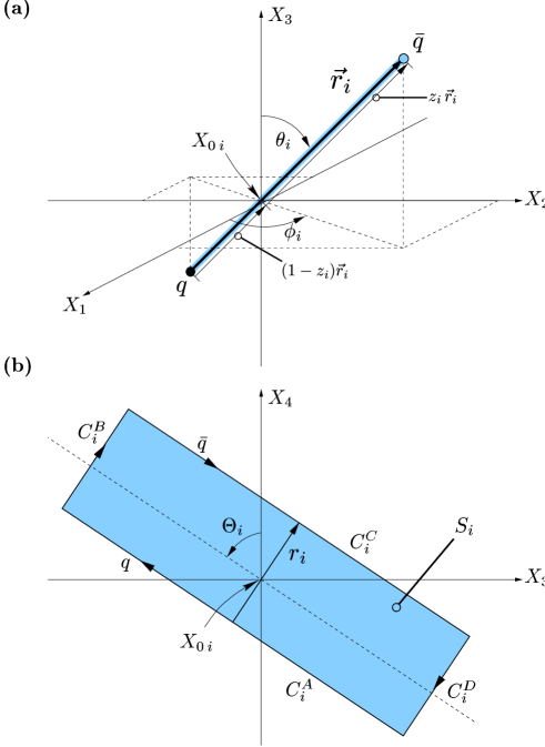
Figure A.1: (a) Spatial arrangement of a color dipole and (b) its world-line in Euclidean “longitudinal” space given by the rectangular loop $C_{i}$ that defines the minimal surface $S_{i}$ with $\partial S_{i}=C_{i}$. The minimal surface is represented by the shaded area. In our model, it is interpreted as the world-sheet of the QCD string that confines the quark and antiquark in the dipole.

Appendix B $\chi$-Computations with Minimal Surfaces

The quantities considered in the main text are computed from the VEV of one loop $\langle W[C]\rangle$ and the loop-loop correlation function $\langle W[C_{1}]W[C_{2}]\rangle$. Using the Gaussian approximation in the gluon field strengths, both are expressed in terms of $\chi_{S_{i}S_{j}}$-functions (2.15) and (2.27) as shown in Secs. 2.1 and 2.2. These $\chi$-functions are central quantities since here the ansatz of the gauge-invariant bilocal gluon field strength correlator and the surface choice enter the model. In this Appendix these functions are computed explicitly for minimal surfaces (A.7) and the $F_{\mu\nu\rho\sigma}$ - ansatz given in (2.42), (2.3), and (2.3). Note that the contributions from the infinitesimally thin tube — which allows us to compare the gluon field strengths in surface $S_{1}$ with the gluon field strength in surface $S_{2}$ — cancel mutually.

Depending on the geometries and the relative arrangement of the loops, the $\chi$-functions determine the physical quantities investigated within the LLCM such as the static $q{\bar{q}}$ potential (3.2), the chromo-field distributions of a color dipole (3.21), and the $S$-matrix element for elastic dipole-dipole scattering (4.12).

We compute separately the three components $\chi_{S_{1}S_{2}}^{P}$, $\chi_{S_{1}S_{2}}^{N\!P\,nc}$, and $\chi_{S_{1}S_{2}}^{N\!P\,c}$ for general loop arrangements from which the considered quantities are obtained as special cases. Without loss of generality, the center of the loop $C_{2}$ is placed at the origin of the coordinate system, $X_{\!0\,2}=(0,0,0,0)$. Moreover, $C_{2}$ is kept untilted, $\Theta_{2}=0$, and $\Theta:=\Theta_{1}$ is used to simplify notation. We limit our general computation to loops with $r_{1,2}=(\vec{r}_{1,2\perp},0,0)\,\,\equiv\,\,\theta_{1,2}=\pi/2$ and transverse “impact parameters” $b=X_{\!0\,1}-X_{\!0\,2}=X_{\!0\,1}=(b_{1},b_{2},0,0)=(\vec{b}_{\!\perp},0,0)$ which allows to compute all of the considered quantities.

$\chi_{S_{1}S_{2}}^{N\!P\,c}$-Computation

Starting with the definition

$$\chi_{S_{1}S_{2}}^{N\!P\,c} := \frac{\pi^{2}}{4}\int_{S_{1}}\!\!d\sigma_{\mu\nu}(X_{1})\int_{S_{2}}\!\!d\sigma_{\rho\sigma}(X_{2})\,F_{\mu\nu\rho\sigma}^{N\!P\,c}(Z=X_{1}-X_{2})$$

$$= \frac{\pi^{2}G_{2}\kappa}{12(N_{c}^{2}-1)}\int_{S_{1}}\!\!d\sigma_{\mu\nu}(X_{1})\int_{S_{2}}\!\!d\sigma_{\rho\sigma}(X_{2})\left(\delta_{\mu\rho}\delta_{\nu\sigma}-\delta_{\mu\sigma}\delta_{\nu\rho}\right)D(Z^{2})\ ,$$

one exploits the anti-symmetry of the surface elements, $d\sigma_{\mu\nu}=-d\sigma_{\nu\mu}$, and applies the surface parametrization (A.7) with the corresponding surface elements (A.8) to obtain

$$\chi_{S_{1}S_{2}}^{N\!P\,c}=\cos\Theta\,\frac{\pi^{2}G_{2}\kappa}{3(N_{c}^{2}-1)}\,(r_{1}\cdot r_{2})\int_{0}^{1}\!\!dv_{1}\int_{0}^{1}\!\!dv_{2}\int_{-T_{1}}^{T_{1}}\!\!du_{1}\int_{-T_{2}}^{T_{2}}\!\!du_{2}\,D(Z^{2})$$ (B.2)

with

$$Z=X_{1}-X_{2}=\left(\begin{array}[]{l}\!\!\hphantom{-\,}\vec{b}_{\!\perp}-(1-z_{1})\,\vec{r}_{1\perp}+v_{1}\,\vec{r}_{1\perp}+(1-z_{2})\,\vec{r}_{2\perp}-v_{2}\,\vec{r}_{2\perp}\\ \!\!-\,u_{1}\sin\Theta\\ \!\!\hphantom{-\,}u_{1}\cos\Theta-u_{2}\end{array}\right)\ ,$$ (B.3)

where the identities $t_{1}\cdot r_{2}=r_{1}\cdot t_{2}=0$ and $t_{1}\cdot t_{2}=\cos\Theta$, evident from (A.6) with the mentioned specification of the loop geometries, have been used. In the limit $T_{2}\rightarrow\infty$, the $u_{2}$ integration can be performed

$$\lim_{T_{2}\to\infty}\int_{-T_{2}}^{T_{2}}\!\!du_{2}\,D(Z^{2})\,\,=\,\,\int\frac{d^{4}K}{(2\pi)^{4}}\,\tilde{D}(K^{2})\lim_{T_{2}\to\infty}\int_{-T_{2}}^{T_{2}}\!\!du_{2}\,e^{iKZ}$$

$$=\int\frac{d^{4}K}{(2\pi)^{4}}\,\tilde{D}(K^{2})\,2\pi\,\delta(K_{4})\,\exp\!\left[i\vec{K}_{\!\perp}\vec{Z}_{\!\perp}+iK_{3}u_{1}\sin\Theta+iK_{4}u_{1}\cos\Theta\right]$$

$$=\int\frac{d^{3}K}{(2\pi)^{3}}\,\tilde{D}^{(3)}(\vec{K}^{2})\,\exp\!\left[i\vec{K}_{\!\perp}\vec{Z}_{\!\perp}+iK_{3}u_{1}\sin\Theta\right]\,\,=\,\,D^{(3)}(\vec{Z}^{2})\ ,$$ (B.4)

which leads to

$$\lim_{T_{2}\to\infty}\chi_{S_{1}S_{2}}^{N\!P\,c}=\cos\Theta\,\frac{\pi^{2}G_{2}\kappa}{3(N_{c}^{2}-1)}\,(\vec{r}_{1\perp}\cdot\vec{r}_{2\perp})\int_{0}^{1}\!\!dv_{1}\int_{0}^{1}\!\!dv_{2}\int_{-T_{1}}^{T_{1}}\!\!du_{1}\,D^{(3)}(\vec{Z}^{2})\ .$$ (B.5)

Taking in addition the limit $T_{1}\rightarrow\infty$, the $u_{1}$ integration can be performed as well

$$\lim_{T_{1}\to\infty}\int_{-T_{1}}^{T_{1}}\!\!du_{1}e^{iK_{3}u_{1}\sin\Theta}=\left\{\begin{array}[]{lc}2\pi\delta(K_{3}\sin\Theta)=\frac{2\pi\delta(K_{3})}{|\sin\Theta|}&\quad\mbox{for}\quad\sin\Theta\neq 0\\ \lim_{T_{1}\to\infty}\,2\,T_{1}&\quad\mbox{for}\quad\sin\Theta=0\\ \end{array}\right.\ .$$ (B.6)

With $T_{1}=T_{2}=T/2\to\infty$, one obtains for $\sin\Theta\neq 0$

$$\lim_{T\to\infty}\chi_{S_{1}S_{2}}^{N\!P\,c}=\frac{\cos\Theta}{|\sin\Theta|}\,\frac{\pi^{2}G_{2}\kappa}{3(N_{c}^{2}-1)}\,(\vec{r}_{1\perp}\cdot\vec{r}_{2\perp})\int_{0}^{1}\!\!dv_{1}\int_{0}^{1}\!\!dv_{2}\,D^{(2)}(\vec{Z}_{\!\perp}^{2})$$ (B.7)

and for $\sin\Theta=0$

$$\lim_{T\to\infty}\chi_{S_{1}S_{2}}^{N\!P\,c}=\lim_{T\to\infty}\,T\,\cos\Theta\,\frac{\pi^{2}G_{2}\kappa}{3(N_{c}^{2}-1)}\,(\vec{r}_{1\perp}\cdot\vec{r}_{2\perp})\int_{0}^{1}\!\!dv_{1}\int_{0}^{1}\!\!dv_{2}\,D^{(3)}(\vec{Z}^{2})\ .$$ (B.8)

Evidently, (B.7) is the result given in (4.14) and (4.17) that describes the confining contribution to the dipole-dipole scattering matrix element $S_{DD}$.

From (B.8), one obtains the confining contribution to the static color dipole potential for $S_{1}=S_{2}=S$ which implies $T_{1}=T_{2}=T/2$, $\Theta=0$, $z_{1}=z_{2}$, $r_{1}=r_{2}=r$, and $\vec{r}_{1\perp}\cdot\vec{r}_{2\perp}=r^{2}=R^{2}$ so that

$$\lim_{T\to\infty}\chi_{SS}^{N\!P\,c} = \lim_{T\to\infty}\,T\,\frac{\pi^{2}G_{2}\kappa}{3(N_{c}^{2}-1)}\,R^{2}\int_{0}^{1}\!\!dv_{1}\int_{0}^{1}\!\!dv_{2}\,D^{(3)}(\vec{Z}^{2}=(v_{1}-v_{2})^{2}R^{2})$$ (B.9)

$$= \lim_{T\to\infty}\,T\,\frac{2\pi^{2}G_{2}\kappa}{3(N_{c}^{2}-1)}\,R^{2}\int_{0}^{1}\!\!d\rho\,(1-\rho)\,D^{(3)}(\rho^{2}R^{2})\ ,$$

which leads directly to (3.7).

From (B.5) the confining contribution to the chromo-field distributions $\Delta G_{\alpha\beta}^{2}(X)$ can be computed conveniently. Equation (B.5) reads for $S_{1}=S_{P}$, $T_{1}=R_{P}/2$ and $R_{1}=R_{P}$, and $S_{2}=S_{W}$, $T_{2}=T/2$ and $R_{2}=R$

$$\lim_{T\to\infty}\chi_{S_{P}S_{W}}^{N\!P\,c}=\cos\Theta\,\frac{\pi^{2}G_{2}\kappa}{3(N_{c}^{2}-1)}\,(\vec{r}_{1\perp}\cdot\vec{r}_{2\perp})\int_{0}^{1}\!\!dv_{1}\int_{0}^{1}\!\!dv_{2}\int_{-R_{P}/2}^{R_{P}/2}\!\!du_{1}\,D^{(3)}(\vec{Z}^{2})$$ (B.10)

with

$$\vec{Z}=\vec{X}_{1}-\vec{X}_{2}=\left(\begin{array}[]{l}\!\!\hphantom{-\,}\vec{b}_{\!\perp}-(1-z_{1})\,\vec{r}_{1\perp}+v_{1}\,\vec{r}_{1\perp}+(1-z_{2})\,\vec{r}_{2\perp}-v_{2}\,\vec{r}_{2\perp}\\ \!\!-\,u_{1}\sin\Theta\end{array}\right)\ .$$ (B.11)

The confining non-perturbative contribution to the chromo-magnetic fields vanishes as it is obtained for plaquettes with $\Theta=\pi/2$. The corresponding contribution to the chromo-electric fields can be computed with $\Theta=0$ as follows: Due to $R_{1}=R_{p}\to 0$, the $u_{1}$ and $v_{1}$ integrations in (B.10) can be performed with the mean value theorem. Keeping only terms up to ${\cal O}(R_{p}^{2})$, the confining non-perturbative contribution to the chromo-field distributions $\Delta G_{\alpha\beta}^{2}(X)$ is obtained as given in (3.30).

$\chi_{S_{1}S_{2}}^{N\!P\,nc}$-Computation

We start again with the definition

$$\chi_{S_{1}S_{2}}^{N\!P\,nc} := \frac{\pi^{2}}{4}\int_{S_{1}}\!\!d\sigma_{\mu\nu}(X_{1})\int_{S_{2}}\!\!d\sigma_{\rho\sigma}(X_{2})\,F_{\mu\nu\rho\sigma}^{N\!P\,nc}(Z=X_{1}-X_{2})$$

$$= \frac{\pi^{2}G_{2}(1\!-\!\kappa)}{12(N_{c}^{2}-1)}\,\int_{S_{1}}\!\!d\sigma_{\mu\nu}(X_{1})\int_{S_{2}}\!\!d\sigma_{\rho\sigma}(X_{2})$$

$$\times\frac{1}{2}\Bigl{[}\frac{\partial}{\partial Z_{\nu}}\left(Z_{\sigma}\delta_{\mu\rho}-Z_{\rho}\delta_{\mu\sigma}\right)+\frac{\partial}{\partial Z_{\mu}}\left(Z_{\rho}\delta_{\nu\sigma}-Z_{\sigma}\delta_{\nu\rho}\right)\Bigr{]}\,D_{1}(Z^{2})$$

and use the anti-symmetry of both surface elements to obtain

$$\!\!\!\!\!\!\!\!\!\!\!\!\!\!\!\!\!\!\chi_{S_{1}S_{2}}^{N\!P\,nc}\!\! = \frac{\pi^{2}G_{2}(1\!-\!\kappa)}{6(N_{c}^{2}-1)}\,\int_{S_{1}}\!\!d\sigma_{\mu\nu}(X_{1})\int_{S_{2}}\!\!d\sigma_{\rho\sigma}(X_{2})\,\frac{\partial}{\partial Z_{\nu}}\,Z_{\sigma}\,\delta_{\mu\rho}\,D_{1}(Z^{2})$$ (B.13)

$$= \frac{\pi^{2}G_{2}(1\!-\!\kappa)}{3(N_{c}^{2}-1)}\!\int_{S_{1}}\!\!d\sigma_{\mu\nu}(X_{1})\!\int_{S_{2}}\!\!d\sigma_{\rho\sigma}(X_{2})\,\frac{\partial}{\partial Z_{\nu}}\,\frac{\partial}{\partial Z_{\sigma}}\,\delta_{\mu\rho}\,D_{1}^{\prime}(Z^{2})$$ (B.14)

$$= \!\!\!\!-\,\frac{\pi^{2}G_{2}(1\!-\!\kappa)}{3(N_{c}^{2}-1)}\!\!\int_{S_{1}}\!\!\!d\sigma_{\mu\nu}(X_{1})\frac{\partial}{\partial X_{1\nu}}\!\int_{S_{2}}\!\!\!d\sigma_{\rho\sigma}(X_{2})\frac{\partial}{\partial X_{2\sigma}}\,\delta_{\mu\rho}\,D_{1}^{\prime}(Z^{2})$$ (B.15)

with

$$D_{1}^{\prime}(Z^{2})=\int\!\!\frac{d^{4}K}{(2\pi)^{4}}\,e^{iKZ}\,\tilde{D}_{1}^{\prime}(K^{2})=\int\!\!\frac{d^{4}K}{(2\pi)^{4}}\,e^{iKZ}\,\frac{d}{dK^{2}}\,\tilde{D}_{1}(K^{2})\ .$$ (B.16)

As evident from (B.15), Stokes’ theorem can be used to transform each of the surface integrals in $\chi_{S_{1}S_{2}}^{N\!P\,nc}$ into a line integral

$$\chi_{S_{1}S_{2}}^{N\!P\,nc}\!\! = -\,\frac{\pi^{2}G_{2}(1\!-\!\kappa)}{3(N_{c}^{2}-1)}\int_{S_{1}}\!\!\!d\sigma_{\mu\nu}(X_{1})\frac{\partial}{\partial Z_{\nu}}\!\oint_{C_{2}}\!\!\!dZ_{\rho}(X_{2})\,\delta_{\mu\rho}\,D_{1}^{\prime}(Z^{2})$$ (B.17)

$$= -\,\frac{\pi^{2}G_{2}(1\!-\!\kappa)}{6(N_{c}^{2}-1)}\int_{S_{1}}\!\!\!d\sigma_{\mu\nu}(X_{1})\!\oint_{C_{2}}\!\!\!dZ_{\rho}(X_{2})\,\delta_{\mu\rho}\,Z_{\nu}\,D_{1}(Z^{2})$$ (B.18)

$$= -\,\frac{\pi^{2}G_{2}(1\!-\!\kappa)}{3(N_{c}^{2}-1)}\,\oint_{C_{1}}\!\!\!dZ_{\mu}(X_{1})\oint_{C_{2}}\!\!\!dZ_{\rho}(X_{2})\,\delta_{\mu\rho}\,D_{1}^{\prime}(Z^{2})\ .$$ (B.19)

With the line parametrizations of $C_{1}$ and $C_{2}$ given in (A.1) and the specification of the loop geometries mentioned at the beginning of this appendix, (B.19) becomes

$$\!\!\!\!\!\!\!\!\chi_{S_{1}S_{2}}^{N\!P\,nc}=-\,\frac{\pi^{2}G_{2}(1-\kappa)}{3(N_{c}^{2}-1)}$$ (B.20)

$$\!\!\!\!\!\!\!\!\times\Bigg{\{}\cos\Theta\!\!\int_{-T_{1}}^{T_{1}}\!\!\!du_{1}\!\!\int_{-T_{2}}^{T_{2}}\!\!\!du_{2}\Big{[}D_{1}^{\prime}(Z_{AA}^{2})\!-\!D_{1}^{\prime}(Z_{AC}^{2})\!-\!D_{1}^{\prime}(Z_{CA}^{2})\!+\!D_{1}^{\prime}(Z_{CC}^{2})\Big{]}$$

$$\!\!\!\!\!\!+\,(\vec{r}_{1\perp}\cdot\vec{r}_{2\perp})\!\!\int_{0}^{1}\!\!\!dv_{1}\!\!\int_{0}^{1}\!\!\!dv_{2}\Big{[}D_{1}^{\prime}(Z_{BB}^{2})\!-\!D_{1}^{\prime}(Z_{BD}^{2})\!-\!D_{1}^{\prime}(Z_{DB}^{2})\!+\!D_{1}^{\prime}(Z_{DD}^{2})\Big{]}\Bigg{\}}$$

where the following shorthand notation is used

$$Z_{XY}:=X_{1}^{X}-X_{2}^{Y}\quad\mbox{with}\quad X_{2}^{X}\in C_{2}^{X}\quad\mbox{and}\quad X_{2}^{Y}\in C_{2}^{Y}\ .$$ (B.21)

In the limit $R_{1,2}\ll T_{1,2}\to\infty$, the term $\propto\!(\vec{r}_{1\perp}\cdot\vec{r}_{2\perp})$ on the rhs of (B.20) can be neglected and, thus, (B.20) reduces to

$$\lim_{T_{1}\to\infty\atop T_{2}\to\infty}\chi_{S_{1}S_{2}}^{N\!P\,nc}=-\,\cos\Theta\,\frac{\pi^{2}G_{2}(1-\kappa)}{3(N_{c}^{2}-1)}\,\lim_{T_{1}\to\infty}\int_{-T_{1}}^{T_{1}}\!\!du_{1}\lim_{T_{2}\to\infty}\int_{-T_{2}}^{T_{2}}\!\!du_{2}$$ (B.22)

$$\hskip 71.13188pt\times\Big{[}D_{1}^{\prime}(Z_{AA}^{2})-D_{1}^{\prime}(Z_{AC}^{2})-D_{1}^{\prime}(Z_{CA}^{2})+D_{1}^{\prime}(Z_{CC}^{2})\Big{]}\ .$$

Here the integrations over $u_{1}$ and $u_{2}$ can be performed analytically proceeding analogously to (B.4) and (B.6). With $T_{1}=T_{2}=T/2\to\infty$, one obtains for $\sin\Theta\neq 0$

$$\!\!\!\!\!\!\lim_{T\to\infty}\chi_{S_{1}S_{2}}^{N\!P\,nc}=-\,\frac{\cos\Theta}{|\sin\Theta|}\,\frac{\pi^{2}G_{2}(1-\kappa)}{3(N_{c}^{2}-1)}\,$$ (B.23)

$$\!\!\!\!\!\!\hskip 14.22636pt\times\Big{[}D_{1}^{\prime\,(2)}(\vec{Z}_{AA\perp}^{2})-D_{1}^{\prime\,(2)}(\vec{Z}_{AC\perp}^{2})-D_{1}^{\prime\,(2)}(\vec{Z}_{CA\perp}^{2})+D_{1}^{\prime\,(2)}(\vec{Z}_{CC\perp}^{2})\Big{]}$$

and for $\sin\Theta=0$

$$\!\!\!\!\!\!\lim_{T\to\infty}\chi_{S_{1}S_{2}}^{N\!P\,nc}=-\,\lim_{T\to\infty}T\,\cos\Theta\,\frac{\pi^{2}G_{2}(1-\kappa)}{3(N_{c}^{2}-1)}\,$$ (B.24)

$$\!\!\!\!\!\!\hskip 14.22636pt\times\Big{[}D_{1}^{\prime\,(3)}(\vec{Z}_{AA}^{2})-D_{1}^{\prime\,(3)}(\vec{Z}_{AC}^{2})-D_{1}^{\prime\,(3)}(\vec{Z}_{CA}^{2})+D_{1}^{\prime\,(3)}(\vec{Z}_{CC}^{2})\Big{]}\ .$$

With the following identities

$$\vec{Z}_{AA\perp}=\vec{r}_{1q}-\vec{r}_{2q}\ ,\,\,\,\,\vec{Z}_{AC\perp}=\vec{r}_{1q}-\vec{r}_{2{\bar{q}}}\ ,\,\,\,\,\vec{Z}_{CA\perp}=\vec{r}_{1{\bar{q}}}-\vec{r}_{2q}\ ,\,\,\,\,\vec{Z}_{CC\perp}=\vec{r}_{1{\bar{q}}}-\vec{r}_{2{\bar{q}}}\ ,\,\,\,\,$$ (B.25)

one sees immediately that (B.23) is the result given in (4.14) and (4.16) that describes the non-confining non-perturbative contribution to the dipole-dipole scattering matrix element $S_{DD}$.

From (B.24) one obtains the non-confining contribution to the static potential for $S_{1}=S_{2}=S$, i.e., $T_{1}=T_{2}=T/2$, $\Theta=0$, $r_{1}=r_{2}=r$,

$$\!\!\!\!\!\!\lim_{T\to\infty}\chi_{SS}^{N\!P\,nc}=-\,\lim_{T\to\infty}T\,\,\frac{\pi^{2}G_{2}(1-\kappa)}{3(N_{c}^{2}-1)}\,\,$$ (B.26)

$$\!\!\!\!\!\!\hskip 14.22636pt\times\Big{[}D_{1}^{\prime\,(3)}(\vec{Z}_{AA}^{2})-D_{1}^{\prime\,(3)}(Z_{AC}^{2})-D_{1}^{\prime\,(3)}(\vec{Z}_{CA}^{2})+D_{1}^{\prime\,(3)}(\vec{Z}_{CC}^{2})\Big{]}\ ,$$

which contributes to the self-energy of the color sources with

$$\lim_{T\to\infty}\chi_{SS\,\mbox{\scriptsize self}}^{N\!P\,nc} = -\,\lim_{T\to\infty}T\,\,\frac{\pi^{2}G_{2}(1-\kappa)}{3(N_{c}^{2}-1)}\,\,\Big{[}D_{1}^{\prime\,(3)}(\vec{Z}_{AA}^{2})+D_{1}^{\prime\,(3)}(\vec{Z}_{CC}^{2})\Big{]}$$ (B.27)

$$= -\,\lim_{T\to\infty}T\,\,\frac{2\pi^{2}G_{2}(1-\kappa)}{3(N_{c}^{2}-1)}\,\,D_{1}^{\prime\,(3)}(\vec{Z}_{AA}^{2})$$

and to the potential energy between the color sources with

$$\lim_{T\to\infty}\chi_{SS\,\mbox{\scriptsize pot}}^{N\!P\,nc} = \lim_{T\to\infty}T\,\,\frac{\pi^{2}G_{2}(1-\kappa)}{6(N_{c}^{2}-1)}\,\,\Big{[}D_{1}^{\prime\,(3)}(\vec{Z}_{AC}^{2})+D_{1}^{\prime\,(3)}(\vec{Z}_{CA}^{2})\Big{]}$$ (B.28)

$$= \lim_{T\to\infty}T\,\,\frac{\pi^{2}G_{2}(1-\kappa)}{3(N_{c}^{2}-1)}\,\,D_{1}^{\prime\,(3)}(\vec{Z}_{AC}^{2})\ .$$

The latter gives the non-confining contribution to the static potential (3.6).

From (B.18) the non-confining non-perturbative contribution to the chromo-electric fields ($\Delta G_{\alpha\beta}^{2}(X)$ with $\alpha\beta=i4=4i$) can be computed most conveniently with zero plaquette tilting angle $\Theta=0$. The corresponding contribution to the chromo-magnetic fields ($\Delta G_{\alpha\beta}^{2}(X)$ with $\alpha\beta=ij=ji$) is obtained for plaquette tilting angle $\Theta=\pi/2$ and thus vanishes which can be seen most directly from the surface integrals (B.13). Now, we set $\Theta=0$ to compute the contribution to the chromo-electric fields: Using the surface $S_{1}=S_{P}$ and loop $C_{2}=\partial S_{W}$ parametrizations, (A.7) and (A.1), with our specification of the loop geometries, one obtains from (B.18)

$$\chi_{S_{P}S_{W}}^{N\!P\,nc}\!\! = -\,\frac{\pi^{2}G_{2}(1\!-\!\kappa)}{3(N_{c}^{2}-1)}\int_{-R_{P}/2}^{R_{P}/2}\!\!du_{1}\int_{0}^{1}\!\!dv_{1}$$

$$\times\left\{\int_{-T/2}^{T/2}\!\!du_{2}\,\left[(\vec{r}_{1\perp}\cdot\vec{Z}_{1A\perp})\,D_{1}(Z_{1A}^{2})-(\vec{r}_{1\perp}\cdot\vec{Z}_{1C\perp})\,D_{1}(Z_{1C}^{2})\right]\right.$$

$$\hphantom{\times\,}\left.-\,(\vec{r}_{1\perp}\cdot\vec{r}_{2\perp})\int_{0}^{1}\!\!dv_{2}\,\left[(\vec{r}_{1\perp}\cdot\vec{Z}_{1B\perp})\,D_{1}(Z_{1B}^{2})-(\vec{r}_{1\perp}\cdot\vec{Z}_{1D\perp})\,D_{1}(Z_{1D}^{2})\right]\right\}$$

with $T_{1}=R_{P}/2$, $R_{1}=R_{P}$, $T_{2}=T/2$, $R_{2}=R$, and the shorthand notation

$$Z_{1X}:=X_{1}-X_{2}^{X}\quad\mbox{with}\quad X_{1}\in S_{1}=S_{P}\quad\mbox{and}\quad X_{2}^{X}\in C_{2}^{X}=\partial S_{W}^{X}\ .$$ (B.30)

In the limit $R\ll T\to\infty$, the term $\propto\!(\vec{r}_{1\perp}\cdot\vec{r}_{2\perp})$ on the rhs of (B) can be neglected

$$\lim_{T\to\infty}\chi_{S_{P}S_{W}}^{N\!P\,nc}\!\! = -\,\frac{\pi^{2}G_{2}(1\!-\!\kappa)}{3(N_{c}^{2}-1)}\int_{-R_{P}/2}^{R_{P}/2}\!\!du_{1}\int_{0}^{1}\!\!dv_{1}\lim_{T\to\infty}\int_{-T/2}^{T/2}\!\!du_{2}\,$$

$$\times\left[(\vec{r}_{1\perp}\cdot\vec{Z}_{1A\perp})\,D_{1}(Z_{1A}^{2})-(\vec{r}_{1\perp}\cdot\vec{Z}_{1C\perp})\,D_{1}(Z_{1C}^{2})\right]\ .$$

With an infinitesimal plaquette used to measure the chromo-electric field, $R_{1}=R_{p}\to 0$, the mean value theorem can be used to perform the $u_{1}$ and $v_{1}$ integrations in (B). Keeping only terms up to ${\cal O}(R_{p}^{2})$, this leads directly to the non-confining non-perturbative contribution to the chromo-field distributions $\Delta G_{\alpha\beta}^{2}(X)$ as given in (3.28) and (3.29).

$\chi^{P}$-Computation

Comparing the definition of the perturbative component

$$\chi_{S_{1}S_{2}}^{P} := \frac{\pi^{2}}{4}\int_{S_{1}}\!\!d\sigma_{\mu\nu}(X_{1})\int_{S_{2}}\!\!d\sigma_{\rho\sigma}(X_{2})\,F_{\mu\nu\rho\sigma}^{P}(Z=X_{1}-X_{2})$$

$$= \frac{g^{2}}{4}\,\int_{S_{1}}\!\!d\sigma_{\mu\nu}(X_{1})\int_{S_{2}}\!\!d\sigma_{\rho\sigma}(X_{2})$$

$$\times\frac{1}{2}\Bigl{[}\frac{\partial}{\partial Z_{\nu}}\left(Z_{\sigma}\delta_{\mu\rho}-Z_{\rho}\delta_{\mu\sigma}\right)+\frac{\partial}{\partial Z_{\mu}}\left(Z_{\rho}\delta_{\nu\sigma}-Z_{\sigma}\delta_{\nu\rho}\right)\Bigr{]}\,D_{P}(Z^{2})$$

with the one of the non-confining non-perturbative component $\chi_{S_{1}S_{2}}^{N\!P\,nc}$ given in (B), one finds an identical structure. Thus, accounting for the different prefactors and the different correlation function, the results for $\chi_{S_{1}S_{2}}^{P}$ can be read off directly from the results for $\chi_{S_{1}S_{2}}^{N\!P\,nc}$ given above:

With $T_{1}=T_{2}=T/2\to\infty$ and our specification of the loop geometries, one obtains the result for $\sin\Theta\neq 0$ from (B.23)

$$\!\!\!\!\!\!\lim_{T\to\infty}\chi_{S_{1}S_{2}}^{P}=-\,\frac{\cos\Theta}{|\sin\Theta|}\,g^{2}\,$$ (B.33)

$$\!\!\!\!\!\!\hskip 14.22636pt\times\Big{[}D_{P}^{\prime\,(2)}(\vec{Z}_{AA\perp}^{2})-D_{P}^{\prime\,(2)}(Z_{AC\perp}^{2})-D_{P}^{\prime\,(2)}(\vec{Z}_{CA\perp}^{2})+D_{P}^{\prime\,(2)}(\vec{Z}_{CC\perp}^{2})\Big{]}$$

and the result for $\sin\Theta=0$ from (B.24)

$$\!\!\!\!\!\!\lim_{T\to\infty}\chi_{S_{1}S_{2}}^{P}=-\,\lim_{T\to\infty}T\,\cos\Theta\,g^{2}\,$$ (B.34)

$$\!\!\!\!\!\!\hskip 14.22636pt\times\Big{[}D_{P}^{\prime\,(3)}(\vec{Z}_{AA}^{2})-D_{P}^{\prime\,(3)}(Z_{AC}^{2})-D_{P}^{\prime\,(3)}(\vec{Z}_{CA}^{2})+D_{P}^{\prime\,(3)}(\vec{Z}_{CC}^{2})\Big{]}\ ,$$

where $Z_{XY}$ is defined in (B.21) and $Z_{XY\perp}$ is given explicitly in (B.25). Evidently, (B.33) is the final result given in (4.14) and (4.15) that describes the perturbative contribution the dipole-dipole scattering matrix element $S_{DD}$.

The perturbative contribution to the static potential is obtained from the expression corresponding to (B.26),

$$\!\!\!\!\!\!\lim_{T\to\infty}\chi_{SS}^{P}=-\,\lim_{T\to\infty}T\,\,g^{2}\,\,$$ (B.35)

$$\!\!\!\!\!\!\hskip 14.22636pt\times\Big{[}D_{P}^{\prime\,(3)}(\vec{Z}_{AA}^{2})-D_{P}^{\prime\,(3)}(Z_{AC}^{2})-D_{P}^{\prime\,(3)}(\vec{Z}_{CA}^{2})+D_{P}^{\prime\,(3)}(\vec{Z}_{CC}^{2})\Big{]}\ ,$$

which contributes to the self-energy of the color sources with

$$\lim_{T\to\infty}\chi_{SS\,\mbox{\scriptsize self}}^{P} = -\,\lim_{T\to\infty}T\,\,g^{2}\,\,\Big{[}D_{P}^{\prime\,(3)}(\vec{Z}_{AA}^{2})+D_{P}^{\prime\,(3)}(\vec{Z}_{CC}^{2})\Big{]}$$ (B.36)

$$= -\,\lim_{T\to\infty}T\,\,2\,g^{2}\,\,D_{P}^{\prime\,(3)}(\vec{Z}_{AA}^{2})$$

and to the potential energy between the color sources with

$$\lim_{T\to\infty}\chi_{SS\,\mbox{\scriptsize pot}}^{P} = -\,\lim_{T\to\infty}T\,\,g^{2}\,\,\Big{[}D_{P}^{\prime\,(3)}(\vec{Z}_{AC}^{2})+D_{P}^{\prime\,(3)}(\vec{Z}_{CA}^{2})\Big{]}$$ (B.37)

$$= -\,\lim_{T\to\infty}T\,\,2\,g^{2}\,\,D_{P}^{\prime\,(3)}(\vec{Z}_{AC}^{2})\ .$$

The latter gives the perturbative contribution to the static potential (3.4).

The perturbative contribution to the chromo-magnetic fields ($\Delta G_{\alpha\beta}^{2}(X)$ with $\alpha\beta=ij=ji$) vanishes while the one to the chromo-electric fields ($\Delta G_{\alpha\beta}^{2}(X)$ with $\alpha\beta=i4=4i$) for which a plaquette with $\Theta=0$ is needed, is obtained from the expression corresponding to (B),

$$\lim_{T\to\infty}\chi_{S_{P}S_{W}}^{P}\!\! = -\,g^{2}\int_{-R_{P}/2}^{R_{P}/2}\!\!du_{1}\int_{0}^{1}\!\!dv_{1}\lim_{T\to\infty}\int_{-T/2}^{T/2}\!\!du_{2}\,$$

$$\times\left[(\vec{r}_{1\perp}\cdot\vec{Z}_{1A\perp})\,D_{P}(Z_{1A}^{2})-(\vec{r}_{1\perp}\cdot\vec{Z}_{1C\perp})\,D_{P}(Z_{1C}^{2})\right]$$

with $Z_{1X}$ as defined in (B.30). To perform the $u_{1}$ and $v_{1}$ integrations in (B), again the mean value theorem can be used since the plaquette has infinitesimally small extensions, $R_{1}=R_{p}\to 0$. Keeping only terms up to ${\cal O}(R_{p}^{2})$, this leads directly to the perturbative contribution to the chromo-field distribution $\Delta G_{\alpha\beta}^{2}(X)$ as given in (3.25) and (3.26).

ACKNOWLEDGMENTS

I am most grateful to Prof. H. G. Dosch for the friendly supervision of this thesis, for his strong support, and for the many interesting and intensive discussions. I had many invaluable opportunities to learn non-perturbative methods in QCD from one of the experts. I also enjoyed very much his lectures on “The Physics of Music.”

Next I want to thank Prof. H. J. Pirner for the close and fruitful collaboration, for his interest in my work, and for the very many creative and instructive ideas. I also appreciated very much his suggestions on the preliminary versions of this work. It has been a pleasure to attend his interesting lectures and seminars.

I would like to thank Arif Shoshi, with whom I collaborated most closely during large parts of this investigation, for countless discussions and for the vivid exchange of ideas that helped enormously to master the model in all its details.

I thank Prof. B. Povh for his friendly interest and readiness to referee this thesis.

I want to express my sincere gratitude to Prof. O. Nachtmann for his continuous willingness to clarify and help in subtle issues, for inviting me to participate regularly in the pleasant Wednesday lunch of his group, and for the letter of recommendation.

I am thankful to Prof. J. Hüfner for many suggestions that have helped to find the right perspective in many cases and for his hospitality in the theoretical nuclear physics group. With his invitation, I enjoyed very often the pleasant Friday afternoon tea.

I would like to thank Dr. Carlo Ewerz for his proofreading, the many suggestions, and for bringing birdtrack notation to my attention. Dr. Hilmar Forkel deserves a special thank for his magnificent lecture on “Instantons in QCD” and many illuminating discussions. I am also grateful to Dr. Matthias Jamin for helping me to better understand renormalization in QCD. Moreover, I thank Dr. Peter John for advice in computational issues, Dr. Eduard Thommes and his crew for administrative support, and Prof. W. Wetzel for providing an extremely stable and reliable computer environment. For careful readings of the manuskipt I would like to express my gratitude to Sonja Bartsch and Felix Schwab.

For helpful introductions to the stochastic vacuum model (SVM), useful computer code, and notes on analytic SVM computations, I thank Dr. Edgar Berger, Dr. Gerhard Kulzinger, Dr. Timo Paulus, and Dr. Steffen Weinstock. Volker Schatz is thanked for help in mathematical problems.

I enjoyed many stimulating discussions related to this thesis for which I thank Dr. Nora Brambilla, Prof. A. Di Giacomo, Dr. Alberto Polleri, Prof. E. Meggiolaro, Prof. A. H. Mueller, Dr. Jörg Raufeisen, Prof. I. Stamatescu, and Dr. Antonio Vairo.

It is a great pleasure to work at the Institute for Theoretical Physics in Heidelberg. I would like to thank the many friendly, open-minded, and helpful members for making this institute a unique place with an extraordinarily pleasant atmosphere. I enjoyed very much to be part of the crew under the roof. I thank my colleagues Lala Adueva (“party party”), Dr. Tobias Baier, Juliane Behrend, Dr. Eike Bick (thanks for the nice gatherings and the excellent menues), Dr. Michael Doran (“daradada dadada daaaahhh”), Dr. Markus Eidemüller, Björn Feuerbacher, Dietrich Foethke, Gero von Gersdorff, Jörg Jäckel, Björn O. Lange, Christian M. Müller, Markus M. Müller, Filipe Paccetti, Tassilo Ott, Tania Robens, Gregor Schäfer, Xaver Schlagberger, Kai Schwenzer (sorry for the “Badegumpen” trip), Jan Schwindt and Claus Zahlten for many cheerful conversations in and outside of physics. I am particularly grateful to Joachim Holk for the delicious tee and the many kind Fanta Pina de Coco offers during our night sessions. It was always pleasant not to be alone with the cat at two o’ clock in the morning. My sincere thanks goes to Mrs. G. Rumpf for countless friendly conversations and the valuable permanent catering service. Felix Schwab deserves a special thank not only for the Bruce tickets but also for being the best drummer in the institute.

My sincere thanks to the Graduiertenkolleg “Physical Systems with many Degrees of Freedom” for supporting me since January 2000 and for providing an ideal framework to organize our own workshops and schools. In particular, I want to thank Prof. F. Wegner for his trust in our organization of the autumn school “Topology and Geometry in Physics.” I am extremely grateful to Prof. J.-W. van Holten, Prof. F. Lenz, Prof. T. Schücker, Prof. M. Shifman, and Prof. J. Zinn-Justin for making this autumn school a very special event and for writing such highly pedagogical lecture notes for the proceedings.

Now I come to the world outside of the physics. I have enjoyed very much the sports program at the University of Heidelberg and the many nice conversations with the friendly participants. I particularly thank Matthias Wolf for the excellent TAEBO specials that helped a lot in relaxing from physics. Moreover, I would like to thank Janine Fritz, Angela Klein, Verena Schmidt-Steffens, Edgitha Stork, Zhe Xu for their loyal friendship during all these years.

In a very special way I want to thank Natascha Kunert for her love, all the wonderful moments, and her patience during the many weekends I spent at the institute. I am also indebted to her family for the continuous warm-hearted friendship and hospitality.

Finally, I am extremely thankful to my mother and my father for their care and love. It is always a great pleasure to be at home.

Bibliography

-
[1]
H. Fritzsch, M. Gell-Mann and H. Leutwyler,
Advantages of the color octet gluon picture,
Phys. Lett. B 47 (1973) 365;
M. Gell-Mann, Quarks, Acta Phys. Austriaca Suppl. 9 (1972) 733. - [2] O. Bär and U. J. Wiese, Can one see the number of colors?, Nucl. Phys. B 609 (2001) 225.
-
[3]
H. D. Politzer,
Reliable perturbative results for strong interactions?,
Phys. Rev. Lett. 30 (1973) 1346;
D. J. Gross and F. Wilczek, Ultraviolet behavior of non-Abelian gauge theories, Phys. Rev. Lett. 30 (1973) 1343. - [4] P. Pascual and R. Tarrach, QCD: Renormalization for the Practitioner, Lect. Notes Phys. 194 (1984) 1.
- [5] R. K. Ellis, W. J. Stirling and B. R. Webber, QCD and Collider Physics, Cambridge Monogr. Part. Phys. Nucl. Phys. Cosmol. 8 (1996) 1.
- [6] H. G. Dosch, Nonperturbative Methods in Quantum Chromodynamics, Prog. Part. Nucl. Phys. 33 (1994) 121.
- [7] A. Hebecker, Non-Perturbative High-Energy QCD, hep-ph/0111092.
- [8] H. G. Dosch, High-Energy Scattering and Vacuum Structure, to be published in the proceedings of the 26th Johns Hoppkins Workshop, Heidelberg, Germany, 2002.
- [9] A. Ringwald, Vacuum Structure and High-Energy Scattering, hep-ph/0210209.
- [10] K. Hagiwara et al. [Particle Data Group Collaboration], Review Of Particle Physics, Phys. Rev. D 66 (2002) 010001.
- [11] C. Adloff et al. [H1 Collaboration], A measurement of the proton structure function at low and low at HERA, Nucl. Phys. B 497 (1997) 3.
- [12] C. Adloff et al. [H1 Collaboration], Measurement of neutral and charged current cross sections in electron-proton collisions at high , Eur. Phys. J. C 19 (2001) 269.
- [13] J. Breitweg et al. [ZEUS Collaboration], Measurement of the proton structure function and at low and very low at HERA, Phys. Lett. B 407 (1997) 432.
- [14] J. Breitweg et al. [ZEUS Collaboration], Measurement of the proton structure function at very low at HERA, Phys. Lett. B 487 (2000) 53.
- [15] C. Adloff et al. [H1 Collaboration], Deep-inelastic inclusive e p scattering at low and a determination of , Eur. Phys. J. C 21 (2001) 33.
- [16] J. Breitweg et al. [ZEUS Collaboration], Measurement of elastic photoproduction at HERA, Z. Phys. C 75 (1997) 215.
- [17] C. Adloff et al. [H1 Collaboration], Elastic photoproduction of and mesons at HERA, Phys. Lett. B 483 (2000) 23.
- [18] M. Froissart, Asymptotic Behavior and Subtractions in the Mandelstam Representation, Phys. Rev. 123 (1961) 1053.
- [19] H. J. Rothe, Lattice gauge theories: An Introduction, World Sci. Lect. Notes Phys. 59 (1997) 1.
- [20] A. S. Kronfeld, Uses of effective field theory in lattice QCD, in Handbook of QCD, Vol. 4, ed. M. Shifman (to appear), hep-lat/0205021.
- [21] M. Müller-Preussker et al., Lattice Field Theory. Proceedings, 19th International Symposium, Lattice 2001, Berlin, Germany, August 19-24, 2001,
- [22] A. I. Shoshi, F. D. Steffen, H. G. Dosch and H. J. Pirner, Confining QCD strings, Casimir scaling, and a Euclidean approach to high-energy scattering, hep-ph/0211287.
- [23] A. I. Shoshi, F. D. Steffen and H. J. Pirner, S-matrix unitarity, impact parameter profiles, gluon saturation and high-energy scattering, Nucl. Phys. A 709 (2002) 131.
- [24] A. I. Shoshi, F. D. Steffen, H. G. Dosch and H. J. Pirner, Decomposition of the QCD string into dipoles and unintegrated gluon distributions, Phys. Rev. D 66 (2002) 094019.
- [25] A. I. Shoshi, F. D. Steffen and H. J. Pirner, Gluon Saturation and S-Matrix Unitarity, hep-ph/0205343.
- [26] A. I. Shoshi and F. D. Steffen, Saturation Effects in Hadronic Cross Sections, hep-ph/0212070.
-
[27]
H. G. Dosch,
Gluon condensate and effective linear potential,
Phys. Lett. B 190 (1987) 177;
H. G. Dosch and Y. A. Simonov, The area law of the Wilson loop and vacuum field correlators, Phys. Lett. B 205 (1988) 339. - [28] M. Rueter and H. G. Dosch, SU(3) flux tubes in a model of the stochastic vacuum, Z. Phys. C 66 (1995) 245.
- [29] H. G. Dosch, O. Nachtmann and M. Rueter, String formation in the model of the stochastic vacuum and consistency with low-energy theorems, hep-ph/9503386.
- [30] A. Krämer and H. G. Dosch, High-Energy Scattering and Vacuum Properties, Phys. Lett. B 252 (1990) 669.
- [31] H. G. Dosch, E. Ferreira and A. Krämer, Nonperturbative QCD treatment of high-energy hadron-hadron scattering, Phys. Rev. D 50 (1994) 1992.
- [32] H. G. Dosch, Nonperturbative Methods in QCD, in Hadron Physics 96, ed. by E. Ferreira et al., (World Scientific, Singapore 1997).
-
[33]
O. Nachtmann,
Considerations concerning diffraction scattering in quantum chromodynamics,
Annals Phys. 209 (1991) 436;
H. Verlinde and E. Verlinde, QCD at high-energies and two-dimensional field theory, hep-th/9302104;
G. P. Korchemsky, On near forward high-energy scattering in QCD, Phys. Lett. B 325 (1994) 459. - [34] O. Nachtmann, High Energy Collisions and Nonperturbative QCD, in Perturbative and Nonperturbative Aspects of Quantum Field Theory, ed. by H. Latal and W. Schweiger (Springer Verlag, Berlin, Heidelberg 1997) [hep-ph/9609365].
- [35] S. Donnachie, G. Dosch, O. Nachtmann and P. Landshoff, Pomeron Physics and QCD, Cambridge Monogr. Part. Phys. Nucl. Phys. Cosmol. 19 (2002) 1.
- [36] F. J. Wegner, Duality in generalized Ising models and phase transitions without local order parameters, J. Math. Phys. 12 (1971) 2259.
- [37] K. G. Wilson, Confinement of Quarks, Phys. Rev. D 10 (1974) 2445.
-
[38]
A. Di Giacomo and H. Panagopoulos,
Field strength correlations in the QCD vacuum,
Phys. Lett. B 285 (1992) 133;
A. Di Giacomo, E. Meggiolaro and H. Panagopoulos, Gauge-invariant field strength correlations in QCD at zero and non-zero temperature, Nucl. Phys. B 483 (1997) 371;
M. D’Elia, A. Di Giacomo and E. Meggiolaro, Field strength correlators in full QCD, Phys. Lett. B 408 (1997) 315;
G. S. Bali, N. Brambilla and A. Vairo, A lattice determination of QCD field strength correlators, Phys. Lett. B 421 (1998) 265. - [39] E. Meggiolaro, Field strength correlators in QCD: New fits to the lattice data, Phys. Lett. B 451 (1999) 414.
- [40] M. Lüscher and P. Weisz, Quark confinement and the bosonic string, JHEP 0207 (2002) 049.
- [41] C. Michael, Lattice action sum rules, Nucl. Phys. B 280 (1987) 13.
- [42] H. J. Rothe, A Novel look at the Michael lattice sum rules, Phys. Lett. B 355 (1995) 260; Lattice energy sum rule and the trace anomaly, Phys. Lett. B 364 (1995) 227.
- [43] C. Michael, Lattice sum rules for the color fields, Phys. Rev. D 53 (1996) 4102.
- [44] A. M. Green, C. Michael and P. S. Spencer, The structure of flux-tubes in SU(2), Phys. Rev. D 55 (1997) 1216.
- [45] E. Meggiolaro, The high–energy quark–quark scattering: from Minkowskian to Euclidean theory, Z. Phys. C 76 (1997) 523; The analytic continuation of the high-energy quark-quark scattering amplitude, Eur. Phys. J. C 4 (1998) 101; The analytic continuation of the high-energy parton parton scattering amplitude with an IR cutoff, Nucl. Phys. B 625 (2002) 312.
-
[46]
R. A. Janik and R. Peschanski,
High energy scattering and the AdS/CFT correspondence,
Nucl. Phys. B 565 (2000) 193;
R. A. Janik, High energy scattering and AdS/CFT, Acta Phys. Polon. B 32 (2001) 4105. - [47] M. Rho, S. J. Sin and I. Zahed, Elastic parton parton scattering from AdS/CFT, Phys. Lett. B 466 (1999) 199.
-
[48]
E. V. Shuryak and I. Zahed,
Instanton-induced effects in QCD high-energy scattering,
Phys. Rev. D 62 (2000) 085014;
M. A. Nowak, E. V. Shuryak and I. Zahed, Instanton-induced inelastic collisions in QCD, Phys. Rev. D 64 (2001) 034008. - [49] A. Di Giacomo and E. Meggiolaro, private communication (2002).
- [50] M. Rueter and H. G. Dosch, Nucleon Structure and High Energy Scattering, Phys. Lett. B 380 (1996) 177.
- [51] H. G. Dosch, T. Gousset, G. Kulzinger and H. J. Pirner, Vector meson leptoproduction and nonperturbative gluon fluctuations in QCD, Phys. Rev. D 55 (1997) 2602.
- [52] H. G. Dosch, T. Gousset and H. J. Pirner, Nonperturbative gamma* p interaction in the diffractive regime, Phys. Rev. D 57 (1998) 1666.
- [53] M. Rueter and H. G. Dosch, Diffractive color-dipole nucleon scattering, Phys. Rev. D 57 (1998) 4097.
- [54] G. Kulzinger, H. G. Dosch and H. J. Pirner, Diffractive photo- and leptoproduction of vector mesons , and , Eur. Phys. J. C 7 (1999) 73.
- [55] M. Rueter, Energy and dependence of elastic vector meson production and the proton structure function , Eur. Phys. J. C 7 (1999) 233.
- [56] U. D’Alesio, A. Metz and H. J. Pirner, Soft and hard pomeron in the structure function of the proton at low and low , Eur. Phys. J. C 9 (1999) 601.
- [57] E. R. Berger and O. Nachtmann, Differential cross sections for high-energy elastic hadron-hadron scattering in nonperturbative QCD, Eur. Phys. J. C 7 (1999) 459.
- [58] G. Kulzinger, High-energy scattering in the nonperturbative vacuum of quantum chromodynamics. (In German), hep-ph/0202125.
- [59] A. Donnachie, H. G. Dosch and M. Rueter, reactions at high energies, Eur. Phys. J. C 13 (2000) 141.
- [60] A. Donnachie and H. G. Dosch, A comprehensive approach to structure functions, Phys. Rev. D 65 (2002) 014019.
- [61] H. G. Dosch, O. Nachtmann, T. Paulus and S. Weinstock, Inelastic diffractive scattering in nonperturbative QCD, Eur. Phys. J. C 21 (2001) 339.
- [62] A. Donnachie and P. V. Landshoff, Small : Two pomerons!, Phys. Lett. B 437 (1998) 408; New data and the hard pomeron, Phys. Lett. B 518 (2001) 63.
- [63] G. S. Bali, QCD forces and heavy quark bound states, Phys. Rept. 343 (2001) 1.
- [64] A. A. Migdal, Loop Equations and 1/N Expansion, Phys. Rept. 102 (1983) 199.
-
[65]
I. Arefeva,
Nonabelian Stokes Formula,
Theor. Math. Phys. 43 (1980) 353;
N. E. Bralic, Exact Computation of Loop Averages in Two-Dimensional Yang-Mills Theory, Phys. Rev. D 22 (1980) 3090;
P. M. Fishbane, S. Gasiorowicz and P. Kaus, Stokes’ Theorems for Nonabelian Fields, Phys. Rev. D 24 (1981) 2324;
L. Diosi, Comments on the Nonabelian Stokes Theorem, Phys. Rev. D 27 (1983) 2552;
Y. A. Simonov, Cluster Expansion for Vacuum Confining Fields, Sov. J. Nucl. Phys. 48 (1988) 878. -
[66]
N. G. Van Kampen,
Physica 74 (1997) 215, 239;
Stochastic Differential Equations,
Phys. Rep. C24 (1976) 172;
A. Y. Dubin and Y. S. Kalashnikova, Interaction of Wilson loops in the SU(N) gauge theory, Phys. Atom. Nucl. 58 (1995) 1967 [Yad. Fiz. 58 (1995) 2078]. - [67] A. Di Giacomo, H. G. Dosch, V. I. Shevchenko and Y. A. Simonov, Field correlators in QCD: Theory and applications, Phys. Rept. 372 (2002) 319
- [68] P. Cvitanovic, Group Theory, part I, Nordita Classics Illustrated (1984); see also http://www.nbi.dk/GroupTheory/Welcome.html.
- [69] J. Häkkinen and H. Kharraziha, Colour: A computer program for QCD colour factor calculations, Comput. Phys. Commun. 100 (1997) 311; hep-ph/9603229.
- [70] V. I. Shevchenko and Y. A. Simonov, Interaction of Wilson loops in confining vacuum, Phys. Rev. D 66 (2002) 056012.
- [71] Y. A. Simonov, Perturbative theory in the nonperturbative QCD vacuum, Phys. Atom. Nucl. 58 (1995) 107.
- [72] V. I. Shevchenko and Y. A. Simonov, Perturbative contributions to field correlators in gluodynamics, Phys. Lett. B 437 (1998) 131.
- [73] M. Eidemüller and M. Jamin, QCD field strength correlator at the next-to-leading order, Phys. Lett. B 416 (1998) 415.
- [74] A. Di Giacomo and E. Meggiolaro, On the dependence of the gauge-invariant field-strength correlators in QCD on the shape of the Schwinger string, Phys. Lett. B 537 (2002) 173.
- [75] M. A. Shifman, A. I. Vainshtein and V. I. Zakharov, QCD and Resonance Physics: Sum Rules, Nucl. Phys. B 147 (1979) 385; QCD and Resonance Physics: Applications, Nucl. Phys. B 147 (1979) 448.
- [76] H. G. Dosch, M. Eidemüller and M. Jamin, QCD sum rule analysis of the field strength correlator, Phys. Lett. B 452 (1999) 379.
- [77] For a review on heavy quarkonium phenomenology, see e.g. W. Kwong, J. L. Rosner and C. Quigg, Heavy Quark Systems, Ann. Rev. Nucl. Part. Sci. 37 (1987) 325.
-
[78]
P. Goddard, J. Goldstone, C. Rebbi and C. B. Thorn,
Quantum dynamics of a massless relativistic string,
Nucl. Phys. B 56 (1973) 109;
K. Johnson and C. B. Thorn, String-like solutions of the bag model, Phys. Rev. D 13 (1976) 1934. - [79] L. S. Brown and W. I. Weisberger, Remarks On The Static Potential In Quantum Chromodynamics, Phys. Rev. D 20 (1979) 3239.
- [80] J. B. Kogut, An introduction to lattice gauge theory and spin systems, Rev. Mod. Phys. 51 (1979) 659, Sec. VI.
- [81] E. Laermann, C. DeTar, O. Kaczmarek and F. Karsch, String breaking in lattice QCD, Nucl. Phys. Proc. Suppl. 73 (1999) 447.
- [82] J. Ambjorn, P. Olesen and C. Peterson, Stochastic confinement and dimensional reduction. 2. Three-dimensional SU(2) lattice gauge theory, Nucl. Phys. B 240 (1984) 533.
- [83] S. Deldar, Static SU(3) potentials for sources in various representations, Phys. Rev. D 62 (2000) 034509.
- [84] G. S. Bali, Casimir scaling of SU(3) static potentials, Phys. Rev. D 62 (2000) 114503.
- [85] V. I. Shevchenko and Y. A. Simonov, Casimir scaling as a test of QCD vacuum, Phys. Rev. Lett. 85 (2000) 1811.
- [86] V. I. Shevchenko and Y. A. Simonov, On Casimir Scaling in QCD, hep-ph/0104135.
- [87] D. Chen, R. C. Brower, J. W. Negele and E. V. Shuryak, Heavy quark potential in the instanton liquid model, Nucl. Phys. Proc. Suppl. 73 (1999) 512.
- [88] M. Fukugita and T. Niuya, Distribution of chromoelectric flux in SU(2) lattice gauge theory, Phys. Lett. B 132 (1983) 374.
- [89] J. W. Flower and S. W. Otto, The field distribution in SU(3) lattice gauge theory, Phys. Lett. B 160 (1985) 128.
- [90] H. D. Trottier, Adjoint ’quark’ color fields in four-dimensional lattice gauge theory: Vacuum screening and penetration, Phys. Lett. B 357 (1995) 193.
- [91] K. Kallio and H. D. Trottier, Adjoint ’quarks’ on coarse anisotropic lattices: Implications for string breaking in full QCD, hep-lat/0001020.
-
[92]
S. Gusken,
Dynamical quark effects in QCD,
Nucl. Phys. Proc. Suppl. 63 (1998) 16;
S. Aoki et al. [CP-PACS Collaboration], The static quark potential in full QCD, Nucl. Phys. Proc. Suppl. 73 (1999) 216. -
[93]
S. Mandelstam,
Vortices and quark confinement in nonabelian gauge theories,
Phys. Rept. 23 (1976) 245;
G. ’t Hooft, in Proc. Int. School of Subnuclear Physics, Erice, Jul 11-31, 1975, ed. A. Zichichi (Plenum Press, New York, 1977); Topology of the gauge condition and new confinement phases in nonabelian gauge theories, Nucl. Phys. B 190 (1981) 455. - [94] M. Baker, J. S. Ball and F. Zachariasen, Dual QCD: A Review, Phys. Rept. 209 (1991) 73.
- [95] M. Baker, N. Brambilla, H. G. Dosch and A. Vairo, Field strength correlators and dual effective dynamics in QCD, Phys. Rev. D 58 (1998) 034010.
- [96] G. S. Bali, K. Schilling and C. Schlichter, Observing long color flux tubes in SU(2) lattice gauge theory, Phys. Rev. D 51 (1995) 5165.
- [97] V. A. Novikov, M. A. Shifman, A. I. Vainshtein and V. I. Zakharov, Are all hadrons alike? Technical Appendices, Nucl. Phys. B 191 (1981) 301; Quantum chromodynamics and hadronic mass scales, Sov. J. Part. Nucl. 13 (1982) 224.
- [98] X. D. Ji, Breakup of hadron masses and energy-momentum tensor of QCD, Phys. Rev. D 52 (1995) 271.
-
[99]
F. E. Low,
A model of the bare Pomeron,
Phys. Rev. D 12 (1975) 163;
S. Nussinov, Colored quark version of some hadronic puzzles, Phys. Rev. Lett. 34 (1975) 1286. - [100] J. F. Gunion and D. E. Soper, Quark counting and hadron size effects for total cross-sections, Phys. Rev. D 15 (1977) 2617.
- [101] N. N. Nikolaev and B. G. Zakharov, Colour transparency and scaling properties of nuclear shadowing in deep inelastic scattering, Z. Phys. C 49 (1991) 607.
- [102] T. Appelquist and W. Fischler, Some remarks on van der Waals forces in QCD, Phys. Lett. B 77 (1978) 405.
- [103] G. Bhanot, W. Fischler and S. Rudaz, A multipole expansion and the Casimir-Polder effect in quantum chromodynamics, Nucl. Phys. B 155 (1979) 208.
-
[104]
M. E. Peskin,
Short distance analysis for heavy quark systems. 1. Diagrammatics,
Nucl. Phys. B 156 (1979) 365;
G. Bhanot and M. E. Peskin, Short distance analysis for heavy quark systems. 2. Applications, Nucl. Phys. B 156 (1979) 391. - [105] H. G. Dosch, M. Jamin and B. Stech, Diquarks, QCD sum rules and weak decays, Z. Phys. C 42, 167 (1989).
- [106] M. Wirbel, B. Stech and M. Bauer, Exclusive semileptonic decays of heavy mesons, Z. Phys. C 29 (1985) 637.
- [107] T. Schäfer, E. V. Shuryak and J. J. Verbaarschot, Baryonic correlators in the random instanton vacuum, Nucl. Phys. B 412 (1994) 143.
-
[108]
J. D. Bjorken, J. B. Kogut and D. E. Soper,
Quantum electrodynamics at infinite momentum: scattering from an external field,
Phys. Rev. D 3 (1971) 1382;
G. P. Lepage and S. J. Brodsky, Exclusive processes in perturbative quantum chromodynamics, Phys. Rev. D 22 (1980) 2157. - [109] T. H. Bauer, R. D. Spital, D. R. Yennie and F. M. Pipkin, The hadronic properties of the photon in high-energy interactions, Rev. Mod. Phys. 50 (1978) 261 [Erratum-ibid. 51 (1978) 407].
- [110] V. Y. Petrov et al., Off-forward quark distributions of the nucleon in the large limit, Phys. Rev. D 57 (1998) 4325.
- [111] A. D. Martin, M. G. Ryskin and A. M. Stasto, at low , Nucl. Phys. Proc. Suppl. 74 (1999) 121; The description of at low , Eur. Phys. J. C 7 (1999) 643.
- [112] B. Z. Kopeliovich, I. K. Potashnikova, B. Povh and E. Predazzi, Soft QCD dynamics of elastic scattering in impact parameter representation, Phys. Rev. D 63 (2001) 054001.
- [113] K. Golec-Biernat and M. Wüsthoff, Saturation effects in deep inelastic scattering at low and its implications on diffraction, Phys. Rev. D 59 (1999) 014017; Saturation in diffractive deep inelastic scattering, Phys. Rev. D 60 (1999) 114023.
- [114] J. R. Forshaw, G. Kerley and G. Shaw, Extracting the dipole cross-section from photo- and electro-production total cross-section data, Phys. Rev. D 60 (1999) 074012.
- [115] A. Donnachie and P. V. Landshoff, Total cross-sections, Phys. Lett. B 296 (1992) 227.
-
[116]
E. A. Kuraev, L. N. Lipatov and V. S. Fadin,
The Pomeranchuk singularity in nonabelian gauge theories,
Sov. Phys. JETP 45 (1977) 199
[Zh. Eksp. Teor. Fiz. 72 (1977) 377];
I. I. Balitsky and L. N. Lipatov, The Pomeranchuk singularity in quantum chromodynamics, Sov. J. Nucl. Phys. 28 (1978) 822 [Yad. Fiz. 28 (1978) 1597]. - [117] U. Amaldi, M. Jacob and G. Matthiae, Diffraction of hadronic waves, Ann. Rev. Nucl. Part. Sci. 26 (1976) 385.
- [118] R. Castaldi and G. Sanguinetti, Elastic scattering and total cross-section at very high high-energies, Ann. Rev. Nucl. Part. Sci. 33 (1983) 351.
- [119] L. Van Hove, High-Energy Collisions of Strongly Interacting Particles, Rev. Mod. Phys. 36 (1964) 655.
- [120] L. Frankfurt, V. Guzey, M. McDermott and M. Strikman, Revealing the black body regime of small DIS through final state signals, Phys. Rev. Lett. 87 (2001) 192301; Electron nucleus collisions at THERA, hep-ph/0104252.
- [121] P. Desgrolard, L. Jenkovszkii, and B. Struminsky, Unitarity, (anti)shadowing and the black (gray) disc limit, Eur. Phys. J. C 11 (1999) 144.
-
[122]
A. D. Martin and M. G. Ryskin,
Higher twists in deep inelastic scattering,
Phys. Lett. B 431 (1998) 395;
J. Bartels, K. Golec-Biernat and K. Peters, An estimate of higher twist at small and low based upon a saturation model, Eur. Phys. J. C 17 (2000) 121. - [123] L. V. Gribov, E. M. Levin and M. G. Ryskin, Semihard processes in QCD, Phys. Rept. 100 (1983) 1.
- [124] A. H. Mueller and J. Qiu, Gluon recombination and shadowing at small values of , Nucl. Phys. B 268 (1986) 427.
- [125] A. D. Martin, R. G. Roberts and W. J. Stirling, Structure function analysis and , jet, W, Z production: Pinning down the gluon, Phys. Rev. D 37 (1988) 1161.
-
[126]
A. M. Cooper-Sarkar et al.,
Measurement of the longitudinal structure function and the small gluon density of the proton,
Z. Phys. C 39 (1988) 281;
A. M. Cooper-Sarkar, R. C. Devenish and M. Lancaster, Measurement of at low , and extraction of the gluon distribution, in 1992 Proc. Workshop on Physics at HERA vol. 1 (1991) p. 155, ed. W. Buchmüller and G. Ingelman. - [127] A. H. Mueller, Parton saturation at small and in large nuclei, Nucl. Phys. B 558 (1999) 285.
- [128] E. Iancu and L. D. McLerran, Saturation and universality in QCD at small , Phys. Lett. B 510 (2001) 145.
- [129] E. Gotsman et al., Scaling violations in the logarithmic derivative of , Phys. Lett. B 500 (2001) 87.
- [130] H. Abramowicz and A. Caldwell, HERA collider physics, Rev. Mod. Phys. 71 (1999) 1275.
-
[131]
L. D. McLerran and R. Venugopalan,
Computing quark and gluon distribution functions for very large nuclei,
Phys. Rev. D 49 (1994) 2233;
Gluon distribution functions for very large nuclei at small transverse momentum,
Phys. Rev. D 49 (1994) 3352;
A. Ayala, J. Jalilian-Marian, L. D. McLerran and R. Venugopalan, Quantum corrections to the Weizsacker-Williams gluon distribution function at small , Phys. Rev. D 53 (1996) 458. -
[132]
J. Jalilian-Marian, A. Kovner and H. Weigert,
The Wilson renormalization group for low physics: Gluon evolution at finite parton density,
Phys. Rev. D 59 (1999) 014015;
J. Jalilian-Marian, A. Kovner, A. Leonidov and H. Weigert, The Wilson renormalization group for low physics: Towards the high density regime, Phys. Rev. D 59 (1999) 014014; The BFKL equation from the Wilson renormalization group, Nucl. Phys. B 504 (1997) 415;
J. Jalilian-Marian, A. Kovner, L. D. McLerran and H. Weigert, The intrinsic glue distribution at very small , Phys. Rev. D 55 (1997) 5414. -
[133]
E. Iancu, A. Leonidov and L. D. McLerran,
Nonlinear gluon evolution in the color glass condensate. I,
Nucl. Phys. A 692 (2001) 583;
E. Ferreiro, E. Iancu, A. Leonidov and L. McLerran, Nonlinear gluon evolution in the color glass condensate. II, Nucl. Phys. A 703 (2002) 489. - [134] A. Capella, E. G. Ferreiro, C. A. Salgado and A. B. Kaidalov, Deep inelastic scattering data and the problem of saturation in small- physics, Phys. Rev. D 63 (2001) 054010; A unitary model for structure functions and diffractive production at small , Nucl. Phys. B 593 (2001) 336.
-
[135]
G. Abbiendi et al. [OPAL Collaboration],
Total hadronic cross-section of photon photon interactions at LEP,
Eur. Phys. J. C 14 (2000) 199;
M. Acciarri et al. [L3 Collaboration], Total cross section in collisions at LEP, Phys. Lett. B 519 (2001) 33. -
[136]
R. M. Baltrusaitis et al.,
Total proton proton cross-section at ,
Phys. Rev. Lett. 52 (1984) 1380;
T. K. Gaisser, U. Sukhatme and G. B. Yodh, Hadron cross-sections at ultrahigh-energies and unitarity bounds on diffraction, Phys. Rev. D 36 (1987) 1350. -
[137]
M. Honda et al.,
Inelastic cross-section for p-air collisions from air shower experiment and total cross-section for pp collisions at SSC energy,
Phys. Rev. Lett. 70 (1993) 525;
N. N. Nikolaev, Asymptotic behavior of the total cross-section of pp scattering and the Akeno cosmic ray data, Phys. Rev. D 48 (1993) 1904. - [138] M. M. Block, E. M. Gregores, F. Halzen and G. Pancheri, Photon-proton and photon-photon scattering from nucleon-nucleon forward amplitudes, Phys. Rev. D 60 (1999) 054024.
- [139] V. M. Budnev, A. N. Vall and V. V. Serebryakov, Production of the epsilon meson in collisions. (In Russian), Yad. Fiz. 21 (1975) 1033.
- [140] U. Amaldi and K. R. Schubert, Impact parameter interpretation of proton-proton scattering from a critical review of all ISR data, Nucl. Phys. B 166 (1980) 301.
- [141] D. Schildknecht, B. Surrow and M. Tentyukov, Scaling in p total cross sections, saturation and the gluon density, Mod. Phys. Lett. A 16 (2001) 1829.
-
[142]
A. C. Benvenuti et al. [BCDMS Collaboration],
A high statistics measurement of the proton structure functions and from deep inelastic muon scattering at high ,
Phys. Lett. B 223 (1989) 485;
M. Arneodo et al. [New Muon Collaboration], Measurement of the proton and deuteron structure functions, and , and of the ratio , Nucl. Phys. B 483 (1997) 3;
M. R. Adams et al. [E665 Collaboration], Proton and deuteron structure functions in muon scattering at , Phys. Rev. D 54 (1996) 3006. - [143] S. Aid et al. [H1 Collaboration], A measurement and QCD analysis of the proton structure function at HERA, Nucl. Phys. B 470 (1996) 3.
- [144] M. Derrick et al. [ZEUS Collaboration], Measurement of the proton structure function at low and low at HERA, Z. Phys. C 69 (1996) 607; Measurement of the structure function in deep inelastic p scattering using 1994 data from the ZEUS detector at HERA, Z. Phys. C 72 (1996) 399;
-
[145]
D. O. Caldwell et al.,
Measurements of the photon total cross-section on protons from to ,
Phys. Rev. Lett. 40 (1978) 1222;
M. Derrick et al. [ZEUS Collaboration], Measurement of total and partial photon proton cross-sections at center-of-mass energy, Z. Phys. C 63 (1994) 391;
S. Aid et al. [H1 Collaboration], Measurement of the total photon proton cross section and its decomposition at centre of mass energy, Z. Phys. C 69 (1995) 27. -
[146]
I. Abt et al. [H1 Collaboration],
Measurement of the proton structure function in the low region at HERA,
Nucl. Phys. B 407 (1993) 515;
T. Ahmed et al. [H1 Collaboration], A measurement of the proton structure function , Nucl. Phys. B 439 (1995) 471. - [147] M. Derrick et al. [ZEUS Collaboration], Measurement of the proton structure function in ep scattering at HERA, Phys. Lett. B 316 (1993) 412; Measurement of the proton structure function from the 1993 HERA data, Z. Phys. C 65 (1995) 379.
-
[148]
U. Amaldi et al.,
Measurements of small angle proton-proton elastic scattering at the CERN Intersecting Storage Rings,
Phys. Lett. B 36 (1971) 504;
The real part of the forward proton-proton scattering amplitude measured at the CERN Intersecting Storage Rings,
Phys. Lett. B 66 (1977) 390;
M. Ambrosio et al. [CERN-Naples-Pisa-Stony Brook Collaboration], Measurement of elastic scattering in anti-proton - proton collisions at center-of-mass energy, Phys. Lett. B 115 (1982) 495; N. Amos et al., Comparison of small angle p anti-p and p p elastic scattering at the CERN Intersecting Storage Rings, Phys. Lett. B 128 (1983) 343; Measurement of small angle anti-proton - proton and proton-proton elastic scattering at the CERN Intersecting Storage Rings, Nucl. Phys. B 262 (1985) 689; Measurement of B, the nuclear slope parameter of the p anti-p elastic scattering distribution at , Phys. Rev. Lett. 61 (1988) 525;
V. D. Apokin et al., Elastic meson and proton scattering on nuclei in the diffraction cone region within momentum range - , Sov. J. Nucl. Phys. 25 (1977) 51;
V. Bartenev et al., Small angle elastic proton-proton scattering from to , Phys. Rev. Lett. 29 (1972) 1755;
G. G. Beznogikh et al., Differential cross sections of elastic pp scattering in the energy range , Nucl. Phys. B 54 (1973) 78;
A. Breakstone et al. [Ames-Bologna-CERN-Dortmund-Heidelberg-Warsaw Collaboration], A measurement of anti-p p and p p elastic scattering at ISR energies, Nucl. Phys. B 248 (1984) 253;
R. E. Breedon et al. [UA6 Collaboration], Precise comparison of anti-proton - proton and proton-proton forward elastic scattering at , Phys. Lett. B 216 (1989) 459;
C. Bromberg, T. Ferbel, T. Jensen and P. Slattery, Cross-sections and charged particle multiplicities in p and pp collisions at , Phys. Rev. D 15 (1977) 64;
J. P. Burq et al., Experimental results on pp forward elastic scattering and the possibility of universal shrinkage of the hadronic diffraction cone, Phys. Lett. B 109 (1982) 124;
R. L. Cool et al., Elastic scattering of , and on protons at high-energies and small momentum transfer, Phys. Rev. D 24 (1981) 2821;
N. Amos et al., Measurement of anti-p p elastic scattering at at the CERN Intersecting Storage Rings, Phys. Rev. Lett. 47 (1981) 1191. - [149] M. Bozzo et al. [UA4 Collaboration], Low momentum transfer elastic scattering at the CERN proton - anti-proton collider, Phys. Lett. B 147 (1984) 385.
- [150] N. A. Amos et al. [E710 Collaboration], Measurement of the anti-p p total cross-section at , Phys. Rev. Lett. 63 (1989) 2784.
- [151] N. A. Amos et al. [E-710 Collaboration], A luminosity independent measurement of the anti-p p total cross-section at , Phys. Lett. B 243 (1990) 158.
- [152] M. Fukugita and J. Kwiecinski, Three gluon exchange contribution to forward high-energy scattering, Phys. Lett. B 83 (1979) 119.
- [153] A. Donnachie and P. V. Landshoff, p p and anti-p p elastic scattering, Nucl. Phys. B 231 (1984) 189; Multi-gluon exchange in p p elastic scattering, Phys. Lett. B 123 (1983) 345.
-
[154]
L. Lukaszuk and B. Nicolescu,
A possible interpretation of pp rising total cross-sections,
Lett. Nuovo Cim. 8 (1973) 405;
K. Kang and B. Nicolescu, Models for hadron-hadron scattering at high-energies and rising total cross-sections, Phys. Rev. D 11 (1975) 2461. - [155] M. Rueter, H. G. Dosch and O. Nachtmann, Odd C-P contributions to diffractive processes, Phys. Rev. D 59 (1999) 014018.
- [156] H. G. Dosch, C. Ewerz and V. Schatz, The odderon in high energy elastic p p scattering, Eur. Phys. J. C 24 (2002) 561.
-
[157]
G. Barbiellini et al.,
Small angle proton-proton elastic scattering at very high-energies (),
Phys. Lett. B 39 (1972) 663;
G. Giacomelli and M. Jacob, Physics at the CERN ISR, Phys. Rept. 55 (1979) 1. -
[158]
C. W. Akerlof et al.,
Hadron-proton elastic scattering at , and momentum,
Phys. Rev. D 14 (1976) 2864;
R. Rubinstein et al., Large momentum transfer elastic scattering of , , and on protons at and , Phys. Rev. D 30 (1984) 1413. - [159] E. Berger, Diffractive high energy scattering in nonperturbative QCD, PhD thesis, Heidelberg University (1999).
-
[160]
A. Hebecker, E. Meggiolaro and O. Nachtmann,
Structure functions at small in a Euclidean field theory approach,
Nucl. Phys. B 571 (2000) 26;
O. Nachtmann, Effective field theory approach to structure functions at small , hep-ph/0206284. -
[161]
H. J. Pirner,
Low scattering as a critical phenomenon,
Phys. Lett. B 521 (2001) 279;
H. J. Pirner and F. Yuan, Critical correlations of Wilson lines in SU(3) and the high energy p cross section, Phys. Rev. D 66 (2002) 034020.