Global Analysis of Solar Neutrino and KamLAND Data

Abstract

A global analysis of the data from all the solar neutrino experiments combined with the recent KamLAND data is presented. A formula frequently used in the literature gives survival probability for three active solar neutrino flavors in terms of a suitably-modified two-flavor survival probability. Corrections to this formula, which depend on $\theta_{13}$ and $\delta m_{31}^{2}$, are calculated. For the mass scale suggested by the atmospheric neutrino experiments the contributions of $\delta m_{31}^{2}$ to these corrections is found to be negligible. The role of $\theta_{13}$ in solar neutrino physics is elaborated. For electron neutrino oscillations into another active flavor, we find best fit values of $\tan^{2}\theta_{12}\sim 0.46$, $\tan^{2}\theta_{13}\sim 0$, and $\delta m_{21}^{2}\sim 7.1\times 10^{-5}$ eV². It is found that the combined solar neutrino and KamLAND data provide the limit $\cos^{4}\theta_{13}>0.8$ at the 90 % confidence level.

I Introduction

Seminal developments in neutrino physics took place during the last few years. Observation of the charged-current solar neutrino flux at the Sudbury Neutrino Observatory (SNO) Ahmad:2001an together with the measurements of the $\nu_{\odot}$-electron elastic scattering at the SuperKamiokande (SK) detector Fukuda:2001nj established that there are at least two active flavors of neutrinos of solar origin reaching Earth. Furthermore this SNO charged-current, and subsequent neutral-current Ahmad:2002jz and day-night difference Ahmad:2002ka measurements confirmed the prediction of the Standard Solar Model (SSM) for the total neutrino flux Bahcall:2000nu . Already in the summer of 2002 global analyses combining SNO and SuperKamiokande data with earlier chlorine Cleveland:nv and gallium Abdurashitov:2002nt ; Hampel:1998xg ; Altmann:2000ft measurements indicated the so-called large mixing angle (LMA) region of the neutrino parameter space as the most likely solution Bahcall:2002hv .

In December 2002 the KamLAND reactor neutrino experiment announced its first results :2002dm . The KamLAND data also points to the LMA region, a result which was confirmed by independent analyses Bahcall:2002ij ; Fogli:2002au ; Barger:2002at ; Maltoni:2002aw ; Bandyopadhyay:2002en ; Nunokawa:2002mq ; Aliani:2002na ; deHolanda:2002iv ; Creminelli:2001ij . One aim of our paper is to present a global analysis of all solar neutrino data along with the recent KamLAND data to examine neutrino parameter space. Our other goal is elaborate on the role of the mixing angle between the first and the third neutrino families, $\theta_{13}$, in solar neutrino physics. Currently the value of $\theta_{13}$ is probably the most-pressing open question in neutrino physics. Since the CP-violating phase appears together with $\theta_{13}$, understanding CP violation in neutrino oscillations Beavis:2002ye ; Minakata:2002qi ; Akhmedov:2001kd requires precise knowledge of $\theta_{13}$. A priori one expects the impact of $\theta_{13}$ on solar neutrino physics to be minimal. However after recent significant accumulation of neutrino data we can now provide a more precise assessment of this conjecture.

A formula frequently used in the literature gives survival probability for three active solar neutrino flavors in terms of a suitably-modified two-flavor survival probability. We calculate systematic corrections to this formula in Section II. These corrections depend on $\theta_{13}$ and $\delta m_{31}^{2}$, however or the mass scale indicated by the atmospheric neutrino experiments the contributions of $\delta m_{31}^{2}$ to these corrections is found to be negligible. We use this formula to investigate the role of $\theta_{13}$ in solar neutrino physics. Details of our statistical analysis are presented in Section III. Finally Section IV contains a discussion of our results.

II Matter-Enhanced Neutrino Oscillations

We denote the neutrino mixing matrix by $U_{\alpha i}$ where $\alpha$ denotes the flavor index and $i$ denotes the mass index:

$$\Psi_{\alpha}=\sum_{i}U_{\alpha i}\Psi_{i}.$$ (1)

For three neutrinos we take

$$U_{\alpha i}=T_{23}T_{13}T_{12}=\left(\matrix{1&0&0\cr 0&C_{23}&S_{23}\cr 0&-S_{23}&C_{23}}\right)\left(\matrix{C_{13}&0&S_{13}^{\ast}\cr 0&1&0\cr-S_{13}&0&C_{13}}\right)\left(\matrix{C_{12}&S_{12}&0\cr-S_{12}&C_{12}&0\cr 0&0&1}\right),$$ (2)

where $C_{13}$, etc. is the short-hand notation for $\cos{\theta_{13}}$, etc. Note that individual matrices, not their matrix elements, are called $T_{23}$, $T_{13}$, and $T_{12}$, respectively in Eq. (2) . In $T_{13}$ the notation $S_{13}^{\ast}$ was used to indicate $(\sin{\theta_{13}})e^{i\phi}$ where $\phi$ is the CP-violating phase. We will ignore this phase in our discussion. The evolution of the three neutrino species in matter is governed by the MSW equation Wolfenstein:1977ue ; Mikheev:gs ; Mikheev:wj :

$$i\frac{\partial}{\partial t}\left(\matrix{\Psi_{e}\cr\Psi_{\mu}\cr\Psi_{\tau}}\right)=\left[T_{23}T_{13}T_{12}\left(\matrix{E_{1}&0&0\cr 0&E_{2}&0\cr 0&0&E_{3}}\right)T_{12}^{\dagger}T_{13}^{\dagger}T_{23}^{\dagger}+\left(\matrix{V_{c}+V_{n}&0&0\cr 0&V_{n}&0\cr 0&0&V_{n}}\right)\right]\left(\matrix{\Psi_{e}\cr\Psi_{\mu}\cr\Psi_{\tau}}\right),$$ (3)

where the Wolfenstein potentials in neutral, unpolarized matter are given by

$$V_{c}(x)=\sqrt{2}G_{F}N_{e}(x)$$ (4)

for the charged-current and

$$V_{n}(x)=-\frac{1}{\sqrt{2}}G_{F}N_{n}(x).$$ (5)

for the neutral current. Since $V_{n}$ only contributes an overall phase to the neutrino evolution in the Sun we will ignore it in the rest of this paper.

Following Ref. Balantekin:1999dx we introduce the combinations

$$\tilde{\Psi}_{\mu} = \cos{\theta_{23}}\Psi_{\mu}-\sin{\theta_{23}}\Psi_{\tau},$$ (6)

$$\tilde{\Psi}_{\tau} = \sin{\theta_{23}}\Psi_{\mu}+\cos{\theta_{23}}\Psi_{\tau},$$ (7)

which corresponds to multiplying the neutrino column vector in Eq. (3) with $T_{23}^{\dagger}$ from the left. Eq. (3) now takes the form

$$i\frac{\partial}{\partial t}\left(\matrix{\Psi_{e}\cr\tilde{\Psi}_{\mu}\cr\tilde{\Psi}_{\tau}}\right)=\left[T_{13}T_{12}\left(\matrix{E_{1}&0&0\cr 0&E_{2}&0\cr 0&0&E_{3}}\right)T_{12}^{\dagger}T_{13}^{\dagger}+\left(\matrix{V_{c}&0&0\cr 0&0&0\cr 0&0&0}\right)\right]\left(\matrix{\Psi_{e}\cr\tilde{\Psi}_{\mu}\cr\tilde{\Psi}_{\tau}}\right),$$ (8)

where we used the the fact that $T_{23}$ commutes with the second matrix on the right containing the matter potential. Note that the initial conditions on $\tilde{\Psi}_{\mu}$ and $\tilde{\Psi}_{\tau}$ are the same as those on $\Psi_{\mu}$ and $\Psi_{\tau}$: They are initially all zero. Consequently the mixing angle $\theta_{23}$ does not enter in the source- and detector-averaged solutions of the matter-enhanced neutrino oscillations.

We next perform the transformation

$$\left(\matrix{\varphi_{e}\cr\varphi_{\mu}\cr\varphi_{\tau}}\right)=T_{13}^{\dagger}\left(\matrix{\Psi_{e}\cr\tilde{\Psi}_{\mu}\cr\tilde{\Psi}_{\tau}}\right)=\left(\matrix{\cos{\theta_{13}}\Psi_{e}+\sin{\theta_{13}}\tilde{\Psi}_{\tau}\cr\tilde{\Psi}_{\mu}\cr-\sin{\theta_{13}}\Psi_{e}+\cos{\theta_{13}}\tilde{\Psi}_{\tau}}\right),$$ (9)

after which Eq. (8) takes the form

$$i\frac{\partial}{\partial t}\left(\matrix{\varphi_{e}\cr\varphi_{\mu}\cr\varphi_{\tau}}\right)={\cal H}\left(\matrix{\varphi_{e}\cr\varphi_{\mu}\cr\varphi_{\tau}}\right),$$ (10)

where we dropped a term proportional to the identity. In this equation ${\cal H}$ is given by

$${\cal H}=\left(\matrix{\frac{1}{2}\tilde{V}-\Delta_{21}\cos 2\theta_{12}&\frac{1}{2}\Delta_{21}\sin 2\theta_{12}&-\frac{1}{2}V_{c}\sin 2\theta_{13}\cr\frac{1}{2}\Delta_{21}\sin 2\theta_{12}&-\frac{1}{2}\tilde{V}+\Delta_{21}\cos 2\theta_{12}&0\cr-\frac{1}{2}V_{c}\sin 2\theta_{13}&0&\frac{1}{2}(\Delta_{31}+\Delta_{32})+V_{c}-\frac{3}{2}\tilde{V}}\right),$$ (11)

where we introduced the modified matter potential

$$\tilde{V}=V_{c}\cos^{2}\theta_{13}$$ (12)

and the quantity

$$\Delta_{ij}=\frac{m_{i}^{2}-m_{j}^{2}}{2E}=\frac{\delta m_{ij}^{2}}{2E}.$$ (13)

The corresponding mass matrix was considered in Ref. Kuo:1986sk .

Eq. (10) describes the exact evolution of the neutrino eigenstates through matter. Assuming the mass hierarchy $m_{3}>m_{2}>m_{1}$, there are two MSW resonances. The lower-density resonance is apparent in this equation. Although it is not immediately obvious this equation also correctly describes the higher density resonance. One observes from Eq. (9) that the appropriate initial conditions are

$$\left(\matrix{\varphi_{e}(t=0)\cr\varphi_{\mu}(t=0)\cr\varphi_{\tau}(t=0)}\right)=\left(\matrix{\cos{\theta_{13}}\cr 0\cr-\sin{\theta_{13}}}\right)$$ (14)

These initial conditions need to be satisfied where the neutrino is produced, which is not necessarily at the center of the Sun.

We look for the solution of Eq. (10) appropriate for the solar neutrino problem. Specifically we assume that $\sin{\theta_{13}}$ is small as indicated by the reactor neutrino experiments prior to KamLAND Bemporad:2001qy ; Apollonio:1999ae ; Boehm:2001ik . We also interpret the value $\delta m_{32}^{2}=3\times 10^{-3}$ eV² observed by the atmospheric neutrino observations at the SuperKamiokande detector Fukuda:2000np to imply that $\delta m_{32}^{2}\sim\delta m_{31}^{2}$ since the LMA value of $\delta m_{21}^{2}$ deduced from the solar neutrino experiments is lower by more than one order of magnitude. Hence we take $\Delta_{31}\sim\Delta_{32}$. Using the approximate electron density given by Bahcall Bahcall:ks

$$N_{e}(r)=245\>{\rm exp}(-10.54r/R_{\odot})N_{A}cm^{-3},$$ (15)

where $N_{A}$ is the Avogadro’s number and $R_{\odot}$ is the radius of the Sun, we write the potential of Eq. (4) in the appropriate units as

$$V_{c}(r)=1.87\times 10^{-5}\times{\rm exp}(-10.54r/R_{\odot})\>\>{\rm eV}^{2}/{\rm MeV}.$$ (16)

Using the value $\delta m_{31}^{2}\sim 10^{-3}$ eV² and the Eq. (16), even for the highest energy ($\sim 15$ MeV) solar neutrinos the condition

$$\frac{V_{c}(r)}{\Delta_{31}}<1$$ (17)

is satisfied everywhere in the Sun. Indeed as one moves away from the center of the Sun this ratio is much smaller especially for the lower-energy solar neutrinos. We will use this ratio as a perturbation parameter in solving the neutrino propagation equations.

The differential equation involving the derivative of $\varphi_{\tau}$ is

$$i\frac{\partial}{\partial t}\varphi_{\tau}(t)=a\varphi_{e}+b\varphi_{\tau},$$ (18)

where we introduced the abbreviated notation

$$a=-V_{c}\sin{\theta_{13}}\cos{\theta_{13}}$$ (19)

and

$$b=\frac{1}{2}(\Delta_{31}+\Delta_{32})+V_{c}-\frac{3}{2}\tilde{V}\simeq\Delta_{31}-\frac{1}{2}V_{c}(1-3\sin^{2}{\theta_{13}})\equiv\Delta_{31}-\epsilon.$$ (20)

Using the initial conditions of Eq. (14), Eq. (18) can be immediately solved to express $\varphi_{\tau}$ in terms of $\varphi_{e}$:

$$\varphi_{\tau}(t)=\sin{\theta_{13}}\>e^{-i\int_{0}^{t}b(t^{\prime})dt^{\prime}}\left[-1+i\cos{\theta_{13}}\int_{0}^{t}dt^{\prime}V_{c}(t^{\prime})\varphi_{e}(t^{\prime})e^{i\int_{0}^{t^{\prime}}b(t^{\prime\prime})dt^{\prime\prime}}\right].$$ (21)

Of course in general one still needs the value of $\varphi_{e}$ everywhere in the Sun. However when the limiting condition of Eq. (17) is satisfied one can use a technique employed in Ref. Balantekin:1984jv to obtain an approximate expression. Writing $de^{i\Delta_{31}t}=i\Delta_{31}e^{i\Delta_{31}t}dt$ one can integrate the integral in Eq. (21) by parts once to obtain

$$i\int_{0}^{t}dt^{\prime}V_{c}\varphi_{e}e^{i\int_{0}^{t^{\prime}}b(t^{\prime\prime})dt^{\prime\prime}}=-\frac{V_{c}(t=0)}{\Delta_{31}}\cos{\theta_{13}}-\frac{1}{\Delta_{31}}\int_{0}^{t}e^{i\Delta_{31}t^{\prime}}\frac{d}{dt^{\prime}}\left[V_{c}(t^{\prime})\varphi_{e}(t^{\prime})e^{i\int_{0}^{t^{\prime}}\epsilon(t^{\prime\prime})dt^{\prime\prime}}\right]$$ (22)

where we used the initial condition of Eq. (14) on $\varphi_{e}$ and the fact that $V_{c}$ is zero once the neutrinos leave the Sun. In the last integral in Eq. (22) we ignore the derivative of $V_{c}$ since it is many orders of magnitude smaller than $V_{c}$ itself at the core of the Sun (cf. Eq. (16)). We calculate the derivative of $\varphi_{e}$ using the Eq. (10). Integrating this last integral by parts again we obtain an expansion of $\varphi_{\tau}$ outside the Sun:

$$\varphi_{\tau} (t)=\sin{\theta_{13}}\>e^{-i\int_{0}^{t}b(t^{\prime})dt^{\prime}}$$ (23)

$$\times \left\{-1+\cos^{2}{\theta_{13}}\left[-\xi\left(1+\frac{\delta m_{21}^{2}}{\delta m_{31}^{2}}+\cdots\right)+\xi^{2}\left(1-2\sin^{2}{\theta_{13}}+\cdots\right)\right]\right\}$$

where we defined

$$\xi\equiv\frac{V_{c}(t=0)}{\Delta_{31}}.$$ (24)

Note that Eq. (23) does not represent $\varphi_{\tau}$ inside the Sun since we have already taken the limit $V_{c}=0$.

The differential equation one can write from Eq. (10) involving the derivative of $\varphi_{e}$ includes a term containing $\varphi_{\tau}$ ( $-\frac{1}{2}V_{c}\sin 2\theta_{13}\varphi_{\tau}$). However substitution of $\varphi_{\tau}$ into this term using Eq. (23) indicates that this term is second order in $\sin{\theta_{13}}$ and can be discarded in a calculation which is first order in $\sin{\theta_{13}}$. In this approximation the evolution of the first two components in Eq. (10) decouple from the third yielding

$$i\frac{\partial}{\partial t}\left(\matrix{\varphi_{e}\cr\varphi_{\mu}}\right)=\left(\matrix{\frac{1}{2}\tilde{V}-\Delta_{21}\cos 2\theta_{12}&\frac{1}{2}\Delta_{21}\sin 2\theta_{12}\cr\frac{1}{2}\Delta_{21}\sin 2\theta_{12}&-\frac{1}{2}\tilde{V}+\Delta_{21}\cos 2\theta_{12}}\right)\left(\matrix{\varphi_{e}\cr\varphi_{\mu}}\right),$$ (25)

which is the standard MSW evolution equation for two neutrinos except that the electron density $N_{e}$ is replaced by $N_{e}\cos^{2}\theta_{13}$. The fact that one needs to solve the evolution equations with this new density was already emphasized in the literature Fogli:1996ne ; Fogli:2000bk . Since this $2\times 2$ “Hamiltonian” in Eq. (10) is an element of the SU(2) algebra, the resulting evolution operator is an element of the SU(2) group Balantekin:1998yb and the evolving states can be written as

$$\left(\matrix{\varphi_{e}(t)\cr\varphi_{\mu}(t)}\right)=\left(\matrix{\Phi_{e}(t)&-\Phi_{\mu}^{*}(t)\cr\Phi_{\mu}(t)&\Phi_{e}^{*}(t)}\right)\left(\matrix{\cos{\theta_{13}}\cr 0}\right)\equiv{\hat{U}}\left(\matrix{\cos{\theta_{13}}\cr 0}\right),$$ (26)

where $\Phi_{e}(t)$ and $\Phi_{\mu}(t)$ are solutions of Eq. (10) with the initial conditions $\Phi_{e}(t=0)=1$ and $\Phi_{\mu}(t=0)=0$.

We can write the electron neutrino amplitude using Eq. (9) as

$$\Psi_{e}=\cos{\theta_{13}}\>\varphi_{e}-\sin{\theta_{13}}\>\varphi_{\tau}.$$ (27)

Substituting $\varphi_{e}$ from Eq. (26) and $\varphi_{\tau}$ from Eq. (23) into Eq. (27) we obtain

$$\Psi_{e}=\cos^{2}{\theta_{13}}\>\Phi_{e}-\sin^{2}{\theta_{13}}e^{-i\int_{0}^{t}b(t^{\prime})dt^{\prime}}D,$$ (28)

where we defined $D\equiv\varphi_{\tau}e^{i\int_{0}^{t}b(t^{\prime})dt^{\prime}}/\sin{\theta_{13}}$ for convenience of notation. Squaring Eq. (28) we finally obtain the electron neutrino survival probability in our approximation:

$$P {}_{3\times 3}(\nu_{e}\rightarrow\nu_{e})=\cos^{4}{\theta_{13}}\>P_{2\times 2}(\nu_{e}\rightarrow\nu_{e}\>{\rm with}\>N_{e}\cos^{2}{\theta_{13}})$$ (29)

$$+ \sin^{4}{\theta_{13}}\left[1+2\xi\cos^{2}{\theta_{13}}\left(1+\frac{\delta m_{21}^{2}}{\delta m_{31}^{2}}\cos 2\theta_{12}\right)+\xi^{2}\cos^{4}{\theta_{13}}\left(2\frac{\delta m_{21}^{2}}{\delta m_{31}^{2}}\cos 2\theta_{12}-1\right)\right]$$

$$+ {\cal O}(\xi^{3}).$$

$\xi$ in this equation is given by Eq. (24). $P_{2\times 2}(\nu_{e}\rightarrow\nu_{e}\>{\rm with}\>N_{e}\cos^{2}{\theta_{13}})$ is the standard 2-flavor survival probability calculated with the modified electron density $N_{e}\cos^{2}{\theta_{13}}$ and the standard initial conditions ($\Phi_{e}=1$ and $\Phi_{\mu}=0$). Either a number of exact Petcov:1987zj ; Notzold:1987cq ; Bruggen:hr ; Balantekin:1997jp ; Lehmann:2000ey or approximate Balantekin:1996ag ; Balantekin:1997fr ; Lisi:2000su solutions of the neutrino evolution equations available in the literature or numerical methods can be used to calculate the survival probability of Eq. (29).

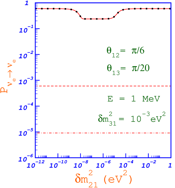
Figure 1: Several components of the electron neutrino survival probability given in Eq. (29). In this figure $\theta_{13}=\pi/6$, $\theta_{13}=\pi/20$, $E_{\nu}=1$ MeV, and $\delta m_{31}^{2}=10^{-3}$ eV². The upper solid line is the total survival probability. The filled squares on top of the figure represent the contribution of the term proportional to $\cos^{4}{\theta_{13}}$ alone to the survival probability. The middle long-dashed line is the contribution of the term proportional to $\sin^{4}{\theta_{13}}$ alone to the survival probability. The lower dash-dotted line is the contribution of the correction terms proportional to $\xi$ only.

For $\xi=0$ Eq. (29) reduces to the formula widely used in the literature (see e.g. Refs. Fogli:2000bk ; Kuo:1989qe ). We show the relative contributions of various terms to the survival probability given in Eq. (29) in Fig. 1. We picked values of the neutrino parameters representative of the solar neutrino results in this figure. The upper solid line is the total survival probability numerically calculated for the 3-flavor mixing by solving the neutrino evolution equation, Eq. (3), exactly using the method of Ref. Ohlsson:1999um . The filled squares on top of the figure represent the contribution of the term proportional to $\cos^{4}{\theta_{13}}$ alone (the first term in the right side of Eq. (29)) to the survival probability in the approximation described above. One observes that this term alone is an excellent approximation to the total probability. To illustrate this we plot separately the contribution of the term proportional to $\sin^{4}{\theta_{13}}$ alone to the survival probability (the long-dashed line in the middle). Clearly the second term is approximately three orders of magnitude smaller than the first one. The correction terms proportional to the parameter $\xi$ are even smaller by two more orders of magnitude indicating the validity of our expansion in terms of the parameter $\xi$. It is worth emphasizing that the quantity $\delta m_{31}^{2}$ enters the survival probability in Eq. (29) only through the terms proportional to $\xi$, hence its effect is minimal: For solar neutrinos the 3-flavor survival probability depends only on two mixing angles, $\theta_{12}$, $\theta_{13}$, and one mass-difference squared, $\delta m_{21}^{2}$. Having gained confidence in the validity of Eq. (29), we use it in our analysis.

III Statistical Analysis

There is an extensive literature describing methods to calculate the goodness of a fit and confidence levels of allowed regions (See e.g. Refs. Feldman:1997qc ; Fogli:2002pt ; Garzelli:2000yf ; Gonzalez-Garcia:2002dz and other references we cite below). In our global analysis, we use the “covariance approach”, in which least-squares function for solar data is defined as

$$\chi^{\,2}_{\,\odot}=\sum_{ij}\,(R_{\,i}^{\,exp}-R_{\,i}^{\,th})\,\sigma^{-2}_{\,ij}\,(R_{\,j}^{\,exp}-R_{\,j}^{\,th})\,,$$ (30)

where $R_{\,i}^{\,exp}$ and $R_{\,i}^{\,th}$ are the experimental values and theoretical predictions of the observables respectively and $\sigma^{\,-2}$ is the inverse of the covariance error matrix built from the statistical and systematic errors considering mutual correlations.

We use 80 data points in our analysis; the total rate of the chlorine experiment (Homestake), the average rate of the gallium experiments (SAGE, GALLEX, GNO), 44 data points from the SK zenith-angle-spectrum and 34 data points from the SNO day-night-spectrum. The only correlation between the rates of the water Cerenkov experiments and radiochemical experiments is the uncertainty in the ${}^{8}B$ flux. Since we fit the shape of the spectrum for water Cerenkov experiments in our analysis, the covariance error matrix can be block diagonalized. We write contributions to $\chi^{2}_{\,\odot}$ from the rates of the radiochemical experiments, the SK zenith-angle-spectrum, and the SNO day-night-spectrum explicitly:

$$\chi^{\,2}_{\,\odot}=\chi^{\,2}_{\,{\rm Cl,Ga\,Rates}}+\chi^{\,2}_{\rm\,SK}+\chi^{\,2}_{\rm\,SNO}.$$ (31)

SK and SNO uses the pattern and intensity of the Cerenkov light generated by the recoiling electron in order to detect events due to electron scattering (ES):

$$\nu_{x}+e^{-} \to \nu_{x}+e^{-}\ \text{ (ES)}.$$ (32)

ES is sensitive to all neutrino flavors with reduced sensitivity to non-electron-neutrino components. Since SNO contains heavy water it is sensitive to charge-current (CC) and neutral-current (NC) reactions in addition to ES:

$$\nu_{e}+d \to p+p+e^{-}\ ,\text{ (CC)},$$ (33)

$$\nu_{x}+d \to n+p+\nu_{x}\ ,\text{ (NC).}$$ (34)

The Cerenkov light generated by the recoiling electron is used to observe the CC events while the gamma ray from the neutron capture on deuterium is used to detect NC events. Time, location, direction, and energy of the CC events allow reconstruction of the solar neutrino spectrum.

Since Cerenkov experiments have a higher threshold energy they are sensitive to only ${}^{8}B$ and $hep$ neutrinos. The $hep$ neutrino flux is much smaller than the ${}^{8}B$ neutrino flux, but $hep$ neutrinos are somewhat more energetic. The production regions for these two components of the neutrino flux are not much different. For the sake of simplicity instead of dealing with two different sources of neutrinos, we add $hep$ neutrino spectrum to the ${}^{8}B$ neutrino spectrum

$$\lambda_{B}(E_{\nu}) \rightarrow \frac{\phi_{B}\lambda_{B}(E_{\nu})+\phi_{hep}\lambda_{hep}(E_{\nu})}{\phi_{B}+\phi_{hep}},$$ (35)

$$\phi_{B} \rightarrow \phi_{B}+\phi_{hep},$$ (36)

and use them as a single source in the analysis of Cerenkov experiments.

Cerenkov experiments are also live-time experiments. They can measure separate day and night rates or even divide their night rate into several zenith angle “$\alpha$” bins. We may expect to see a different rate for each of these bins since MSW mechanism predicts earth regeneration effects at night when neutrinos pass through several layers of Earth material. We incorporate those effects into our analysis by calculating the survival probability numerically at each zenith angle using a step function density approximation to the Preliminary Earth Model Dziewonski:xy . Survival probability for each zenith-angle bin is calculated by averaging the probability weighted with the exposure function “$f(\alpha)$” of the detector. For SK we used exposure function given in Ref. Bahcall:1997jc . For SNO we only used day-night bins and live-time information from Ref. HOWTOSNO . For any zenith bin between $\alpha_{min}^{j}$ and $\alpha_{max}^{j}$, the “weighted” average survival probability $\langle P^{\,j}(\nu_{e}\rightarrow\nu_{e},E_{\nu})\rangle$ is:

$$\langle P^{\,j}(\nu_{e}\rightarrow\nu_{e},E_{\nu})\rangle=\frac{\int_{\alpha_{min}^{j}}^{\alpha_{max}^{j}}f(\alpha)P^{\,}(\nu_{e}\rightarrow\nu_{e},E_{\nu},\alpha)\,d\alpha}{\int_{\alpha_{min}^{j}}^{\alpha_{max}^{j}}f(\alpha)\,d\alpha}$$ (37)

SK measures the kinetic energy of the recoiling electron and reports the data divided into several kinetic energy intervals. The kinetic energy assigned to the event by the detector is not always same as the true kinetic energy, instead it has a distribution around actual kinetic energy. This is characterized by a Gaussian shaped response function Bahcall:1996ha :

$$R(T,\,T^{\prime}) = \frac{1}{\sqrt{2\pi}s_{\rm SK}}\exp\left[{-\frac{(T-T^{\prime})^{2}}{2s_{\rm SK}^{2}}}\right]\ ,$$ (38)

$$s_{\rm SK} = 0.47\sqrt{T^{\prime}}\>\text{MeV},$$ (39)

where $s_{\rm SK}$ is the width of the Gaussian Faid:1996nx , $T^{\prime}$ is the actual kinetic energy of the recoiling electron and $T$ is the kinetic energy assigned to the same event by the detector (in Eqs. (38) and (39) both $T$ and $T^{\prime}$ are in MeV). By convolving differential ES cross sections of Ref. Bahcall:1995mm with energy response function of the detector at each kinetic energy interval $i$, we get the “corrected” cross sections corresponding to the kinetic energy bin $i$:

$$\sigma_{\nu_{e},\nu_{x}}^{i}(E_{\nu})=\int_{T_{min}^{i}}^{T_{max}^{i}}\!dT\int_{0}^{T_{max}^{\prime}}\!dT^{\prime}\,R(T,\,T^{\prime})\,\frac{d\sigma_{\nu_{e},\nu_{x}}(E_{\nu},\,T^{\prime})}{dT^{\prime}}\ ,$$ (40)

where $T_{max}^{\prime}=E_{\nu}/(1+m_{e}/2E_{\nu})$ is the maximum kinetic energy that any electron can have due to kinematical limits. After this step we have all the ingredients to calculate the rates for the zenith-spectrum bins, weighted survival probabilities for zenith-angle bins ($\langle P^{\,j}(\nu_{e}\rightarrow\nu_{e},E_{\nu})\rangle$), and the corrected cross sections for kinetic energy spectrum bins ($\sigma_{\nu_{e},\nu_{x}}^{i}(E_{\nu})$). If we consider only oscillations into active flavors the theoretical rate at SK for each zenith-spectrum bin is

$$R^{SK}_{k}=R^{SK}_{i,j} = \phi_{B}\int\!dE_{\nu}\,\lambda_{B}(E_{\nu})[\sigma_{\nu_{e}}^{i}(E_{\nu})\langle P^{j}(\nu_{e}\rightarrow\nu_{e},E_{\nu},t)\rangle$$ (41)

$$+ \sigma_{\nu_{x}}^{i}(E_{\nu})(1-\langle P^{j}(\nu_{e}\rightarrow\nu_{e},E_{\nu},t)\rangle)],$$

where we use “$k$” as a collective index for zenith-spectrum bins instead of the pair “$i,j$”. SK reports the ratio of number of observed events to the number of expected events under no oscillation condition. Dividing the above rate with SSM expected value (i.e. with the survival probability is 1) we obtain ratios to be compared with those given in Ref. Fukuda:2002pe .

To calculate the error matrix for SK zenith-spectrum bins, experimental rates and uncertainties are taken from Fukuda:2002pe . For each zenith and energy bin SK reports rates and statistical and systematic uncertainties. We take the ${}^{8}B$ shape, energy scale and energy resolution uncertainties from Fogli:2002pt which are actually calculated under no-oscillation condition and may result in discrepancies at higher confidence levels. An additional overall systematic offset error of 2.75% is added to all bins. In calculating $\chi^{\,2}_{\rm\,SK}$ we introduce a free normalization parameter “$\eta$” and minimize $\chi^{\,2}_{\rm\,SK}$ with respect to $\eta$. In this way the total ${}^{8}B$ flux allowed to float freely.

$$\chi^{\,2}_{\rm\,SK}=\sum_{ij}\,(R_{\,i}^{\,exp}-\eta R_{\,i}^{\,th})\,\sigma^{-2}_{\,ij}\,(R_{\,j}^{\,exp}-\eta R_{\,j}^{\,th})\,,$$ (42)

SNO response function for electrons is Ahmad:2002jz :

$$R(T,\,T^{\prime}) = \frac{1}{\sqrt{2\pi}s_{\rm SNO}}\exp\left[{-\frac{(T-T^{\prime})^{2}}{2s_{\rm SNO}^{2}}}\right]\ ,$$ (43)

$$s_{\rm SNO} = (-0.0684+0.331\sqrt{T^{\prime}}+0.0425T^{\prime})\text{ MeV},$$ (44)

“Corrected” ES and CC cross sections can be obtained in a similar fashion as we did for SK (cf. Eq. ( 40)). NC events are mono-energetic. Neutrons are first thermalized and then captured on deuterium. All NC events originally have same energy, $T_{NC}=5.08$ MeV. Their response function is HOWTOSNO

$$R(T) = \frac{1}{\sqrt{2\pi}s_{\rm NC}}\exp\left[{-\frac{(T-T_{NC})^{2}}{2s^{2}_{\rm NC}}}\right]\ ,$$ (45)

$$s_{\rm NC} = 1.11\text{MeV},$$ (46)

and the corresponding “corrected” cross sections are:

$$\sigma_{NC}^{i}(E_{\nu})=\int_{T_{min}^{i}}^{T_{max}^{i}}\!dTR(T)\,\frac{d\sigma_{NC}(E_{\nu},\,T)}{dT}\ .$$ (47)

The response function of Eq. (45) spreads the neutral current events in energy. We use the “forward-fitting” technique described in HOWTOSNO to calculate $\chi^{\,2}_{\,SNO}$. Event rates for each type of reaction are

$$R^{ES}_{k}=R^{ES}_{i,j} = \phi_{B}\int\!dE_{\nu}\,\lambda_{B}(E_{\nu})\big{[}\sigma_{\nu_{e}}^{i}(E_{\nu})\langle P_{ee}^{j}(E_{\nu},t)\rangle+\sigma_{\nu_{x}}^{i}(E_{\nu})(1-\langle P_{ee}^{j}(E_{\nu},t)\rangle)\big{]},$$ (48)

$$R^{CC}_{k}=R^{CC}_{i,j} = \phi_{B}\int\!dE_{\nu}\,\lambda_{B}(E_{\nu})\big{[}\sigma_{CC}^{i}(E_{\nu})\langle P_{ee}^{j}(E_{\nu},t)\rangle\big{]},$$ (49)

$$R^{NC}_{k}=R^{NC}_{i,j} = \phi_{B}\int\!dE_{\nu}\,\lambda_{B}(E_{\nu})\big{[}\sigma_{NC}^{i}(E_{\nu})\big{]}.$$ (50)

In our calculations we used the neutrino-deuteron cross-sections of Ref. Butler:1999sv calculated using the effective field theory approach. We fixed the counter-term, $L_{1A}$, of this approach so that it reproduces the calculation of Ref. Ying:1991tf which incorporates the first-forbidden matrix elements in the calculation of the neutrino-deuteron cross sections. Theoretically expected rate is calculated by adding background contributions like the so-called Low Energy Background (LB) and Neutron Background (NB) to the sum of CC, NC and ES events. We take these background contributions from Ref. HOWTOSNO . The expected event rate for each bin is

$$R^{th}_{k}=R^{ES}_{k}+R^{CC}_{k}+R^{NC}_{k}+R^{LB}_{k}+R^{NB}_{k}$$ (51)

In calculating error matrix for SNO zenith-spectrum bins, experimental rates and uncertainties are taken from Ref. HOWTOSNO . Statistical errors are calculated from the data reported by SNO and systematic uncertainties (shape scale and resolution) are taken from Ref. Fogli:2002pt . Other systematics like vertex accuracy, neutron-capture efficiency, etc. are taken from Ref. Ahmad:2002jz . In calculating $\chi^{\,2}_{\rm\,SNO}$ we multiply sum of CC, NC and ES events (without backgrounds) by a free normalization parameter “$\eta$” and minimize $\chi^{\,2}_{\rm\,SNO}$ with respect to $\eta$ as we did for SK (cf. Eq. (42). In this manner total ${}^{8}B$ flux allowed to float freely without affecting backgrounds.

The last component of $\chi^{\,2}_{\,\odot}$ is from the radiochemical experiments. In the evaluation of error matrix for $\chi^{\,2}_{\rm\,Cl,Ga\>Rates}$ we follow the procedure described in Ref. Fogli:1999zg .

In the presence of oscillations, energy averaged cross section $C^{th}_{mi}$ of neutrinos from source $m$ at detector $i$ can be calculated by convolving the neutrino spectrum $\lambda_{m}(E_{\nu})$ for the corresponding source, the cross section $\sigma_{i}(E_{\nu})$ for the corresponding detector and the survival probability $\langle P(\nu_{e}\rightarrow\nu_{e},E_{\nu})\rangle$ (averaged over source distributions in the Sun and weighted with the exposure function of each detector)

$$C^{th}_{mi}=\int\!dE_{\nu}\,\lambda_{m}(E_{\nu})\,\sigma_{i}(E_{\nu})\,\langle P(\nu_{e}\rightarrow\nu_{e},E_{\nu})\rangle.$$ (52)

Then event rate at detector $i$ is simply:

$$R^{th}_{i}=\sum_{m}R^{th}_{mi}=\sum_{m}\phi_{m}C^{th}_{mi}$$ (53)

SSM neutrino fluxes $\phi_{m}$ depend on the SSM input parameters $X_{k}$. The correlations between neutrino fluxes are parameterized by the logarithmic derivative:

$$\alpha_{\,ik}=\frac{\partial\ln\phi_{\,i}^{\,SSM}}{\partial\ln X_{\,k}}$$ (54)

$\Delta\ln X_{\,k}$ and $\Delta\ln C_{\,ki}$ are $1\sigma$ relative errors of SSM input parameters and energy averaged cross sections respectively. We adopt the values of these parameters from Ref. Fogli:1999zg .

From all above, one can write

$$\sigma^{\,2}_{\,ij}=\delta_{\,ij}\,\sigma_{\,i}^{\,exp}\sigma_{\,j}^{\,exp}+\delta_{\,ij}\sum_{k}R^{\,thr}_{\,ki}R^{\,thr}_{\,kj}\,(\Delta\ln C_{\,ki})^{\,2}+\sum_{mn}R_{\,mi}^{\,thr}\,R_{\,nj}^{\,thr}\sum_{k}\alpha_{\,mk}\,\alpha_{\,nk}\,(\Delta\ln X_{\,k})^{\,2}\ .$$ (55)

For global analysis we take:

$$\chi^{2}_{\rm Global}=\chi^{2}_{\,\odot}+\chi^{2}_{\rm KamLAND}$$ (56)

KamLAND detects reactor neutrinos in 1 kiloton of liquid scintillator through the reaction:

$$p+\overline{\nu}_{e}\rightarrow n+e^{+}.$$ (57)

We use the phenomenological parameterization of the energy spectrum of the incoming antineutrinos given in Ref. Vogel:iv :

$$\frac{{\rm d}N_{\bar{\nu}_{e}}}{{\rm d}E_{\nu}}\propto e^{a_{0}+a_{1}E_{\nu}+a_{2}E^{2}_{\nu}},$$ (58)

where the parameters vary with different isotopes. The spectra of antineutrinos coming from each detector, $\phi_{i}(t,E_{\nu})$, can be calculated using the thermal power and the isotropic composition of each detector. The effects of incomplete knowledge of the fuel composition are explored in Ref. Murayama:2000iq . We use the time-averaged fuel composition for the nuclear reactors given by the KamLAND collaboration :2002dm .

Survival probability for electron antineutrinos coming from the reactor $i$ is:

$$P({\overline{\nu}}_{e}\rightarrow{\overline{\nu}}_{e}) = \sin^{4}\theta_{13}+\cos^{4}\theta_{13}\left[1-\sum_{i}\sin^{2}2\theta_{12}\sin^{2}\left(\frac{1.27\Delta m^{2}_{21}L_{i}}{E_{\nu}}\right)\right],$$ (59)

where $L_{i}$ are the reactor-detector distances. We denote the energy resolution function of KamLAND by $R(T_{,}T^{\prime})$ where $T,T^{\prime}$ are the observed and the true positron energies. The energy resolution is given as $7.5\%/\sqrt{E({\rm MeV})}$ :2002dm . The number of expected events for each bin at KamLAND can be calculated by convolving the cross section, $\sigma(E_{\nu})$, with the reactor spectra, survival probabilities and the resolution function of KamLAND:

$$N_{i}^{\rm th}=\int dE_{\nu}\sigma(E_{\nu})\sum_{j}\frac{\phi_{j}(t,E_{\nu})}{L_{j}^{2}}P_{j}({\overline{\nu}}_{e}\rightarrow{\overline{\nu}}_{e},E_{\nu})\int dTR(T,T^{\prime})\,,$$ (60)

where the electron kinetic energy is $T^{\prime}\sim E_{\nu}-0.8$ MeV, and $\sigma(E_{\nu})$ is the lowest order cross section given in Refs. Vogel:1983hi ; Vogel:1999zy :

$$\sigma(E_{\nu})=\frac{2\pi^{2}}{m_{e}^{5}f\tau_{n}}p_{e}E_{e}$$ (61)

in which $E_{e}=T^{\prime}+m_{e}$, $f=1.69$ is the integrated Fermi function for neutron beta decay, and $\tau_{n}$ is the neutron lifetime.

KamLAND reports its results in 13 bins above the threshold. Due to low statistics, we use the prescription of Hagiwara:fs in analyzing KamLAND data. We write

$$\chi^{2}_{\,KamLAND-Spect}=2\sum_{i}\left[(\eta N_{i}^{\,th}-N_{i}^{\,exp})+N_{i}^{\,exp}\ln\left(\frac{N_{i}^{\,exp}}{\eta N_{i}^{\,th}}\right)\right]+\frac{(\eta-1)^{2}}{\sigma_{\,sys}^{2}},$$ (62)

where $\sigma_{\,sys}^{2}=6.75\%$ is the systematic uncertainty, and minimize the sum in Eq. (62) with respect to $\eta$. For the total rate analysis we use

$$\chi^{2}_{\,KamLAND-Rate}=\frac{(N^{\,th}-N^{\,exp})^{2}}{\sigma_{\rm R}^{2}}\;,$$ (63)

with errors added in the quadrature to calculate $\sigma_{\rm R}^{2}$. $N^{\,exp}$ is given in :2002dm and $N^{\,th}$ is calculated at each value of oscillation parameters similar to the binned expected event rates.

IV Results and Conclusions

In our calculations we use the neutrino spectra given by the Standard Solar Model of Bahcall and collaborators Bahcall:2000nu . It it is numerically more convenient to follow the evolution of the matter eigenstates in the Sun and in the Earth (or mass eigenstates in vacuum), a procedure which we adopted. We take into account the distribution of various neutrino sources in the core of the Sun and resulting non-linear paths of the neutrinos. Thus neutrinos coming from the other side of the Sun may have double resonances. In the Sun we used the Landau-Zener approximation Balantekin:1996ag ; Haxton:dm ; Parke:1986jy . We divided the Sun into several shells which were in turn divided into several angular bins, calculated the derivative of the electron density in the Landau-Zener approximation numerically for both radial and non-radial neutrino paths and averaged the survival probabilities over the initial source distributions.

Survival probabilities in the Earth depend on zenith angles. As was described in the previous Section we adopted the Preliminary Earth Model density Dziewonski:xy to solve neutrino evolution oscillations numerically in the Earth.

In our calculations we ignore the possibility of density fluctuations in the Sun Loreti:1994ry ; Balantekin:1996pp . Recent data indicate that such fluctuations are less than one percent of the Standard Solar Model density Balantekin:2001dx . We similarly ignore possible mixing of sterile components. Sterile neutrinos can play a very important role in supernova r-process McLaughlin:1999pd ; Caldwell:1999zk ; Fetter:2002xx or the big-bang nucleosynthesis Abazajian:2001vt . It is worth emphasizing that active-sterile mixing can be too small to be detectable in solar neutrino experiments (for a discussion of various possibilities see e.g. Ref. Bahcall:2002zh ) and yet may still have significant astrophysical impact.

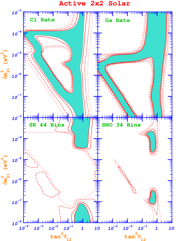
Figure 2: Allowed regions of the neutrino parameter space when each solar neutrino experiment is considered separately. In this figure $\theta_{13}$ is taken to be zero. The shaded areas are the 90 % confidence level regions. 95 % (solid line), 99 % (log-dashed line), and 99.73 % (dotted-line) confidence levels are also shown.

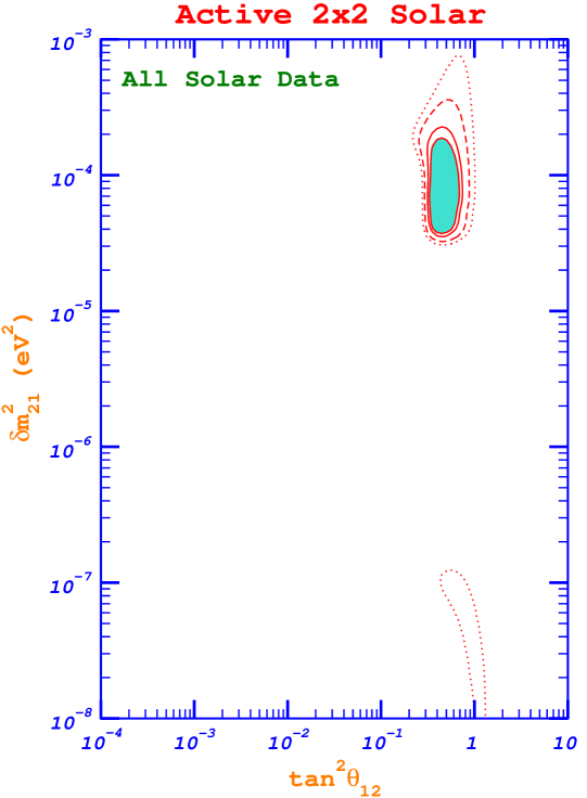
Figure 3: Allowed regions of the neutrino parameter space when all solar neutrino experiments (chlorine, all three gallium, SNO and SK experiments) are included in the analysis. In this figure $\theta_{13}$ is taken to be zero. The shaded area is the 90 % confidence level region. 95 % (solid line), 99 % (log-dashed line), and 99.73 % (dotted-line) confidence levels are also shown.

We first present calculations where we took the value of $\theta_{13}$ to be zero and considered only the solar neutrino data. Allowed regions of neutrino parameter space when each solar neutrino experiment is considered separately are shown in Fig. 2. One observes that either Sudbury Neutrino Observatory or SuperKamiokande individually already significantly limit the neutrino parameter space. Our results agree well with the own analyses of these experimental groups. Allowed regions of neutrino parameter space when all solar neutrino experiments are combined together are shown in Fig. 3. The combined solar neutrino data already rule out the so-called LOW region where $\delta m_{12}^{2}<10^{-7}$ eV² at the 99 % confidence level. We find the best fit (minimum $\chi^{2}$) values of neutrino parameters to be $\tan^{2}\theta_{12}\sim 0.45$ and $\delta m_{12}^{2}\sim 7.08\times 10^{-5}$ eV² from our combined analysis of all the solar neutrino data. Our minimum $\chi^{2}$ value is 67.2 for 80 data points and 2 parameters.

We next turn our attention to KamLAND data while still keeping the value of $\theta_{13}$ to be zero. In the upper panels of Fig. 4 we display allowed regions of the neutrino parameter space from the KamLAND data only. (Results with using the total rate only is at the left-hand side and results with using the binned data, which provide more information about the neutrino spectrum, is at the right-hand side). The result of our global analysis combining the solar date with data from KamLAND is shown at the lower right-hand side panel. For convenience of presentation we do not show the lower values of $\delta m_{12}^{2}$ on the graph, but the LOW solution is completely eliminated. For comparison we re-plot the neutrino parameter space obtained from the solar neutrino data only at the lower left-hand side of the Figure. KamLAND data significantly shrinks the LMA region (the lower right-hand side of the Figure). We find the best fit (minimum $\chi^{2}$) values of neutrino parameters to be $\tan^{2}\theta_{12}\sim 0.46$ and $\delta m_{12}^{2}\sim 7.1\times 10^{-5}$ eV² from our combined analysis of all the solar neutrino and KamLAND data. Our minimum $\chi^{2}$ value is 73.2 for $\rm{80+13}$ data points and 2 parameters. Inclusion of the KamLAND data does not noticeably change the best fit values of the neutrino parameters, however KamLAND, being a terrestrial experiment with very different statistical errors, provides a completely independent test of the results from the solar neutrino experiments. Fig. 4 also illustrates that mixing of the (solar) neutrinos and (reactor) antineutrinos are very similar, very likely to be identical.

It is instructive to investigate how well the neutrino parameter space is constrained. To this extend we plot allowed regions of the neutrino parameter spaces obtained by combining data from a single solar neutrino experiment with the KamLAND data in Fig. 5. In calculating the parameter space shown in this Figure we continued to take the value of $\theta_{13}$ to be zero. We observe that any single solar neutrino experiment taken together with KamLAND significantly constraints the parameter space. The LOW region, which is not shown on these plots, is again completely eliminated for each case. Real-time Cerenkov detectors are slightly more constraining than the radiochemical experiments in this regard. It is also interesting to realize that one no longer needs all the solar neutrino experiments to determine the neutrino parameters. We are getting closer to realizing the initial goal of the solar neutrino experiments, eloquently stated in the seminal papers of Bahcall and Davis bahcalldavis , namely to use solar neutrino data to better understand the Sun. (For a preliminary effort see Ref. Balantekin:1997fr ).

We next examine the effects of a non-zero value of $\theta_{13}$. In Fig. 6 we show how the parameter space changes as a function of $\theta_{13}$ when $\theta_{12}$ is kept fixed. Here we use Eq. (29) to calculate the 3-flavor neutrino survival probability and perform the $\chi^{2}$ analysis for three parameters ($\theta_{12}$, $\theta_{13}$, and $\delta m_{12}^{2}$). We find the best fit (minimum $\chi^{2}$) values of neutrino parameters to be $\tan^{2}\theta_{12}\sim 0.46$, $\cos^{4}\theta_{13}\sim 1$, and $\delta m_{12}^{2}\sim 7.1\times 10^{-5}$ eV². Note that the confidence level regions in the pair that corresponds to the best fit (the lowest right-hand side pair in Fig. 6) are larger than the corresponding pair obtained with 2-flavor analysis (lower pair in Fig. 4) since as one goes from the former to the latter the number of parameters are reduced by one. To illustrate the change in the quality of the fit as $\tan^{2}\theta_{12}$ is changed we present confidence levels for a several values of $\tan^{2}\theta_{12}$, some of which are clearly very far away from the optimal solution. It is interesting to note that the combined Solar neutrino and KamLAND date provide a limit of $\cos^{4}\theta_{13}>0.8$ at the 90 % confidence level. We are able to put such a limit since we investigated confidence levels for larger values of $\theta_{13}$, otherwise solar data alone are not sufficient to constraint this angle (cf. Ref Fogli:2002pb ). This limit currently is not as good as the one obtained from the completed reactor disappearance experiments Apollonio:1999ae ; Boehm:2001ik ; however the situation may change after a few years of data taking at KamLAND Gonzalez-Garcia:2001zy .

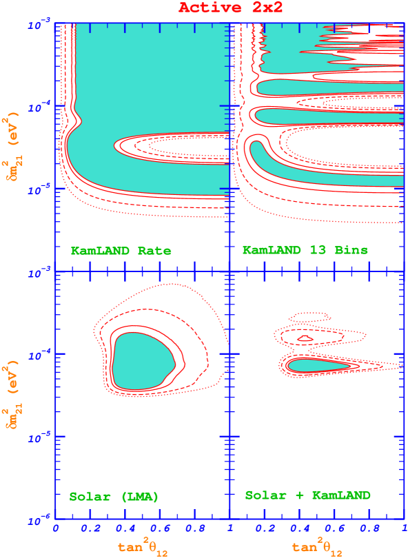
Figure 4: Allowed regions of the neutrino parameter space with $\theta_{13}$ taken to be zero. In the upper-left panel only KamLAND total rate and in the upper-right-hand panel binned KamLAND data are used. Lower-left hand panel depicts the LMA solution obtained from only the solar neutrino experiments. All solar neutrino experiments are combined with the KamLAND date to obtain the lower right-hand panel. The shaded areas are the 90 % confidence level regions. 95 % (solid line), 99 % (log-dashed line), and 99.73 % (dotted-line) confidence levels are also shown.

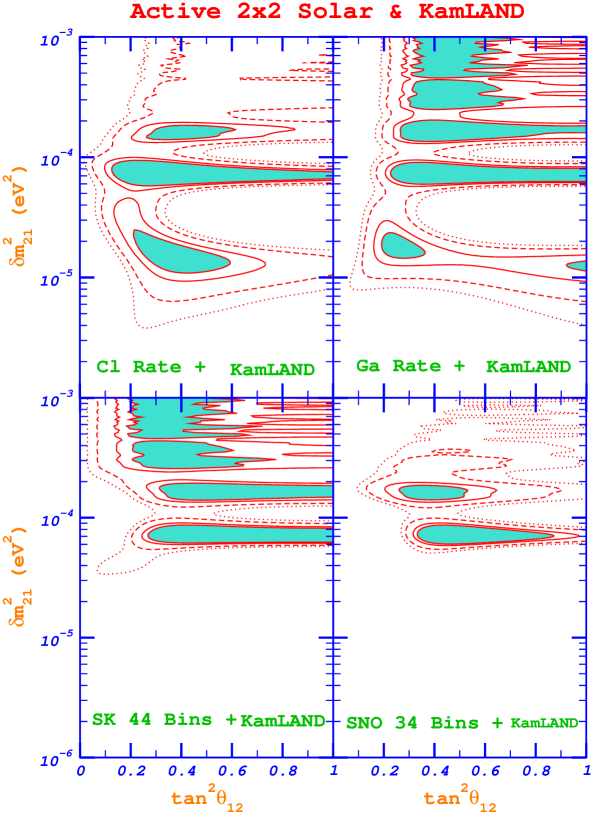
Figure 5: Allowed regions of the neutrino parameter space obtained when data from a single solar neutrino experiment is combined with the KamLAND data. The shaded areas are the 90 % confidence level regions. 95 % (solid line), 99 % (log-dashed line), and 99.73 % (dotted-line) confidence levels are also shown.

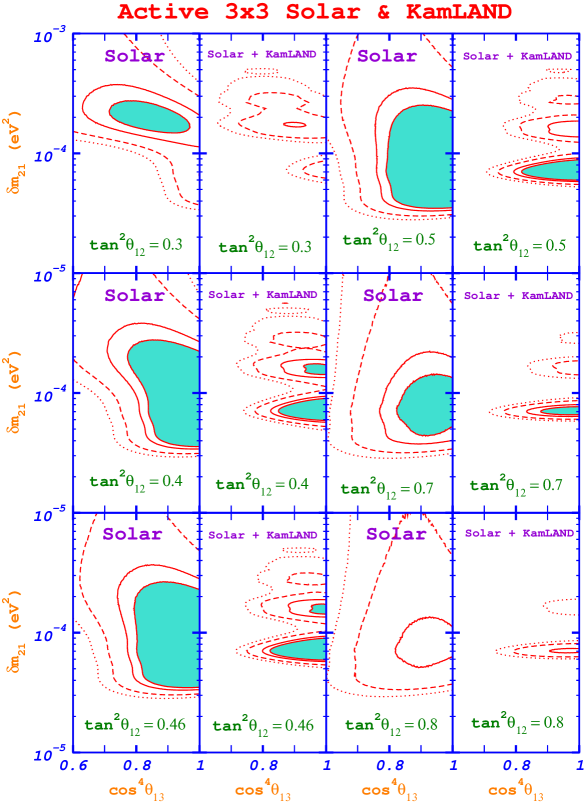
Figure 6: Allowed regions of neutrino parameter space when both mixing angles $\theta_{12}$ and $\theta_{13}$ are varied. Six pairs of $\delta m_{21}^{2}$ vs. $\cos^{4}\theta_{13}$ plots are presented for representative values of $\tan^{2}\theta_{12}$ (0.3, 0.4, 0.43, 0.46, 0.5, 0.7, and 0.8). The figures on the left-hand side of each pair are obtained from the combination of all solar neutrino experiments while the figures on the right-hand side of each pair also include the KamLAND data. The shaded areas are the 90 % confidence level regions. 95 % (solid line), 99 % (log-dashed line), and 99.73 % (dotted-line) confidence levels are also shown.

References

- (1) Q. R. Ahmad et al. [SNO Collaboration], Phys. Rev. Lett. 87, 071301 (2001) [arXiv:nucl-ex/0106015].
- (2) S. Fukuda et al. [Super-Kamiokande Collaboration], Phys. Rev. Lett. 86, 5651 (2001) [arXiv:hep-ex/0103032], S. Fukuda et al. [Super-Kamiokande Collaboration], Phys. Rev. Lett. 86, 5656 (2001) [arXiv:hep-ex/0103033].
- (3) Q. R. Ahmad et al. [SNO Collaboration], Phys. Rev. Lett. 89, 011301 (2002) [arXiv:nucl-ex/0204008].
- (4) Q. R. Ahmad et al. [SNO Collaboration], Phys. Rev. Lett. 89, 011302 (2002) [arXiv:nucl-ex/0204009].
- (5) J. N. Bahcall, M. H. Pinsonneault and S. Basu, Astrophys. J. 555, 990 (2001) [arXiv:astro-ph/0010346].
- (6) B. T. Cleveland et al., Astrophys. J. 496, 505 (1998).
- (7) J. N. Abdurashitov et al. [SAGE Collaboration], J. Exp. Theor. Phys. 95, 181 (2002) [Zh. Eksp. Teor. Fiz. 122, 211 (2002)] [arXiv:astro-ph/0204245].
- (8) W. Hampel et al. [GALLEX Collaboration], Phys. Lett. B 447, 127 (1999).
- (9) M. Altmann et al. [GNO Collaboration], Phys. Lett. B 490, 16 (2000) [arXiv:hep-ex/0006034].
- (10) See e.g. J. N. Bahcall, M. C. Gonzalez-Garcia and C. Pena-Garay, JHEP 0207, 054 (2002) [arXiv:hep-ph/0204314].
- (11) K. Eguchi et al. [KamLAND Collaboration], arXiv:hep-ex/0212021.
- (12) J. N. Bahcall, M. C. Gonzalez-Garcia and C. Pena-Garay, arXiv:hep-ph/0212147;
- (13) G. L. Fogli, E. Lisi, A. Marrone, D. Montanino, A. Palazzo and A. M. Rotunno, arXiv:hep-ph/0212127.
- (14) V. Barger and D. Marfatia, arXiv:hep-ph/0212126.
- (15) M. Maltoni, T. Schwetz and J. W. Valle, arXiv:hep-ph/0212129.
- (16) A. Bandyopadhyay, S. Choubey, R. Gandhi, S. Goswami and D. P. Roy, arXiv:hep-ph/0212146.
- (17) H. Nunokawa, W. J. Teves and R. Z. Funchal, arXiv:hep-ph/0212202.
- (18) P. Aliani, V. Antonelli, M. Picariello and E. Torrente-Lujan, arXiv:hep-ph/0212212.
- (19) P. C. de Holanda and A. Y. Smirnov, arXiv:hep-ph/0212270.
- (20) P. Creminelli, G. Signorelli and A. Strumia, JHEP 0105, 052 (2001) [arXiv:hep-ph/0102234].
- (21) D. Beavis et al., arXiv:hep-ex/0205040.
- (22) H. Minakata, H. Nunokawa and S. Parke, Phys. Rev. D 66, 093012 (2002) [arXiv:hep-ph/0208163].
- (23) E. K. Akhmedov, P. Huber, M. Lindner and T. Ohlsson, Nucl. Phys. B 608, 394 (2001) [arXiv:hep-ph/0105029].
- (24) L. Wolfenstein, Phys. Rev. D 17, 2369 (1978).
- (25) S. P. Mikheev and A. Y. Smirnov, Sov. J. Nucl. Phys. 42, 913 (1985) [Yad. Fiz. 42, 1441 (1985)].
- (26) S. P. Mikheev and A. Y. Smirnov, Nuovo Cim. C 9, 17 (1986).
- (27) A. B. Balantekin and G. M. Fuller, Phys. Lett. B 471, 195 (1999) [arXiv:hep-ph/9908465].
- (28) T. K. Kuo and J. Pantaleone, Phys. Rev. Lett. 57, 1805 (1986).
- (29) C. Bemporad, G. Gratta and P. Vogel, Rev. Mod. Phys. 74, 297 (2002) [arXiv:hep-ph/0107277].
- (30) M. Apollonio et al. [CHOOZ Collaboration], Phys. Lett. B 466, 415 (1999) [arXiv:hep-ex/9907037].
- (31) F. Boehm et al., Phys. Rev. D 64, 112001 (2001) [arXiv:hep-ex/0107009].
- (32) S. Fukuda et al. [Super-Kamiokande Collaboration], Phys. Rev. Lett. 85, 3999 (2000) [arXiv:hep-ex/0009001].
- (33) J. N. Bahcall, “Neutrino Astrophysics,” (Cambridge University Press, Cambridge, 1989).
- (34) A. B. Balantekin and N. Takigawa, Annals Phys. 160, 441 (1985).
- (35) G. L. Fogli, E. Lisi and D. Montanino, Phys. Rev. D 54, 2048 (1996) [arXiv:hep-ph/9605273].
- (36) G. L. Fogli, E. Lisi, D. Montanino and A. Palazzo, Phys. Rev. D 62, 113004 (2000) [arXiv:hep-ph/0005261].
- (37) A. B. Balantekin, Phys. Rept. 315, 123 (1999) [arXiv:hep-ph/9808281].
- (38) T. K. Kuo and J. Pantaleone, Rev. Mod. Phys. 61, 937 (1989).
- (39) S. T. Petcov, Phys. Lett. B 200, 373 (1988).
- (40) D. Notzold, Phys. Rev. D 36, 1625 (1987).
- (41) M. Bruggen, W. C. Haxton and Y. Z. Qian, Phys. Rev. D 51, 4028 (1995).
- (42) A. B. Balantekin, Phys. Rev. D 58, 013001 (1998) [arXiv:hep-ph/9712304].
- (43) H. Lehmann, P. Osland and T. T. Wu, Commun. Math. Phys. 219, 77 (2001) [arXiv:hep-ph/0006213].
- (44) A. B. Balantekin and J. F. Beacom, Phys. Rev. D 54, 6323 (1996) [arXiv:hep-ph/9606353]; A. B. Balantekin, S. H. Fricke and P. J. Hatchell, Phys. Rev. D 38, 935 (1988);
- (45) A. B. Balantekin, J. F. Beacom and J. M. Fetter, Phys. Lett. B 427, 317 (1998) [arXiv:hep-ph/9712390].
- (46) E. Lisi, A. Marrone, D. Montanino, A. Palazzo and S. T. Petcov, Phys. Rev. D 63, 093002 (2001) [arXiv:hep-ph/0011306].
- (47) T. Ohlsson and H. Snellman, Phys. Lett. B 474, 153 (2000) [arXiv:hep-ph/9912295]; T. Ohlsson and H. Snellman, J. Math. Phys. 41, 2768 (2000) [Erratum-ibid. 42, 2345 (2001)] [arXiv:hep-ph/9910546]; T. Ohlsson and H. Snellman, Eur. Phys. J. C 20, 507 (2001) [arXiv:hep-ph/0103252].
- (48) G. J. Feldman and R. D. Cousins, Phys. Rev. D 57, 3873 (1998) [arXiv:physics/9711021].
- (49) G. L. Fogli, E. Lisi, A. Marrone, D. Montanino and A. Palazzo, Phys. Rev. D 66, 053010 (2002) [arXiv:hep-ph/0206162].
- (50) M. V. Garzelli and C. Giunti, Astropart. Phys. 17, 205 (2002) [arXiv:hep-ph/0007155]; M. V. Garzelli and C. Giunti, Phys. Rev. D 65, 093005 (2002) [arXiv:hep-ph/0111254]; M. V. Garzelli and C. Giunti, JHEP 0112, 017 (2001) [arXiv:hep-ph/0108191].
- (51) M. C. Gonzalez-Garcia and Y. Nir, arXiv:hep-ph/0202058.
- (52) A. M. Dziewonski and D. L. Anderson, Phys. Earth Planet. Interiors 25, 297 (1981).
- (53) J. N. Bahcall and P. I. Krastev, Phys. Rev. C 56, 2839 (1997) [arXiv:hep-ph/9706239].
- (54) SNO Collaboration, Data Page, http://www.sno.phy.queensu.ca/sno/prlwebpage.
- (55) J. N. Bahcall, P. I. Krastev and E. Lisi, Phys. Rev. C 55, 494 (1997) [arXiv:nucl-ex/9610010].
- (56) B. Faid, G. L. Fogli, E. Lisi and D. Montanino, Phys. Rev. D 55, 1353 (1997) [arXiv:hep-ph/9608311].
- (57) J. N. Bahcall, M. Kamionkowski and A. Sirlin, Phys. Rev. D 51, 6146 (1995) [arXiv:astro-ph/9502003].
- (58) S. Fukuda et al. [Super-Kamiokande Collaboration], Phys. Lett. B 539, 179 (2002) [arXiv:hep-ex/0205075].
- (59) M. Butler and J. W. Chen, Nucl. Phys. A 675, 575 (2000) [arXiv:nucl-th/9905059]; M. Butler, J. W. Chen and X. Kong, Phys. Rev. C 63, 035501 (2001) [arXiv:nucl-th/0008032].
- (60) S. Ying, W. C. Haxton and E. M. Henley, Phys. Rev. C 45, 1982 (1992).
- (61) G. L. Fogli, E. Lisi, D. Montanino and A. Palazzo, Phys. Rev. D 62, 013002 (2000) [arXiv:hep-ph/9912231].
- (62) P. Vogel and J. Engel, Phys. Rev. D 39, 3378 (1989).
- (63) H. Murayama and A. Pierce, Phys. Rev. D 65, 013012 (2002) [arXiv:hep-ph/0012075].
- (64) P. Vogel, Phys. Rev. D 29, 1918 (1984).
- (65) P. Vogel and J. F. Beacom, Phys. Rev. D 60, 053003 (1999) [arXiv:hep-ph/9903554].
- (66) K. Hagiwara et al. [Particle Data Group Collaboration], Phys. Rev. D 66, 010001 (2002).
- (67) W. C. Haxton, Phys. Rev. Lett. 57, 1271 (1986).
- (68) S. J. Parke, Phys. Rev. Lett. 57, 1275 (1986).
- (69) F. N. Loreti and A. B. Balantekin, Phys. Rev. D 50, 4762 (1994) [arXiv:nucl-th/9406003].
- (70) A. B. Balantekin, J. M. Fetter and F. N. Loreti, Phys. Rev. D 54, 3941 (1996) [arXiv:astro-ph/9604061].
- (71) A. B. Balantekin, Proceedings of International Nuclear Physics Conference (INPC 2001): Nuclear Physics and the 21st Century, Berkeley, California, 30 Jul - 3 Aug 2001, E. Norman, L. Schroeder, and G. Wozniak, Eds. AIP Conference Proceedings, V. 610 [arXiv:hep-ph/0109163].
- (72) G. C. McLaughlin, J. M. Fetter, A. B. Balantekin and G. M. Fuller, Phys. Rev. C 59, 2873 (1999) [arXiv:astro-ph/9902106].
- (73) D. O. Caldwell, G. M. Fuller and Y. Z. Qian, Phys. Rev. D 61, 123005 (2000) [arXiv:astro-ph/9910175].
- (74) J. Fetter, G. C. McLaughlin, A. B. Balantekin and G. M. Fuller, arXiv:hep-ph/0205029.
- (75) K. Abazajian, G. M. Fuller and W. H. Tucker, Astrophys. J. 562, 593 (2001) [arXiv:astro-ph/0106002]; R. R. Volkas, Prog. Part. Nucl. Phys. 48, 161 (2002) [arXiv:hep-ph/0111326].
- (76) J. N. Bahcall, M. C. Gonzalez-Garcia and C. Pena-Garay, Phys. Rev. C 66, 035802 (2002) [arXiv:hep-ph/0204194]; V. D. Barger, B. Kayser, J. Learned, T. J. Weiler and K. Whisnant, Phys. Lett. B 489, 345 (2000) [arXiv:hep-ph/0008019].
- (77) J. N. Bahcall, Phys. Rev. Lett. 12, 300 (1964); R. Davis, Phys. Rev. Lett. 12, 303 (1964).
- (78) G. L. Fogli, G. Lettera, E. Lisi, A. Marrone, A. Palazzo and A. Rotunno, Phys. Rev. D 66, 093008 (2002) [arXiv:hep-ph/0208026].
- (79) M. C. Gonzalez-Garcia and C. Pena-Garay, Phys. Lett. B 527, 199 (2002) [arXiv:hep-ph/0111432]; V. D. Barger, D. Marfatia and B. P. Wood, Phys. Lett. B 498, 53 (2001) [arXiv:hep-ph/0011251].