All-Orders Singular Emission in Gauge Theories

Abstract

I present a class of functions unifying all singular limits for the emission of soft or collinear gluons in gauge-theory amplitudes at any order in perturbation theory. Each function is a generalization of the antenna functions of ref. SingleAntenna ; MultipleAntenna . The helicity-summed interferences these functions are thereby also generalizations to higher orders of the Catani–Seymour dipole factorization function.

I

Amplitudes in gauge theories have universal factorization and scaling behaviors as sets of massless momenta become collinear or soft. The study of these factorization properties goes back to the earliest quantum-mechanical studies of soft-photon emission by Bloch and Nordsieck BlochNordsieck . It has played an important role in our ability to make increasingly accurate predictions for scattering processes at high-energy colliders. An understanding of the factorization properties are necessary both to predictions at fixed order, and those relying on a summation of dominant logarithms.

Recent progress in two-loop calculations TwoloopSummary has opened the way for next-to-next-to-leading order (NNLO) calculations of jet production, both at lepton and hadron colliders. Completing this program, and obtaining numerical programs, will require further work on integrals over singular regions of gluon and quark-pair emission. These integrals will be rendered more tractable by a formalism which unifies the factorization behavior of amplitudes in the disparate collinear, soft, or mixed regions of phase space. Catani and Seymour proposed CataniSeymour such a formalism, the so-called dipole formalism, for one singular emission (one collinear pair or one soft gluon). I later wrote down SingleAntenna an equivalent formalism, at the level of the amplitude rather than the squared matrix element. This formalism generalizes MultipleAntenna to the emission of an arbitrary number of singular partons in tree-level amplitudes. The integrals over the factorization functions as further computed using a dimensional regulator in ref. CataniSeymour summarize in a universal fashion the infrared poles required to cancel those in one-loop virtual corrections.

Define an antenna function or amplitude via

$$\mathop{\rm Ant}\nolimits({\hat{a}},{\smash{{\hat{b}}}{}}\leftarrow a,1,\ldots,m,b)=\sum_{j=0}^{m}J(a,1,\ldots,j;{\hat{a}})J(j\!+\!1,\ldots,m,b;{\smash{{\hat{b}}}{}}),$$ (1)

where $J$ is a gluon (or quark) current as used in the Berends–Giele recurrence relations Recurrence . In the form given by Dixon DixonTASI , the gluon current (with opposite sign to Dixon’s) is,

$$J_{\mu}(1,\ldots,n)=$$

$$\hskip-42.67912pt-{id_{\mu\mu^{\prime}}(K_{1,n})\over K_{1,n}^{2}}\left[\sum_{j=1}^{n-1}V_{3}^{\mu^{\prime}\nu^{\prime}\rho^{\prime}}(K_{1,j},K_{j\!+\!1,n},-K_{1,n})d_{\nu\nu^{\prime}}(K_{1,j})d_{\rho\rho^{\prime}}(K_{j\!+\!1,n})J^{\nu}(1,\ldots,j)J^{\rho}(j\!+\!1,\ldots,n)\right.$$

$$\hskip-42.67912pt\hphantom{-{id_{\mu\mu^{\prime}}(K_{1,n})\over K_{1,n}^{2}}\Biggl{[}}\left.-\sum_{j_{1}=1}^{n-1}\sum_{j_{2}=j_{1}+1}^{n-1}V_{4}^{\mu^{\prime}\nu^{\prime}\rho^{\prime}\lambda^{\prime}}d_{\nu\nu^{\prime}}(K_{1,j_{1}})d_{\rho\rho^{\prime}}(K_{j_{1}\!+\!1,j_{2}})d_{\rho\rho^{\prime}}(K_{j_{2}\!+\!1,n})\right.$$

$$\hphantom{-{id_{\mu\mu^{\prime}}(K_{1,n})\over K_{1,n}^{2}}\Biggl{[}}\hphantom{\sum\sum\sum}\times\left.\vphantom{\sum_{j=1}^{1}}J^{\nu}(1,\ldots,j_{1})J^{\rho}(j_{1}\!+\!1,\ldots,j_{2})J^{\lambda}(j_{2}\!+\!1,\ldots,n)\right].$$

Here, $K_{i,j}=k_{i}+\cdots+k_{j}$; in eqn. (1), $J(1,\ldots,n;x)=\varepsilon_{x}\cdot J(1,\ldots,n)$ and the currents are to be evaluated in light-cone gauge, for which

$$V_{3}^{\mu\nu\rho}(P,Q,R)={i\over\sqrt{2}}\left[g^{\nu\rho}(P\!-\!Q)^{\mu}\!+\!g^{\rho\mu}(Q\!-\!R)^{\nu}\!+\!g^{\mu\nu}(R\!-\!P)^{\rho}\right];$$

$$V_{4}^{\mu\nu\rho\lambda}={i\over 2}\left[2g^{\mu\rho}g^{\nu\lambda}\!-\!g^{\mu\nu}g^{\rho\lambda}\!-\!g^{\mu\lambda}g^{\nu\rho}\right];\hskip 14.22636ptd_{\mu\nu}(k)=-g_{\mu\nu}+{q^{\mu}k^{\nu}\!+\!k^{\mu}q^{\nu}\over q\cdot k}.$$ (3)

The antenna amplitude describes in a unified way all leading singularities of tree amplitudes as the color-connected set of momenta $\{k_{a},k_{1},\ldots,k_{i}\}$ becomes collinear, likewise for $\{k_{j},\ldots,k_{n},k_{b}\}$, and as the momenta $\{k_{i\!+\!1},\ldots,k_{j\!-\!1}\}$ become soft,

$$A_{n}(\ldots,a,1,\ldots,m,b,\ldots)\buildrel k_{1},\ldots,k_{m}{\rm\ singular}\over{\relbar\mskip-0.5mu\joinrel\mskip-0.5mu\relbar\mskip-0.5mu\joinrel\longrightarrow}\mskip-8.0mu\sum_{{\rm ph.\ pol.}\ \lambda_{a,b}}\mathop{\rm Ant}\nolimits({\hat{a}}^{\lambda_{a}},{\smash{{\hat{b}}}{}}^{\lambda_{b}}\leftarrow a,1,\ldots,m,b)A_{n-m}(\ldots,-k_{{\hat{a}}}^{-\lambda_{a}},-k_{{\smash{{\hat{b}}}{}}}^{-\lambda_{b}},\ldots).$$

The momenta $k_{{\hat{a}},{\smash{{\hat{b}}}{}}}$ are reconstructed from the original momenta via reconstruction functions given in ref. MultipleAntenna .

In this Letter, I generalize the construction of ref. MultipleAntenna to higher orders in perturbation theory. To obtain such a generalization, we must first write down a formula for the higher-loop analog of the current $J$. (See ref. CataniGrazziniSoft for a related construction.) I will restrict attention here to leading-color amplitudes in the context of a color decomposition Color , so that only planar diagrams need be considered. These higher-loop analogs to the current will bear the same relation to higher-loop splitting amplitudes as do the tree-level currents to the tree-level multi-collinear splitting amplitudes: spinor products replace momentum fractions, adding phase and correlation information, and capturing a larger scope of singular behavior.

Higher-loop currents $J^{l\hbox{-\kern-0.14003pt}{}{\rm loop}}$ may be defined via their cuts,

$$\left.J^{l\hbox{-\kern-0.14003pt}{}{\rm loop}}(1^{\lambda_{1}},2^{\lambda_{2}},\ldots,m^{\lambda_{m}};P)\right|_{t_{c\cdots d}{\rm\ cut}}=$$

$$\hskip 14.22636pt\sum_{k=0}^{l-1}\,\sum_{j=2}^{l+1-k}\sum_{{\rm ph.\ pol.}\ \sigma_{i}}\int d{\rm LIPS}^{4-2\epsilon}(\ell_{1},\ldots,\ell_{j})\;J^{k\hbox{-\kern-0.14003pt}{}{\rm loop}}(1^{\lambda_{1}},\ldots,(c\!-\!1)^{\lambda_{c\!-\!1}},\ell_{1}^{-\sigma_{1}},\ldots,\ell_{j}^{-\sigma_{j}},(d\!+\!1)^{\lambda_{d\!+\!1}},\ldots,m;P)$$

$$\hskip 213.39566pt\times\,A_{d\!-\!c\!+\!j\!+\!1}^{(l\!+\!1\!-\!j\!-\!k)\hbox{-\kern-0.14003pt}{}{\rm loop}}(c^{\lambda_{c}},\ldots,d^{\lambda_{d}},-\ell_{j}^{\sigma_{j}},\ldots,-\ell_{1}^{\sigma_{1}}).$$ (4)

In this equation, $X^{0\hbox{-\kern-0.14003pt}{}{\rm loop}}$ means $X^{{\rm tree\vphantom{p}}}$. While the currents appearing here must be evaluated in light-cone gauge, the on-shell amplitudes on the other side of the cut may be evaluated in any gauge.

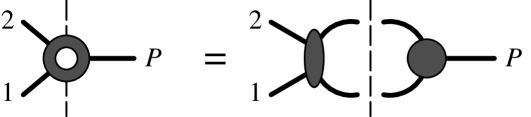
Figure 1: The one-loop three-point current is defined by its cut.

In the one-loop case, the three-point current has only one cut, illustrated in fig. 1, and we can reconstruct a loop integral from it,

$$J(1,2;P)= \mskip-25.0mu\sum_{{\rm ph.\ pol.}\ \sigma_{1},\sigma_{2}}\int{d^{4-2\epsilon}\ell\over(2\pi)^{4-2\epsilon}}\;{i\over\ell^{2}}J^{{\rm tree\vphantom{p}}}((\ell\!+\!a\!+\!b)^{-\sigma_{2}},-\ell^{-\sigma_{1}};P){i\over(\ell\!+\!k_{a}\!+\!k_{b})^{2}}A_{4}^{\rm tree\vphantom{p}}((-\ell\!-\!a\!-\!b)^{\sigma_{2}},1,2,\ell^{\sigma_{1}}).$$ (5)

The restriction to physical polarizations is important, as it will give rise to projection operators inside the loop. More generally, eqn. (4) gives the absorptive part of the higher-loop current. The dispersive part may in principle be obtained through a dispersion relation in $D=4-2\epsilon$ dimensions (where no subtractions are needed vanNeerven ; Unitarity ). In practice, the reconstruction of loop integrals from combining different cuts is probably an easier way to proceed. The computation of the three-point one-loop current is very similar to that of the one-loop splitting amplitude OneLoopSplitting , and one obtains for the unrenormalized current,

$$J(1,2;P)=-{c_{\Gamma}}\left({\mu^{2}\over-s_{12}}\right)^{\epsilon}\left[F_{0}({q\cdot k_{1}\over q\cdot(k_{1}+k_{2})})+F_{0}({q\cdot k_{2}\over q\cdot(k_{1}+k_{2})})\right]\,J^{\rm tree\vphantom{p}}(1,2;P)$$

$$\hphantom{J(1,2;P)=}-{1\over\sqrt{2}s_{12}^{2}}{c_{\Gamma}(1-\epsilon\delta)\over(1-2\epsilon)(1-\epsilon)(3-2\epsilon)}\left({\mu^{2}\over-s_{12}}\right)^{\epsilon}\,(k_{1}-k_{2})\cdot\varepsilon_{P}\,\left(s_{12}\varepsilon_{1}\cdot\varepsilon_{2}-2k_{2}\cdot\varepsilon_{1}\,k_{1}\cdot\varepsilon_{2}\right).$$ (6)

The parameter $\delta$ determines the variant of dimensional regularization used, $\delta=0$ for the four-dimensional helicity scheme FDH , and $\delta=1$ for the conventional scheme CollinsBook . In this equation, $c_{\Gamma}={\Gamma(1+\epsilon)\Gamma^{2}(1-\epsilon)\over(4\pi)^{2-\epsilon}\Gamma(1-2\epsilon)}$, and (with $\,{{\vphantom{F}}_{2}F_{1}}$ the Gauss hypergeometric function and $\mathop{\rm Li}\nolimits_{2}$ the dilogarithm),

$$F_{0}(w)={1\over\epsilon^{2}}\left[{\Gamma(1-\epsilon)\Gamma(1+\epsilon)}\,w^{-\epsilon}(1-w)^{\epsilon}+{1\over 2}-(1-w)^{\epsilon}\,\,{{\vphantom{F}}_{2}F_{1}}\left(\epsilon,\epsilon;1+\epsilon;w\right)\right]$$ (7)

$$\hphantom{F_{0}(w)}={1\over\epsilon^{2}}\left[{\Gamma(1-\epsilon)\Gamma(1+\epsilon)}\,w^{-\epsilon}(1-w)^{\epsilon}+{1\over 2}-(1-w)^{\epsilon}-\epsilon^{2}\mathop{\rm Li}\nolimits_{2}(w)\right]+{\cal O}(\epsilon).$$ (8)

With the higher-order current $J^{l\hbox{-\kern-0.14003pt}{}{\rm loop}}$ in hand, we can write down an expression for the higher-loop generalization of the antenna amplitude,

$$\mathop{\rm Ant}\nolimits^{n\hbox{-\kern-0.14003pt}{}{\rm loop}}({\hat{a}},{\smash{{\hat{b}}}{}}\leftarrow a,1,\ldots,m,b)=\sum_{j=0}^{m}\sum_{l=0}^{n}J^{l\hbox{-\kern-0.14003pt}{}{\rm loop}}(a,1,\ldots,j;{\hat{a}})J^{(n-l)\hbox{-\kern-0.14003pt}{}{\rm loop}}(j\!+\!1,\ldots,m,b;{\smash{{\hat{b}}}{}}).$$ (9)

We can derive the factorization of the leading-color Color contribution to higher-loop amplitudes by matching on to known purely-collinear limits AllOrdersCollinear . We then find for the corresponding factorization,

$$A_{n}^{r\hbox{-\kern-0.14003pt}{}{\rm loop}}(\ldots,a,1,\ldots,m,b,\ldots)\buildrel k_{1},\ldots,k_{m}{\rm\ singular}\over{\relbar\mskip-0.5mu\joinrel\mskip-0.5mu\relbar\mskip-0.5mu\joinrel\longrightarrow}$$

$$\hskip 42.67912pt\sum_{{\rm ph.\ pol.}\ \lambda_{a,b}}\sum_{v=0}^{r}\mathop{\rm Ant}\nolimits^{v\hbox{-\kern-0.14003pt}{}{\rm loop}}({\hat{a}}^{\lambda_{a}},{\smash{{\hat{b}}}{}}^{\lambda_{b}}\leftarrow a,1,\ldots,m,b)A_{n-m}^{(r-v)\hbox{-\kern-0.14003pt}{}{\rm loop}}(\ldots,-k_{\hat{a}}^{-\lambda_{a}},-k_{\smash{{\hat{b}}}{}}^{-\lambda_{b}},\ldots).$$ (10)

Multi-collinear limits in $m$ momenta arise from the simultaneous vanishing of invariants in those momenta and one of the two hard momenta $a$ or $b$. Mixed collinear-soft (or pure multi-soft) singularities arise from the vanishing of additional invariants involving the other hard momentum as well. The triply-collinear limit $k_{a}\parallel k_{1}\parallel k_{2}$, for example, arises when $t_{a12}$, $s_{a1}$, and $s_{12}$ all vanish at a similar rate. A mixed limit, for example $k_{2}$ becoming soft, is reflected in the vanishing of additional invariants, in this particular case $s_{2b}$.

Because the leading singular behavior in such additional invariants is already included in the antenna amplitude, it also captures the leading behavior in these mixed limits. (This is already implicit in collinear splitting amplitudes, which have the correct $z\rightarrow 0$ behavior to describe soft regions, but lack the phase information required for a complete description in those regions.) Accordingly, eqn. (10) gives the leading behavior of $r\hbox{-\kern-0.20004pt}{}{\rm loop}$ leading-color amplitudes in all singular limits involving the color-connected momenta $k_{1},\ldots,k_{m}$. The singular behavior of leading-color amplitudes in limits of color-nonconnected sets of momenta can be built up from products of antenna functions.

The one-loop single-emission case antenna amplitude was considered previously by Uwer and the author OneLoopSplitting . Freely adding terms less singular than the leading ones in all limits, and judiciously multiplying collections of terms less singular than $1/E_{1}$ in the soft limit $k_{1}\rightarrow 0$ in the current $J^{1\hbox{-\kern-0.14003pt}{}{\rm loop}}(a,1;{\hat{a}})$ by $(s_{1b}+s_{1a})^{\epsilon}s_{1b}^{-\epsilon}$ (a factor which is one in the collinear limit $k_{1}\parallel k_{a}$), and similarly for the current $J^{1\hbox{-\kern-0.14003pt}{}{\rm loop}}(1,b;{\smash{{\hat{b}}}{}})$, one obtains,

$$\mathop{\rm Ant}\nolimits^{1\hbox{-\kern-0.14003pt}{}{\rm loop}}({\hat{a}},{\smash{{\hat{b}}}{}}\leftarrow a,1,b)=-{c_{\Gamma}}\left({\mu^{2}K^{2}\over-s_{a1}s_{1b}}\right)^{\epsilon}\biggl{\{}{\Gamma(1-\epsilon)\Gamma(1+\epsilon)\over\epsilon^{2}}\biggl{[}2-\biggl{(}{s_{ab}\over K^{2}}\biggr{)}^{\epsilon}\biggr{]}+F\left({s_{ab}\over K^{2}}\right)\biggr{\}}\,\mathop{\rm Ant}\nolimits^{\rm tree\vphantom{p}}({\hat{a}},{\smash{{\hat{b}}}{}}\leftarrow a,1,b)$$

$$\hphantom{\mathop{\rm Ant}\nolimits^{1\hbox{-\kern-0.14003pt}{}{\rm loop}}({\hat{a}},{\smash{{\hat{b}}}{}}\leftarrow a,1,b)=}-{c_{\Gamma}(1-\epsilon\delta)\over(1-2\epsilon)(1-\epsilon)(3-2\epsilon)}\biggl{(}{\mu^{2}K^{2}\over-s_{a1}s_{1b}}\biggr{)}^{\epsilon}\biggl{(}1-{s_{ab}\over K^{2}}\biggr{)}^{\epsilon}\mathop{\rm Ant}\nolimits^{F}({\hat{a}},{\smash{{\hat{b}}}{}}\leftarrow a,1,b)$$ (11)

where $K=k_{a}+k_{1}+k_{b}$,

$$F(w)={1\over\epsilon^{2}}\bigl{[}\Gamma(1-\epsilon)\Gamma(1+\epsilon)(w^{-\epsilon}(1-w)^{2\epsilon}+2w^{\epsilon}-2)+(1-w)^{\epsilon}-(1-w)^{2\epsilon}\,{{\vphantom{F}}_{2}F_{1}}(\epsilon,\epsilon;1+\epsilon;w)$$

$$\hphantom{F(w)={1\over\epsilon^{2}}\bigl{[}}-w^{\epsilon}(1-w)^{\epsilon}\,{{\vphantom{F}}_{2}F_{1}}(\epsilon,\epsilon;1+\epsilon;1-w)\bigr{]}$$ (12)

$$\hphantom{F(w)}=\ln w\ln\bigl{[}w/(1-w)^{2}\bigr{]}+{\cal O}(\epsilon),$$

and

$$\mathop{\rm Ant}\nolimits^{F}({\hat{a}},{\smash{{\hat{b}}}{}}\leftarrow a,1,b)=L(a,1,{\hat{a}};b,{\smash{{\hat{b}}}{}})+L(1,b,{\smash{{\hat{b}}}{}};a,{\hat{a}}),$$ (13)

$$L(p,q,r;u,v)={1\over\sqrt{2}s_{pq}^{2}}(k_{p}-k_{q})\cdot\varepsilon_{r}\,\varepsilon_{u}\cdot\varepsilon_{v}\bigl{(}s_{pq}{\varepsilon_{p}\cdot\varepsilon_{q}}-{2k_{q}\cdot\varepsilon_{p}\,k_{p}\cdot\varepsilon_{q}}\bigr{)}.$$ (14)

The new helicity structure has non-vanishing values for the following helicity configurations,

$$\mathop{\rm Ant}\nolimits^{F}({\hat{a}}^{+},{\smash{{\hat{b}}}{}}^{+}\leftarrow a^{+},1^{+},b^{-})=-{\left\langle a\,b\right\rangle\left[a\,1\right]\left\langle 1\,b\right\rangle\over\left\langle{\hat{a}}\,{\smash{{\hat{b}}}{}}\right\rangle^{2}\left\langle a\,1\right\rangle^{2}},\quad\!\mathop{\rm Ant}\nolimits^{F}({\hat{a}}^{+},{\smash{{\hat{b}}}{}}^{+}\leftarrow a^{-},1^{+},b^{+})=-{\left\langle a\,b\right\rangle\left\langle a\,1\right\rangle\left[1\,b\right]\over\left\langle{\hat{a}}\,{\smash{{\hat{b}}}{}}\right\rangle^{2}\left\langle 1\,b\right\rangle^{2}},\quad\!$$

$$\mathop{\rm Ant}\nolimits^{F}({\hat{a}}^{+},{\smash{{\hat{b}}}{}}^{+}\leftarrow a^{-},1^{-},b^{-})={\left\langle a\,b\right\rangle(s_{a1}+s_{1b})\over\left\langle{\hat{a}}\,{\smash{{\hat{b}}}{}}\right\rangle^{2}\left[a\,1\right]\left[1\,b\right]},\quad\!\mathop{\rm Ant}\nolimits^{F}({\hat{a}}^{+},{\smash{{\hat{b}}}{}}^{-}\leftarrow a^{+},1^{+},b^{+})=-{\left\langle a\,{\smash{{\hat{b}}}{}}\right\rangle^{2}\left[{\hat{a}}\,b\right]^{2}\left[a\,1\right]\left\langle 1\,b\right\rangle\over\left\langle a\,b\right\rangle\left\langle{\hat{a}}\,{\smash{{\hat{b}}}{}}\right\rangle^{2}\left[{\hat{a}}\,{\smash{{\hat{b}}}{}}\right]^{2}\left\langle a\,1\right\rangle^{2}},\quad\!$$

$$\mathop{\rm Ant}\nolimits^{F}({\hat{a}}^{+},{\smash{{\hat{b}}}{}}^{-}\leftarrow a^{-},1^{+},b^{+})={\left\langle a\,{\smash{{\hat{b}}}{}}\right\rangle^{2}\left[{\hat{a}}\,b\right]^{2}\left[a\,1\right]\over\left\langle{\hat{a}}\,{\smash{{\hat{b}}}{}}\right\rangle^{2}\left[a\,b\right]\left[{\hat{a}}\,{\smash{{\hat{b}}}{}}\right]^{2}\left\langle 1\,b\right\rangle},\quad\!\mathop{\rm Ant}\nolimits^{F}({\hat{a}}^{+},{\smash{{\hat{b}}}{}}^{-}\leftarrow a^{-},1^{-},b^{+})=-{\left\langle a\,{\smash{{\hat{b}}}{}}\right\rangle^{2}\left[{\hat{a}}\,b\right]^{2}\left\langle 1\,b\right\rangle\over\left\langle a\,b\right\rangle\left\langle{\hat{a}}\,{\smash{{\hat{b}}}{}}\right\rangle^{2}\left[{\hat{a}}\,{\smash{{\hat{b}}}{}}\right]^{2}\left[a\,1\right]},\quad\!$$

$$\mathop{\rm Ant}\nolimits^{F}({\hat{a}}^{+},{\smash{{\hat{b}}}{}}^{-}\leftarrow a^{-},1^{-},b^{-})={\left\langle a\,{\smash{{\hat{b}}}{}}\right\rangle^{2}\left[{\hat{a}}\,b\right]^{2}\left[a\,1\right]\left\langle 1\,b\right\rangle\over\left\langle{\hat{a}}\,{\smash{{\hat{b}}}{}}\right\rangle^{2}\left[a\,b\right]\left[{\hat{a}}\,{\smash{{\hat{b}}}{}}\right]^{2}\left[1\,b\right]^{2}}.$$ (15)

including a number of configurations for which the tree-level antenna amplitude vanishes. It vanishes for,

$${\hat{a}}^{+},{\smash{{\hat{b}}}{}}^{+}\leftarrow a^{+},1^{+},b^{+};\quad\!{\hat{a}}^{+},{\smash{{\hat{b}}}{}}^{+}\leftarrow a^{+},1^{-},b^{+};\quad\!{\hat{a}}^{+},{\smash{{\hat{b}}}{}}^{+}\leftarrow a^{-},1^{+},b^{-};\quad\!{\hat{a}}^{+},{\smash{{\hat{b}}}{}}^{+}\leftarrow a^{+},1^{-},b^{-};\quad\!{\hat{a}}^{+},{\smash{{\hat{b}}}{}}^{+}\leftarrow a^{-},1^{-},b^{+};\quad\!$$

$${\hat{a}}^{+},{\smash{{\hat{b}}}{}}^{-}\leftarrow a^{+},1^{+},b^{-};\quad\!{\hat{a}}^{+},{\smash{{\hat{b}}}{}}^{-}\leftarrow a^{+},1^{-},b^{-};\quad\!{\hat{a}}^{+},{\smash{{\hat{b}}}{}}^{-}\leftarrow a^{+},1^{-},b^{+};\quad\!{\rm and\ }{\hat{a}}^{+},{\smash{{\hat{b}}}{}}^{-}\leftarrow a^{-},1^{+},b^{-}.\quad\!$$ (16)

The remaining helicity configurations can be obtained via parity.

In calculations of higher-order corrections to differential matrix elements, infrared singularities arise from two sources. These are the virtual corrections on the one hand, and integrals over soft or collinear phase space on the other. The singularities arising in the latter are captured in their entirety in integrals over singular phase space of interferences of various antenna amplitudes. At next-to-leading order, the relevant integral is that of the tree-level one-emission antenna amplitude squared, $|\mathop{\rm Ant}\nolimits^{t}ree({\hat{a}},{\smash{{\hat{b}}}{}}\leftarrow a,1,b)|^{2}$, for which an expression was given in refs. SingleAntenna ; MultipleAntenna . At next-to-next-to-leading order, two integrals are required, one being that of the tree-level double-emission antenna amplitude squared, $|\mathop{\rm Ant}\nolimits^{\rm tree\vphantom{p}}({\hat{a}},{\smash{{\hat{b}}}{}}\leftarrow a,1,2,b)|^{2}$, given in ref. MultipleAntenna . The other required integral is that of the one-loop–tree interference (summed over the helicities of legs $a$, $1$, and $b$, and averaged over those of ${\hat{a}}$ and ${\smash{{\hat{b}}}{}}$),

$$2\mathop{\rm Re}\bigl{[}\mathop{\rm Ant}\nolimits^{{1\hbox{-\kern-0.14003pt}{}{\rm loop}}*}({\hat{a}},{\smash{{\hat{b}}}{}}\leftarrow a,1,b)\mathop{\rm Ant}\nolimits^{{\rm tree\vphantom{p}}}({\hat{a}},{\smash{{\hat{b}}}{}}\leftarrow a,1,b)\bigr{]}=$$

$$\hskip 42.67912pt-4c_{\Gamma}\left({\mu^{2}K^{2}\over-s_{a1}s_{1b}}\right)^{\epsilon}\biggl{\{}{\Gamma(1-\epsilon)\Gamma(1+\epsilon)\over\epsilon^{2}}\biggl{[}2-\biggl{(}{s_{ab}\over K^{2}}\biggr{)}^{\epsilon}\biggr{]}+F\left({s_{ab}\over K^{2}}\right)\biggr{\}}\,{\left(K^{2}(s_{a1}+s_{1b})+s_{ab}^{2}\right)^{2}\over s_{a1}s_{1b}s_{ab}(K^{2})^{2}}$$ (17)

$$\hskip 42.67912pt-{2c_{\Gamma}\over(1-2\epsilon)(1-\epsilon)(3-2\epsilon)}\biggl{(}{\mu^{2}K^{2}\over-s_{a1}s_{1b}}\biggr{)}^{\epsilon}\biggl{(}1-{s_{ab}\over K^{2}}\biggr{)}^{\epsilon}\biggl{\{}{1\over s_{a1}}+{1\over s_{1b}}-\epsilon\delta{s_{ab}\over(K^{2})^{2}}\Bigl{(}{s_{a1}\over s_{1b}}+{s_{1b}\over s_{a1}}\Bigr{)}\biggr{\}}$$

I thank Z. Bern for helpful comments.

References

• (1) D. A. Kosower, Phys. Rev. D57:5410 (1998) [hep-ph/9710213].
• (2) D. A. Kosower, preprint hep-ph/0212097.
• (3) F. Bloch and A. Nordsieck, Phys. Rev. 52:54 (1937).
• (4) E. W. N. Glover, preprint hep-ph/0211412; Z. Bern, preprint hep-ph/0212406, and references therein.
• (5) S. Catani and M. H. Seymour, Phys. Lett. B378:287 (1996) [hep-ph/9602277]; S. Catani and M. H. Seymour, Nucl. Phys. B485:291 (1997); erratum-ibid. B510:503 (1997) [hep-ph/9605323].
• (6) F. A. Berends and W. T. Giele, Nucl. Phys. B306:759 (1988).
• (7) L. Dixon, in QCD & Beyond: Proceedings of TASI ’95, ed. D. E. Soper (World Scientific, 1996) [hep-ph/9601359].
• (8) S. Catani and M. Grazzini, Nucl. Phys. B591:435 (2000) [hep-ph/0007142].
• (9) F. A. Berends and W. T. Giele, Nucl. Phys. B294:700 (1987); D. A. Kosower, B.-H. Lee and V. P. Nair, Phys. Lett. 201B:85 (1988); M. Mangano, S. Parke and Z. Xu, Nucl. Phys. B298:653 (1988); Z. Bern and D. A. Kosower, Nucl. Phys. B362:389 (1991).
• (10) W. L. van Neerven, Nucl. Phys. B268:453 (1986).
• (11) Z. Bern, L. Dixon, D. C. Dunbar, and D. A. Kosower, Nucl. Phys. B425:217 (1994) [hep-ph/9403226]; Z. Bern, L. Dixon, D. C. Dunbar, and D. A. Kosower, Nucl. Phys. B435:59 (1995) [hep-ph/9409265]; Z. Bern, L. Dixon, and D. A. Kosower, Ann. Rev. Nucl. Part. Sci. 46:109 (1996) [hep-ph/9602280].
• (12) D. A. Kosower and P. Uwer, Nucl. Phys. B563:477 (1999) [hep-ph/9903515].
• (13) Z. Bern and D. A. Kosower, Nucl. Phys. B379:451 (1992); Z. Bern, A. De Freitas, L. Dixon and H. L. Wong, Phys. Rev. D66:085002 (2002) [hep-ph/0202271]
• (14) J.C. Collins, Renormalization (Cambridge University Press, 1984)
• (15) D. A. Kosower, Nucl. Phys. B552:319 (1999) [hep-ph/9901201].