Abstract

We review neutrino oscillation physics, including the determination of mass splittings and mixings from current solar, atmospheric, reactor and accelerator neutrino data. A brief discussion is given of cosmological and astrophysical implications. Non-oscillation phenomena such as neutrinoless double beta decay would, if discovered, probe the absolute scale of neutrino mass and also reveal their Majorana nature. Non-oscillation descriptions in terms of spin-flavor precession (SFP) and non-standard neutrino interactions (NSI) currently provide an excellent fit of the solar data. However they are at odds with the first results from the KamLAND experiment which imply that, despite their theoretical interest, non-standard mechanisms can only play a sub-leading role in the solar neutrino anomaly. Accepting the LMA-MSW solution, one can use the current solar neutrino data to place important restrictions on non-standard neutrino properties, such as neutrino magnetic moments. Both solar and atmospheric neutrino data can also be used to place constraints on neutrino instability as well as the more exotic possibility of $CPT$ and Lorentz Violation. We illustrate the potential of future data from experiments such as KamLAND, Borexino and the upcoming neutrino factories in constraining non-standard neutrino properties.

1 Introduction

Since the early Davis experiment using the geochemical method to detect solar neutrinos via the $\nu_{e}$ + ³⁷Cl $\to{}^{37}$Ar + $e^{-}$ reaction at Homestake Cleveland:nv , solar neutrino research has gone a long way to become now a mature field. The subsequent Gallex Hampel:1998xg , Sage Abdurashitov:1999bv and GNO Altmann:2000ft experiments have not only confirmed the consistency of the basic elements of solar energy generation, but also established that the deficit seen in the chlorine experiment also exists in the reaction $\nu_{e}$ + ⁷¹Ga $\to^{71}$Ge + $e^{-}$ Altmann:2000ft . Direct detection with Cerenkov techniques using $\nu_{e}e$ scattering on water at Super-K Fukuda:2002pe , and heavy water at SNO Ahmad:2002jz , Ahmad:2001an has given a robust confirmation that the number of solar neutrinos detected in these underground experiments is less than expected from theories of energy generation in the sun Bahcall . Especially relevant is the sensitivity of the SNO experiment to the neutral current (NC). Altogether these experiments provide a solid evidence for solar neutrino conversions and, therefore, for physics beyond the Standard Model (SM). Current data indicate that the mixing angle is large Maltoni:2002ni , the best description being given by the LMA-MSW solution Wolfenstein:1977ue , already hinted previously from the flat Super-K recoil electron spectra firstLMA . We will briefly describe the results of the analysis of solar neutrino data and the resulting parameters in Sec. 3.1.

Atmospheric neutrinos are produced in hadronic showers initiated by cosmic-ray collisions with air in the upper atmosphere . They have been observed in several experiments atm . Although individual $\nu_{\mu}$ or $\nu_{e}$ fluxes are only known to within $20-30\%$ accuracy, their ratio is predicted to within $5\%$ over energies varying from 0.1 GeV to tens of GeV atmfluxes . The long-standing discrepancy between the predicted and measured $\mu/e$ ratio of the muon-type ($\nu_{\mu}+\bar{\nu}_{\mu}$) over the e-type ($\nu_{e}+\bar{\nu}_{e}$) atmospheric neutrino fluxes, has shown up both in water Cerenkov experiments (Kamiokande, Super-K and IMB) as well as in the iron calorimeter Soudan2 experiment. In addition, a strong zenith-angle dependence has been found both in the sub-GeV and multi-GeV energy range, but only for $\mu$–like events, the zenith-angle distributions for the $e$–like being consistent with expectation. Such zenith-angle distributions have also been recorded for upward-going muon events in Super-K and MACRO, which are also consistent with the $\nu_{\mu}$ oscillation hypothesis. The atmospheric neutrino data analysis is summarized in Sec. 3.2.

On the other hand, one has information on neutrino oscillations from reactor and accelerator data, discussed in Sec. 3.3. Except for the LSND experiment LSND , which claims evidence for $\bar{\nu}_{e}$ appearance in a $\bar{\nu}_{\mu}$ beam, all of these report no evidence for oscillations. These experiments include the short baseline disappearance experiments Bugey bugey and CDHS CDHS , as well as the KARMEN neutrino experiment KARMEN .

Particularly relevant is the non-observation of oscillations at Chooz and Palo Verde reactors CHOOZ , which provides an important restriction on the parameters $\Delta{m}^{2}_{32}$ and $\sin^{2}(2\theta_{13})$.

Turning now to the new generation of long baseline neutrino oscillation searches, in a recent paper :2002dm KamLAND has found for the first time strong evidence for the disappearance of neutrinos travelling from a power reactor to a far detector, located at the Kamiokande site. Most of the $\bar{\nu}_{e}$ flux incident at KamLAND comes from plants located between $80-350$ km from the detector, making the average baseline of about 180 kilometers, long enough to provide a sensitive probe of the LMA-MSW solution of the solar neutrino problem firstLMA . Therefore these results of the KamLAND collaboration constitute the first test of the solar neutrino oscillation hypothesis with terrestrial experiments and man-produced neutrinos. KamLAND also finds the parameters describing this disappearance in terms of the oscillations to be consistent with what is required to account for the solar neutrino problem. As we will comment in Sec. 9 this implies that non-standard solutions can not be leading explanation to the solar neutrino anomaly.

On the other hand the K2K experiment has recently observed positive indications of neutrino oscillation in a 250 km long-baseline setup Ahn:2002up . The collaboration observes a reduction of $\nu_{\mu}$ flux together with a distortion of the energy spectrum. The probability that the observed flux at Super-K is a statistical fluctuation without neutrino oscillation is less than 1%.

2 Basic Neutrino Parameters

2.1 Neutrino Oscillation Parameters

Current neutrino data require three light neutrinos participating in the oscillations. Correspondingly, the simplest structure of the neutrino sector involves the following parameters:

• the solar angle $\theta{sol}\equiv\theta_{12}$ (large, but substantially non-maximal) and the solar splitting $\Delta{m}^{2}_{21}\equiv\Delta m^{2}{sol}$

• the atmospheric angle $\theta{atm}\equiv\theta_{23}$ (nearly maximal) and the atmospheric splitting $\Delta{m}^{2}_{32}\equiv\Delta m^{2}{atm}\gg\Delta m^{2}{sol}$

• the reactor angle $\theta_{13}$ (small)

Since in the Standard Model neutrinos are massless, their masses must arise from some new physics. An attractive possibility is the seesaw mechanism seesaw79 , seesaw80 , seesawmajoron . However nothing is presently known about whether this is the mechanism producing neutrinos masses and, if so, what is the magnitude of the corresponding mass scale. In fact a more general view is that neutrino masses come from some unknown dimension-five operator Weinberg:uk .

In contrast, neutrino masses could well be generated at the weak scale. One possibility is to have them induced by radiative corrections Zee:1980ai . Alternatively, neutrino masses may have a supersymmetric origin, resulting from the spontaneous violation of R parity Masiero:1990uj . In this case one is left with a hybrid scheme where only the atmospheric scale comes from a (weak-scale) seesaw, while the solar scale is calculable from radiative corrections Hirsch:2000ef  .

Out of the three neutrino masses, only two splittings are fixed by oscillation data. As will be seen in Secs. 3.1 and 3.2, the neutrino of mass splittings needed to fit the observed solar and atmospheric neutrino anomalies are somewhat hierarchical. Depending on the sign of $\Delta m_{32}^{2}$ there are three types of neutrino mass spectra which fit current observation: quasi-degenerate Ioannisian:1994nx , Babu:2002dz , Chankowski:2000fp , normal, such as typical of seesaw models and bilinear R-parity violation, and inverse-hierarchical neutrino masses.

Turning to the three mixing angles, they are a natural feature of gauge theories and follow simply as a result of the fact that in general I=1/2 (up-type) and I=-1/2 (down-type) Yukawa couplings (mass matrices) are not simultaneously diagonal. Typically mixing angles are not predicted from first principles, as we lack a basic theory of flavor. However there has been a flood of recent activity in trying to post-dict neutrino mixing angles Babu:2002dz , Chankowski:2000fp , bi-max , Altarelli:gu .

Finally, the simplest structure of the lepton mixing matrix implied by a gauge theory of the weak interaction contains, in addition, three $CP$ violating phases Schechter:1980gr , Schechter:1980gk .

• one Kobayashi-Maskawa-like $CP$ phase

• two Majorana-type $CP$ phases

The Majorana-type phases drop out from $\Delta L=0$ processes, such as standard oscillations Schechter:1980gk , Doi:1980yb . As for the “Dirac” $CP$ phase, it does appear in such lepton-number conserving oscillations. However, the corresponding $CP$ violation disappears as two neutrinos become degenerate and/or as one of the angles, e. g. $\theta_{13}$, is set to zero Schechter:1979bn . Given the hierarchical nature of neutrino mass splittings, and the smallness of the mixing angle $\theta_{13}$ indicated by reactor experiments (see Sec. 3.3.1) it follows that probing $CP$ violation effects in oscillation experiments will be a very demanding challenge. Therefore all such phases will be neglected in our discussion of solar and atmospheric neutrino oscillations.

In addition to the Majorana phases, the theoretically expected structure of leptonic weak interactions is substantially more complex in theories where neutrino masses arise from the so-called mechanism seesaw79 , seesaw80 , seesawmajoron . This follows from the fact that such models contain $SU(2)\otimes U(1)$ singlet leptons, so that the full charged current (CC) mixing matrix is rectangular, and the corresponding neutral current (NC) is non-trivial Schechter:1980gr . In other words, the weak CC and NC interactions of neutrinos becomes non-standard. This implies yet additional angles and phases, which may lead to lepton flavor violation, and leptonic $CP$ violation even in the limit where neutrino masses would vanish Branco:bn . This has the important implication that such processes are unrestricted by the smallness of neutrino mass. Given the many possible variants of the see-saw schemes fae , one finds that in some of such models the iso-singlet leptons need not be super-heavy NSImodels2 , their masses lying at the weak scale or so. This leads to sizeable rates for lepton flavor and leptonic $CP$ violating processes, unrelated to the magnitude of neutrino masses Branco:bn .

Insofar as neutrino propagation is concerned, we note that in this class of models the effective CC neutrino mixing matrix is not unitary, with a non-trivial neutrino mixing even in the massless limit first-NSI-resonance-paper . This brings in the possibility of resonant oscillations of massless neutrinos in matter, first noted in first-NSI-resonance-paper . Effectively, neutrino propagation in matter is non-standard, as discussed in Sec. 5. For the time being we neglect all these subtle features in the description of neutrino oscillations we give in Sec. 3.

It may also happen that some of the $SU(2)\otimes U(1)$ singlet leptons are forced, e. g. by a protecting symmetry, to remain light enough to participate in the oscillations as sterile neutrinos Peltoniemi:1992ss . Indeed, while the simplest three-neutrino picture is consistent with all other oscillation searches, it fails to account for the LSND hint LSND . Inclusion of the latter requires, in the framework of the oscillation hypothesis, the existence of a fourth light sterile neutrino taking part in the oscillations Peltoniemi:1992ss . The presence of sterile neutrinos in the oscillations adds another mass parameter, and also increases the number of mixing parameters to six, in addition to $CP$ phases. A detailed parametrization was first given in Ref. Schechter:1980gr . A simple factorization convenient for use in a global analysis of oscillation data is illustrated in Fig. 1.

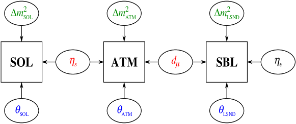
Figure 1: Convenient separation of parameter dependence of the different data sets used in Refs. Maltoni:2001bc , Maltoni:2002xd .

We will adopt this generalized framework in the description of solar and atmospheric oscillations Maltoni:2002ni presented in Secs. 3.1 and 3.2 where we describe, in particular, the constraints implied by both solar and atmospheric data samples on the sterile admixture, $\eta_{s}$. On the other hand this parametrization will also be employed in the global analysis Maltoni:2002xd of all current oscillation data presented in Sec. 3.5.

2.2 The Absolute Scale of Neutrino Mass

Neutrino oscillations are sensitive only to mass splittings, not to the absolute scale of neutrino mass. Probing the latter requires either direct kinematical tests, using tritium beta spectrometers katrin , or observations of the Cosmic Microwave Background and large scale structure, sensitive to a sub-leading hot dark matter component Elgaroy:2002bi . The present limits come from a long list of painstaking efforts to study neutrino mass effects in beta decays, which culminated with the Mainz and Troitsk results (see Ref. katrin for the corresponding references). Given the smallness of the solar and atmospheric mass splittings, the resulting (conservative) bounds on the sum of all neutrino masses Elgaroy:2002bi , pdg are illustrated in the ordinate of Fig. 3.

To decide whether neutrinos are Dirac or Majorana particles requires the investigation of $\Delta L=2$ (L denoting lepton-number) processes, of which $\beta\beta_{0\nu}$ decay provides the most classic example Morales:1998hu . Indeed, there is a black-box theorem Schechter:1981bd stating that, in a “natural” gauge theory, the observation of this process would signify the discovery that neutrinos are, as expected by theory Schechter:1980gr , Majorana fermions. This connection is illustrated by Fig. 2.

Figure 2: The black-box $\beta\beta_{0\nu}$ argument Schechter:1981bd .

The importance of this simple argument lies in its generalality: it holds irrespective of how $\beta\beta_{0\nu}$ is engendered. However, in order to quantify its implications, one needs to specify the particular model.

In the neutrino-exchange-induced mechanism, $\beta\beta_{0\nu}$ is characterized by an “effective” neutrino mass parameter $M_{ee}$ whose value is sensitive to possible cancellations among individual neutrino amplitudes. These may arise either as a result of symmetries pseudo , QDN or due to the Majorana-type $CP$ phases Schechter:1980gr . Nevertheless one can show that Barger:2002xm , as illustrated in Fig. 3, there is a direct correlation between $M_{ee}$ and the neutrino mass scales probed in tritium beta decays pdg and cosmology Elgaroy:2002bi . It is therefore important to probe $\beta\beta_{0\nu}$ in a more sensitive experiment Klapdor-Kleingrothaus:1999hk .

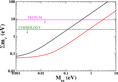
Figure 3: $\beta\beta_{0\nu}$ and the scale of neutrino mass.

3 Neutrino Oscillations

Although the three-active neutrino oscillation scheme gives a good description of both solar and atmospheric data, we will follow the approach given in Ref. Maltoni:2002ni in which they are analysed in terms of mixed active-sterile neutrino oscillations. Such generalized scheme has as advantages that it allows one to systematically combine solar and atmospheric data with the current short baseline neutrino oscillation data samples including the LSND evidence for oscillations Maltoni:2002xd , as done in Sec. 3.5. This is justified, since current reactor bounds on $\theta_{13}$ (Sec. 3.3.1) are stronger than solar and atmospheric bounds on the parameter $\eta_{s}$ (with $0\leq\eta_{s}\leq 1$, see Secs. 3.1 and 3.2) describing the fraction of sterile neutrinos taking part in the solar oscillations. By taking such simplified analysis with $\theta_{13}\to 0$, we completely decouple the solar and atmospheric oscillations from each other, and comply trivially with the strong constraints from reactor experiments. For a complementary earlier analysis with $\theta_{13}\neq 0$ effects, but no sterile neutrinos, see Ref. 3-nu-sol+atm-fit . As seen in Fig. 1, mixed active-sterile neutrino oscillations are characterized by a total of six mixing angles Schechter:1980gr .

3.1 Solar Neutrinos

The solar neutrino data include the solar neutrino rates of the chlorine experiment Homestake Cleveland:nv ($2.56\pm 0.16\pm 0.16$ SNU), the most recent result of the gallium experiments SAGE Abdurashitov:1999bv  ($70.8~{}^{+5.3}_{-5.2}~{}^{+3.7}_{-3.2}$ SNU) and GALLEX/GNO Altmann:2000ft ($70.8\pm 4.5\pm 3.8$ SNU), as well as the 1496-days Super-Kamiokande data sample Fukuda:2002pe . The latter are presented in the form of 44 bins (8 energy bins, 6 of which are further divided into 7 zenith angle bins). In addition to this, we have the latest results from SNO presented in Refs. Ahmad:2002jz , in the form of 34 data bins (17 energy bins for each day and night period). Therefore, in our statistical analysis there are $3+44+34=81$ observables.

The most popular explanation of solar neutrino experiments is provided by the neutrino oscillations hypothesis. For generality we follow the approach given in Ref. Maltoni:2002ni in which they are analysed in terms of mixed active-sterile neutrino oscillations, where the electron neutrino produced in the sun converts to $\nu_{x}$ (a combination of $\nu_{\mu}$ and $\nu_{\tau}$) and a sterile neutrino $\nu_{s}\>$: $\nu_{e}\to\sqrt{1-\eta_{s}}\,\nu_{x}+\sqrt{\eta_{s}}\,\nu_{s}$.

In such framework the solar neutrino data are fit with three parameters $\Delta m^{2}{sol}$, $\theta{sol}$ and $\eta_{s}$. The parameter $\eta_{s}$ with $0\leq\eta_{s}\leq 1$ describes the fraction of sterile neutrinos taking part in the solar oscillations, so that when $\eta_{s}\to 0$ one recovers the conventional active oscillation case. The main motivation for adopting such generalized scenarios is the possibility of combining the solar and atmospheric data with short baseline oscillations Maltoni:2002xd . Four-neutrino mass schemes Peltoniemi:1992ss are the most natural candidates to accommodate solar and atmospheric mass-splittings with the hint from LSND LSND indicating a large $\Delta m^{2}$, see Sec. 3.3.

In Fig. 4 we display the regions of solar neutrino oscillation parameters for 3 d.o.f. with respect to the global minimum, for the standard case of active oscillations, $\eta_{s}=0$, as well as for $\eta_{s}=0.2$ and $\eta_{s}=0.5$. The first thing to notice is the impact of the SNO NC, spectral, and day-night data in improving the determination of the oscillation parameters: the shaded regions after their inclusion are much smaller than the hollow regions delimited by the corresponding SNO${}_{\mathrm{CC}}^{\mathrm{rate}}$  confidence contours. Especially important is the full SNO${}_{\mathrm{CC,NC}}^{\mathrm{SP,DN}}$  information in closing the LMA-MSW region from above: values of $\Delta m^{2}{sol}>10^{-3}~{}\rm{eV}^{2}$ appear only at $3\sigma$. Previous solar data on their own could not close the LMA-MSW region, only the inclusion of reactor data CHOOZ probed the upper part of the LMA-MSW region 3-nu-sol+atm-fit . Furthermore, the complete SNO${}_{\mathrm{CC,NC}}^{\mathrm{SP,DN}}$  information is important for excluding maximal solar mixing in the LMA-MSW region. At $3\sigma$ with 1 d.o.f.  one has

$$\rm{LMA-MSW:}\quad 0.26\leq\tan^{2}\theta{sol}\leq 0.85\,,\quad 2.6\times 10^{-5}~{}\rm{eV}^{2}\leq\Delta m^{2}{sol}\leq 3.3\times 10^{-4}~{}\rm{eV}^{2}$$ (1)

showing that in the LMA-MSW region $\tan^{2}\theta{sol}$ is significantly below maximal.

Note that in order to compare the allowed regions in Fig. 4 with others Lisi , one must note that our C.L. regions correspond to the 3 d.o.f. corresponding to $\tan^{2}\theta{sol}$, $\Delta m^{2}{sol}$ and $\eta_{s}$. Therefore at a given C.L. our regions are larger than the usual regions for 2 d.o.f., because we also constrain the parameter $\eta_{s}$.

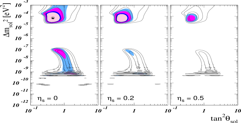
Figure 4: Allowed $\tan^{2}\theta{sol}$ and $\Delta m^{2}{sol}$ regions for $\eta_{s}=0$ (active oscillations), $\eta_{s}=0.2$ and $\eta_{s}=0.5$. The lines and shaded regions correspond to the SNO${}_{\mathrm{CC}}^{\mathrm{rate}}$  and SNO${}_{\mathrm{CC,NC}}^{\mathrm{SP,DN}}$ analyses, respectively, as defined in Ref. Maltoni:2002ni . The 90%, 95%, 99% C.L. and 3$\sigma$ contours are for 3 d.o.f..

Our global best fit point occurs for active oscillations with

$$\rm{LMA-MSW:}\quad\tan^{2}\theta{sol}=0.46\,,\quad\Delta m^{2}{sol}=6.6\times 10^{-5}~{}\rm{eV}^{2}$$ (2)

A concise way to illustrate the above results is displayed in Fig. 5. We give the profiles of $\Delta\chi^{2}{sol}$ as a function of $\Delta m^{2}{sol}$ (left), $\tan^{2}\theta{sol}$ (middle) as well as $\eta_{s}$ (right), by minimizing with respect to the undisplayed oscillation parameters. In the left and middle panels the solid, dashed and dot-dashed lines correspond to $\eta_{s}=0$, $\eta_{s}=1$ and $\eta_{s}=0.5$, respectively.

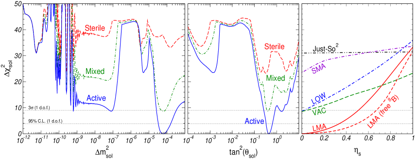
Figure 5: $\Delta\chi^{2}{sol}$ as a function of $\Delta m^{2}{sol}$, $\tan^{2}\theta{sol}$, and $0\leq\eta_{s}\leq 1$ from global SNO${}_{\mathrm{CC,NC}}^{\mathrm{SP,DN}}$  sample defined in Ref. Maltoni:2002ni .

The use of the full SNO${}_{\mathrm{CC,NC}}^{\mathrm{SP,DN}}$  sample has lead to the relative worsening of all oscillation solutions with respect to the preferred active LMA-MSW solution. One sees also how the preferred status of the LMA-MSW solution survives in the presence of a small sterile admixture characterized by $\eta_{s}$. Increasing $\eta_{s}$ leads to a deterioration of all oscillation solutions. Note that in the right panel we display the profile of $\Delta\chi^{2}{sol}$ as a function of $0\leq\eta_{s}\leq 1$, irrespective of the detailed values of the solar neutrino oscillation parameters $\Delta m^{2}{sol}$ and $\theta{sol}$. One can see that there is a crossing between the LMA-MSW and VAC solutions. This implies that the best pure–sterile description lies in the VAC regime. However, in the global analysis pure sterile oscillations with $\eta_{s}=1$ are highly disfavored. The $\chi^{2}$-difference between pure active and sterile is $\Delta\chi^{2}_{\mathrm{s-a}}=32.2$ if one restricts to the LMA-MSW solution, or $\Delta\chi^{2}_{\mathrm{s-a}}=23.3$ if one also allows for VAC. For 3 d.o.f. the $\Delta\chi^{2}_{\mathrm{s-a}}=23.3$ implies that pure sterile oscillations are ruled out at 99.997% C.L. compared to the active case.

For the LMA-MSW solution one can also perform an analysis without fixing the boron flux to its SSM prediction, as seen in the right panel of Fig. 5. One can see that in this case the constraint on $\eta_{s}$ is weaker than in the boron-fixed case, since a small sterile component can now be partially compensated by increasing the total boron flux coming from the Sun. From the figure one obtains the bounds

$$\rm{solar\>\>data:}\quad\eta_{s}\leq 0.44\rm{~{}(boron-fixed)},\quad\eta_{s}\leq 0.61\rm{~{}(boron-free)}$$ (3)

at 99% C.L. for 1 d.o.f.. A complete table of best fit values of $\Delta m^{2}{sol}$ and $\theta{sol}$ with the corresponding $\chi^{2}{sol}$ and GOF values for pure active, pure sterile, and mixed neutrino oscillations is given in Ref. Maltoni:2002ni , both for the SNO${}_{\mathrm{CC}}^{\mathrm{rate}}$  ($48-2$ d.o.f.) and the SNO${}_{\mathrm{CC,NC}}^{\mathrm{SP,DN}}$  analysis ($81-2$ d.o.f.).

Comparing different solar neutrino analyses

Table 1 summarizes a compilation of the results of the solar neutrino analyzes performed by the SNO and Super–K collaborations, as well as by different theoretical groups (see Ref. Maltoni:2002ni for the references). All groups find the best fit in the LMA-MSW region, although there are quantitative differences even for this preferred solution. As can be seen from the table, the GOF of the best-fit LMA-MSW solution, ranges from 53% to 97%.

Generally speaking, one expects the differences in the statistical treatment of the data to have little impact on the global best fit point, located in the LMA-MSW region. These differences typically become more visible as one compares absolute $\chi^{2}$ values or departs from the best fit region towards more disfavored solutions. Aware of this, Ref. Maltoni:2002ni took special care to details such as the dependence of the theoretical errors on the oscillation parameters entering the covariance matrix characterizing the Super-K and SNO electron recoil spectra. This ensures reliability of the results in the full $\tan^{2}\theta{sol}$-$\Delta m^{2}{sol}$ plane.

The row labeled “d.o.f.” in table 1 gives the number of analyzed data points minus the fitted parameters in each analysis. We also present the best fit values of $\tan^{2}\theta{sol}$ and $\Delta m^{2}{sol}$ for active oscillations, the corresponding $\chi^{2}$-minima and GOF, as well as the $\Delta\chi^{2}$ with respect to the favored active LMA-MSW solution

	SNO Collaboration	Super–K Collaboration	Barger et al	Bandyopadhyay et al	Bahcall et al	Creminelli et al	Aliani et al	De Holanda & Smirnov	Fogli et al	Barranco et al, Ref. Barranco:2002te	Maltoni et al, Ref. Maltoni:2002ni
d.o.f.	75-3	46	75-3	49-4	80-3	49-2	41-4	81-3	81-3	81-2	81-2
best OSC-fit	active LMA-MSW solution
$\tan^{2}\theta{sol}$	0.34	0.38	0.39	0.41	0.45	0.45	0.40	0.41	0.42	0.47	0.46
$\Delta m^{2}{sol}$ [$10^{-5}$ eV2]	5.0	6.9	5.6	6.1	5.8	7.9	5.4	6.1	5.8	5.6	6.6
$\chi^{2}_{\mathrm{\bf LMA}}$	57.0	43.5	50.7	40.6	75.4	33.0	30.8	65.2	73.4	68.0	65.8
GOF	90%	58%	97%	66%	53%	94%	80%	85%	63%	81%	86%
$\Delta\chi^{2}_{\rm{\bf LOW}}$	10.7	09.0	09.2	10.0	09.6	08.1	–	12.4	10.0	–	08.7
$\Delta\chi^{2}_{\rm{\bf VAC}}$	–	10.0	25.6	15.5	10.1	14.0	–	09.7	07.8	–	08.6
$\Delta\chi^{2}_{\rm{\bf SMA}}$	–	15.4	57.3	30.4	25.6	23.0	–	34.5	23.5	–	23.5

Table 1: Comparison of different solar neutrino analyzes before KamLAND, from Ref. Maltoni:2002ni . See text.

One can see from these numbers how various groups use different experimental input data, in particular the spectral and zenith angle information of Super–K and/or SNO. Despite differences in the analyzes there is relatively good agreement on the best fit active LMA-MSW parameters: the best fit values for $\tan^{2}\theta{sol}$ are in the range $0.34-0.47$ and for $\Delta m^{2}{sol}$ they lie in the range $(5.0-7.9)\times 10^{-5}$ eV². There is also good agreement on the allowed ranges of the oscillation parameters (not shown in the table). For example, the $3\sigma$ intervals given in Bahcall et al ($0.24\leq\tan^{2}\theta{sol}\leq 0.89,\>2.3\times 10^{-5}\>\rm{eV}^{2}\leq\Delta m^{2}{sol}\leq 3.7\times 10^{-4}\>\rm{eV}^{2}$) and Holanda-Smirnov ($\tan^{2}\theta{sol}\leq 0.84,\>2.3\times 10^{-5}\>\rm{eV}^{2}\leq\Delta m^{2}{sol}\leq 3.6\times 10^{-4}\>\rm{eV}^{2}$) agree very well with those given in Ref. Maltoni:2002ni . There is remarkable agreement on the rejection of the LOW solution with respect to LMA-MSW with a $\Delta\chi^{2}_{\rm{LOW,active}}\approx 10$. The result for the vacuum solution in Maltoni:2002ni $\Delta\chi^{2}_{\rm{VAC,active}}=8.6$ is in good agreement with the values obtained by the Super-K collaboration, as well as Bahcall et al, de Holanda & Smirnov and Fogli et al, whereas Bandyopadhyay et al, Barger et al and Creminelli et al obtain higher values. For the SMA-MSW solution one finds $\Delta\chi^{2}_{\rm SMA,active}=23.5$, in good agreement with the values obtained in Bahcall et al, Creminelli et al and Fogli et al; while Bandyopadhyay et al and de Holanda & Smirnov, and especially Barger et al, obtain higher values. Typically the results of a given analysis away from the best fit LMA-MSW region serve as an indicator of its quality.

All in all, in view of the vast input data, of possible variations in the choice of the $\chi^{2}$ function and the treatment of errors and their correlations, and of the complexity of the codes involved, it is encouraging that there is reasonable agreement amongst different analyzes, especially for the LMA-MSW solution. As shown in Sec. 3.4, LMA-MSW is now strongly preferred after the results of KamLAND described in Sec. 3.3.2. From this point of view it has now become somewhat academic to scrutinize further the origin of the differences found in the various analyses. Nature has chosen the simplest solution.

3.2 Atmospheric Neutrinos

Here we summarize the analysis of atmospheric data given in a generalized oscillation scheme in which a light sterile neutrino takes part in the oscillations Maltoni:2002ni . For simplicity the approximation $\Delta m^{2}{sol}\ll\Delta m^{2}{atm}$ is used and the electron neutrino is taken as completely decoupled from atmospheric oscillations, by setting $\theta_{13}\to 0$ (for an analysis with $\theta_{13}\neq 0$ see 3-nu-sol+atm-fit ). This way we comply with the strong constraints from reactor experiments in Sec 3.3.1. In contrast with the case of solar oscillations, the constraints on the $\nu_{\mu}$–content in atmospheric oscillations are not so stringent. Thus the description of atmospheric neutrino oscillations in this general framework requires two new parameters besides the standard two-neutrino oscillation parameters $\theta{atm}$ and $\Delta m^{2}{atm}$. The parameters $d_{\mu}$ and $d_{s}$ introduced in Ref. Maltoni:2001bc and illustrated in Fig. 1 are defined in such a way that $1-d_{\mu}$ ($1-d_{s}$) corresponds to the fraction of $\nu_{\mu}$ ($\nu_{s}$) participating in oscillations with $\Delta m^{2}{atm}$. Hence, pure active atmospheric oscillations with $\Delta m^{2}{atm}$ are recovered when $d_{\mu}=0$ and $d_{s}=1$. In four-neutrino models there is a mass-scheme-dependent relationship between $d_{s}$ and the solar parameter $\eta_{s}$. For details see Ref. Maltoni:2001bc .

To get a feeling on the physical meaning of these two parameters, note that for $d_{\mu}=0$ the $\nu_{\mu}$ oscillates with $\Delta m^{2}{atm}$ to a linear combination of $\nu_{\tau}$ and $\nu_{s}$ given as $\nu_{\mu}\to\sqrt{d_{s}}\,\nu_{\tau}+\sqrt{1-d_{s}}\,\nu_{s}\,.$ For earlier pure active descriptions see, for example, Refs. Fornengo:2001pm , Fornengo:2000sr and papers therein.

The global best fit point occurs at

$$\sin^{2}\theta{atm}=0.49\,,\quad\Delta m^{2}{atm}=2.1\times 10^{-3}~{}\rm{eV}^{2}$$ (4)

and has $d_{s}=0.92,\>d_{\mu}=0.04$. One sees that atmospheric data prefers a small sterile neutrino admixture. However, this is not statistically significant, since the pure active case ($d_{s}=1,d_{\mu}=0$) also gives an excellent fit: the difference in $\chi^{2}$ with respect to the best fit point is only $\Delta\chi^{2}_{\mathrm{act-best}}=3.3$. For the pure active best fit point one obtains,

$$\sin^{2}\theta{atm}=0.5\,,\>\Delta m^{2}{atm}=2.5\times 10^{-3}~{}\rm{eV}^{2}\>$$ (5)

with the 3$\sigma$ ranges (1 d.o.f.)

$$0.3\leq\sin^{2}\theta{atm}\leq 0.7$$ (6)

$$1.2\times 10^{-3}~{}\rm{eV}^{2}\leq\Delta m^{2}{atm}\leq 4.8\times 10^{-3}~{}\rm{eV}^{2}\,.$$ (7)

The determination of the parameters $\theta{atm}$ and $\Delta m^{2}{atm}$ is summarized in Figs. 6 and 7.

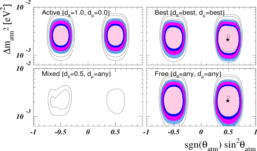
Figure 6: Allowed regions of $\sin^{2}\theta{atm}$ and $\Delta m^{2}{atm}$ at 90%, 95%, 99% and 3$\sigma$ for 4 d.o.f. and different assumptions on the parameters $d_{s}$ and $d_{\mu}$, from Maltoni:2002ni . The lines (shaded regions) correspond to 1289 (1489) days of Super-K data.

Note that Fig. 7 considers several cases: arbitrary $d_{s}$ and $d_{\mu}$, best–fit $d_{s}$ and $d_{\mu}$, and pure active and mixed active–sterile neutrino oscillations, as indicated.

At a given C.L. the $\chi^{2}{atm}$ is cut at a $\Delta\chi^{2}$ determined by 4 d.o.f. to obtain 4-dimensional volumes in the parameter space of ($\theta{atm},\Delta m^{2}{atm},d_{\mu},d_{s}$). In the upper panels we show sections of these volumes at values of $d_{s}=1$ and $d_{\mu}=0$ corresponding to the pure active case (left) and the best fit point (right). Again one sees that moving from pure active to the best fit does not change the fit significantly. In the lower right panel both $d_{\mu}$ and $d_{s}$ are projected away, whereas in the lower left panel $d_{s}=0.5$ is fixed and one eliminates only $d_{\mu}$. Comparing the regions resulting from 1489 days Super-K data (shaded regions) with the one from the 1289 days Super-K sample (hollow regions) we note that the new data leads to a slightly better determination of $\theta{atm}$ and $\Delta m^{2}{atm}$. However, more importantly, from the lower left panel we see how the new data show a much stronger rejection against a sterile admixture: for $d_{s}=0.5$ no allowed region appears at 3$\sigma$ for 4 d.o.f..

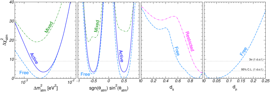
Figure 7: $\Delta\chi^{2}{atm}$ as a function of $\Delta m^{2}{atm}$, $\sin^{2}\theta{atm}$, $d_{s}$ and $d_{\mu}$. In each panel the undisplayed parameters are integrated out. The “Mixed” and “Restricted” cases correspond to $d_{s}=0.5$ and $d_{\mu}=0$, respectively Maltoni:2002ni .

The excellent quality of the neutrino oscillation description of the present atmospheric neutrino data can be better appreciated by displaying the zenith angle distribution of atmospheric neutrino events, given in Fig. 8.

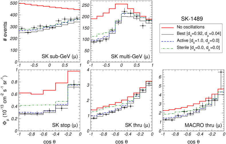
Figure 8: Zenith angle dependence of the $\mu$-like atmospheric neutrino data from Ref. Maltoni:2002ni . The predicted number of atmospheric neutrino events for best–fit, pure–active and pure–sterile oscillations and no oscillations are given, for comparison.

Clearly, active neutrino oscillations describe the data very well indeed. In contrast, the no-oscillations hypothesis can be visually spotted as being ruled out. On the other hand, conversions to sterile neutrinos lead to an excess of events for neutrinos crossing the core of the Earth, in all the data samples except sub-GeV.

3.3 Reactor and Accelerator Neutrino Data

3.3.1 Chooz and Palo Verde

The Chooz experiment has been the first relatively long-baseline reactor neutrino experiment. As used in Ref. Maltoni:2001bc , the measured $\bar{\nu}_{e}$ survival probability from these experiments are $P=1.01\pm 0.028\pm 0.027$ for Chooz, and $P=1.01\pm 0.024\pm 0.053$ for Palo Verde CHOOZ . The non-observation of oscillations at these reactors provides an important restriction on $\Delta{m}^{2}_{32}$ and $\sin^{2}(2\theta_{13})$, as illustrated in Fig. 9.

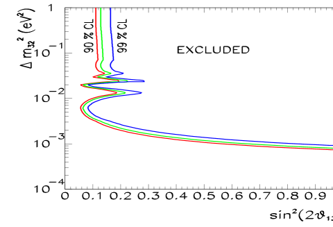
Figure 9: Region in $\Delta{m}^{2}_{32}$ and $\sin^{2}(2\theta_{13})$ excluded by the Chooz reactor, from 3-nu-sol+atm-fit .

The curves represent the 90, 95 and 99% CL excluded region defined with 2 d. o. f. for comparison with the Chooz published results. For large $\Delta{m}^{2}_{32}$ this gives a stringent limit on $\sin^{2}(2\theta_{13})$, but not for low $\Delta{m}^{2}_{32}$ values. Together with atmospheric data this implies that $\theta_{13}$ must be rather small. As will be seen below $\Delta m^{2}{atm}\gg\Delta m^{2}{sol}$, i. e. one has a somewhat hierarchical structure of neutrino mass splittings.

3.3.2 KamLAND

In the KamLAND reactor neutrino experiment the target for the $\bar{\nu}_{e}$ flux consists of a spherical transparent balloon filled with 1000 tons of non-doped liquid scintillator. The anti-neutrinos are detected via the inverse neutron $\beta$-decay

$$\bar{\nu}_{e}+p\to e^{+}+n\,.$$ (8)

The spectral data are given in 13 bins of prompt energy above 2.6 MeV in Fig. 5 of Ref. :2002dm .

There have been already several papers analysing the first results of the KamLAND experiment, here we follow Ref. Maltoni:2002aw . The KamLAND data are simulated by calculating the expected number of events in each bin for given oscillation parameters as

$$N_{i}^{\mathrm{th}}(\Delta m^{2},\theta)=f\int dE_{\nu}\sigma(E_{\nu})\\ \sum_{j}\phi_{j}(E_{\nu})P_{j}(E_{\nu},\Delta m^{2},\theta)\int_{i}dE_{e}R(E_{e},E^{\prime}_{e})\,.$$ (9)

Here $R(E_{e},E_{e}^{\prime})$ is the energy resolution function and $E_{e},E_{e}^{\prime}$ are the observed and the true positron energy, respectively, and an energy resolution of $7.5\%/\sqrt{E(\mathrm{MeV})}$ is assumed :2002dm . The neutrino energy is related to the positron energy by $E_{\nu}=E_{e}^{\prime}+\Delta$, where $\Delta$ is the neutron-proton mass difference. The integration interval over $E_{e}$ is determined by the prompt energy interval in each bin. The neutrino spectrum $\phi(E_{\nu})$ from nuclear reactors is well known, the phenomenological parameterization given in Refs. Vogel:iv , Murayama:2000iq has been used. The average fuel composition for the nuclear reactors given in Ref. :2002dm is adopted and possible effects due to time variations in the fuel composition have been neglected Murayama:2000iq . The sum over $j$ in Eq. (9) runs over 16 nuclear plants, taking into account the different distances from the detector and the power output of each reactor (see Table 3 of Ref. kamlandproposal ). The relevant detection cross section $\sigma(E_{\nu})$ is given in Ref. Vogel:1999zy . In the two-neutrino framework the disappearance probability for the neutrinos coming from the reactor $j$ is given by

$$P_{j}(E_{\nu},\Delta m^{2},\theta)=1-\sin^{2}2\theta\sin^{2}\frac{\Delta m^{2}L_{j}}{4E_{\nu}}\,.$$ (10)

The normalization factor $f$ in Eq. (9) is determined in such a way that for the case of no oscillations the total number of events is 86.8, as expected from the Monte-Carlo simulation used in Ref. :2002dm .

For the statistical analysis one uses the $\chi^{2}$-function

$$\chi^{2}=\sum_{i,j}(N_{i}^{\mathrm{th}}-N_{i}^{\mathrm{obs}})S^{-1}_{ij}(N_{j}^{\mathrm{th}}-N_{j}^{\mathrm{obs}})\,.$$ (11)

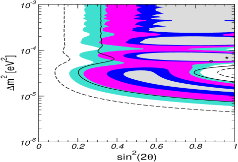
Figure 10: Allowed regions at 90%, 95%, 99% and 99.73% C.L. (2 d.o.f.) from KamLAND spectral data. The solid (dashed) line is the 95% C.L. ($3~{}\sigma$) region from the KamLAND rate alone. The star (dot) is the best fit point from the spectral (rate) analysis, from Ref. Maltoni:2002aw .

The observed number of events $N_{j}^{\mathrm{obs}}$ in each bin can be read off from Fig. 5 of Ref. :2002dm . In the covariance matrix one includes the statistical errors (obtained from the same figure) and the systematic error implied by the 6.42% uncertainty on the total number of events expected for no oscillations :2002dm .

In Fig. 10 we show the allowed regions of the oscillation parameters obtained from our re-analysis of the KamLAND data. It is in good agreement with the analysis performed by the KamLAND collaboration, shown in Fig. 6 of Ref. :2002dm . After this successful calibration we turn to a full global analysis combining also with the solar data sample of Sec. 3.4.

3.3.3 K2K

Further evidence for the atmospheric neutrino anomaly has now come from the K2K experiment Ahn:2002up using accelerator neutrinos in a long-baseline set-up. The collaboration sees a reduction of the $\nu_{\mu}$ flux together with a distortion of the energy spectrum. They observe 56 beam neutrino events 250 km away from the neutrino production point, with an expectation of $80.1^{+6.2}_{-5.4}$. They also reconstruct the neutrino energy spectrum, which fits better the expected shape with neutrino oscillation than without. The probability that the observed flux at Super-K is a statistical fluctuation without neutrino oscillation is less than 1%.

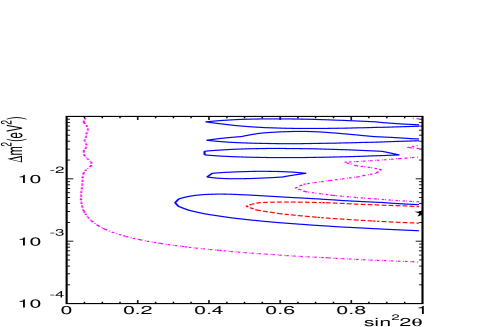
Figure 11: Allowed regions of oscillation parameters from the K2K data of Ref. Ahn:2002up . Dashed, solid and dot-dashed lines are 68.4%, 90% and 99% C.L. contours, respectively. The best fit point is indicated by the star.

The collaboration performs a two-neutrino oscillation analysis, with $\nu_{\mu}$ disappearance, using the maximum-likelihood method, and including both the number of events and the energy spectrum shape. The results are given in Fig. 11 and agree nicely with what is inferred from the atmospheric analysis, Sec. 3.2.

3.3.4 LSND

The Liquid Scintillating Neutrino Detector (LSND) is an experiment designed to search for neutrino oscillations in appearance channels. It is the only short baseline accelerator neutrino experiment claiming evidence for oscillations.

Here we compare the implications of two different analyses of the LSND data. The first uses the likelihood function obtained in the final LSND analysis LSND from their global data with an energy range of $20<E_{e}<200$ MeV and no constraint on the likelihood ratio $R_{\gamma}$ (see Ref. LSND for details). This sample contains 5697 events including decay-at-rest (DAR) $\bar{\nu}_{\mu}\to\bar{\nu}_{e}$, and decay-in-flight (DIF) $\nu_{\mu}\to\nu_{e}$ data. We refer to this analysis as LSND global. The second corresponds to the LSND analysis performed in Ref. Church:2002tc based on 1032 events obtained from the energy range $20<E_{e}<60$ MeV and applying a cut of $R_{\gamma}>10^{-5}$. These cuts eliminate most of the DIF events from the sample, leaving mainly the DAR data, which are more sensitive to the oscillation signal. We refer to this analysis as LSND DAR.

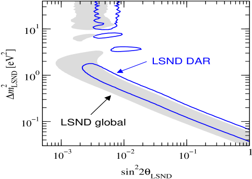
Figure 12: Comparison of the 99% C.L. regions of the global LSND analysis LSND (shaded region) and of the analysis in Ref. Church:2002tc (solid line) using the decay-at-rest (DAR) sample. From Ref. Maltoni:2002xd

In both cases the likelihood function obtained in the analyses of the LSND collaboration was used and this was converted into a $\chi^{2}$ according to $\chi^{2}\propto-2\ln\mathcal{L}$ (see Ref. Maltoni:2001bc for details). In Fig. 12 we compare the 99% C.L. regions obtained from the two LSND analyses. The LSND DAR data prefers somewhat larger mixing angles, which will lead to a stronger disagreement of the data in (3+1) oscillation schemes (see below). Furthermore, the differences in $\chi^{2}$ between the best fit point and no oscillations for the two analyses are given by $\Delta\chi^{2}_{\mathrm{no\,osc}}=29$ (global) and $\Delta\chi^{2}_{\mathrm{no\,osc}}=47$ (DAR). This shows that the information leading to the positive oscillation signal seems to be more condensed in the DAR data. Note that the detailed information from the short baseline disappearance no-evidence experiments Bugey bugey and CDHS CDHS has been fully taken into account. Concerning the constraints from KARMEN KARMEN , they are included by means of the KARMEN likelihood function.

3.4 Neutrino Oscillations After KamLAND

There has been a rush of recent papers on the analysis of neutrino data after KamLAND in the framework of the neutrino oscillation hypothesis (assuming, of course, $CPT$ invariance) Maltoni:2002aw , kamland02others . Here we discuss the results of the analysis presented in Ref. Maltoni:2002aw , to which the reader is referred for the details. Figs. 13 and 14 summarize the results obtained in a combined fit of the full KamLAND data sample with the global sample of solar neutrino data (the same as used in Ref. Maltoni:2002ni ), as well as the Chooz result.

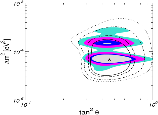
Figure 13: Allowed regions at 90%, 95%, 99% and 99.73% C.L. (2 d.o.f.) from the combined analysis of solar, Chooz and KamLAND data. The hollow lines are the allowed regions from solar and Chooz data alone. The star (dot) is the best fit point from the combined (solar+Chooz only) analysis from Ref. Maltoni:2002aw .

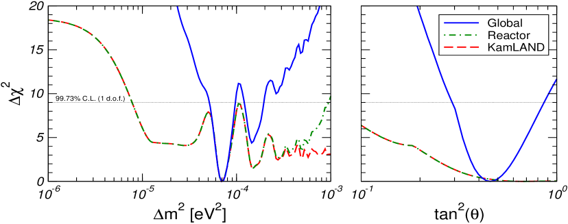
Figure 14: $\Delta\chi^{2}$ versus $\Delta m^{2}{sol}$ and $\tan^{2}\theta$. The red dashed line refers to KamLAND alone. The green dot-dashed line corresponds to the full reactor data sample, including both KamLAND and Chooz. The blue solid line refers to the global analysis of the complete solar and reactor data, from Ref. Maltoni:2002aw .

First of all, we have quantified the rejection of non-LMA solutions and found that it is now more robust. For example, for the LOW solution one has $\Delta\chi^{2}=26.9$, which for 2 d.o.f. ($\Delta m^{2}{sol}$ and $\theta$) lead to a relative probability of $1.4\times 10^{-6}$. A similar result is also found for the VAC solution. Besides selecting out LMA-MSW as the unique solution of the solar neutrino problem we find, however, that the new reactor results have little impact on the location of the best fit point:

$$\tan^{2}\theta=0.46,\qquad\Delta m^{2}{sol}=6.9\times 10^{-5}~{}\rm{eV}^{2}.$$ (12)

In particular the solar neutrino mixing remains significantly non-maximal, a point which is not in conflict with the fact that KamLAND data alone prefer maximal mixing :2002dm , since this has no statistical significance Maltoni:2002aw . Indeed, one can see from the right panel in Fig. 14 that $\Delta\chi^{2}$ is rather flat with respect to the mixing angle for $\tan^{2}\theta\raise 1.29167pt\hbox{$\;>$\kern-7.5pt\raise-4.73611pt\hbox{$\sim\;$}}0.4$. This explains why the addition of the KamLAND data has no impact whatsoever in the determination of the solar neutrino oscillation mixing. The allowed $3\sigma$ region one finds for $\theta$ is:

$$0.29\leq\tan^{2}\theta\leq 0.86,$$ (13)

essentially the same as the pre-KamLAND range given in Eq. (1).

Note that the solar mixing angle is large, but significantly non-maximal, in contrast to the atmospheric mixing, Eq. (5). This important fact implies that models where the solar mixing is non-maximal Babu:2002dz are strongly preferred over bi-maximal mixing models Chankowski:2000fp .

Turning to the solar neutrino mass splittings, the new data do have a strong impact in narrowing down the allowed $\Delta m^{2}{sol}$ range. From the left panel of Fig. 14 one can see that the KamLAND data alone provides the bound $\Delta m^{2}{sol}>8\times 10^{-6}~{}\rm{eV}^{2}$, whereas the CHOOZ experiment gives $\Delta m^{2}{sol}<10^{-3}~{}\rm{eV}^{2}$, both at $3\sigma$. Hence global reactor neutrino data provide a robust allowed $\Delta m^{2}{sol}$ range, based only on terrestrial experiments. However, combining this information from reactors with the solar neutrino data leads to a significant reduction of the allowed range: As clearly visible in Fig. 13, the pre-KamLAND LMA-MSW region is now split into two sub-regions. At $3\sigma$ (1 dof.) one obtains

$$5.1\times 10^{-5}~{}\rm{eV}^{2}\leq\Delta m^{2}{sol}\leq 9.7\times 10^{-5}~{}\rm{eV}^{2},\\ 1.2\times 10^{-4}~{}\rm{eV}^{2}\leq\Delta m^{2}{sol}\leq 1.9\times 10^{-4}~{}\rm{eV}^{2}.$$ (14)

This remaining ambiguity might be resolved when more KamLAND data have been collected Murayama:2000iq , deGouvea:2001su , Barger:2000hy .

3.5 Combining LSND Data with the Rest

A possible confirmation of the LSND anomaly would have remarkable implications. The most obvious would be the need for a sterile neutrino, which should be light enough to participate in the oscillations Peltoniemi:1992ss . There are two classes of four-neutrino models, (3+1) and (2+2): in the first the sterile neutrino can decouple from both solar and atmospheric oscillations, while in the more symmetric (2+2) schemes, it can not decouple from both sectors simultaneously Maltoni:2001bc . As a result (2+2) schemes are now more severely rejected by a global analysis .

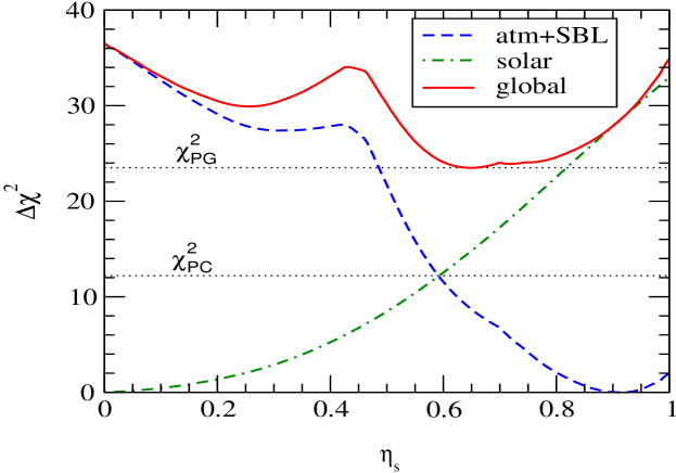
Figure 15: Excluding joint (2+2) oscillation descriptions of current neutrino data including LSND, from Ref. Maltoni:2002xd .

Fig. 15 shows the profiles of $\Delta\chi^{2}{sol}$, $\Delta\chi^{2}_{\mathsc{atm}+\mathsc{sbl}}$ and $\bar{\chi}^{2}_{\mathrm{global}}$ as a function of $\eta_{s}$ in (2+2) oscillation schemes, as well as the values $\chi^{2}_{\mathrm{PC}}$ and $\chi^{2}_{\mathrm{PG}}$ relevant for the parameter consistency and parameter g.o.f. tests proposed in Ref. Maltoni:2002xd .

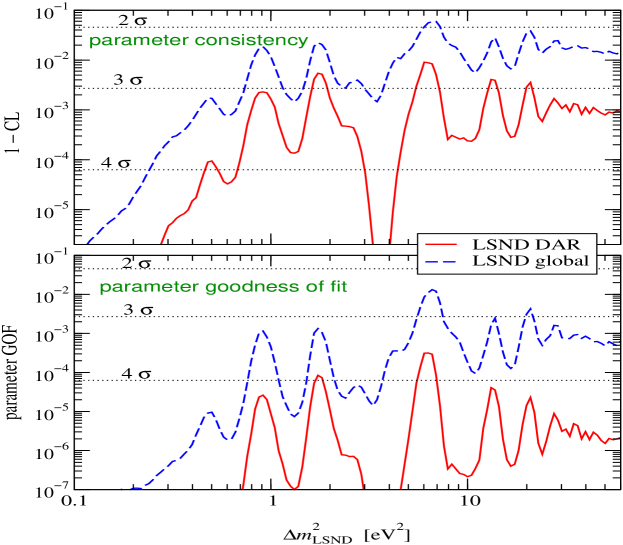
Figure 16: Compatibility of LSND with solar+atmospheric+NEV data in (3+1) schemes, from Ref. Maltoni:2002xd .

The application of these tests to quantify the compatibility of LSND data with the remaining neutrino oscillation data in (3+1) schemes is illustrated in Fig.16. In the upper panel of Fig.16 we show the C.L. of the parameter consistency, whereas in the lower panel we show the parameter g.o.f. for fixed values of $\Delta m^{2}{lsnd}$. The analysis is performed both for the global LSND and for the DAR Church:2002tc LSND data samples. One sees that there is a slim chance to reconcile LSND data with the remaining data, provided $\Delta m^{2}{lsnd}$ is close to 6 eV² or so, but only at the expense of having a rather poor description.

In conclusion one finds that, though 4-neutrino models can not be ruled out per se, the resulting global description of current neutrino oscillation data is extremely poor, even in the case of (3+1) schemes Maltoni:2002xd . We can only wait eagerly for news from the upcoming MiniBooNE experiment. Fortunately this experiment has began collecting data in the last summer. If it turns out that MiniBooNE ultimately confirms the LSND claim we will face a real challenge.

4 Neutrino Mixing in Cosmology and Astrophysics

Neutrino flavour mixing usually has no observational consequences in Cosmology Dolgov:2002wy because in the standard cosmological model all three neutrino flavours were produced in the early universe with identical spectra, and thus with the same energy and number densities. However, it could be that any of the neutrino chemical potentials was initially non-zero, or equivalently that a relic asymmetry between neutrinos and antineutrinos existed, which in turn increases the neutrino energy density and constitutes an extra radiation density. Only mild bounds on neutrino asymmetries exist from the analysis of CMBR anisotropies, while Primordial Big Bang Nucleosynthesis (BBN) places a more restrictive limit on the electron neutrino chemical potential, because the $\bar{\nu}_{e}$ participates directly in the beta processes that determine the primordial neutron-to-proton ratio.

As seen in Sec. 3.4, the KamLAND data have essentially fixed that neutrino oscillations explain the Solar Neutrino Problem with parameters in the LMA-MSW region. It was shown in Ref. Dolgov:2002ab that this result, combined with the evidence of oscillations of atmospheric neutrinos, implies that effective flavour equilibrium is established between all active neutrino species before BBN. Therefore the BBN constraints on the electron neutrino asymmetry apply to all flavours, which in turn implies that neutrino asymmetries do not significantly contribute to the extra relativistic degrees of freedom. Thus the number density of relic neutrinos is very close to its standard value, in such a way that future measurements of the absolute neutrino mass scale, for instance in the forthcoming tritium decay experiment KATRIN katrin , will provide unambiguous information on the cosmic mass density in neutrinos, free of the uncertainty of neutrino chemical potentials.

If non-active light neutrino species exist, as suggested by the LSND data, then they are resrticted also by BBN Lisi:1999ng . However, this is less relevant now that the terrestrial data themselves disfavor the light sterile neutrino oscillation hypothesis.

Back to three-neutrinos, the effect of large solar neutrino mixing in astrophysics can be more substantial. First we note that the large solar mixing angle opens the possibility of probing the noisy character of the deep solar interior Burgess:2002we , especially if an improved determination of $\Delta m^{2}{sol}$ is available from further KamLAND data.

Turning now to supernova neutrino spectra Keil:2002in , LMA-MSW neutrino conversions in a supernova environment induce a significant deformation of the energy spectra of neutrinos Smirnov:ku . Despite this fact, a global analysis of SN1987A and solar neutrino observations establishes the consistency of the LMA-MSW solution Kachelriess:2001sg .

Nevertheless, the large solar mixing angle does have a strong impact on strategies for diagnosing collapse-driven supernovae through neutrino observations, opening new ways to probe supernova parameters. Indeed, fixing the LMA-MSW solution, one may in the future probe otherwise inaccessible features of supernova neutrino spectra such as the temperatures and luminosities of non-electron flavor neutrinos Minakata:2001cd . This can be done simply by observing $\bar{\nu}_{e}$’s from galactic supernovae through the charged current reactions on protons, using massive water Cherenkov detectors. As an illustration we present Fig. 17 different 3 $\sigma$ contours for Super-K and Hyper-K, calculated both for the case of LMA-MSW conversions and no-oscillations. Best fits are indicated by the stars. The plots result from a simulation which uses $\langle E_{\bar{\nu}_{e}}^{0}\rangle=15$ MeV, $\tau^{0}$ = 1.4 and $E_{b}^{0}=3\times 10^{53}$ erg as input supernova parameters. Details in Ref. Minakata:2001cd .

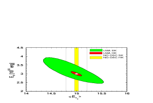
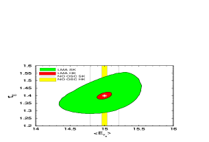
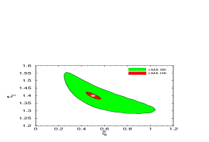
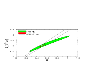
Figure 17: Probing supernova spectra through LMA-MSW oscillations, from Ref. Minakata:2001cd

Recent simulations indicate, however, that although the value of $\tau^{0}$ may be substantially lower than what has been optimistically assumed in Ref. Minakata:2001cd , the fluxes of different flavors of supernova neutrinos may differ Raffelt-pc , giving an additional handle on the diagnostic of supernovae through neutrino observations.

In addition to oscillations, other types of neutrino flavor conversions can affect the propagation of neutrinos in a variety of astrophysical environments, such as supernovae. For example, neutrino non-standard interactions, discussed in Sec. 5, could lead to resonant oscillations of massless neutrinos in matter first-NSI-resonance-paper . These could lead to “deep-inside” conversions Nunokawa:1996tg , rather distinct from those expected from conventional neutrino oscillations Fogli:2002xj .

Another possibility are flavor conversions due to decays of neutrinos, discussed in Sec. 7. If neutrino masses arise from the spontaneous violation of ungauged lepton-number, they are accompanied by a physical Goldstone boson, the majoron seesawmajoron . In the high-density supernova medium the effects of majoron-emitting neutrino decays are important even if they are suppressed in vacuo by small neutrino masses and/or small off-diagonal couplings. Such strong enhancement is due to matter effects, and implies that majoron-emitting decays have an important effect on the neutrino signal of supernovae Kachelriess:2000qc . majoron-neutrino coupling constants in the range $3\times 10^{-7}\raise 1.29167pt\hbox{$\;<$\kern-7.5pt\raise-4.73611pt\hbox{$\sim\;$}}g\raise 1.29167pt\hbox{$\;<$\kern-7.5pt\raise-4.73611pt\hbox{$\sim\;$}}2\times 10^{-5}$ or $g\raise 1.29167pt\hbox{$\;>$\kern-7.5pt\raise-4.73611pt\hbox{$\sim\;$}}3\times 10^{-4}$ are excluded by the observation of SN1987A, and could be probed with improved sensitivity from a future galactic supernova.

5 Non-standard Neutrino Interactions

Non-standard neutrinos interactions (NSI) are a natural feature in most neutrino mass models Schechter:1980gr , fae . They can be of two types: flavour-changing (FC) and non-universal (NU). The co-existence of neutrino masses and NSI in many models of neutrino mass means that neutrino flavor transformations may be induced by both and therefore ideally both should be taken into account when analysing neutrino data.

NSI may be schematically represented as effective dimension-6 terms of the type $\varepsilon G_{F}$, as illustrated in Fig. 18, where $\varepsilon$ specifies their sub-weak strength.

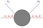
Figure 18: Effective NSI operator.

Such interactions may arise from a nontrivial structure of CC and NC weak interactions characterized a non-unitary lepton mixing matrix and a correspondingly non-trivial NC matrix Schechter:1980gr . Such gauge-induced NSI may lead to flavor and $CP$ violation, even with massless (degenerate) neutrinos NSImodels2 . In radiative models where neutrino mass are “calculable” Zee:1980ai and supersymmetric models with broken R parity Masiero:1990uj , rpmnu-exp FC-NSI can also be Yukawa-induced, from the exchange of spinless bosons. In supersymmetric unified models, NSI may be calculable renormalization effects NSImodels3 . We now describe the impact of non-standard neutrino interactions on solar and atmospheric neutrinos. Since the NSI strengths are highly model-dependent, we treat them as free phenomenological parameters.

5.1 Solar Neutrinos

At the moment one can not yet pin down the exact profile of the $\nu_{e}$ survival probability over the whole spectrum and, as a result, the underlying mechanism of solar neutrino conversion remains unknown. Thus non-oscillation solutions, such as those based on non-standard neutrino matter interactions can be envisaged. As already mentioned, an important feature of the NSI-induced conversions first-NSI-resonance-paper is that the conversion probability is energy-independent. This implies that the solar neutrino energy spectrum is undistorted, as indeed preferred by the Super-K and SNO spectrum data.

In the first paper in Ref. Guzzo:2001mi it has been shown how NSI provide an excellent description of present solar neutrino data. The allowed regions for the NSI mechanism of solar neutrino conversion are shown in Fig. 19. Although the required magnitude of NU interaction is somewhat large, it is not in conflict with current data .

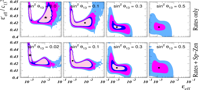
Figure 19: Up-type quark NSI parameters needed to solve the solar neutrino anomaly, from the first of Ref. Guzzo:2001mi .

Moreover one sees that the amount of FC interaction indicated by the best fit is comfortably small.

Such a pure NSI description of solar data with massless and unmixed neutrinos is slightly better than that of the favored LMA-MSW solution, and the NSI values indicated by the solar data analysis do not upset the successful oscillation description of the atmospheric data Guzzo:2001mi . This establishes the overall consistency of a hybrid scheme in which only atmopsheric data are explained in terms of neutrino osciillations. However, the recent first results of the KamLAND collaboration :2002dm reject non-oscillation solutions, such as those based on NSI, at more than 3 $\sigma$ so that the NSI effect in solar neutrino propagation must be sub-leading. Accepting the LMA-MSW solution one may determine restrictions on NSI parametetrs and, therefore, on new aspects of neutrino mass models.

5.2 Atmospheric Neutrinos

Flavor-changing non-standard interactions (FC-NSI) in the $\nu_{\mu}$ -$\nu_{\tau}$ channel have been shown to account for the zenith–angle–dependent deficit of atmospheric neutrinos observed in contained Super-K events Gonzalez-Garcia:1998hj . The solution works even in the absence of neutrino mass and mixing. However such pure NSI explanation fails to reconcile these with Super-K and MACRO up-going muons, due to the lack of energy dependence intrinsic of NSI conversions. The discrepancy is at the 99% C.L. Fornengo:2001pm . Thus, unlike the case of solar neutrinos, the oscillation interpretation of atmospheric data is robust, NSI being allowed only at a sub-leading level. Such robustness of the atmospheric $\nu_{\mu}$ $\to$ $\nu_{\tau}$ oscillation hypothesis can be used to provide the most stringent current limits on FC and NU neutrino interactions, as illustrated in Fig. 20.

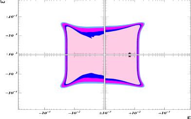
Figure 20: Atmospheric bounds on neutrino NSI with down-type quarks Fornengo:2001pm .

These limits are rather model-independent, as they are obtained from just neutrino-physics processes. As described in Sec. 9.5, future neutrino factories can probing non-standard neutrino interactions in this channel with better sensitivity.

6 Neutrino Magnetic Moments

6.1 Intrinsic Magnetic Moments

Non-zero neutrino masses can manifest themselves through non-standard neutrino electromagnetic properties. When the lepton sector in the Standard Model (SM) is minimally extended as in the quark sector, neutrinos get Dirac masses ($m_{\nu}$) and their magnetic moments (MMs) are tiny MMold ,

$$\mu_{\nu}\simeq 3\times 10^{-19}\mu_{B}\left(\frac{m_{\nu}}{1\,\mathrm{eV}}\right)\,,$$ (15)

where $\mu_{B}$ is the Bohr magneton. Laboratory experiments give 90%C.L. bounds on the neutrino MMs of $1.8\times 10^{-10}\mu_{B}$ rovno and $1.3\times 10^{-10}\mu_{B}$ Li:2002pn , munu for the electron neutrino. These are summarized in Fig. 21.

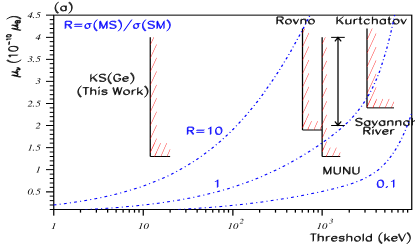
Figure 21: Summary of the results in the searches of neutrino magnetic moments with reactor neutrinos, from Ref. Li:2002pn .

For the muon neutrino the bound is $6.8\times 10^{-10}\mu_{B}$ LSND2 and $3.9\times 10^{-7}\mu_{B}$ for the tau neutrino DONUT (see also Ref. pdg ). On the other hand, astrophysics and cosmology provide limits of the order of $10^{-12}$ to $10^{-11}$ Bohr magnetons Raffelt:gv . Improved sensitivity for the electron neutrino from reactor neutrino searches is expected, while a tritium $\bar{\nu}_{e}$ source experiment H3 aims to reach the level $3\times 10^{-12}\mu_{B}$.

It has for a long time been noticed, on quite general “naturality” grounds, that Majorana neutrinos constitute the typical outcome of gauge theories Schechter:1980gr . On the other hand, precisely such neutrinos also emerge in specific classes of unified theories, in particular, in those employing the seesaw mechanism seesaw79 , seesaw80 , seesawmajoron . If neutrinos are indeed Majorana particles the structure of their electromagnetic properties differs crucially from that of Dirac neutrinos Schechter:1981hw , being characterized by a $3\times 3$ complex anti-symmetric matrix $\lambda$, the so-called Majorana transition moment (TM) matrix. It contains MMs as well as electric dipole moments of the neutrinos. The existence of any electromagnetic neutrino moment well above the expectation in Eq. (15) would signal the existence of physics beyond the SM. Thus neutrino electromagnetic properties sre sensitive probes of new physics. Majorana TMs play an especially interesting role. As we will describe next, they can affect neutrino propagation in an important way and, to that extent, play an important in cosmology and astrophsyics.

6.2 Spin Flavor Precession

Although LMA-MSW conversions are clearly favored over other oscillation-type solutions, current solar neutrino data by themselves are not enough to single out the mechanism of neutrino conversion responsible for the suppression of the signal.

Magnetic-moment-induced neutrino conversions MMold in the convective zone of the Sun Okun:hi have been long suggested as a potential solution of the solar neutrino problem. However, this would require too large neutrino magnetic moment and also that neutrinos are Dirac particles, favored neither by theory seesaw79 , seesaw80 , seesawmajoron nor by astrophysics Raffelt . As a result here we focus on the preferred case of Spin-flavor Precession (SFP) Schechter:1981hw , Akhmedov:uk .

A global analysis of spin-flavour precession solutions to the solar neutrino problem, taking into account the impact of the full set of latest solar neutrino data, including the recent SNO-NC data as well as the 1496–day Super-Kamiokande data has been given in Ref. Barranco:2002te . These solutions depend in principle on the magnetic field profile. It is very convenient to adopt a self-consistent form for the static magnetic field profile Miranda:2001bi , Miranda:2001hv motivated by magneto-hydrodynamics. With this one finds that, to a good approximation, the dependence of the neutrino SFP probabilities on the magnetic field gets reduced to an effective parameter $\mu B_{\perp}$ characterizing the maximum magnetic field strength in the convective zone. This way one is left with just three parameters: $\Delta m^{2}{sol}\equiv\Delta m^{2}$, the neutrino mixing angle $\theta{sol}\equiv\theta$ and the parameter $\mu B_{\perp}$. For $\mu=10^{-11}$ Bohr magneton the lowest optimum $B_{\perp}$ value is $\sim 80$ KGauss.

Fig. 22 shows the resulting parameter regions as given in Barranco:2002te . One finds that, in addition to the standard LMA-MSW solution, there are two SFP solutions, in the resonant (RSFP) and non-resonant (NRSFP) regimes Miranda:2001hv , with LOW-quasi-vacuum or vacuum solutions absent at the 3 sigma level Barranco:2002te .

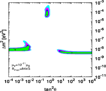
Figure 22: Allowed $\Delta m^{2}{sol}$ and $\tan^{2}\theta{sol}$ for RSFP, LMA-MSW and NRSFP solutions for the indicated values of $\mu B$, from Barranco:2002te

Note that in the presence of a neutrino transition magnetic moment of $10^{-11}$ Bohr magneton, a solar magnetic field of 80 KGauss eliminates all oscillation solutions other than LMA-MSW, irrespective of KamLAND results.

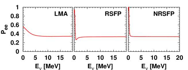
Figure 23: Best LMA-MSW and SFP $\nu_{e}$ survival probabilities from Barranco:2002te

On the other hand Fig. 23 shows the predicted solar neutrino survival probabilities for the “best” LMA-MSW solution, and for the “best” SFP solutions, from latest solar data. Clearly the spectra in the high energy region are nearly undistorted in all three cases, in agreement with observations.

Figure 24: $\Delta\chi^{2}{sol}$ versus $\tan^{2}\theta{sol}$, for RSFP, LMA-MSW (central minima) and NRSFP solutions. Left and right panels refer to two different analyses described in Ref. Barranco:2002te .

As far as the solar neutrino data are concerned, one finds that the two SFP solutions give a slightly lower $\chi^{2}{sol}$ than LMA-MSW, though all three solutions are statistically equivalent.

However, the recent first results announced by the KamLAND collaboration :2002dm imply that all non-oscillation solutions are strongly disfavored. For the case of SFP solutions one finds a rejection at about 3 $\sigma$, similar to that of non-LMA-MSW oscillation solutions before KamLAND.

7 Neutrino Decay

It is generally agreed that most probably neutrinos have non-zero masses and non-trivial mixings. This belief is based primarily on the evidence for neutrino mixings and oscillations from the solar and atmospheric neutrino data.

If neutrinos are massive they can decay. Current information on the absolute scale of neutrino mass from beta and double beta decay as well as cosmology suggests neutrino masses are at most of order of eV. Throughout the following discussion, we will stick to this assumption. In this case the only neutrino decay modes available within the simplest versions of the SM with massive neutrinos are radiative decays of the type $\nu^{\prime}\to\nu+\gamma$ and so-called invisible decays such as the three-body decay $\nu^{\prime}\to 3\nu$ Schechter:1980gr , Schechter:1981cv and two-body decays with majoron emmission seesawmajoron . The first one is ‘‘visible’’, while the latter two are ‘‘invisible’’.

The questions are (a) whether the lifetimes are short enough to be phenomenologically interesting and (b) what are the dominant decay modes. The answer to these is, unfortunately, rather model-dependent fae .

7.1 Radiative Decays

For eV neutrinos, the only radiative decay modes possible are $\nu_{i}\to\nu_{j}+\gamma$. They can occur at one–loop level in SM (Standard Model). The decay rate is given by Pal:1981rm

$$\Gamma=\frac{9}{16}\ \frac{\alpha}{\pi}\ \frac{G^{2}_{F}}{128\pi^{3}}\ \frac{\left(\delta m_{ij}^{2}\right)^{3}}{m_{i}}\left|\sum_{\alpha}\ U_{i\alpha}^{*}\ U_{\alpha j}\ \left(\frac{m_{\alpha}^{2}}{m^{2}_{W}}\right)\right|^{2}$$ (16)

where $\delta m^{2}_{ij}=m^{2}_{i}-m^{2}_{j}$ and $\alpha$ runs over $e,\mu$ and $\tau$. When $m_{i}\gg m_{j},m_{i}\sim O(eV)$ and for maximal mixing $(4U^{*2}_{i\alpha}U^{2}_{\alpha j})\sim O(1)$ and $(\alpha\cong\tau)$ one obtains for $\Gamma$

$$\Gamma_{SM}\sim 10^{-45}\ sec^{-1}$$ (17)

which is far too small to be interesting. The decay mode $\nu_{i}\to\nu_{j}+\gamma$ comes from an effective coupling which can be written as:

$$\left(\frac{e}{m_{i}+m_{j}}\right)\bar{\psi}_{j}\sigma_{\mu\nu}(C+D\gamma_{5})\psi_{i}\ F{{}_{\mu\nu}}$$ (18)

Let us define $k_{ij}$ as

$$k_{ij} = \left(\frac{e}{m_{i}+m_{j}}\right)\sqrt{\mid C\mid^{2}+\mid D\mid^{2}}\equiv k_{0}\mu_{B}$$ (19)

where $\mu_{B}=e/2m_{e}$. Since the experimental bounds on $\mu_{\nu i}$, the magnetic moments of neutrinos, come from reactions such as $\nu_{e}e\to e``\nu^{\prime\prime}$ which are not sensitive to the final state neutrinos; the bounds apply to both diagonal as well as transition magnetic moments and so can be used to limit $k^{i}_{0}$ and the corresponding lifetimes. The current bounds are pdg :

$$k^{e}_{0}\ <\ 10^{-10}$$ (20)

$$k^{\mu}_{0}\ <\ 7.4\times 10^{-10}$$

$$k^{\tau}_{0}\ <\ 5.4\times 10^{-7}$$

For $m_{i}\gg m_{j}$, the decay rate for $\nu_{i}\to\nu_{j}+\gamma$ is given by

$$\Gamma=\frac{\alpha}{2m_{e}^{2}}\ m_{i}^{3}\ k_{0}^{2}$$ (21)

This, in turn, gives indirect bounds on radiative decay lifetimes for $O(eV)$ neutrinos of:

$$\tau_{\nu_{e}}\ >\ 5\times 10^{18}\ \mbox{sec}$$ (22)

$$\tau_{\nu_{\mu}}\ >\ 5\times 10^{16}\ \mbox{sec}$$

$$\tau_{\nu_{\tau}}\ >\ 2\times 10^{11}\ \mbox{sec}$$

We realize that it is the mass eigenstates which have well defined lifetimes. Converting these bounds to ones for mass eigenstates would involve factors of mixing angles squared and with the large angles now indicated would change the above bounds by factors of 2 to 4.

There is one caveat in deducing these bounds. Namely, the form factors C and D are evaluated at $q^{2}\sim O(eV^{2})$ in the decay matrix elements whereas in the scattering from which the bounds are derived, they are evaluated at $q^{2}\sim O(MeV^{2})$. Thus, some extrapolation is necessary. It can be argued that, barring some bizarre behaviour, this is justified frere .

7.2 Invisible Neutrino Decays

7.2.1 Three-body Decays

A decay mode with essentially invisible final states which does not involve any new particles is the three-body neutrino decay mode, $\nu_{i}\to 3\nu$. In seesaw-type extensions of the standard electroweak theory these decays are mediated by the neutral-current Schechter:1981cv , due to the admixture of isosinglet and isodoublets Schechter:1980gr . As a result, in these theories there are nondiagonal couplings of the $Z$ to the mass-eigenstate neutrinos, even at the tree level Schechter:1980gr . The neutral current may be expressed in the following general form

$$P=K^{\dagger}K=\left(\begin{array}[]{ccccc}K_{L}^{\dagger}K_{L}&K_{L}^{\dagger}K_{H}\\ K_{H}^{\dagger}K_{L}&K_{H}^{\dagger}K_{H}\end{array}\right)$$ (23)

where the matrix $P=P^{2}=P^{\dagger}$ is directly determined in terms of the charged current lepton mixing matrix $K\equiv(K_{L},K_{H})$. The different entries in the $P_{LL}$ sector of the $P$ matrix determine the neutral current couplings of the light neutrinos that induce their decay. The deviation of $P_{LL}$ from the identity matrix characterizes the departure from the GIM mechanism in the neutrino sector Schechter:1980gr , Schechter:1981cv . In seesaw models this is expected to be tiny, for neutrino masses in the eV range. Although it can be enhanced in variant seesaw type models NSImodels2 , Gonzalez-Garcia:1988rw where the isosinglet heavy leptons are at the weak scale instead or possibly even lighter, this decay is still likely to be negligible.

Another way to induce this decay is through radiative corrections. Indeed, the $\nu_{i}\to 3\nu$ decay, like the radiative mode, can occur at one–loop level in SM. With a mass pattern $m_{i}\gg m_{j}$ the decay rate can be written as

$$\Gamma=\frac{\epsilon^{2}\ G^{2}_{F}\ m_{j}^{5}}{192\pi^{3}}$$ (24)

In the SM at one–loop level, with the internal $\tau$ dominating, the value of $\epsilon^{2}$ is given by Lee:1977ti

$$\epsilon_{SM}^{2}=\frac{3}{16}\left(\frac{\alpha}{\pi}\right)^{2}\left(\frac{m_{\tau}}{m_{W}}\right)^{4}\left\{\ell n\left(\frac{m_{\tau}^{2}}{m_{W}^{2}}\right)\right\}^{2}\left(U_{\tau j}\ U^{*}_{\tau i}\right)^{2}$$ (25)

With maximal mixing $\epsilon^{2}_{SM}\approx 3\times 10^{-12}$. Even if $\epsilon$ were as large as 1 with new physics contributions; it only gives a value for $\Gamma$ of $5\times 10^{-35}\ sec^{-1}$. Hence, this decay mode will not yield decay rates large enough to be of interest. Although the current experimental bound on $\epsilon$ is quite poor: $\epsilon<O(100)$, it is still strong enough to make this mode phenomenologically uninteresting, at least in vacuo.

7.2.2 Two-body Decays

There is a wide variety of models where neutrinos get masses due to the spontaneous violation of global lepton number symmetry, leading to a physical Nambu-Goldstone boson, called majoron. This leads to the most well-motivated candidate for invisible two-body neutrino decays seesawmajoron , fae

$$\nu_{\alpha_{L}}\to\nu_{\beta_{L}}+J$$ (26)

All couplings of the majoron vanish with the neutrino masses. The structure of the majoron coupling to mass-eigenstate neutrinos requires a careful diagonalization of the neutrino mass matrix Schechter:1981cv . When one performs this, typically one finds that the majoron couling matrix has a strong tendency of being diagonal. Such GIM-like effect is a generic feature of the simplest majoron schemes, first noted in Ref. Schechter:1981cv . As a result, the off-diagonal couplings of the majoron to mass eigenstate neutrinos relevant for the neutrino decays are strongly suppressed Schechter:1981cv , so that neutrino decays become irrelevant .

However, majoron couplings are rather model-dependent fae , and it is possible to contrive models where they are sizeable enough to lead to lifetimes of phenomenological interest (the first example in Ref. first-fast-decay-paper is no longer phenomenologically viable, but it is possible to arrange many variants).

An alternative way to generate fast invisible two-body neutrino decays is in models with horizontal symmetries, spontaneously broken at a scale $\left\langle\sigma\right\rangle$, instead of lepton number Gelmini:1982zz . In this case there can be several Goldstone bosons (familons), characterized by I=0, L=0, J=0. Even if there is only one familon, its coupling is typically not subject to the kind of cancellation characteristic of majoron schemes, so that the new decay mode in eq. (26) has a decay rate

$$\Gamma=\frac{g^{2}_{p}m^{3}_{\alpha}}{16\pi{\left\langle\sigma\right\rangle}^{2}}$$ (27)

characterized by a dimensionless coupling $g_{p}$ which is typically unsuppressed.

In the $SU(2)_{L}$ symmetry limit one has a similar coupling for the charged leptons, with corresponding decay modes $\ell_{\alpha}\to\ell_{\beta}+J$. Thus in this approximation the $\nu_{\alpha}$ lifetime becomes related to the B.R. $(\ell_{\alpha}\to\ell_{\beta}+J)$ through

$$\tau_{\nu_{\alpha}}=\frac{\tau_{\ell\alpha}}{B.R.(\ell_{\alpha}\to\ell_{\beta}+J)}\left(\frac{m_{\nu_{\alpha}}}{m_{\ell_{\alpha}}}\right)^{-3}$$ (28)

The current bounds on $\mu$ and $\tau$ branching ratios pdg , Jodidio:1986mz

$$B.R.(\mu\to eJ)\ <2\times 10^{-6}$$ (29)

$$B.R.(\tau\to\mu J)\ <7\times 10^{-6}$$

lead to

$$\tau_{\nu_{\mu}}>10^{24}\ \mbox{sec}$$ (30)

$$\tau_{\nu_{\tau}}>10^{20}\ \mbox{sec}.$$

These limits also hold for the case of an iso-doublet familon, $I=1/2$, $L=0$. In addition, one would need to fine tune in order to avoid mixing with the Standard Model Higgs.

However the $SU(2)_{L}$ symmetry is broken, so that the above simple argument is only a very crude approximation. The strongest direct bounds on neutrino-neutrino-Goldstone couplings is that which comes from a study of pion and kaon decays Barger:1981vd , but these bounds allow couplings strong enough that fast decays are certainly possible. Similarly the constraint Klapdor-Kleingrothaus:1999hk which comes from $\beta\beta_{0\nu}$  Berezhiani:1992cd .

From now on we simply assume that fast invisible decays of neutrinos are possible, and ask ourselves whether such decay modes can be responsible for any of the observed neutrino anomalies.

We assume a component of $\nu_{\alpha},$ i.e., $\nu_{2}$, to be the only unstable state, with a rest-frame lifetime $\tau_{0}$, and we assume two–flavor mixing, for simplicity:

$$\nu_{\alpha}=cos\theta\nu_{2}\ +sin\theta\nu_{1}$$ (31)

with $m_{2}>m_{1}$. From Eq. (2) with an unstable $\nu_{2}$, the $\nu_{\alpha}$ survival probability is

$$P_{\alpha\alpha} = sin^{4}\theta\ +cos^{4}\theta{\rm exp}(-\alpha L/E)$$

$$+ 2sin^{2}\theta cos^{2}\theta{\rm exp}(-\alpha L/2E)cos(\delta m^{2}L/2E),$$

where $\delta m^{2}=m^{2}_{2}-m_{1}^{2}$ and $\alpha=m_{2}/\tau_{0}$. Since we are attempting to explain neutrino data without oscillations there are two appropriate limits of interest. One is when the $\delta m^{2}$ is so large that the cosine term averages to 0. Then the survival probability becomes

$$P_{\mu\mu}=sin^{4}\theta\ +cos^{4}\theta{\rm exp}(-\alpha L/E)$$ (33)

Let this be called decay scenario A. The other possibility is when $\delta m^{2}$ is so small that the cosine term is 1, leading to a survival probability of

$$P_{\mu\mu}=(sin^{2}\theta+cos^{2}\theta{\rm exp}(-\alpha L/2E))^{2}$$ (34)

corresponding to decay scenario B.

The possibility of solar neutrinos decaying to explain the discrepancy is a very old suggestion Pakvasa:1972gz . The most recent analysis of the current solar neutrino data finds that no good fit can be found Bandyopadhyay:2002qg ; the conclusion is valid for both the decay scenarios A as well as B.

For atmospheric neutrinos, it was found that for the decay scenario A, it was not possible to obtain a good fit for all energies. Turning to decay scenario B, a reasonable fit was obtained for all the atmospheric data, with a minimum $\chi^{2}=33.7$ (32 d.o.f.) for the choice of parameters

$$\tau_{\nu}/m_{\nu}=63\rm~{}km/GeV,\ \cos^{2}\theta=0.30$$ (35)

The fit is of comparable quality as the one for oscillations atmdecay00 .

The reason for the similarity of the results obtained in the two models can be understood from the survival probability $P(\nu_{\mu}\to\nu_{\mu})$ of muon neutrinos as a function of $L/E_{\nu}$ for the two models using the best fit parameters is very similar. In the case of the neutrino decay model the probability $P(\nu_{\mu}\to\nu_{\mu})$ monotonically decreases from unity to an asymptotic value $\sin^{4}\theta\simeq 0.49$. In the case of oscillations the probability has a sinusoidal behaviour in $L/E_{\nu}$. The two functional forms seem very different; however, taking into account the resolution in $L/E_{\nu}$, the two forms are hardly distinguishable. In fact, in the large $L/E_{\nu}$ region, the oscillations are averaged out and the survival probability there can be well–approximated with 0.5 (for maximal mixing). In the region of small $L/E_{\nu}$ both probabilities approach unity. In the region $L/E_{\nu}$ around 400 km/GeV, where the probability for the neutrino oscillation model has the first minimum, the two curves are most easily distinguishable, at least in principle. It is entirely possible that the Super-K data and new analysis of this most recent decay model can eventually rule this out. K2K and eventually MINOS can also test this hypothesis Barger:1999bg .

Assuming that the neutrino oscillations provide the most likely explanation for the bulk of both atmospheric and solar neutrino observations; is it possible to place limits on the neutrino lifetimes? It is obvious that solar neutrino data will provide the strongest bounds currently possible. It has been argued convincingly by Beacom and Bell recently that under the most general assuptions the bound on the lifetime of $\nu_{e}$ (or the dominant mass eigenstate components thereof) is $\tau>10^{-4}$ sec for mass in the eV range Beacom:2002cb . The strongest bounds can be obtained in the future from observation of MeV neutrinos from a Galactic supernova ($\tau\sim 10^{5}\mbox{sec})$ or high energy neutrinos from AGNs ($\tau\sim 10^{3}\mbox{sec})$ decayUHE .

8 $CPT$ and Lorentz Violation

8.1 $CPT$ Violation in Neutrino Oscillations

Consequences of $CP$, $T$ and $CPT$ violation for neutrino oscillations have been written down before Schechter:1980gk , Cabibbo:1977nk . We summarize them briefly for the $\nu_{\alpha}\to\nu_{\beta}$ flavor oscillation probabilities $P_{\alpha\beta}$ at a distance $L$ from the source. If

$$P_{\alpha\beta}(L)\neq P_{\bar{\alpha}\bar{\beta}}(L)\,,\qquad\beta\neq\alpha\,,$$ (36)

then $CP$ is not conserved. If

$$P_{\alpha\beta}(L)\neq P_{\beta\alpha}(L)\,,\qquad\beta\neq\alpha\,,$$ (37)

then $T$-invariance is violated. If

$$P_{\alpha\beta}(L) \neq P_{\bar{\beta}\bar{\alpha}}(L)\,,\qquad\beta\neq\alpha\,,$$ (38)

or

$$P_{\alpha\alpha}(L) \neq P_{\bar{\alpha}\bar{\alpha}}(L)\,,$$ (39)

then $CPT$ is violated. When neutrinos propagate in matter, matter effects give rise to apparent $CP$ and $CPT$ violation even if the mass matrix is $CP$ conserving. The $CPT$ violating terms can be Lorentz-invariance violating (LV) or Lorentz invariant. The Lorentz-invariance violating, $CPT$ violating case has been discussed by Colladay and Kostelecky Colladay:1996iz and by Coleman and Glashow Coleman:1998ti .

The effective LV $CPT$ violating interaction for neutrinos is of the form

$$\bar{\nu}_{L}^{\alpha}b_{\mu}^{\alpha\beta}\gamma_{\mu}\nu_{L}^{\beta}\,,$$ (40)

where $\alpha$ and $\beta$ are flavor indices. If rotational invariance is assumed in the “preferred” frame, in which the cosmic microwave background radiation is isotropic, then the neutrino energies are eigenvalues of

$$m^{2}/2p+b_{0}\,,$$ (41)

where $b_{0}$ is a hermitian matrix, hereafter labeled $b$. In the two-flavor case the neutrino phases may be chosen such that $b$ is real, in which case the interaction in Eq. (40) is $CPT$ odd. The survival probabilities for flavors $\alpha$ and $\bar{\alpha}$ produced at $t=0$ are given by Barger:2000iv

$$P_{\alpha\alpha}(L) = 1-\sin^{2}2\Theta\sin^{2}(\Delta L/4)\,,$$ (42)

and

$$P_{\bar{\alpha}\bar{\alpha}}(L) = 1-\sin^{2}2\bar{\Theta}\sin^{2}(\bar{\Delta}L/4)\,,$$ (43)

where

$$\Delta\sin 2\Theta = \left|(\delta m^{2}/E)\sin 2\theta_{m}+2\delta be^{i\eta}\sin 2\theta_{b}\right|\,,$$ (44)

$$\Delta\cos 2\Theta = (\delta m^{2}/E)\cos 2\theta_{m}+2\delta b\cos 2\theta_{b}\,.$$ (45)

$\bar{\Delta}$ and $\bar{\Theta}$ are defined by similar equations with $\delta b\to-\delta b$. Here $\theta_{m}$ and $\theta_{b}$ define the rotation angles that diagonalize $m^{2}$ and $b$, respectively, $\delta m^{2}=m_{2}^{2}-m_{1}^{2}$ and $\delta b=b_{2}-b_{1}$, where $m_{i}^{2}$ and $b_{i}$ are the respective eigenvalues. We use the convention that $\cos 2\theta_{m}$ and $\cos 2\theta_{b}$ are positive and that $\delta m^{2}$ and $\delta b$ can have either sign. The phase $\eta$ in Eq. (44) is the difference of the phases in the unitary matrices that diagonalize $\delta m^{2}$ and $\delta b$; only one of these two phases can be absorbed by a redefinition of the neutrino states. Observable $CPT$-violation in the two-flavor case is a consequence of the interference of the $\delta m^{2}$ terms (which are $CPT$-even) and the LV terms in Eq. (40) (which are $CPT$-odd); if $\delta m^{2}=0$ or $\delta b=0$, then there is no observable $CPT$-violating effect in neutrino oscillations. If $\delta m^{2}/E\gg 2\delta b$ then $\Theta\simeq\theta_{m}$ and $\Delta\simeq\delta m^{2}/E$, whereas if $\delta m^{2}/E\ll 2\delta b$ then $\Theta\simeq\theta_{b}$ and $\Delta\simeq 2\delta b$. Hence the effective mixing angle and oscillation wavelength can vary dramatically with $E$ for appropriate values of $\delta b$. We note that a $CPT$-odd resonance for neutrinos ($\sin^{2}2\Theta=1$) occurs whenever $\cos 2\Theta=0$ or

$$(\delta m^{2}/E)\cos 2\theta_{m}+2\delta b\cos 2\theta_{b}=0\,;$$ (46)

similar to the resonance due to matter effects Wolfenstein:1977ue , Barger:2000iv . The condition for antineutrinos is the same except $\delta b$ is replaced by $-\delta b$. The resonance occurs for neutrinos if $\delta m^{2}$ and $\delta b$ have the opposite sign, and for antineutrinos if they have the same sign. A resonance can occur even when $\theta_{m}$ and $\theta_{b}$ are both small, and for all values of $\eta$; if $\theta_{m}=\theta_{b}$, a resonance can occur only if $\eta\neq 0$. If one of $\nu_{\alpha}$ or $\nu_{\beta}$ is $\nu_{e}$, then matter effects have to be included.

If $\eta=0$, then

$$\Theta = \theta\,,$$ (47)

$$\Delta = (\delta m^{2}/E)+2\delta b\,.$$ (48)

In this case a resonance is not possible. The oscillation probabilities become

$$P_{\alpha\alpha}(L) = 1-\sin^{2}2\theta\sin^{2}\left\{\left({\delta m^{2}\over 4E}+{\delta b\over 2}\right)L\right\}\,,$$ (49)

$$P_{\bar{\alpha}\bar{\alpha}}(L) = 1-\sin^{2}2\theta\sin^{2}\left\{\left({\delta m^{2}\over 4E}-{\delta b\over 2}\right)L\right\}\,.$$ (50)

For fixed $E$, the $\delta b$ terms act as a phase shift in the oscillation argument; for fixed $L$, the $\delta b$ terms act as a modification of the oscillation wavelength. An approximate direct limit on $\delta b$ when $\alpha=\mu$ can be obtained by noting that in atmospheric neutrino data the flux of downward going $\nu_{\mu}$ is not depleted, whereas that of upward going $\nu_{\mu}$ is depleted atm . Hence, the oscillation arguments in Eqs. (49) and (50) cannot have fully developed for downward neutrinos. Taking $|\delta bL/2|<\pi/2$ with $L\sim 20$ km for downward events leads to the upper bound $|\delta b|<3\times 10^{-20}$ GeV; the K2K results can improve this by an order of magnitude; upward going events could in principle test $|\delta b|$ as low as $5\times 10^{-23}$ GeV. Since the $CPT$-odd oscillation argument depends on $L$ and the ordinary oscillation argument on $L/E$, improved direct limits could be obtained by a dedicated study of the energy and zenith angle dependence of the atmospheric neutrino data.

The difference between $P_{\alpha\alpha}$ and $P_{\bar{\alpha}\bar{\alpha}}$

$$P_{\alpha\alpha}(L)-P_{\bar{\alpha}\bar{\alpha}}(L)=-2\sin^{2}2\theta\sin\left({\delta m^{2}L\over 2E}\right)\sin(\delta bL)\,,$$ (51)

can be used to test for $CPT$-violation. In a neutrino factory, the ratio of $\bar{\nu}_{\mu}\to\bar{\nu}_{\mu}$ to $\nu_{\mu}\to\nu_{\mu}$ events will differ from the Standard Model (or any local quantum field theory model) value if $CPT$ is violated. A 10kT detector, with 10¹⁹ stored muons, can probe $\delta b$ to a level of $3.10^{-23}$ GeV Bilenky:2001ka . Combining KamLAND and solar neutrino data would probe $\delta b$ to similar levels. Lorentz invariant $CPT$ violation can arise if e.g. $\delta m_{ij}^{2}$ and $\theta_{ij}$ are different for neutrinos and antineutrinos. Constraints on such differences are rather weak Barger:2000iv . Taking advantage of this, a very intriguing proposal has been made by several authors Murayama:2000hm . It was proposed that in the $\nu$ sector, the $\delta m^{2}$ and mixing are “conventional” and nearly bimaximal; namely $\delta m^{2}_{23}$ and $\delta m^{2}_{21}$ lie in the atmospheric range determined in Sec. 3.2 and in the LMA-MSW region determined in Secs. 3.1, respectively. In contrast, in the $\bar{\nu}$ sector $\delta m^{2}_{23}\sim 0(eV^{2}),\delta m^{2}_{21}$ lies in the atmospheric range and the mixing is large in the 1-2 sector but small (of order LSND) in 2-3 sector. Then the $\bar{\nu_{\mu}}-\bar{\nu}_{e}$ conversion in LSND LSND is accounted for, and the solar neutrinos are unaffected as no $\bar{\nu}^{\prime}s$ are emitted in the sun. This proposal can be tested by Mini-Boone seeing LSND effect in $\bar{\nu}_{\mu}$ beam, but not in the $\nu_{\mu}$ beam, and by the fact that the $\nu_{e}$ and $\bar{\nu}_{e}$ oscillations with $\delta m^{2}_{atm}$ will be very different (present in former and absent in latter). For example, KamLAND suzuki will see no effect in reactor $\bar{\nu}_{e}^{\prime}s$ even if LMA-MSW is the correct solution for solar $\nu_{e}^{\prime}s$. This is of course at odds with the KamLAND confirmation of the LMA-MSW solution. At neutrino factories, (fractional) $CPT$ violating mass differences and mixing parameters can be probed to a percent level Bilenky:2001ka . It should be stressed that models which have different masses for particles and anti-particles only seem Lorentz invariant (and non-local); however, the neutrino propagators will also violate Lorentz invariance and so they are actually Lorentz non-invariant as well Greenberg:2002uu .

After the announcement of KamLAND results, which are in general agreement with the expectations from LMA-MSW and hence $CPT$ conservation; a modified $CPT$-violating scenario to account for LSND has been proposed Barenboim:2002ah . The idea is that in the anti-neutrino sector, instead of the LSND and the atmospheric splittings, now there are the LSND and the KamLAND splittings. At the moment it seems possible to fit the atmospheric data. The solar mass difference and the KamLAND mass differences need not be the same, hence LMA-MSW is not yet established according to the authors.

8.2 Lorentz Invariance Violation in Neutrino Oscillations

A general formalism to describe small departures from exact Lorentz invariance has been developed by Colladay and Kostelecky Colladay:1998fq . This modification of Standard Model is renormalizable and preserves the gauge symmetries. When rotational invariance in a preferred frame is imposed, the formalism developed by Coleman and Glashow Coleman:1997xq can be used. In this form, the main effect (at high energies) of the violation of Lorentz invariance is that each particle species $i$ has its own maximum attainable velocity (MAV), $c_{i}$, in this frame. The Lorentz violating parameters are $c^{2}_{i}-c_{j}^{2}$. There are many interesting consequences Coleman:1997xq : evading of GZK cut-off, possibility of “forbidden” processes at high thresholds e.g. $\gamma\to e^{+}+e^{-},p\to e^{+}+n+\nu,\ \mu\to\pi+\nu_{\mu},\ \mu\to e+\gamma$ etc. Moreover, even if neutrinos were massless, the flavor eigenstates could be mixtures of velocity (MAV) eigenstates and the flavor survival probability (in the two flavor case) is given by

$$P_{\alpha\alpha}=1-sin^{2}2\theta\sin^{2}\left(\frac{\delta c}{2}LE\right)$$ (52)

where $\delta c=c_{1}-c_{2}$. Identical phenomenology for neutrino oscillations arises in the case of flavor violating gravity or the violation of equivalence principle (VEP), with $\delta\gamma\Phi$ replacing $\delta c$. Here $\Phi$ is the gravitational potential and $\delta\gamma=\gamma_{1}-\gamma_{2}$ is the difference in the post-Newtonian parameters used to test General Relativity Misner and which break the equivalence principle. This mechanism was first proposed by Gasperini and by Halprin and Leung Gasperini:zf , Halprin:1991gs . It provides a different realization of the phenomenon of oscillation amongst massless neutrinos, first proposed in Ref. first-NSI-resonance-paper in the context of neutrino non-standard interactions, as discussed in Sec. 5. There are, however, some important theoretical differences between the two proposals. There does not seem to be a consistent theoretical scheme for VEP, since no theory of gravity obeying the classic General Relativity tests and also violating the equivalence principle has ever been found Halprin:1995vg . In contrast the resonant oscillation of massless neutrinos due to NSI has a well-defined theoretical basis, either in terms of effective neutrino non-orthonomality, or due to the existence of new particles coupled to neutrinos first-NSI-resonance-paper , Nunokawa:1996tg . The VEP form of massless neutrino oscillations was very interesting at one time. The reason was that a single choice of parameters $\delta c$ and $\sin^{2}2\theta$ could account for both atmospheric and solar neutrinos with $\nu_{e}-\nu_{\mu}$ mixing Pantaleone:ha . However, now $\nu_{\mu}-\nu_{e}$ can no longer account for atmospheric neutrinos 3-nu-sol+atm-fit and the LE dependence is ruled out for atmospheric neutrinos learned , except as a sub-leading effect. A description of solar neutrinos, even including the recent SNO data, is still possible Raychaudhuri:2001gy ; with the choice of parameters: $\delta c/2\sim{10^{-24}}$ and large mixing. However, this is ruled out to the extent that KamLAND confirms the LMA-MSW solution for solar neutrinos; and hence must be a sub-leading effect. For $\nu_{\mu}-\nu_{x}$ mixing, the results of CCFR Naples:1998va can be used to constrain $\delta c/2<10^{-21}$ (for $sin^{2}2\theta>10^{-3})$, and future Long Baseline experiments minos will extend the bounds to $10^{-23}$ for large mixing. In the general case, when neutrinos are not massless, the energies are given by

$$E_{i}=p+m^{2}_{i}/2p+c_{i}p$$ (53)

There will be two mixing angles (even for two flavors) and the survival probability is given by

$$P_{\alpha\alpha}=1-sin^{2}2\Theta\sin^{2}(\Delta L/4)$$ (54)

where

$$\Delta\sin 2\Theta = \mid(\delta m^{2}/E)\sin 2\theta_{m}+2\delta ce^{i\eta}\ E\sin 2\theta_{c}\mid,$$ (55)

$$\Delta\cos 2\Theta = (\delta m^{2}/E)\cos 2\theta_{m}+2\delta c\ E\cos 2\theta_{c}$$ (56)

One can also write the most general expression including the $CPT$ violating term of Eq. (6) and even extending to three flavors. But there is not enough information to constraint the many new parameters. When data from Long Baseline experiments and eventually neutrino factories become available, $CPT$ and Lorentz violation in neutrino oscillations can be probed to new and significant levels. It would be especially useful to have detectors capable of distinguishing between $\nu$ and $\bar{\nu}$ events.

9 Neutrino Physics with Future Experiments

9.1 Probing Spin Flavor Precession with Borexino

Irrespective of KamLAND, future data from the upcoming Borexino experiment will be useful in distinguishing the LMA-MSW solution from the spin flavor precession solutions described above in Sec. 6. Indeed, the Borexino experiment has the potential to distinguish both the NRSFP solution and the simplest RSFP solution with no mixing Barranco:2002te , Akhmedov:2002ti from the LMA-MSW solution, as summarized in Fig. 25. See Ref. Barranco:2002te for more details.

Figure 25: Predicted $R_{\rm Borexino}$ values for LMA-MSW and spin flavor precession solutions, from Barranco:2002te

On the other hand a strong confirmation of the LMA-MSW oscillation solution by KamLAND KamLAND would imply that spin-flavor-precession may at best be present at a sub-leading level, leading to a constraint on $\mu B_{\perp}$.

Note that, if neutrino transition neutrino magnetic moments exist, then neutrino conversions within the Sun result will result in partial polarization of the initial solar neutrino fluxes. This opens a new opportunity to observe the electron antineutrinos Pastor:1997pb . By measuring the slopes of the energy dependence of the differential neutrino electron scattering cross section one can show how $\nu_{e}$ $\to$ $\bar{\nu}_{e}$ conversions may take place for low energy solar neutrinos in the Borexino region, while being unobservable at the Kamiokande and Super-Kamiokande experiments.

9.2 Probing Spin Flavor Precession with KamLAND

Accepting the LMA-MSW solution to the solar neutrino anomaly, as indicated by first KamLAND results, one can still probe the admixture of alternative mechanisms of solar neutrino conversion, such as Spin Flavor Precession. In fact we argue that this will be an interesting object of study. With sufficient statistics it should be possible to constrain such sub-leading admixtures, as discussed in Barranco:2002te . As an illustration, one can place a constraint on $\mu B_{\perp}$ (here $B_{\perp}$ is the maximum transverse solar magnetic field at the convective zone) by searching for a solar anti-neutrino flux, expected in the SFP scenarios. This constraint will depend on how good is the KamLAND determination of the LMA-MSW oscillation parameters, as illustrated in Fig. 26.

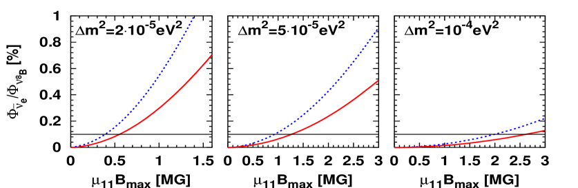
Figure 26: KamLAND sensitivity on the Majorana neutrino transition magnetic moment for the case of the LMA-MSW solution. See text.

In this Figure we have displayed the electron anti-neutrino flux predicted at KamLAND ($E>8.3$ MeV) for three different $\Delta m^{2}{sol}$ values (indicated in the figure) and for $\tan^{2}\theta{sol}$ values varying in the range from 0.3-0.8, as a function of $\mu_{11}B_{\rm max}$, $\mu_{11}$ being the magnetic moment in units of $10^{-11}$ Bohr magneton and $B_{\rm max}$ being the maximum magnetic field in the convective zone. The extremes of the neutrino mixing range correspond to the solid and dashed lines indicated in the figure, while the horizontal line corresponds to a KamLAND sensitivity on the anti-neutrino flux of 0.1 %, expected with three years running KamLAND . Clearly the limits on the transition magnetic moments are sensitive also to the ultimate central $\Delta m^{2}{sol}$ value indicated by KamLAND, being more stringent for lower $\Delta m^{2}{sol}$ values, as seen from the left panel. A 10 % error on $\Delta m^{2}{sol}$ is aimed at by the collaboration.

9.3 Constraining Neutrino Magnetic Moments with Borexino

Solar neutrino data can also be used to derive stringent bounds on Majorana neutrino transition magnetic moments $\mu_{ij}$ Schechter:1981hw , Kayser:1982br , irrespective of the value of the solar magnetic field. As discussed in Ref. Grimus:2002vb accepting that LMA-MSW accounts for the solar neutrino data, one can still probe Majorana neutrino transition magnetic moments: if present they would contribute to the neutrino–electron scattering cross section and hence affect the signal observed in Super-Kamiokande. Assuming that LMA-MSW is the solution of the solar neutrino problem Ref. Grimus:2002vb constrains neutrino TMs by using the latest global solar neutrino data. One finds that all elements of the TM matrix can be bounded at the same time. Moreover, Ref. Grimus:2002vb shown how reactor data play a complementary role to the solar neutrino data. The resulting combined solar plus reactor bound on TMs is $2\times 10^{-10}\mu_{B}$ at the 90% C.L.

Contours of the 90% C.L. bound on the magnitude of the Majorana neutrino magnetic moments after 3 years of Borexino data-taking, in units of $10^{-10}\mu_{B}$ are displayed in Fig. 27.

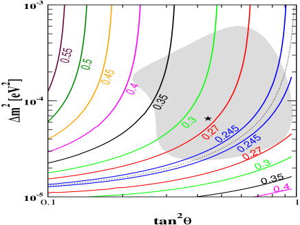
Figure 27: Contours of the 90% C.L. bound on the magnitude of the Majorana neutrino magnetic moments after 3 years of Borexino data-taking, in units of $10^{-10}\mu_{B}$. The current best fit point is shown by the star, and the shaded region is the allowed LMA-MSW region at 3$\sigma$, from first paper in Ref. Grimus:2002vb .

In this figure the current best fit point is denoted by the star, and the shaded region is the allowed 3$\sigma$ LMA-MSW region obtained in the first paper in Ref. Grimus:2002vb , where details of the analysis can be found. One sees that, thanks to the lower energy, the sensitivity of the upcoming Borexino experiment is about an order of magnitude better than that of current solar neutrino data. Given the relative delay in the start of the Borexino experiment, probing neutrino magnetic moments constitutes one of its most interesting physics goals, as no other current experiment can probe TMs with comparable sensitivity. Another interesting item for Borexino is to test for Non-Standard neutrino interactions. This possibility has been recently discussed in Ref. Berezhiani:2001rt .

9.4 Constraining New Gauge Bosons at Very Low Energies

Some electroweak models with extended neutral currents, such as those based on the $E_{6}$ group fae , lead to an increase of the $\bar{\nu}-e$ scattering cross section at low energies, typically below 100 keV Miranda:1997vs . It has been suggested in that the search for the effects of a heavy Z’ gauge boson contribution would be feasible in an experiment with a high-activity artificial neutrino source and a large-mass detector. The neutrino flux is known to within a percent accuracy and, in contrast to the reactor neutrino case, one can reach lower neutrino energies. Both features make the proposed experiment more sensitive to extended gauge models, such as the $\chi$ model fae . In Fig. 28 we briefly summarize the results obtained in Ref. Barabanov:1998bj for the case for the proposed LAMA experiment, with a large NaI(Tl) detector located at the Gran Sasso underground laboratory.

Figure 28: Attainable 95 % C. L. sensitivity to the mass (left panel) and mixing (right) of an extra gauge boson in the $\chi$ model, plotted versus the systematic error per bin. The results correspond to the cases of a 400 kg (solid line) and 1-ton detector (dashed line).

One sees that, for a low enough background, the sensitivity to the $Z_{\chi}$ boson mass would reach 600 GeV for one year running of the experiment. These values are reasonably competitive, and in any case complementary, to the sensitivity from direct searches at the Tevatron Abe:1997fd , or through precision electroweak tests precision .

9.5 Probing Non-Standard Interactions at Neutrino Factories

The primary goal of neutrino factories is to probe the lepton mixing angle $\theta_{13}$ with much better sensitivity than possible at present and, hopefully, also the possibility of leptonic $CP$ violation Apollonio:2002en , Freund:2001ui . We have already discussed both the hierarchical nature of neutrino of mass splittings indicated by the observed solar and atmospheric neutrino anomalies, as well as the stringent bound on $\theta_{13}$ that follows from reactor experiments Chooz and Palo Verde. We also mentioned in Sec. 2.1 that the leptonic $CP$ violation associated to the standard Dirac phase present in the simplest three-neutrino system (charcterized by a unitary CC mixing matrix) disappears as two neutrinos become degenerate and/or as $\theta_{13}\to 0$ Schechter:1979bn . As a result, although the large mixing indicated by current solar neutrino data certainly helps, direct leptonic $CP$ violation tests in oscillation experiments will be a very demanding task for neutrino factories.

Here we emphasise on the role of neutrino factories in probing non-standard interactions. It has been shown Huber:2001zw that NSI in the $\nu_{\mu}$ -$\nu_{\tau}$ channel can be studied with substantially improved sensitivity in the case of flavor changing NSI, especially at energies higher than approximately 50 GeV, as illustrated in Fig. 29. For example, a 100 GeV Nufact can probe FC-NSI interactions at the level of $|\epsilon|<{\rm few}\times 10^{-4}$ at 99 % C.L.

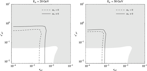
Figure 29: Comparing the sensitivity to neutrino NSI of current atmospheric neutrino experiments (white) with future neutrino factory experiments (grey), details in Ref. Huber:2001zw

Note also that in such hybrid solution to the neutrino anomalies, with FC-NSI explaining the solar data, and oscillations accounting for the atmospheric data, the two sectors are connected not only by the neutrino mixing angle $\theta_{13}$, but also by the $\nu_{e}$ -$\nu_{\tau}$ flavor changing NSI parameters. As a result NSI and oscillations may be confused, as shown in Huber:2001de . This implies that information on $\theta_{13}$ can only be obtained if bounds on NSI are available. Taking into account the existing bounds on FC interactions, one finds a drastic loss in Nufact sensitivities on $\theta_{13}$, of at least two orders of magnitude, as illustrated in Fig. 30

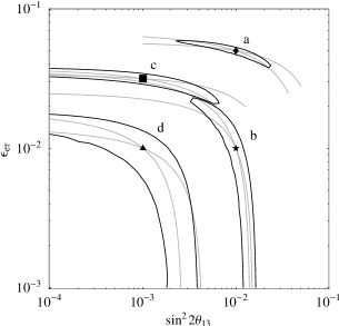
Figure 30: 99% C.L. allowed regions (black lines) in $\sin^{2}2\theta_{13}$ –$\epsilon_{e\tau}$ for different input values, as indicated by the points, at a baseline of $3\,000\,\mathrm{km}$. Lines of constant event rates are displayed in grey. Details in Ref. Huber:2001de

A near–detector offers the possibility to obtain stringent bounds on some NSI parameters and therefore constitutes a crucial necessary step towards the determination of $\theta_{13}$ and subsequent study of leptonic $CP$ violation.

10 Discussion and Outlook

These are exciting times for neutrino physics, driven mainly by experiment. We have given a brief overview on the status of neutrino oscillation physics, including the determination of mass splittings and mixings from current data. Recent results bring substantial expectation on the potential of future data both of KamLAND and K2K which provide independent tests of the solar and atmospheric neutrino anomalies from terrestrial, man-controlled neutrino sources. The solar neutrino $\Delta m^{2}{sol}$ will be better determined after 3 years of KamLAND running, especially if the solar data also improve in the meantime. Unfortunately progress in the determination of the solar angle will be less impressive. In contrast to the Cabibbo angle, the mixing between the first two generations of leptons has been shown to be large, though significantly non-maximal. This opens new ways to probe the solar interior as well as supernovae.

KamLAND has brought a turning point to the possibility of non-oscillation descriptions of the solar neutrino data, such as those invoking spin-flavor precession or non-standard neutrino interactions. Although such descriptions currently provide an excellent fit of the solar data, they are now globally disfavored by about 3 $\sigma$ and can only play a sub-leading role in the solar neutrino anomaly. Analysing in further detail the resulting constraints is beyond the scope of this short review, which was commissioned well-before these results were available.

Accepting the LMA-MSW solution, we have nevertheless illustrated how current and future neutrino data can place important restrictions on non-standard neutrino properties, such as magnetic moments. We have also discussed the potential in constraining non-standard neutrino properties of future data from experiments such as KamLAND, Borexino and the upcoming neutrino factories.

We have also considered how solar and atmospheric neutrino data can be used to place constraints on neutrino instability, as well as $CPT$ and Lorentz Violation. Let us stress that interest still persists in the investigation of non-standard neutrino properties, to the extent that, at least some, are well-motivated by theory.

Last, but not least, non-oscillation phenomena such as neutrinoless double beta decay would, if discovered, probe the absolute scale of neutrino mass and also reveal their Majorana nature. With the era of neutrino properties entering a new age, we can only hope that the underlying mechanism for generating neutrino mass will start revealing its nature, a formidable task indeed.

References

- [1] B. T. Cleveland et al., “Measurement of the Solar Electron Neutrino Flux with the Homestake Chlorine Detector,” Astrophys. J. 496, 505 (1998).
- [2] W. Hampel et al. [GALLEX Collaboration], “GALLEX solar neutrino observations:…,” Phys. Lett. B 447, 127 (1999).
- [3] J. N. Abdurashitov et al. [SAGE Collaboration], “Measurement of the solar neutrino capture rate by SAGE…,” Phys. Rev. Lett. 83, 4686 (1999); Phys. Rev. C 60, 055801 (1999); J. Exp. Theor. Phys. 95, 181 (2002) [Zh. Eksp. Teor. Fiz. 122, 211 (2002)]
- [4] M. Altmann et al. [GNO Collaboration], “GNO solar neutrino observations…,” Phys. Lett. B 490, 16 (2000); E. Bellotti, Nucl. Phys. Proc. Suppl. 91, 44 (2001).
- [5] S. Fukuda et al. [Super-K Collaboration], “Determination of solar neutrino oscillation parameters using 1496 days…,” Phys. Lett. B 539, 179 (2002) and references therein
- [6] Q. R. Ahmad et al. [SNO Collaboration], “Direct evidence for neutrino flavor transformation from neutral-current …; Phys. Rev. Lett. 89, 011301 (2002), and “Measurement of day and night neutrino energy spectra at SNO…” Phys. Rev. Lett. 89, 011302 (2002)
- [7] Q. R. Ahmad et al. [SNO Collaboration], “Measurement of the charged current interactions produced by B-8 solar neutrinos…,” Phys. Rev. Lett. 87, 071301 (2001)
- [8] J. Bahcall, Int. Conf. on Neutrino Physics and Astrophysics, Munich 2002; B. Ricci, V. Berezinsky, S. Degl’Innocenti, W. A. Dziembowski, G. Fiorentini, “Helioseismic constraints to the central solar temperature and neutrino fluxes,” Phys. Lett. B 407 (1997) 155
- [9] M. Maltoni, T. Schwetz, M. A. Tortola and J. W. Valle, “Constraining neutrino oscillation parameters with current solar and atmospheric data,” Phys. Rev. D 67 013011 (2003), [arXiv:hep-ph/0207227]. This paper gives an extensive list of earlier references on solar neutrino data analyses
- [10] L. Wolfenstein, “Neutrino Oscillations In Matter,” Phys. Rev. D 17, 2369 (1978); S. P. Mikheev and A. Y. Smirnov, “Resonance Enhancement of Oscillations…,” Sov. J. Nucl. Phys. 42 (1985) 913
- [11] M. C. Gonzalez-Garcia et al, “Status of the MSW solutions of the solar neutrino problem,” Nucl. Phys. B 573, 3 (2000); J. N. Bahcall, P. I. Krastev, A. Y. Smirnov, Phys. Rev. D 60 (1999) 093000
-
[12]
Y. Fukuda et al.,
Kamiokande Coll., Phys. Lett. B 335 (1994) 237;
R. Becker-Szendy et al.,
IMB Coll., Nucl. Phys. B (Proc. Suppl.) 38 (1995) 331;
W.W.M. Allison et al., Soudan Coll.,
Phys. Lett. B 449 (1999) 137.
Super-Kamiokande Coll., Y. Fukuda et al., Phys. Rev. Lett.
81 (1998) 1562 and 82 (1999) 2644; C. McGrew in
Neutrino Telescopes 2001, Venice, Italy, March 2001; T.
Toshito in Moriond 2001, Les Arcs, France, March 2001.
MACRO Coll., M. Ambrosio et al., Phys. Lett. B 434
(1998) 451; M. Spurio et al., hep-ex/0101019; B. Barish, Proc.
of Neutrino 2000,
http://nu2000.sno.laurentian.ca}. A. Surdo, Talk given at TAUP 2001, 8–12 September 2001, Gran Sasso, Italy (http://www.lngs.infn.it/). - [13] G. Battistoni et al “Progresses in the validation of the FLUKA atmospheric nu flux calculations,” Nucl. Phys. Proc. Suppl. 110 (2002) 336
- [14] A. Aguilar et al. [LSND Collaboration], “Evidence for neutrino oscillations…” Phys. Rev. D 64, 112007 (2001) See also talk by G. Drexlin, at International Conference on Neutrino Physics and Astrophysics, http://neutrino2002.ph.tum.de/pages/transparencies2.html
- [15] Y. Declais et al., “Search for neutrino oscillations… from a nuclear power reactor at Bugey,” Nucl. Phys. B 434 (1995) 503.
- [16] F. Dydak et al., “A Search For Muon-Neutrino Oscillations…,” Phys. Lett. B 134 (1984) 281.
- [17] B. Armbruster et al. [KARMEN Collaboration], “Upper limits for neutrino oscillations ….,” Phys. Rev. D 65 (2002) 112001
- [18] M. Apollonio et al. [CHOOZ Collaboration], “Limits on neutrino oscillations from the CHOOZ experiment,” Phys. Lett. B 466 (1999) 415; F. Boehm et al, [Palo Verde Coll], “Final results from the Palo Verde…,” Phys. Rev. D 64 (2001) 112001
- [19] K. Eguchi et al [KamLAND Collaboration], “First results from KamLAND: Evidence for reactor anti-neutrino disappearance,” hep-ex/0212021.
- [20] M. H. Ahn et al. [K2K Collaboration], “Indications of neutrino oscillation in a 250-km long-baseline experiment,” hep-ex/0212007.
- [21] M. Gell-Mann, P. Ramond and R. Slansky in Supergravity (North Holland, Amsterdam 1979); T. Yanagida in Proc. of the Workshop on Unified Theory and Baryon Number of the Universe, KEK, Japan, 1979.
- [22] R. N. Mohapatra and G. Senjanovic, “Neutrino Mass And Spontaneous Parity Nonconservation,” Phys. Rev. Lett. 44 (1980) 912; J. Schechter and J. W. F. Valle, “Neutrino Masses in SU(2) U(1) Theories,” Phys. Rev. D 22, 2227 (1980)
- [23] Y. Chikashige, R. N. Mohapatra and R. D. Peccei, “Are there Real Goldstone Bosons …?,” Phys. Lett. B 98 (1981) 265; J. Schechter and J. W. F. Valle, “Neutrino Decay And Spontaneous Violation Of Lepton Number,” Phys. Rev. D 25 (1982) 774; G. B. Gelmini and J. W. F. Valle, “Fast Invisible Neutrino Decays,” Phys. Lett. B 142, 181 (1984).
- [24] S. Weinberg, “Opening Address, Neutrinos 78” Proc., West Lafayette 1978, 1; R. Barbieri, J. R. Ellis and M. K. Gaillard, “Neutrino Masses and Oscillations in SU(5),” Phys. Lett. B 90, 249 (1980).
- [25] A. Zee, “A Theory Of Lepton Number Violation…,” Phys. Lett. B 93 (1980) 389 [Err-ibid. B 95 (1980) 461]; K. S. Babu, “Model Of ’Calculable’…,” Phys. Lett. B 203 (1988) 132.
- [26] A. Masiero and J. W. Valle, “A Model For Spontaneous R Parity Breaking,” Phys. Lett. B 251 (1990) 273; J. C. Romao et al, “How To Spontaneously Break R-Parity,” Phys. Lett. B 288 (1992) 311; J. C. Romao and J. W. Valle, “Neutrino Masses In Supersymmetry…,” Nucl. Phys. B 381 (1992) 87. For early, pre-LEP papers, see C. S. Aulakh, R. N. Mohapatra, Phys. Lett. B 119 (1982) 13; G. G. Ross, J. W. F. Valle, Phys. Lett. B 151 (1985) 375; J. R. Ellis et al, Phys. Lett. B 150 (1985) 142; A. Santamaria, J. W. F. Valle, Phys. Lett. B 195, 423 (1987); Phys. Rev. Lett. 60, 397 (1988); Phys. Rev. D 39, 1780 (1989).
- [27] M. A. Diaz et al, “Minimal supergravity with R-parity breaking,” Nucl. Phys. B 524 (1998) 23; M. Hirsch et al, “Neutrino masses and mixings from supersymmetry…” Phys. Rev. D 62 (2000) 113008 [Err-ibid. D 65 (2002) 119901] and references therein.
- [28] M. Hirsch et al, “Probing neutrino properties with charged scalar lepton decays,” Phys. Rev. D 66 (2002) 095006; W. Porod et al, “Testing neutrino mixing at future collider experiments,” Phys. Rev. D 63 (2001) 115004; D. Restrepo, W. Porod and J. W. Valle, “Broken R-parity, stop decays, and neutrino physics,” Phys. Rev. D 64 (2001) 055011; S. Y. Choi, E. J. Chun, S. K. Kang and J. S. Lee, “Neutrino oscillations and R-parity… signals,” Phys. Rev. D 60 (1999) 075002; J. C. Romao et al, “A supersymmetric solution…,” Phys. Rev. D 61, 071703 (2000) B. Mukhopadhyaya, S. Roy and F. Vissani, “Correlation between neutrino oscillations…,” Phys. Lett. B 443 (1998) 191
- [29] A. Ioannisian and J. W. Valle, “SO(10) grand unification model for degenerate neutrino masses,” Phys. Lett. B 332 (1994) 93; D. O. Caldwell and R. N. Mohapatra, “Neutrino Mass Explanations Of Solar And Atmospheric Neutrino Deficits And Hot Dark Matter,” Phys. Rev. D 48 (1993) 325
- [30] K. S. Babu, E. Ma and J. W. F. Valle, “Underlying A(4) symmetry for the neutrino mass matrix and the quark mixing matrix,” Phys. Lett. B 552 (2003) 207 [hep-ph/0206292]
- [31] See, e. g. P. H. Chankowski et al, “Neutrino unification,” Phys. Rev. Lett. 86 (2001) 3488 [hep-ph/0011150]
- [32] S. Davidson and S. F. King, “Bi-maximal neutrino mixing in the MSSM with a single right-handed neutrino,” Phys. Lett. B 445 (1998) 191; Q. Shafi and Z. Tavartkiladze, “Bi-maximal neutrino mixings and proton decay in SO(10)…,” Phys. Lett. B 487 (2000) 145 K. S. Babu and R. N. Mohapatra, “Predictive schemes for bimaximal neutrino mixings,” Phys. Lett. B 532 (2002) 77.
- [33] For reviews see, e. g. G. Altarelli and F. Feruglio, “Neutrino Masses And Mixings: A Theoretical Perspective,” Phys. Rept. 320 (1999) 29; S. M. Barr and I. Dorsner, “A general classification of three neutrino models…,” Nucl. Phys. B 585 (2000) 79; G. G. Ross and L. Velasco-Sevilla, “Symmetries and fermion masses,” hep-ph/0208218, and S. King talk at Neutrino 2002.
- [34] J. Schechter and J. W. F. Valle, “Neutrino Masses in SU(2) U(1) Theories,” Phys. Rev. D 22 (1980) 2227.
- [35] J. Schechter and J. W. F. Valle, “Neutrino Oscillation Thought Experiment,” Phys. Rev. D 23 (1981) 1666.
- [36] M. Doi, T. Kotani, H. Nishiura, K. Okuda and E. Takasugi, “CP Violation in Majorana Neutrinos,” Phys. Lett. B 102 (1981) 323. For a recent review see S. M. Bilenky, C. Giunti and W. Grimus, “Phenomenology of neutrino oscillations,” Prog. Part. Nucl. Phys. 43 (1999) 10
- [37] J. Schechter, J. W. F. Valle, “Comment on The Lepton Mixing Matrix” Phys. Rev. D 21 (1980) 309
- [38] G. C. Branco et al, “Leptonic CP Violation with Massless Neutrinos,” Phys. Lett. B 225 (1989) 385; N. Rius, J. W. F. Valle, “Leptonic CP Violating Asymmetries…,” Phys. Lett. B 246 (1990) 249; M. C. Gonzalez-Garcia and J. W. F. Valle, “Enhanced lepton flavor violation with massless neutrinos…,” Mod. Phys. Lett. A 7 (1992) 477; A. Ilakovac, A. Pilaftsis, Nucl. Phys. B 437 (1995) 491; J. Bernabeu et al, Phys. Lett. B 187 (1987) 303.
- [39] For a review see J. W. F. Valle, “Gauge Theories And The Physics of Neutrino Mass,” Prog. Part. Nucl. Phys. 26, 91 (1991).
- [40] R. N. Mohapatra and J. W. F. Valle, “Neutrino Mass And Baryon-Number Nonconservation In Superstring Models,” Phys. Rev. D 34 (1986) 1642.
- [41] J. W. F. Valle, “Resonant Oscillations of Massless Neutrinos In Matter,” Phys. Lett. B 199, 432 (1987).
- [42] J. T. Peltoniemi, D. Tommasini and J. W. F. Valle, “Reconciling dark matter and solar neutrinos,” Phys. Lett. B 298, 383 (1993); J. T. Peltoniemi and J. W. F. Valle, “Reconciling dark matter, solar and atmospheric neutrinos,” Nucl. Phys. B 406, 409 (1993); Caldwell & Mohapatra in Ioannisian:1994nx Giunti and Lavader’s excellent web–page http://www.to.infn.it/ giunti/neutrino/
- [43] M. Maltoni, T. Schwetz and J. W. F. Valle, “Status of four-neutrino mass schemes: A global and unified approach to current neutrino oscillation data,” Phys. Rev. D 65, 093004 (2002) [hep-ph 0112103]
- [44] M. Maltoni, T. Schwetz, M. A. Tortola and J. W. F. Valle, “Ruling out four-neutrino oscillation interpretations of the LSND anomaly?,” Nucl. Phys. B 643 (2002) 321 [hep-ph/0207157]
- [45] A. Osipowicz et al. [KATRIN Coll], “Katrin: A next generation tritium beta decay experiment with sub-eV sensitivity for the electron neutrino mass,” hep-ex/0109033 and references therein
- [46] O. Elgaroy et al, “A new limit on the total neutrino mass from the 2dF galaxy redshift survey,” astro-ph/0204152. For a theoretical discussion see S. Hannestad, astro-ph/0211106.
- [47] K. Hagiwara et al. “Review Of Particle Physics,” Phys. Rev. D 66 (2002) 010001
- [48] For reviews on double beta decay experiments and nuclear theory see, A. Morales, Nucl. Phys. Proc. Suppl. 77, 335 (1999); P. Vogel, nucl-th/0005020; A. Faessler and F. Simkovic, Prog. Part. Nucl. Phys. 46 (2001) 233; M. Doi, T. Kotani and E. Takasugi, “Double Beta Decay And Majorana Neutrino,” Prog. Theor. Phys. Suppl. 83, 1 (1985).
- [49] J. Schechter and J. W. F. Valle, “Neutrinoless Double-Beta Decay In SU(2) X U(1) Theories,” Phys. Rev. D 25, 2951 (1982).
- [50] L. Wolfenstein, “Different Varieties Of Massive Dirac Neutrinos,” Nucl. Phys. B 186 (1981) 147; J. W. F. Valle and M. Singer, “Lepton Number Violation with Quasi Dirac Neutrinos,” Phys. Rev. D 28, 540 (1983).
- [51] J. W. F. Valle, “Neutrinoless Double-Beta Decay with Quasi-Dirac Neutrinos,” Phys. Rev. D 27, 1672 (1983).
- [52] V. Barger, S. L. Glashow, D. Marfatia, K. Whisnant, “Neutrinoless double beta decay can constrain neutrino dark matter,” Phys. Lett. B 532 (2002) 15; F. Feruglio, A. Strumia, F. Vissani, “Neutrino oscillations and signals in beta and 0nu 2beta experiments,” Nucl. Phys. B 637 (2002) 345; H. Minakata, H. Sugiyama, “Constraints on neutrino mixing parameters by observation of neutrinoless double beta decay,” Phys. Lett. B 532, 275 (2002)
- [53] H. V. Klapdor-Kleingrothaus et al. [GENIUS Collaboration], “GENIUS: A supersensitive germanium detector system for rare events,” hep-ph/9910205; E. Fiorini, “Cuore: A Cryogenic Underground Observatory For Rare Events,” Phys. Rept. 307, 309 (1998); A. Bettini, “Neutrino Physics At Gran Sasso Laboratory,” Nucl. Phys. Proc. Suppl. 100, 332 (2001).
- [54] M. C. Gonzalez-Garcia et al, “Global three-neutrino oscillation analysis of neutrino data,” Phys. Rev. D 63, 033005 (2001) [hep-ph/0009350].
- [55] Talk by E. Lisi at XXth International Conference on Neutrino Physics and Astrophysics, http://neutrino2002.ph.tum.de/pages/transparencies2.html and references therein
- [56] J. Barranco et al, “Confronting spin flavor solutions of the solar neutrino problem with current and future solar neutrino data,” Phys. Rev. D 66 (2002) 093009 [hep-ph/0207326].
- [57] N. Fornengo et al, “Probing neutrino non-standard interactions with atmospheric neutrino data,” Phys. Rev. D 65, 013010 (2002) [hep-ph/0108043].
- [58] N. Fornengo et al, “Updated global analysis of the atmospheric neutrino data in terms of neutrino oscillations,” Nucl. Phys. B 580, 58 (2000) [hep-ph/0002147].
- [59] M. Maltoni, T. Schwetz and J. W. F. Valle, “Combining first KamLAND results with solar neutrino data,” hep-ph/0212129.
- [60] P. Vogel and J. Engel, “Neutrino Electromagnetic Form-Factors,” Phys. Rev. D 39, 3378 (1989).
- [61] H. Murayama and A. Pierce, “Energy spectra of reactor neutrinos at KamLAND,” Phys. Rev. D 65, 013012 (2002)
- [62] The KamLAND proposal, Stanford-HEP-98-03; A. Piepke, talk at Neutrino-2000, XIXth International Conference on Neutrino Physics and Astrophysics, Sudbury, Canada, June 2000.
- [63] P. Vogel and J. F. Beacom, “The angular distribution of the reaction + p ,” Phys. Rev. D 60, 053003 (1999)
- [64] E. D. Church, K. Eitel, G. B. Mills and M. Steidl, “Statistical analysis of different searches,” Phys. Rev. D 66 (2002) 013001
- [65] P. C. de Holanda, A. Smirnov, hep-ph/0212270; P. Aliani et al, hep-ph/0212212; H. Nunokawa, W. J. Teves, R. Z. Funchal, hep-ph/0212202; J. N. Bahcall, M. C. Gonzalez-Garcia, C. Pena-Garay, hep-ph/0212147; A. Bandyopadhyay, S. Choubey, R. Gandhi, S. Goswami, D. P. Roy, hep-ph/0212146; G. L. Fogli, E. Lisi, A. Marrone, D. Montanino, A. Palazzo, A. M. Rotunno, hep-ph/0212127; V. Barger, D. Marfatia, hep-ph/0212126; H. Minakata, H. Sugiyama, hep-ph/0212240.
- [66] A. de Gouvea and C. Pena-Garay, “Solving the solar neutrino…,” Phys. Rev. D 64, 113011 (2001)
- [67] V. D. Barger, D. Marfatia and B. P. Wood, “Resolving the solar neutrino problem with KamLAND,” Phys. Lett. B 498, 53 (2001)
- [68] A. D. Dolgov, “Neutrinos in cosmology,” Phys. Rept. 370, 333 (2002); G. G. Raffelt, “Astrophysical and cosmological neutrinos,” hep-ph/0208024. These papers give extensive references
- [69] A. D. Dolgov, S. H. Hansen, S. Pastor, S. T. Petcov, G. G. Raffelt and D. V. Semikoz, “Cosmological bounds on neutrino degeneracy improved by flavor oscillations,” Nucl. Phys. B 632 (2002) 363
- [70] E. Lisi, S. Sarkar and F. L. Villante, “The big bang nucleosynthesis limit on ” Phys. Rev. D 59 (1999) 123520
- [71] C. Burgess et al, “Large mixing angle oscillations as a probe of the deep solar interior,” hep-ph/0209094; H. Nunokawa et al, “The effect of random matter density perturbations…,” Nucl. Phys. B 472, 495 (1996); A. B. Balantekin, J. M. Fetter and F. N. Loreti, “The MSW effect in a fluctuating matter density,” Phys. Rev. D 54, 3941 (1996); P. Bamert, C. P. Burgess and D. Michaud, “Neutrino propagation through helioseismic waves,” Nucl. Phys. B 513, 319 (1998)
- [72] M. T. Keil, G. G. Raffelt and H. T. Janka, “Monte Carlo study of supernova neutrino spectra formation,” astro-ph/0208035.
- [73] A. Y. Smirnov, D. N. Spergel, J. N. Bahcall, “Is Large Lepton Mixing Excluded?,” Phys. Rev. D 49, 1389 (1994); B. Jegerlehner, F. Neubig, G. Raffelt, Phys. Rev. D 54, 1194 (1996); M. Kachelriess, R. Tomas, J. W. F. Valle, “Large lepton mixing and supernova 1987A,” JHEP 0101, 030 (2001)
- [74] M. Kachelriess et al, “SN1987A and the status of oscillation solutions to the solar neutrino problem,” Phys. Rev. D 65, 073016 (2002) [hep-ph/0108100].
- [75] H. Minakata et al, “Probing supernova physics with neutrino oscillations,” Phys. Lett. B 542, 239 (2002) [hep-ph/0112160].
- [76] G.G. Raffelt, private communication
- [77] H. Nunokawa et al, “Resonant conversion of massless neutrinos in supernovae,” Phys. Rev. D 54, 4356 (1996); H. Nunokawa et al, “Supernova bounds on supersymmetric R-parity violating interactions,” Nucl. Phys. B 482, 481 (1996); D. Grasso et al, “Pulsar velocities without neutrino mass,” Phys. Rev. Lett. 81, 2412 (1998).
- [78] G. L. Fogli, E. Lisi, A. Mirizzi and D. Montanino, “Revisiting nonstandard interaction effects on supernova neutrino flavor oscillations,” Phys. Rev. D 66 (2002) 013009 and papers therein
- [79] M. Kachelriess, R. Tomas and J. W. F. Valle, “Supernova bounds on majoron-emitting decays of light neutrinos,” Phys. Rev. D 62 (2000) 023004 [hep-ph/0001039]. See also Y. Farzan, “Bounds on the coupling of the majoron to light neutrinos from supernova cooling,” hep-ph/0211375.
- [80] L. J. Hall and M. Suzuki, “Explicit R Parity Breaking In Supersymmetric Models,” Nucl. Phys. B 231 (1984) 419; For a recent review see B. Allanach et al, “Searching for R-parity violation at Run-II of the Tevatron,” hep-ph/9906224
- [81] L. J. Hall, V. A. Kostelecky and S. Raby, “New Flavor Violations In Supergravity Models,” Nucl. Phys. B 267 (1986) 415. R. Barbieri, L. J. Hall and A. Strumia, “Violations of lepton flavor and CP…,” Nucl. Phys. B 445, 219 (1995); F. Gabbiani, E. Gabrielli, A. Masiero and L. Silvestrini, “A complete analysis of FCNC and CP…,” Nucl. Phys. B 477 (1996) 321
- [82] M. Guzzo et al, “Status of a hybrid three-neutrino interpretation of neutrino data,” Nucl. Phys. B 629, 479 (2002) [hep-ph/0112310]. For early Refs. see Wolfenstein:1977ue , first-NSI-resonance-paper , and also M. M. Guzzo, A. Masiero and S. T. Petcov, “On the MSW effect with massless…,” Phys. Lett. B 260 (1991) 15, and E. Roulet, “Mikheyev-Smirnov-Wolfenstein effect with flavor-changing…,” Phys. Rev. D 44 (1991) 935.
- [83] M. C. Gonzalez-Garcia et al, “Atmospheric neutrino observations and flavor changing interactions,” Phys. Rev. Lett. 82, 3202 (1999); N. Fornengo et al, JHEP 0007, 006 (2000)
- [84] K. Fujikawa and R. Shrock, “The Magnetic Moment Of A Massive Neutrino And Neutrino Spin Rotation,” Phys. Rev. Lett. 45 (1980) 963.
- [85] A.I. Derbin et al., “Experiment On Anti-Neutrino Scattering by Electrons…” JETP Lett. 57 (1993) 768 [Pisma Zh. Eksp. Teor. Fiz. 57 (1993) 755]. A.V. Derbin, “Restriction On The Magnetic Dipole Moment Of Reactor Neutrinos,” Phys. Atom. Nucl. 57 (1994) 222 [Yad. Fiz. 57 (1994) 236].
- [86] H. B. Li [Texono Collaboration], “New limits on neutrino magnetic moments…,” hep-ex/0212003.
-
[87]
C. Broggini, MUNU Collaboration,
“Preliminary Results And Status Of The Munu Experiment,”
Nucl. Phys. (Proc. Suppl.) 100 (2001) 267;
J. Vuilleumier, Talk at Neutrino 2002, Munich,
http://neutrino2002.ph.tum.de/. - [88] L. B. Auerbach et al. [LSND Collaboration], “Measurement of electron elastic scattering,” Phys. Rev. D 63 (2001) 112001
- [89] R. Schwienhorst et al. [DONUT Collaboration], “A new upper limit for the tau-neutrino magnetic moment,” Phys. Lett. B 513 (2001) 23
- [90] G.G. Raffelt, “Limits On Neutrino Electromagnetic Properties: An Update,” Phys. Rept. 320 (1999) 319.
- [91] B. S. Neganov et al, “Status of the experiment on the laboratory search for the electron antineutrino magnetic moment…,” Phys. Atom. Nucl. 64 (2001) 1948 [Yad. Fiz. 64 (2001) 2033]
- [92] J. Schechter and J. W. F. Valle, “Majorana Neutrinos And Magnetic Fields,” Phys. Rev. D 24, 1883 (1981) [Err.-ibid. D 25, 283 (1982)].
- [93] A. Cisneros, “Effect Of Neutrino Magnetic Moment On Solar Neutrino Observations,” Astrophys. Space Sci. 10 (1971) 87; L. B. Okun, M. B. Voloshin and M. I. Vysotsky, “Electromagnetic Properties Of Neutrino And Possible Semiannual Variation Of The Solar Neutrino Flux,” Sov. J. Nucl. Phys. 44 (1986) 440
- [94] G. Raffelt, “Stars as Laboratories for Fundamental Physics”, University of Chicago Press (1996)
- [95] E. K. Akhmedov, “Resonant Amplification Of Neutrino Spin Rotation In Matter And The Solar-Neutrino Problem,” Phys. Lett. B 213 (1988) 64. C. S. Lim and W. J. Marciano, “Resonant Spin-Flavor Precession Of Solar And Supernova Neutrinos,” Phys. Rev. D 37 (1988) 1368.
- [96] O. G. Miranda et al, “The simplest resonant spin-flavour solution to the solar neutrino problem,” Nucl. Phys. B 595, 360 (2001)
- [97] O. G. Miranda et al, “A non-resonant dark-side solution to the solar neutrino problem,” Phys. Lett. B 521, 299 (2001) [hep-ph/0108145].
- [98] J. Schechter and J. W. F. Valle, “Neutrino Decay And Spontaneous Violation Of Lepton Number,” Phys. Rev. D 25 (1982) 774.
- [99] P. B. Pal and L. Wolfenstein, “Radiative Decays Of Massive Neutrinos,” Phys. Rev. D 25 (1982) 766; S. Petcov, Sov. J. of Nucl. Phys. 24, 340 (1977); W. Marciano and A. Sanda, Phys. Lett. B67, 303 (1977).
- [100] J. M. Frere, R. B. Nevzorov and M. I. Vysotsky, “Stimulated neutrino conversion and bounds on neutrino magnetic moments,” Phys. Lett. B 394 (1997) 127
- [101] M. C. Gonzalez-Garcia and J. W. F. Valle, “Fast Decaying Neutrinos And Observable Flavor Violation In A New Class Of Majoron Models,” Phys. Lett. B 216 (1989) 360.
- [102] B. W. Lee and R. E. Shrock, “Natural Suppression Of Symmetry Violation In Gauge Theories: Muon - Lepton And Electron Lepton Number Nonconservation,” Phys. Rev. D 16 (1977) 1444.
- [103] A. D. Dolgov et al, “Primordial nucleosynthesis, majorons…,” Nucl. Phys. B 496 (1997) 24 [hep-ph/9610507].
- [104] J. W. F. Valle, “Fast Neutrino Decay In Horizontal Majoron Models,” Phys. Lett. B 131 (1983) 87.
- [105] G. B. Gelmini, S. Nussinov and T. Yanagida, “Does Nature Like Nambu-Goldstone Bosons?,” Nucl. Phys. B 219 (1983) 31.
- [106] A. Jodidio et al., “Search For Right-Handed Currents In Muon Decay,” Phys. Rev. D 34 (1986) 1967 [Err-ibid. D 37 (1988) 237].
- [107] V. D. Barger, W. Y. Keung and S. Pakvasa, “Majoron Emission By Neutrinos,” Phys. Rev. D 25 (1982) 907.
- [108] Z. G. Berezhiani et al, “Observable Majoron emission in neutrinoless double beta decay,” Phys. Lett. B 291 (1992) 99 [hep-ph/9207209].
- [109] S. Pakvasa and K. Tennakone, “Neutrinos Of Non-Zero Rest Mass,” Phys. Rev. Lett. 28 (1972) 1415; J. N. Bahcall, N. Cabibbo and A. Yahil, “Are Neutrinos Stable Particles?,” Phys. Rev. Lett. 28 (1972) 316; J. N. Bahcall et al, “Tests Of Neutrino Stability,” Phys. Lett. B 181 (1986) 369.
- [110] A. Bandyopadhyay, S. Choubey and S. Goswami, “Neutrino decay confronts the SNO data,” hep-ph/0204173; A. S. Joshipura, E. Masso and S. Mohanty, “Constraints on decay plus oscillation solutions…,” Phys. Rev. D 66 (2002) 113008
- [111] P. Lipari and M. Lusignoli, Phys. Rev. D60, 013003 (1999); G. Fogli et al., Phys. Rev. D59, 117303(1999); S. Choubey and S. Goswami, Astropart. Phys. 14, 67(2000).
- [112] V. D. Barger, J. G. Learned, P. Lipari, M. Lusignoli, S. Pakvasa and T. J. Weiler, “Neutrino decay and atmospheric neutrinos,” Phys. Lett. B 462 (1999) 109
- [113] J. F. Beacom and N. F. Bell, “Do solar neutrinos decay?,” Phys. Rev. D 65 (2002) 113009
- [114] J. F. Beacom, N. F. Bell, D. Hooper, S. Pakvasa and T. J. Weiler, “Decay of high-energy astrophysical neutrinos,” hep-ph/0211305.
- [115] N. Cabibbo, Phys. Lett. B 72, 333 (1978). S. Pakvasa, Proc. of the XXth Int. Conference on High Energy Physics, ed. by L. Durand and L.G.Pondrom, AIP Conf. Proc. No. 68 (New York, 1981), Vol. 2, p. 1164; V. Barger, K. Whisnant and R.N. Phillips, Phys. Rev. Lett. 45, 2084 (1980).
- [116] D. Colladay and V. A. Kostelecky, “CPT violation and the standard model,” Phys. Rev. D 55, 6760 (1997)
- [117] S. R. Coleman and S. L. Glashow, “High-energy tests of Lorentz invariance,” Phys. Rev. D 59, 116008 (1999)
- [118] V. D. Barger, S. Pakvasa, T. J. Weiler and K. Whisnant, “CPT odd resonances in neutrino oscillations,” Phys. Rev. Lett. 85, 5055 (2000)
- [119] S. M. Bilenky, M. Freund, M. Lindner, T. Ohlsson and W. Winter, “Tests of CPT invariance at neutrino factories,” Phys. Rev. D 65 (2002) 073024
- [120] H. Murayama and T. Yanagida, “LSND, SN1987A, and CPT violation,” Phys. Lett. B 520 (2001) 263; G. Barenboim, L. Borissov, J. Lykken and A. Y. Smirnov, “Neutrinos as the messengers of CPT violation,” JHEP 0210 (2002) 001
- [121] A. Suzuki, 8th International Workshop on Neutrino Telescopes, Venice, Feb. 23-26, 1999, Ed. M. Baldo-Ceolin, Vol. I. p. 325.
- [122] O. W. Greenberg, “CPT violation implies violation of Lorentz invariance,” Phys. Rev. Lett. 89, 231602 (2002)
- [123] G. Baremboim, L. Borissov and J. Lykken, “CPT violating neutrinos in the light of KamLAND,” hep-ph/0212116.
- [124] D. Colladay and V. A. Kostelecky, “Lorentz-violating extension of the standard model,” Phys. Rev. D 58 (1998) 116002
- [125] S. R. Coleman and S. L. Glashow, “Cosmic ray and neutrino tests of special relativity,” Phys. Lett. B 405 (1997) 249 [hep-ph/9703240].
- [126] See, e. g. C. W. Misner, K. S. Thorne, and J. A. Wheeler. “Gravitation”. W. H. Freeman, San Francisco, 1973; or S. Weinberg, “Gravitation and Cosmology: Principles and Applications of the General Theory of Relativity”, John Wiley & Sons, ISBN: 0471925675
- [127] M. Gasperini, “Testing The Principle Of Equivalence With Neutrino Oscillations,” Phys. Rev. D 38, 2635 (1988).
- [128] A. Halprin and C. N. Leung, “Can the sun shed light on neutrino gravitational interactions?,” Phys. Rev. Lett. 67, 1833 (1991).
- [129] A. Halprin, C. N. Leung and J. Pantaleone, “A Possible Violation of the Equivalence Principle by Neutrinos,” Phys. Rev. D 53, 5365 (1996)
- [130] J. Pantaleone, A. Halprin, C. N. Leung, “Neutrino Mixing Due to a Violation of the Equivalence Principle,” Phys. Rev. D 47 (1993) 4199; J. N. Bahcall, P. I. Krastev, C. N. Leung, “Solar neutrinos and the principle of equivalence,” Phys. Rev. D 52 (1995) 1770; H. Minakata, H. Nunokawa, “Testing the principle of equivalence by solar neutrinos,” Phys. Rev. D 51 (1995) 6625
- [131] J.G. Learned, Current Aspects of Neutrino Physics, Ed. D. Caldwell, Springer-Verlag (2001), hep-ex/0107056; P. Lipari and M. Lusignoli, “On exotic solutions of the atmospheric neutrino problem,” Phys. Rev. D 60, 013003 (1999); G. L. Fogli, E. Lisi, A. Marrone and G. Scioscia, “Testing violations of special and general relativity…” Phys. Rev. D 60, 053006 (1999)
- [132] A. Raychaudhuri and A. Sil, “Violation of the equivalence principle in the light of the SNO…” Phys. Rev. D 65, 073035 (2002); A. M. Gago, H. Nunokawa and R. Zukanovich Funchal, “The solar neutrino problem and gravitationally induced…” Phys. Rev. Lett. 84, 4035 (2000)
- [133] D. Naples et al. [CCFR/NuTeV Collaboration], “A high statistics search for ( ) oscillations,” Phys. Rev. D 59, 031101 (1999) and Phys. Rev. Lett. 78, 2912 (1997)
- [134] MINOS Collaboration, NUMI-2-375 Report (1998); NGS Report, CERN 98-02, INFN/AE-98-05 (1998). For the range accessible to neutrino factories, see A. Datta, Phys. Lett. B504, 247 (2001).
- [135] E. K. Akhmedov and J. Pulido, “Distinguishing magnetic moment from oscillation solutions…” Phys. Lett. B 529, 193 (2002); and Phys. Lett. B 553 (2003) 7
- [136] Talk by J. Shirai, at http://neutrino2002.ph.tum.de/pages/transparencies2.html
- [137] S. Pastor et al, “Low-energy anti-neutrinos from the sun,” Phys. Lett. B 423 (1998) 118
- [138] B. Kayser, “Majorana Neutrinos and their Electromagnetic Properties,” Phys. Rev. D 26 (1982) 1662; J. F. Nieves, “Electromagnetic Properties of Majorana Neutrinos,” Phys. Rev. D 26 (1982) 3152.
- [139] W. Grimus et al, “Constraining Majorana neutrino electromagnetic properties from the LMA-MSW solution of the solar neutrino problem,” Nucl. Phys. B 648 (2003) 376 [hep-ph/0208132]; J. F. Beacom and P. Vogel, “Neutrino magnetic moments…,” Phys. Rev. Lett. 83, 5222 (1999)
- [140] Z. Berezhiani, R. S. Raghavan and A. Rossi, “Probing non-standard couplings of neutrinos at the Borexino detector,” Nucl. Phys. B 638, 62 (2002)
- [141] O. G. Miranda, V. Semikoz and J. W. F. Valle, “Neutrino electron scattering and electroweak gauge structure: Future tests,” Phys. Rev. D 58, 013007 (1998) [hep-ph/9712215].
- [142] I. Barabanov et al, “Testing for new physics with low-energy anti-neutrino sources: LAMA as a case study,” Nucl. Phys. B 546 (1999) 19 [hep-ph/9808297].
- [143] F. Abe et al. [CDF Collaboration], “Search for new gauge bosons decaying into dileptons in collisions at ” Phys. Rev. Lett. 79 (1997) 2192.
- [144] M. C. Gonzalez-Garcia and J. W. F. Valle, “Neutral Current And Lep Constraints On An Extra E(6) Neutral Gauge Boson: A Global Fit To Electroweak Parameters,” Phys. Lett. B 259 (1991) 365. For a recent update see J. Erler and P. Langacker, in Ref. pdg .
- [145] M. Apollonio et al., “Oscillation physics with a neutrino factory,” hep-ph/0210192; C. Albright et al., “Physics at a neutrino factory,” hep-ex/0008064. These contain an extensive list of references
- [146] M. Freund, P. Huber and M. Lindner, “Systematic exploration of the neutrino factory parameter space including errors and correlations,” Nucl. Phys. B 615 (2001) 331; A. Cervera, A. Donini, M. B. Gavela, J. J. Gomez Cadenas, P. Hernandez, O. Mena and S. Rigolin, Nucl. Phys. B 579 (2000) 17 [Err-ibid. B 593 (2001) 731]; A. De Rujula, M. B. Gavela, P. Hernandez, “Neutrino oscillation physics with a neutrino factory,” Nucl. Phys. B 547 (1999) 2
- [147] P. Huber and J. W. F. Valle, “Non-standard interactions: Atmospheric versus neutrino factory experiments,” Phys. Lett. B 523, 151 (2001)
- [148] P. Huber, T. Schwetz and J. W. F. Valle, “How sensitive is a neutrino factory to the angle Theta(13)?,” Phys. Rev. Lett. 88, 101804 (2002) [hep-ph 0111224] and “Confusing non-standard neutrino interactions with oscillations at a neutrino factory,” Phys. Rev. D 66, 013006 (2002) [hep-ph 0202048]