Abstract

We show how the tree level unitarity violations of compactified extra dimensional extensions of the Standard Model become much stronger when the scalar sector is included in the bulk. This effect occurs when the couplings are not suppressed for larger Kaluza-Klein levels, and could have relevant consequences for the phenomenology of the next generation of colliders. We also introduce a simple and generic formalism to obtain unitarity bounds for finite energies, taking into account coupled channels including the towers of Kaluza-Klein excitations.

 

1 Introduction

The presence of extra compact dimensions is a common feature of the unification of gravity with strong and electroweak interactions. Recent theories include realizations where the Standard Model (SM) interactions feel some of these compact extra dimensions whose scales are in the TeV range [1]. After dimensional reduction to four dimensions these models contain towers of Kaluza-Klein (KK) excitations of the gluon, of the $W$, $Z$, of the photon and possibly of the Higgs and of the fermions with masses in the TeV range. This makes these models testable at present and planned accelerators. Lower bounds from the electroweak precision data on the compactification scale of these models, when fermions are localized on the brane or in different points of the bulk, are in the range of 2-5 TeV [2]. These bounds become much weaker when all particles live in the bulk, known as universal extra dimensions models [3, 4].

In general in higher dimensional theories one expects a violation of tree level unitarity at high energies. Therefore an explicit estimate of the unitarity bounds of the theory is important to understand the validity of tree level calculations. Recently the tree-level unitarity of unbroken five dimensional (5D) Yang Mills theories has been shown to hold at low energy [5], proving some cancellations among contributions of KK excitations of different levels. Furthermore a theorem analogous to the standard Equivalence Theorem (ET) [6, 7], that relates at high energies the longitudinal components of gauge bosons to their associated Goldstone bosons (GB), was also demonstrated. In the unbroken extra dimensional Yang Mills case, what has been shown is the equivalence of longitudinal KK gauge bosons $V^{\mu}_{L\,(n)}$ and their corresponding $V^{5}_{(n)}$ components of the 5D gauge fields. The equivalence theorem has been shown to hold also in the case of spontaneously broken 5D extensions of the SM [8]. In such a case, the ET has allowed to calculate the $W^{+}_{L\,(m)}W^{-}_{L\,(n)}\rightarrow W^{+}_{L\,(p)}W^{-}_{L\,(q)}$ scattering amplitudes and show that the partial wave unitarity limit on the mass of the Higgs receives only very tiny corrections from the pure Kaluza Klein gauge sector.

In this work we will see, however, that the tree level unitarity bounds on the Higgs mass, can be drastically modified due to the interactions with the KK modes of the scalar sector when the scalar interactions are not sufficiently suppressed for each KK level. In section 2, we revisit the unitarity constraints in the coupled channel partial wave formalism, providing a simple generalization of the most familiar unitarity bound. Next we introduce in section 3 the 5D SM with a Higgs field in the bulk that will be used in section 4 to illustrate the use of this bound in a simple case. In section 5 we discuss the effect of adding more extra dimensions.

2 Unitarity bounds with coupled channels

Let us show how to obtain unitarity bounds from scattering amplitudes when many different two particle states are accessible. As it is well known [9], the $S$ matrix unitarity relation $SS^{\dagger}=1$ translates into simple relations for the elements of the $T$ matrix $T_{\alpha\beta}$, where $\alpha,\beta,...$ denote the different states physically available. These relations are even simpler if the matrix elements are projected into partial waves. For two-scalar states, which are the ones that we will be considering here, they are defined as

$$t_{\alpha\beta}^{J}(s)=\frac{1}{32\pi}\int^{1}_{-1}\,d(\cos\theta)T_{\alpha\beta}(s,t,u)P_{J}(\cos\theta),$$ (1)

where $\theta$ is the angle between the first and third three-momenta and $P_{J}$ is the $Jth$ Legendre polynomial. Let us recall that any given two body state $\alpha$ should carry a $1/\sqrt{2}$ normalization factor if its two particles are identical. We are using scalar fields to show how to obtain bounds from coupled channel unitarity, but the generalization to particles with spin is straightforward [9], once the partial waves have been defined in terms of the total angular momentum, combining their spins and the spatial angular momentum. Another reason to choose scalar fields is that tree level unitarity violation occurs more rapidly in the Higgs-Goldstone boson sector than in other sectors of the SM.

In particular, with these definitions, and if there is only one two-body accessible state, $\alpha$, each partial wave $t^{J}_{\alpha\alpha}$ satisfies the following simple unitarity relation

$${\mbox{Im}\,}t^{J}_{\alpha\alpha}=\sigma_{\alpha}\,|\,t^{J}_{\alpha\alpha}|^{2}\quad,$$ (2)

where $\sigma_{\alpha}$ is the phase space available for the state $\alpha$, given by $\sigma_{\alpha}=2q_{\alpha}/\sqrt{s}$ and $q_{\alpha}$ is the C.M. momentum of the state $\alpha$. As a matter of fact, this relation only holds from the $\alpha$ threshold up to the energy where the next state, $\beta$, is physically accessible. Above that point, if $\beta$ is another two-particle state, the unitarity relation for the partial waves can be written as

$$\left.\begin{array}[h]{l}{\mbox{Im}\,}t^{J}_{\alpha\alpha}=\sigma_{\alpha}\,|\,t^{J}_{\alpha\alpha}|^{2}+\sigma_{\beta}\,|\,t^{J}_{\alpha\beta}|^{2}\\ \\ {\mbox{Im}\,}t^{J}_{\alpha\beta}=\sigma_{\alpha}\,t^{J}_{\alpha\alpha}\,(t^{J}_{\alpha\beta})^{*}+\sigma_{\beta}\,t^{J}_{\alpha\beta}\,(t^{J}_{\beta\beta})^{*}\\ \\ {\mbox{Im}\,}t^{J}_{\beta\beta}=\sigma_{\alpha}\,|\,t^{J}_{\alpha\beta}|^{2}+\sigma_{\beta}\,|\,t^{J}_{\beta\beta}|^{2}\end{array}\right\}\longrightarrow\quad{\mbox{Im}\,}T^{J}=T^{J}\,\Sigma\,T^{J\,*}.$$ (3)

In the last step we have reexpressed the unitarity relations in a matrix form, using

$$T^{J}=\left(\begin{array}[]{cc}t^{J}_{\alpha\alpha}&t^{J}_{\alpha\beta}\\ t^{J}_{\alpha\beta}&t^{J}_{\beta\beta}\\ \end{array}\right)\quad,\quad\Sigma=\left(\begin{array}[]{cc}\sigma_{\alpha}&0\\ 0&\sigma_{\beta}\\ \end{array}\right)\,,$$ (4)

which allows for a straightforward generalization to the case of $n$ accessible states. A similar equation holds for multi-particle states, but we will comment about them only at the end of the section, since both the expressions for the partial waves and the phase space factor are much more complicated.

Let us recall that, by writing $t^{J}_{\alpha\alpha}=|t^{J}_{\alpha\alpha}|\exp(i\delta^{J}_{\alpha\alpha})$, eq.(2) implies the following bound

$$\sigma_{\alpha}\,|t^{J}_{\alpha\alpha}|\leq 1\qquad\stackrel{{\scriptstyle s\rightarrow\infty}}{{\Longrightarrow}}\qquad|t^{J}_{\alpha\alpha}|\leq 1.$$ (5)

Note that in the high energy limit we recover the most familiar bound since $\sigma_{\alpha}\rightarrow 1$ very rapidly when $s\rightarrow\infty$. When a finite number of states are available, the $s\rightarrow\infty$ limit provides also simple unitarity bounds. In particular, the strongest one comes from the largest $T^{J}$ eigenvalue, which again has to be smaller than one. This has been applied to study the tree level unitarity bounds, at leading order in the gauge couplings $g,g^{\prime}$, on the mass of the SM Higgs boson in [7]. Following that example, in the neutral channel, only three states are relevant, namely, $\alpha=W_{L}^{+}W_{L}^{-}$, $\beta=Z_{L}Z_{L}/\sqrt{2}$, $\gamma=HH/\sqrt{2}$ ($HZ_{L}$ is decoupled from the others at tree level, and by itself yields a smaller bound). In the scalar, $J=0$ case, it is thus easy to calculate the $T^{J=0}$ eigenvalues in the $s\rightarrow\infty$ limit, which should all be bounded by 1:

$$T^{J=0}=\frac{G_{F}M_{H}^{2}}{4\pi\sqrt{2}}\left(\begin{array}[]{ccc}1&1/\sqrt{8}&1/\sqrt{8}\\ 1/\sqrt{8}&3/4&1/4\\ 1/\sqrt{8}&1/4&3/4\end{array}\right)\quad\longrightarrow\quad\frac{G_{F}M_{H}^{2}}{4\pi\sqrt{2}}(3/2,1/2,1/2)\leq 1,$$ (6)

As commented above, the largest one, 3/2, provides the stringent unitarity bound: $M_{H}^{2}\leq 8\pi\sqrt{2}/(3G_{F})\simeq 2.7\pi\sqrt{2}/G_{F}$. With this simple example it is already clear that by considering the coupled channel unitarity relations, it is possible to find stronger unitarity bounds than the naive one with a single channel, $M_{H}^{2}\leq 4\pi\sqrt{2}/G_{F}$.

However, the calculation of the determinant can be extremely complicated either when the number of relevant coupled states is rather large or also at finite $s$, when the matrix elements are functions of $s$ instead of simple numbers. In particular, this is the case when we have a Higgs in the bulk since the couplings to the higher KK scalar field excitations are not suppressed with $R$, but of the same order as the usual SM Higgs couplings. As a consequence, the tree level scattering amplitudes between the $HH$, $W_{L}^{+}W_{L}^{-}$ or $Z_{L}Z_{L}$ states, are of the same order as those considering their KK excitations. The latter states are suppressed by phase space, since they are heavy, but not in the $s\rightarrow\infty$ limit where all of them become relevant, and we end up with an intractable determinant.

In such a case there is an alternative method that one could use to obtain unitarity bounds that are somewhat weaker than those obtained from the determinant but are much easier to calculate, and still stronger than those from the naive single channel formalism. Let us go back to eq.(3) and look at the equation for the diagonal element $t^{J}_{\alpha\alpha}$, that we generalize to many accessible states $\alpha,\beta,\gamma,...$ as

$${\mbox{Im}\,}t^{J}_{\alpha\alpha}=\sigma_{\alpha}\,|\,t^{J}_{\alpha\alpha}|^{2}+\sum_{\beta\neq\alpha}\sigma_{\beta}\,|\,t^{J}_{\alpha\beta}|^{2},$$ (7)

Of course, each state $\beta$ is not accessible below its threshold, and we define $\sigma_{\beta}=0$ if $s\leq s_{threshold\;of\;\beta}$. By recalling again that $t^{J}_{\alpha\alpha}=|t^{J}_{\alpha\alpha}|\exp(i\delta^{J}_{\alpha\alpha})$ it is straightforward to arrive to the following bound:

$$\hbox{Unit}_{\alpha\rightarrow\alpha}\equiv\sigma_{\alpha}|t^{J}_{\alpha\alpha}|+\frac{1}{|t^{J}_{\alpha\alpha}|}\sum_{\beta\neq\alpha}\sigma_{\beta}\,|\,t^{J}_{\alpha\beta}|^{2}\leq 1.$$ (8)

Let us remark, that all the terms in the sum are positive, and therefore this bound is always stronger than the naive one, eq.(5). As a matter of fact, the sum in eq.(7) runs over all accessible states, but for two-body states the partial waves are very easy to calculate and that is why we consider them here. If one would like to include more states, the bounds would be even more stringent, but the calculations extremely more cumbersome. Thus, we will restrict ourselves to the two-body contributions to this bound, which, as we will see can already provide useful information.

As an example, the bound that we obtain from the SM $T$ matrix in the $s\rightarrow\infty$ limit given in eq.(6), if we choose $\alpha=W_{L}^{+}W_{L}^{-}$, is $M_{H}^{2}\leq 16\pi\sqrt{2}/(5G_{F})\simeq 3.2\pi\sqrt{2}/G_{F}$, much closer to the determinant bound than to the naive bound. Of course, the real usefulness of this method comes into play when the determinant is hard to calculate, as we will show next in the context of the SM extra dimensional extension.

3 The 5D SM with the scalar sector in the bulk

As a simple illustration of the use of the unitarity bounds previously derived let us consider a minimal 5D extension of the SM compactified on the segment $S^{1}/Z_{2}$, of length $\pi R$, in which the $SU(2)_{L}$ and $U(1)_{Y}$ gauge fields and the Higgs field $\Phi$ propagate in the bulk. The Lagrangian of the gauge Higgs sector is given by (see [2])

$$\int_{0}^{2\pi R}dy\int dx\,{\cal L}(x,y) = \int_{0}^{2\pi R}dy\int dx\,\Big{\{}-\frac{1}{4}B_{MN}B^{MN}-\frac{1}{4}F^{a}_{MN}F^{aMN}+{\cal L}_{GF}(x,y)$$ (9)

$$+ (D_{M}\Phi)^{\dagger}(D^{M}\Phi)-V(\Phi)\Big{\}},$$

where $M=\mu,5$; $B_{MN}$, $F_{MN}^{a}$ are the $U(1)_{Y}$ and $SU(2)_{L}$ field strengths and $a$ is the $SU(2)$ index. The covariant derivative is defined as $D_{M}=\partial_{M}-ig_{5}A^{a}_{M}\tau^{a}/2-ig_{5}^{\prime}B_{M}/2$. We will consider the following Higgs potential

$$V(\Phi)=\mu^{2}\,(\Phi^{\dagger}\Phi)\,+\,\lambda^{(5)}\,(\Phi^{\dagger}\Phi)^{2}.$$ (10)

The minimum of the potential corresponds to the constant configuration $\Phi=(0,v/\sqrt{4\pi R})$, where $v^{2}\equiv-2\pi R\mu^{2}/\lambda^{(5)}=(\sqrt{2}G_{F})^{-1}$. In this way, the Higgs field is expanded in the standard form

$$\Phi(x,y)=\left(\begin{array}[]{c}\frac{i}{\sqrt{2}}(\omega^{1}-i\omega^{2})\\ \displaystyle{\frac{1}{\sqrt{2}}(\frac{v}{\sqrt{2\pi R}}+h-i\omega^{3})}\\ \end{array}\right).$$ (11)

The gauge fixing Lagrangian is

$${\cal L}_{GF}(x,y)=-\frac{1}{2\xi}\left(\partial_{\mu}A^{a\,\mu}-\xi\left[\partial_{5}A^{a}_{5}-\frac{g_{5}v}{2\sqrt{2\pi R}}\omega^{a}\right]\right)^{2}-\frac{1}{2\xi}\left(\partial_{\mu}B^{\mu}-\xi\left[\partial_{5}B_{5}+\frac{g^{\prime}_{5}v}{2\sqrt{2\pi R}}\omega^{3}\right]\right)^{2}$$

where, in order to avoid a gauge dependent mixing angle between the physical $Z$ and the photon, we have chosen the same $\xi$ parameter for the $A^{a\,\mu}$ and $B^{\mu}$ fields. Let us now recall that the fields living in the bulk have a Fourier expansion, which is:

$$X(x,y)=\frac{1}{\sqrt{2\pi R}}X_{(0)}(x)+\frac{1}{\sqrt{\pi R}}\sum_{n=1}^{\infty}\cos\left(\frac{ny}{R}\right)X_{(n)}(x),$$ (12)

for $X=A_{\mu}^{a},B_{\mu},\omega^{a},h$, whereas for $Y=A_{5}^{a},B_{5}$ it is

$$Y(x,y)=\frac{1}{\sqrt{\pi R}}\sum_{n=1}^{\infty}\sin\left(\frac{ny}{R}\right)Y_{(n)}(x).$$ (13)

After integration over the 5th dimension, the Higgs fields have the following masses: $m^{2}_{h(0)}=2v^{2}\lambda$, $m^{2}_{h(n)}=m^{2}_{h(0)}+n^{2}/R^{2}$, where $\lambda=\lambda^{(5)}/(2\pi R)$.

Similarly to the SM case in four dimensions, we define the following charged and neutral field combinations $W^{\pm}_{M}\,={\left(\,A^{1}_{M}\,\mp\,i\,A^{2}_{M}\,\right)}/\sqrt{2}$, $Z_{M}\,={\left(\,g_{5}\,A^{3}_{M}\,-\,g^{\prime}_{5}B_{M}\,\right)}/\sqrt{g_{5}^{2}+g^{\prime}_{5}\,\!{}^{2}}$, $A_{M}\,={\left(\,g^{\prime}_{5}\,A^{3}_{M}\,+\,g_{5}B_{M}\,\right)}/\sqrt{g_{5}^{2}+g^{\prime}_{5}\,\!{}^{2}}$. After integrating out the compactified fifth dimension $y$, the mass matrix of the gauge bosons and their KK excitations is diagonal. Physically, this means that there is no mixing between any KK mode of different KK level. One gets $m_{W(0)}=gv/2$, $m_{W(n)}=\sqrt{m_{W(0)}^{2}+n^{2}/R^{2}}$, $m_{Z(0)}=\sqrt{g^{2}+g^{\prime 2}}v/2$, $m_{Z(n)}=\sqrt{m_{Z(0)}^{2}+n^{2}/R^{2}}$ with $g=g_{5}/\sqrt{2\pi R}$ and $g^{\prime}=g^{\prime}_{5}/\sqrt{2\pi R}$. The photon has zero mass and for its associated KK states the masses are given by $m_{A(n)}=n/R$.

In terms of the KK modes, the gauge fixing conditions become

$${\cal L}_{GF}(x)=-\frac{1}{\xi}\sum_{n=0}^{\infty} \left\{\frac{1}{2}\left[\partial_{\mu}A^{\mu}_{(n)}-\xi{\frac{n}{R}}\,\,A_{(n)}^{5}\right]^{2}\right.+\left|\partial_{\mu}W^{+\,\mu}_{(n)}-\xi m_{W(n)}G^{+}_{(n)}\right|^{2}$$ (14)

$$\left.+\frac{1}{2}\left[\partial_{\mu}Z^{\mu}_{(n)}-\xi m_{Z(n)}G^{Z}_{(n)}\right]^{2}\right\}.$$

where we have defined

$$G^{\pm}_{(0)}=-\omega^{\pm}_{(0)},\quad G^{\pm}_{(n)}=c^{{}_{W}}_{n}\,W^{\pm}_{5\,(n)}+s^{{}_{W}}_{n}\,\omega^{\pm}_{(n)},\;n\geq 1,$$

$$G^{Z}_{(0)}=-\omega^{3}_{(0)},\quad G_{(n)}^{Z}=c^{{}_{Z}}_{n}\,\,Z_{5\,(n)}\,+s^{{}_{Z}}_{n}\,\omega^{3}_{(n)},\,\;n\geq 1,$$ (15)

with $s^{{}_{V}}_{n}=-m_{V{(0)}}/m_{V{(n)}}$, $c^{{}_{V}}_{n}=(n/R)/m_{V{(n)}}$ and $\omega^{\pm}=\frac{1}{\sqrt{2}}{\left(\,\omega^{1}\,\mp\,i\,\omega^{2}\,\right)}$. Note that for brevity we are using the notation $V=W^{\pm},Z$.

Once identified the pseudoscalar $G^{V}_{(n)}$ fields that couple diagonally with the derivatives of the gauge boson mass eigenstates, the Equivalence Theorem [6, 7] follows as usual also for the Kaluza-Klein gauge fields [8]:

$$T(V^{\mu}_{L\,(m)},V^{\mu}_{L\,(n)},\ldots)\simeq C^{(m)}C^{(n)}...T(G^{V}_{(m)},G^{V}_{(n)},\ldots)+O(M_{k}/\sqrt{s}),$$ (16)

$M_{k}$ being the biggest one of the $m_{V(m)},m_{V(n)}...$ masses, and the $C^{(i)}=1+O(g)$ account for renormalization corrections (see the last three references in [6]). In this way, whenever we deal with scattering amplitudes involving longitudinal gauge bosons or their KK excitations, at energies much larger than their masses, we can simply calculate using their corresponding pseudoscalar fields. This is the reason why we have concentrated on partial waves of scalar fields.

In general, for the calculations of amplitudes we would also need the orthogonal combinations

$$a^{\pm}_{(n)}=-s^{{}_{W}}_{n}\,W^{\pm}_{5\,(n)}+c^{{}_{W}}_{n}\,\omega^{\pm}_{(n)},\qquad a_{(n)}^{Z}=-s^{{}_{Z}}_{n}\,\,Z_{5\,(n)}\,+c^{{}_{Z}}_{n}\,\omega^{3}_{(n)},\qquad n\geq 1.$$ (17)

with masses: $m^{2}_{a_{(n)}^{V}}=m_{V(0)}^{2}+n^{2}/R^{2}$.

In order to obtain the tree level unitarity bounds at the lowest order in $g$ and $g^{\prime}$, we do not need the $\omega\omega V$ couplings. Therefore, the only relevant interactions come from the scalar potential, eq.(10). After integrating out the fifth dimension, for our calculation we need to recast this potential in terms of the mass eigenstates, $G$ and $a$, by means of $\omega_{(0)}^{V}=-G^{V}_{(0)}$, $\omega_{(n)}^{V}=c^{{}_{V}}_{n}\,\,a^{V}_{(n)}\,-s^{{}_{V}}_{n}\,G^{V}_{(n)}$. Terms containing the fields $G$ and $a$ come also from the $V_{5(n)}$ contributions in the covariant derivative terms, but, as already stressed, they are negligible at the lowest order in $g$ and $g^{\prime}$. In [8] we have calculated the $W^{+}_{L\,(m)}W^{-}_{L\,(n)}\rightarrow W^{+}_{L\,(p)}W^{-}_{L\,(q)}$ scattering amplitudes and shown that the partial wave unitarity limit on the mass of the Higgs receives only very tiny corrections from the pure KK gauge sector. We want here to calculate the contribution to the tree level unitarity limit from scattering amplitudes involving the scalars $h_{(0)}$, $h_{(n)}$, $a^{V}_{(n)}$ and the longitudinal gauge bosons which are related to the Goldstone bosons $G^{V}_{(0)}$ and $G^{V}_{(n)}$ via the ET.

4 Unitarity bounds for the 5D SM with a Higgs in the bulk

From the scalar potential we can then calculate the partial waves of the scattering of the state $\alpha=W_{L\,(0)}^{+}W_{L\,(0)}^{-}$ into itself as well as into $\beta=h_{(0)}h_{(0)}/\sqrt{2}$, $Z_{L\,(0)}Z_{L\,(0)}/\sqrt{2}$, $h_{(n)}h_{(n)}/\sqrt{2}$, $a_{(n)}^{3}a_{(n)}^{3}/\sqrt{2}$ and $a_{(n)}^{+}a_{(n)}^{-}$, whose interactions are not suppressed by any power of $R$ or $g$ and $g^{\prime}$. Our aim is to study the effect of the new KK states on the tree level unitarity bounds on $M_{H}$, here called $m_{h(0)}$, at leading order in $g$ and $g^{\prime}$. As usual, we use the Equivalence Theorem [6] to calculate the amplitudes replacing the longitudinal gauge bosons by their associated Goldstone bosons. As it has been shown in [8] the ET also holds for the KK excitations of longitudinal gauge bosons, which are associated to a combination of the fifth component of the gauge fields plus a part from the Goldstone boson KK excitations, eq.(15). The latter is suppressed by an $s^{{}_{V}}_{n}=-m_{V(0)}(R/n)(1-m^{2}_{V(0)}R^{2}/(2n^{2})+\cdots)$ factor. That is the reason why it is enough to consider the states previously mentioned and not the states made of two longitudinal gauge boson excitations or two transverse gauge boson components, since they are suppressed either by $O(m_{V(0)}^{2}R^{2})$, $g$ or $g^{\prime}$. We give in the appendix the tree level scattering amplitudes of $W^{+}_{L(0)}W^{-}_{L(0)}$ into the two body states $\beta$ mentioned above, using the Equivalence Theorem.

First of all, let us emphasize that in the $s\rightarrow\infty$ limit, the 5D SM violates tree level unitarity for any value of the Higgs mass. This is easily seen from eq.(8), since, for instance, in the $s\rightarrow\infty$ limit the amplitudes in the appendix are given by the quartic terms (trilinear terms are suppressed by propagators)

$$t^{J=0}_{W_{L\,(0)}^{+}W_{L\,(0)}^{-}\rightarrow W_{L\,(0)}^{+}W^{-}_{L\,(0)}},\quad t^{J=0}_{W_{L\,(0)}^{+}W_{L\,(0)}^{-}\rightarrow a_{(n)}^{+}a^{-}_{(n)}}\longrightarrow-\frac{m_{h(0)}^{2}G_{F}\sqrt{2}}{8\pi},$$

$$t^{J=0}_{W_{L\,(0)}^{+}W_{L\,(0)}^{-}\rightarrow Z_{L\,(0)}Z_{L\,(0)}},\quad t^{J=0}_{W_{L\,(0)}^{+}W_{L\,(0)}^{-}\rightarrow a_{(n)}^{Z}a^{Z}_{(n)}}\longrightarrow-\frac{m_{h(0)}^{2}G_{F}}{16\pi},$$ (18)

$$t^{J=0}_{W_{L\,(0)}^{+}W_{L\,(0)}^{-}\rightarrow h_{(0)}h_{(0)}},\qquad t^{J=0}_{W_{L\,(0)}^{+}W_{L\,(0)}^{-}\rightarrow h_{(n)}h_{(n)}}\longrightarrow-\frac{m_{h(0)}^{2}G_{F}}{16\pi}.\quad$$

Just by considering these states it is clear that the series on the right hand side of eq.(8) $diverges$, for any value of $m_{h(0)}$. All the other states that we have not considered always add, so that the series indeed diverges even more rapidly.

Of course, the $s\rightarrow\infty$ limit is not a problem if we consider the model as an effective theory, valid only up to some finite $s$. The tree level unitarity violation would then show the point were perturbation theory breaks, or where the higher order loop corrections become as large as the tree level ones and the theory becomes strongly interacting.

Let us then illustrate the use of the unitarity bound derived in eq.(8) at finite $s$, including several KK states in the coupled channel formalism. We will give results for $\alpha=W^{+}_{L\,(0)}W^{-}_{L\,(0)}$ since we have checked that it provides the strongest bounds (as it also happened in the $s\rightarrow\infty$ limit of the SM). As intermediate states we use $\beta=h_{(0)}h_{(0)}/\sqrt{2},Z_{L\,(0)}Z_{L\,(0)}/\sqrt{2},h_{(n)}h_{(n)}/\sqrt{2},a_{(n)}^{+}a_{(n)}^{-}/\sqrt{2}$ and $a_{(n)}^{Z}a_{(n)}^{Z}/\sqrt{2}$ up to some given $n$. In order to avoid problems with the tree level propagators, which do not have widths and can become infinite, we consider energies much larger than the masses involved in the calculation. This choice also allows us to use the Equivalence Theorem as it was done in [7], and substitute each $W_{L\,(0)}^{\pm},Z_{L\,(0)}$ with its corresponding Goldstone bosons $G^{\pm}_{(0)}$ and $G^{Z}_{(0)}$, which are, respectively, $-\omega^{\pm}_{(0)}$ and $-\omega^{3}_{(0)}$. As it was shown in [8], in the small $R$ limit we have $c^{{}_{V}}_{n}=(1-m^{2}_{V(0)}R^{2}/(2n^{2})+\cdots)$. Hence, up to $O(m_{V(0)}^{2}R^{2})$ corrections, we can also replace $a_{(n)}^{\pm}$ by $\omega_{(n)}^{\pm}$ and $a_{(n)}^{Z}$ by $\omega_{(n)}^{3}$. All the partial waves needed for the calculation can be found in the appendix.

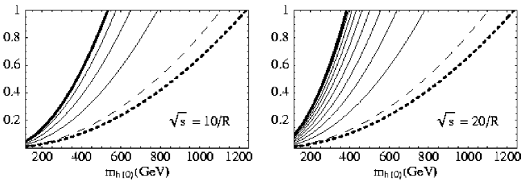
Figure 1: The plots show for which value of $m_{h(0)}$ the tree level unitarity bound in eq.(8) is violated. The thick dotted line stands for the SM ($n=0$) results only from the $W_{L\,(0)}^{+}W_{L\,(0)}^{-}$ elastic scattering, eq.(5), whereas the dashed line includes also the $h_{(0)}h_{(0)}$, $Z_{L\,(0)}Z_{L\,(0)}$ coupled states in eq.(8). The continuous lines correspond to considering in eq.(8) the first, second, etc… KK excitations of the previous states. The thick continuous line shows the complete calculation including all the kinematically allowed states, which, for $\sqrt{s}=10/R$ and $20/R$, are 4 and 9 KK levels, respectively. Note that for any $m_{h(0)}$ there is a $\sqrt{s}$ above which tree level unitarity is violated. The energies have been chosen below the expected scale where the gauge coupling becomes non-perturbative, $30/R$ [4].

In Figure 1 we show for what $m_{h(0)}$ value the unitarity bound in eq.(8) is violated for a given energy and compactification radius. The curves represent the tree level approximation to the left hand side of the inequality, so that when they are larger than one show a violation of the unitarity bound already by considering only two-particle states. The thick dotted line corresponds to the analysis considering just the single $W_{L\,(0)}^{+}W_{L\,(0)}^{-}\rightarrow W_{L\,(0)}^{+}W_{L\,(0)}^{-}$ amplitude. The dashed line would be the bound including the other zero modes, that is, the SM result for the left hand side of eq.(8). The continuous lines represent the change on eq.(8) if one considers the coupled unitarity bound including the first KK level, the second, etc… Of course, one should consider all the KK states that can be produced up to the energy under consideration, and that corresponds to the thick continuous line. We can notice that the unitarity bound can be reduced drastically by considering an additional extra dimension. Note that as we have previously shown, for any $m_{h(0)}$ there is a $\sqrt{s}$ above which tree level unitarity is violated.

Figure 2: The plots show the energies where the tree level calculation violates the coupled channel unitarity bound eq.(8). The thick dotted and dashed lines correspond to the SM bounds without KK excitations just for the single channel, eq.(5), or coupled channel case, eq.(8). Each continuous line represents the contribution of the new KK states that open as the energy increases. The total result considering all the accessible KK level is the thick continuous line.

In Figure 2, we show the energy at which tree level unitarity is violated for a given Higgs mass $m_{h(0)}$. Roughly speaking, this means that beyond that point perturbation theory is no longer valid. However, let us remark that the saturation of the unitarity bounds is also an indication that the model has become strongly interacting. For practical purposes this can be considered the case when the tree level calculation provides more than half of the unitarity bound. Again the thick dotted and dashed lines correspond to considering the SM fields in the single or coupled channel case, respectively, whereas the continuous lines represent the contribution to the unitarity bound of each new level of KK accessible excitations at that energy. The total result, considering all accessible KK lavels corresponds to the thick continuous line. Note that in the upper row of figures, we have chosen a compactification radius $R=1/(500\,$GeV$)$ and Higgs masses which are within the presently $90\%$ allowed region in 5D universal extra dimensional models [3, 4]. The lower row, with $R=1/(3\,$TeV$)$ is the typical value for models with fermions localized on the brane [2].

In Figure 3, for different values of $R$, we show contour plots in the $\sqrt{s},m_{h(0)}$ plane, of Unit${}_{W_{L\,(0)}^{+}W_{L\,(0)}^{-}\rightarrow W_{L\,(0)}^{+}W_{L\,(0)}^{-}}$ in eq.(8). The white area represents the region where the tree level calculation violates the unitarity bound already considering two-particles states. Within the gray areas, the two-body amplitudes add to more than half of the unitarity bound, suggesting that the theory becomes strongly interacting.

Again, we can see in the $R=1/(500\,$GeV$)$ plots that the models can become strongly interacting within the reach of the LHC. This could be of relevance since the scale where the gauge coupling becomes non-perturbative in 5D universal extra dimension models has been estimated around $30/R$ [4]. Within our approach it is not the running of the coupling, but the proliferation of states and the fact that the coupling is not suppressed when increasing the KK level, what drives the tree level unitarity violation. If higher orders are to modify this behavior they should be comparable to the tree level and the theory becomes strongly interacting. As a matter of fact, we see in Fig.3 that the models can become strongly interacting much before the scale of 30/R, depending on the Higgs mass. For instance, by looking at Figure 3 in the $R=1/(500\mbox{GeV})$ case, the gauge coupling would become nonperturbative at approximately $30/R=15\,$TeV, but we see that for $m_{h(0)}=500\,$GeV the theory violates tree level unitarity already at 5 TeV and becomes strong below 3 TeV. We recall once again that we are only considering two-particle states, but the many-particle states, since they always add in eq.(8), would even provide a stronger bound.

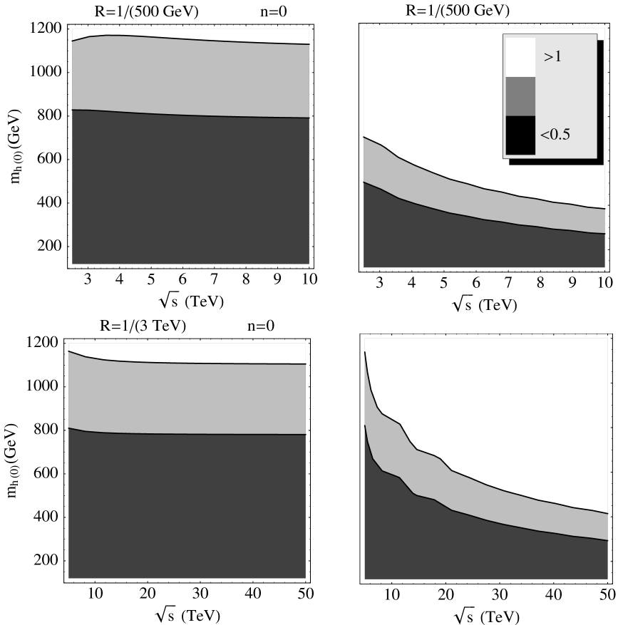
Figure 3: The white areas represent the regions of the $(\sqrt{s},m_{h(0)})$ plane where the tree level calculation violates the unitarity bound. The gray areas represent the regions where Unit${}_{W_{L\,(0)}^{+}W_{L\,(0)}^{-}\rightarrow W_{L\,(0)}^{+}W_{L\,(0)}^{-}}$ in eq.(8) is larger than $0.5$, and suggest a strongly interacting regime. We show, the bounds obtained using only the SM fields ($n=0$), and those including the KK excitations.

Let us finally get a crude estimate of an energy for which the tree level calculation violates unitarity for a given $m_{h(0)}$. It will not be as tight as the explicit calculation shown above but in contrast will be very easy to implement.

First, if we consider $s\gg m_{h(0)}^{2}$, we can approximate the modulus of the partial waves just by the constant terms in eq.(18), which correspond to the quartic couplings. That this is a fairly good approximation can be explicitly checked in the partial waves given in the appendix, since the trilinear terms are suppressed by s-channel propagators, $1/(s-m_{h(0)}^{2})$ or $m_{h(0)}^{2}/s$ factors in the logarithmic terms that appear from the angular integration of $t$ and $u$ channel propagators. The error in this approximation is $20\%$ for $\sqrt{s}\simeq 5m_{h(0)}$ and decreases very fast. Remarkably, within this approximation, the partial waves for KK modes are exactly a copy of the SM ones. Each new KK level that opens up adds an additional copy. Note that there is not any suppression in the amplitudes when increasing the KK level.

Second, we have to count how many KK levels are effectively opened for a given energy. But for small differences, all the new particles in a KK level are characterized by a typical mass scale $m_{(n)}\simeq n/R>m_{h(0)}$. As we have already commented, the two-particle phase space grows rather rapidly. In particular, it can be checked that the phase space $\sigma_{n}=\sqrt{1-4m^{2}_{(n)}/s}$ of the two-particle state of the $n$-th KK level is of order one already at $\sqrt{s}>3m_{(n)}$. Note that we are neglecting all the states that could have just opened at that energy but are below $\sqrt{s}>3m_{(n)}$ and would have contributed positively to the bound. Thus, at that energy, we have the following two-particle states available: the usual SM ones, plus $n$ KK copies, which as we have seen have the same amplitudes. For those energies, we can then approximate the sum of two-particle states in eq.(8) as

$${\rm Unit}_{W_{L\,(0)}^{+}W_{L\,(0)}^{-}\rightarrow W_{L\,(0)}^{+}W_{L\,(0)}^{-}}\simeq\frac{5m_{h}^{2}G_{F}}{16\pi\sqrt{2}}\sum_{k=0}^{n}\sigma_{k}\simeq\frac{5m_{h}^{2}G_{F}}{16\pi\sqrt{2}}(n+1)\leq 1.$$ (19)

Thus, we arrive to the following crude bound: given any value of the Higgs mass $m_{h(0)}$, for energies larger than

$$\sqrt{s}\simeq\frac{3}{R}\left[\frac{16\pi\sqrt{2}}{5\,G_{F}\,m^{2}_{h(0)}}-1\right]\quad(s\gg m^{2}_{h(0)}),$$ (20)

tree level unitarity is violated. This bound is only applicable for $\sqrt{s}>m_{h(0)}$.y We have checked that this formula gives a reasonably accurate bound within $10\%$ of the complete calculation. Indeed, we see by comparing Fig.4.a with 3.b that the 5D results obtained with the estimate, eq.(20), are in good agreement with the complete tree level calculation eq.(8).

5 Additional extra dimensions

In the previous section we have obtained very strong tree level unitarity bounds when we added to the SM an additional tower of KK states coming from a compactified extra dimension. These contributions are always present when new states become available, and if the couplings to these new states are not suppressed when increasing the KK level, they can be comparable to those of the SM fields. We have seen that for sufficiently high energies and just one extra dimension, the number of two-particle states grows linearly with $\sqrt{s}$. However, we will see next that when considering more than one extra dimension, the number of states grows much faster, and the unitarity bounds become extraordinarily much tighter. This result is of relevance in the context of universal extra dimensions [4], where the problem of proton instability has been solved precisely in six dimensions [10].

This is particularly simple to see if we just add another dimension with the same compactification radius to the previous model. In such a case, instead of a generic $\alpha_{(n)}$ tower of states of two particles with mass $m_{(n)}\simeq n/R$, we have $\alpha_{(n_{1},n_{2})}$ states of two particles with mass $m_{(n_{1},n_{2})}\simeq\sqrt{n_{1}^{2}+n_{2}^{2}}/R$. Note that we are now writing explicitly the KK level, because in the models of interest there is no mixing among the modes with different KK numbers.

As before we are interested in two-body states that can be produced at tree level from a state with two zero-level particles. In Table 1, we find the states made of two particles with the same KK numbers, available as the level number $n\geq n_{1},n_{2}$ increases.

KK level	5D	6D
0th	$\alpha_{(0)}$	$\alpha_{(0,0)}$
1st	$\alpha_{(1)}$	$\alpha_{(1,0)}$, $\alpha_{(0,1)}$, $\alpha_{(1,1)}$
2nd	$\alpha_{(2)}$	$\alpha_{(2,0)}$, $\alpha_{(0,2)}$, $\alpha_{(2,1)}$, $\alpha_{(1,2)}$, $\alpha_{(2,2)}$
3rd	$\alpha_{(3)}$	$\alpha_{(3,0)}$, $\alpha_{(0,3)}$, $\alpha_{(3,1)}$, $\alpha_{(1,3)}$, $\alpha_{(2,3)}$, $\alpha_{(3,2)}$, $\alpha_{(3,3)}$
4th	$\alpha_{(4)}$	9 states
…	…	…
nth	$\alpha_{(n)}$	2n+1 states

Table 1: States made of two particles with the same KK numbers, available as each KK level opens for one or two $S^{1}/Z_{2}$ extra dimensions in the model of section 3.

We see that for the 5D case we had $n+1$ states at the $n$th level whereas for the 6D case we have $(n+1)^{2}$. Note that for $n\geq 3$, when the $(n,n)$ state is opened there can also be additional opened states from the $n+1$ level, for instance the $(n+1,0)$, which is lighter than $(n,n)$. But considering only those up to $n\geq n_{1},n_{2}$ we can easily count the number of states and thus reobtain the crude estimate in eq.(20) changing the number of states available

$${\rm Unit}_{W_{L\,(0)}^{+}W_{L\,(0)}^{-}\rightarrow W_{L\,(0)}^{+}W_{L\,(0)}^{-}}\simeq\frac{5m_{h}^{2}G_{F}}{16\pi\sqrt{2}}(n+1)^{2}\leq 1.$$ (21)

As usual, we have restricted ourselves to two-body states because they are very easy to calculate, but all the other accessible states that we have not counted always add to the equation above and hence would have given an even stronger bound on the Higgs mass. Next, we note that the phase space of the heaviest two-particle $nth$-level state, which is made of two $\alpha_{(n,n)}$ fields of mass $m_{(n,n)}\simeq\sqrt{2}n/R$, is of order one when $\sqrt{s}\simeq 3m_{(n,n)}/R$ or larger. Thus, we now expect a violation for energies above or around

$$\sqrt{s}\simeq\frac{3\sqrt{2}}{R}\left[\sqrt{\frac{16\pi\sqrt{2}}{5\,G_{F}\,m^{2}_{h(0)}}}-1\right].$$ (22)

Hence, in this case we can consider eq.(22) more conservative than the analogous in 5D, eq.(20). If we had also considered opened states beyond the $n$th level, like $(n+1,0)$, the unitarity bound above would even be tighter (but the counting of states would be more complicated).

The generalization to $d$ additional dimensions is straightforward by changing $(n+1)^{2}$ by $(n+1)^{d}$ in eq.(21). Of course, the model could be more complicated and have different compactification radius for each dimension, in such a case, if for a given energy the KK states associated to the first extra dimensions are accessible up to the $n_{1}$ level and those of the next up to $n_{2}$ , etc… we have to substitute $(n+1)^{d}$ by $(n_{1}+1)(n_{2}+1)...(n_{d}+1)$.

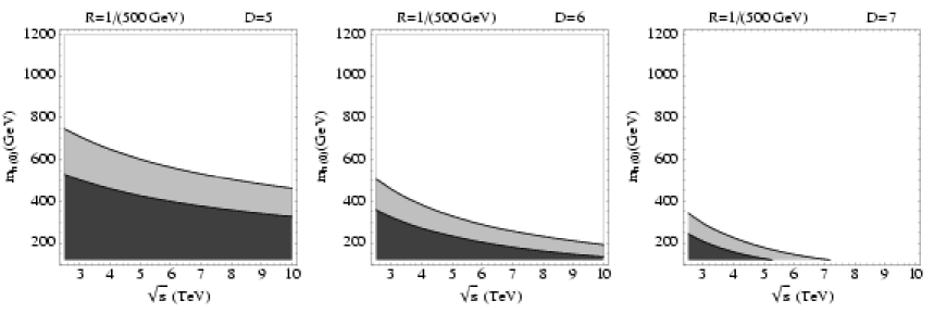
Figure 4: The white areas represent the regions of the $(\sqrt{s},m_{h(0)})$ plane where the tree level estimate, eqs.(20),(22), violate the unitarity bound for 5, 6 or 7 dimensions. The gray areas represent the regions where Unit_α→α in eq.(8) is larger than $0.5$, and suggest a strongly interacting regime. By comparing Fig.4.a with 3.b it can be noticed that the 5D results obtained with the estimate are in good agreement with the complete tree level calculation.

In Fig.4 we show the results of using the crude estimate for the tree level unitarity violation, eqs.(20) and (22). For illustration we have chosen again a value of $1/R$ which is presently allowed in the 5D and 6D universal extra dimension context. For the 7D results we have simply replaced $(n+1)^{2}$ by $(n+1)^{3}$ in eq.(22) as explained above. It can be noticed that by increasing the number of dimensions where the scalar sector lives, the violation of tree level unitarity can be dramatic within the LHC reach, which could be of considerable phenomenological relevance.

6 Conclusions

In this work we have presented a very simple method to obtain unitarity bounds at finite energy when a large number of states are available. These kind of bounds are very relevant in order to determine the energy at which perturbation theory breaks down for a given set of parameters of the theory. These bounds also suggest the condition under which the theory becomes strongly interacting. The approach relies on the well known formalism for coupled channel partial wave unitarity. Thus, it can be applied generically and avoids the calculation of large determinants of complicated functions.

Our initial motivation to look for this kind of method are the extra dimensional extensions of the SM, which introduce an infinite tower of Kaluza Klein states that could saturate the unitarity bounds much before than in the familiar four-dimensional SM. Although the bounds obtained from this formalism can be applied to particles with any spin, we have illustrated this effect with a SM whose scalar sector is located in the bulk. Incidentally this one as well as other similar models where the self-couplings of the scalar potential are not suppressed for higher Kaluza Klein states have received some recent phenomenological interest.

We have indeed shown that within these models, shortly after a new KK level can be produced, their contribution to the unitarity bound is of the same order of that of the SM, thus changing the usual bounds dramatically as soon as several KK level are opened. In certain cases, this would imply that the model becomes strongly interacting much before the usual expectations, thus casting doubts about simple perturbative calculations or estimates. Let us finally remark the possible phenomenological interest of these bounds, since within some valid regions of parameter space, they could well suggest a strongly interacting regime within the reach of the next generation of colliders.

Appendix A Appendix

To study the tree level unitarity bounds we are interested in the scattering of longitudinal gauge bosons $W^{+}_{L(0)}W^{-}_{L(0)}$ at leading order in $g$ and $g^{\prime}$. In the SM at tree level this state is also coupled to $Z_{L(0)}Z_{L(0)}$ and $h_{(0)}h_{(0)}$. Using the ET, at high energies, $\sqrt{s}>m_{V(0)}$ the longitudinal gauge boson amplitudes can be replaced by their corresponding Goldstone boson amplitudes. Using the 5D potential in eq.(10) and integrating out the fifth dimension as explained in the text, we find in the Landau gauge $\xi\rightarrow 1$:

$$t^{J=0}_{G^{+}_{(0)}G^{-}_{(0)}\rightarrow G^{+}_{(0)}G^{-}_{(0)}}=\frac{-G_{F}m^{2}_{h(0)}}{8\pi\sqrt{2}}\left[2+\frac{m^{2}_{h(0)}}{s-m^{2}_{h(0)}}-\frac{m^{2}_{h(0)}}{s}\log\Big{(}1+\frac{s}{m^{2}_{h(0)}}\Big{)}\right],$$ (23)

$$t^{J=0}_{G^{+}_{(0)}G^{-}_{(0)}\rightarrow G^{Z}_{(0)}G^{Z}_{(0)}}=\frac{-G_{F}\,m^{2}_{h(0)}}{16\pi}\left[1+\frac{m^{2}_{h(0)}}{s-m^{2}_{h(0)}}\right],$$ (24)

$$t^{J=0}_{G^{+}_{(0)}G^{-}_{(0)}\rightarrow h_{(0)}h_{(0)}}=\frac{-G_{F}\,m^{2}_{h(0)}}{16\pi}\left[1+\frac{3m^{2}_{h(0)}}{s-m^{2}_{h(0)}}+\frac{4m^{2}_{h(0)}}{s\,\sigma_{h(0)}}\log\Big{(}\frac{s-2m^{2}_{h(0)}-s\,\sigma_{h(0)}}{2m^{2}_{h(0)}}\Big{)}\right],$$ (25)

where $\sigma_{\Phi}=\sqrt{1-4m^{2}_{\Phi}/s}$ and we have already included the $1/\sqrt{2}$ factor for identical particles. Incidentally, they are the same as in the SM [7].

In addition, in 5D the longitudinal gauge bosons also couple to their KK excitations as well as to $h_{(n)}h_{(n)}$, $a^{+}_{(n)}a^{-}_{(n)}$, $a^{Z}_{(n)}a^{Z}_{(n)}$. In [8] we have already shown that the corrections to the SM results from the longitudinal KK gauge excitations are suppressed as $O(m_{W}^{4}/R^{4})$ and can be also neglected on a first approximation. However, we need the following partial waves,

$$t^{J=0}_{G^{+}_{(0)}G^{-}_{(0)}\rightarrow a^{+}_{(n)}a^{-}_{(n)}}=\frac{-G_{F}m^{2}_{h(0)}}{8\pi\sqrt{2}}\left[2+\frac{m^{2}_{h(0)}}{s-m^{2}_{h(0)}}-\frac{m^{2}_{h(0)}}{s\sigma_{a^{\pm}(n)}}\log\left(\frac{2m^{2}_{a^{\pm}(n)}-2m^{2}_{h(n)}-s(1+\sigma_{a^{\pm}(n)})}{2m^{2}_{a^{\pm}(n)}-2m^{2}_{h(n)}-s(1-\sigma_{a^{\pm}(n)})}\right)\right],$$

$$t^{J=0}_{G^{+}_{(0)}G^{-}_{(0)}\rightarrow a^{Z}_{(n)}a^{Z}_{(n)}}=\frac{-G_{F}\,m^{2}_{h(0)}}{16\pi}\left[1+\frac{m^{2}_{h(0)}}{s-m^{2}_{h(0)}}\right],$$

$$t^{J=0}_{G^{+}_{(0)}G^{-}_{(0)}\rightarrow h_{(n)}h_{(n)}}=\frac{-G_{F}\,m^{2}_{h(0)}}{16\pi}\left[1+\frac{3m^{2}_{h(0)}}{s-m^{2}_{h(0)}}-\frac{2m^{2}_{h(0)}}{s\,\sigma_{h(n)}}\log\left(\frac{2m^{2}_{h(n)}-2m^{2}_{a^{\pm}(n)}-s(1+\sigma_{h(n)})}{2m^{2}_{h(n)}-2m^{2}_{a^{\pm}(n)}-s(1-\sigma_{h(n)})}\right)\right].$$

Note that all these amplitudes for the $a^{V}_{(n)}$ are obtained replacing $\omega_{(n)}^{V}\rightarrow c^{{}_{V}}_{n}\,\,a^{V}_{(n)}$ in the Higgs potential after the integration of the 5th dimension. When deriving these amplitudes we have considered the leading order in $c^{{}_{V}}_{n}=(1-m^{2}_{V(0)}R^{2}/(2n^{2})+\cdots)$ , thus neglecting $O(m_{V(0)}^{2}R^{2})$. In the worst case considered in our calculations $m_{V(0)}^{2}R^{2}\simeq(90/500)^{2}$, less than a 4%.

References

- [1] I. Antoniadis, Phys. Lett. B 246 (1990) 377; A. Pomarol and M. Quirós, Phys. Lett. B 438 (1998) 255; I. Antoniadis, S. Dimopoulos, A. Pomarol and M. Quirós, Nucl. Phys. B 544 (1999) 503; A. Delgado, A. Pomarol and M. Quirós, Phys. Rev. D 60 (1999) 095008.
- [2] I. Antoniadis and K. Benakli, Phys. Lett. B 326 (1994) 69; P. Nath and M. Yamaguchi, Phys. Rev. D 60 (1999) 116004; W. J. Marciano, Phys. Rev. D 60 (1999) 093006; M. Masip and A. Pomarol, Phys. Rev. D 60 (1999) 096005; T. G. Rizzo and J. D. Wells, Phys. Rev. D 61 (2000) 016007; A. Strumia, Phys. Lett. B 466 (1999) 107; R. Casalbuoni, S. De Curtis, D. Dominici and R. Gatto, Phys. Lett. B 462 (1999) 48; C. D. Carone, Phys. Rev. D 61 (2000) 015008; A. Delgado, A. Pomarol and M. Quirós, JHEP 0001 (2000) 030.A. Muck, A. Pilaftsis and R. Ruckl, Phys. Rev. D 65 (2002) 085037.
- [3] R. Barbieri, L. J. Hall and Y. Nomura, Phys. Rev. D 63 (2001) 105007;
- [4] T. Appelquist, H. C. Cheng and B. A. Dobrescu, Phys. Rev. D 64 (2001) 035002.T. Appelquist and H. U. Yee, Phys. Rev. D 67 (2003) 055002.
- [5] R. S. Chivukula, D. A. Dicus and H. J. He, Phys. Lett. B 525 (2002) 175; R. S. Chivukula and H. J. He, Phys. Lett. B 532 (2002) 121.
- [6] J. M. Cornwall, D. N. Levin and G. Tiktopoulos, Phys. Rev. D10 (1974) 1145; C. E. Vayonakis, Lett. Nuovo Cim. 17 (1976) 383; M. S. Chanowitz and M. K. Gaillard Nucl. Phys. B261 (1985) 379; G. K. Gounaris, R. Kogerler and H. Neufeld, Phys. Rev. D34 (1986) 3257; Y. P. Yao and C. P. Yuan, Phys. Rev. D38 (1988) 2237; J. Bagger and C. Schmidt, Phys. Rev. D41 (1990) 264; H.J. He, Y. P. Kuang, and X. Li Phys. Rev. Lett. 69 (1992) 2619.
- [7] B. W. Lee, C. Quigg and H. B. Thacker, Phys. Rev. D 16 (1977) 1519.
- [8] S. De Curtis, D. Dominici and J. R. Pelaez, Phys. Lett. B 554 (2003) 164.
- [9] R.G. Newton,”Scattering Theory of waves and Particles”, 2nd ed. Texts and Monographs in Physics. Springer Verlag NY (1982). A. Dobado, A. Gomez-Nicola, A. Maroto and J. R. Pelaez, “Effective Lagrangians For The Standard Model”, Texts and Monographs in Physics. Springer Verlag NY (1997).
- [10] T. Appelquist, B. A. Dobrescu, E. Ponton and H. U. Yee, Phys. Rev. Lett. 87 (2001) 181802