CERN-TH/2002-371
UPRF-2002-19
December 2002

Heavy-Quark Fragmentation

Matteo Cacciari$\;{}^{(1)}$  and  Einan Gardi$\;{}^{(2,3)}$

⁽¹⁾ Dipartimento di Fisica, Università di Parma, Italy,

and INFN, Sezione di Milano, Gruppo Collegato di Parma

⁽²⁾ TH Division, CERN, CH-1211 Geneva 23, Switzerland

⁽³⁾ Institut für Theoretische Physik, Universität Regensburg,

D-93040 Regensburg, Germany

Abstract: We study perturbative and non-perturbative aspects of heavy-quark fragmentation into hadrons, emphasizing the large-$x$ region, where $x$ is the energy fraction of the detected hadron. We first prove that when the moment index $N$ and the quark mass $m$ get large simultaneously with the ratio $N\Lambda/m$ fixed, the fragmentation function depends on this ratio alone. This opens up the way to formulate the non-perturbative contribution to the fragmentation function at large $N$ as a shape function of $m(1-x)$ which is convoluted with the Sudakov-resummed perturbative result. We implement this resummation and the parametrization of the corresponding shape function using Dressed Gluon Exponentiation. The Sudakov exponent is calculated in a process independent way from a generalized splitting function which describes the emission probability of an off-shell gluon off a heavy quark. Non-perturbative corrections are parametrized based on the renormalon structure of the Sudakov exponent. They appear in moment space as an exponential factor, with a leading contribution scaling as $N\Lambda/m$ and corrections of order $(N\Lambda/m)^{3}$ and higher. Finally, we analyze in detail the case of $B$-meson production in $e^{+}e^{-}$ collisions, confronting the theoretical predictions with LEP experimental data by fitting them in moment space.

1 Introduction

The fragmentation process, in which an energetic quark becomes a hadron, is one of the most interesting processes in the physics of the strong interaction, making an immediate link between the perturbative regime and confinement. The case of heavy (bottom and, possibly, charm) quark fragmentation is special in that the quark mass $m$, being significantly larger than the QCD scale $\Lambda$, allows one better theoretical control. In particular, the mass provides a physical infrared cutoff for collinear radiation making the fragmentation process accessible to perturbative methods.

The methodology to describe processes involving fragmentation is based on factorization. In general “factorization” refers to the separation of the physical process into subprocesses which are mutually incoherent each depending on a separate scale. In practice this term is mainly used in the context of separating the perturbative and non-perturbative contributions [1]. The general procedure (see e.g. [2]) is then to compute the cross section perturbatively and complement it by a convolution with a non-perturbative fragmentation function describing the softening of the heavy-quark momentum as it goes through the hadronization process.

Experimentally, observables involving bottom fragmentation are particularly important. New experimental data have recently provoked much debate [3, 4, 5] about the accuracy of predictions for $B$-meson hadroproduction obtained by convoluting the perturbative cross section for bottom quarks with commonly used phenomenological models [6, 7]. There exist many different viable implementations of a perturbative calculation for heavy-quark production using massive or massless quarks, different orders in $\alpha_{s}$, soft-gluon resummation, Monte-Carlo simulations, etc. The phenomenology is particularly intricate because the parameters of the non-perturbative fragmentation function determined by fits to data are very sensitive to the details of the perturbative description used. Consequently the application of these functions requires to use the same kind of perturbative description with which they were determined.

On the theoretical side progress has been made at both the perturbative [8, 9, 10, 12, 11, 13] and the non-perturbative [14, 15] frontiers. Nevertheless, the most pressing questions have not been answered, namely

• How should the non-perturbative fragmentation function be parametrized, in particular in the region where the energy fraction $x$ of the detected meson is large? This is especially important since the distribution peaks at large $x$.

• Is this function really universal? e.g. can the parameters be fixed from data on bottom fragmentation in $e^{+}e^{-}$ annihilation and used in various observables in hadron colliders?

Answering these questions requires deep insight into the non-perturbative regime. However, a crucial step in addressing them is making a clear and sensible separation between the perturbative and the non-perturbative aspects and then dealing with both. Most previous work on the subject is sharply divided between a purely perturbative treatment, which concentrated on resumming the dominant perturbative corrections [8, 10, 13], and a purely non-perturbative approach, which disregarded the perturbative aspects. The latter was either phenomenological in essence [6, 7], or relied on general considerations such as the quark-mass expansion [14], but avoided the large-$x$ region. None of these approaches has led to a satisfactory description of the fragmentation function at large $x$. This region is characterized by large perturbative and non-perturbative effects, so both aspects need to be addressed.

Owing to soft gluon radiation the perturbative result at any given order diverges for $x\longrightarrow 1$. This makes Sudakov resummation an essential ingredient in the description of heavy-quark fragmentation [13]. While important, Sudakov resummation (see e.g. Fig. 8 below) does not lead, by itself, to a phenomenologically acceptable description of the cross section: it is much too hard and eventually becomes negative near $x=1$. Non-perturbative corrections are required.

It is well known that due to renormalons [16] the separation between the perturbative and non-perturbative regimes is arbitrary. This means [17, 18, 19, 20] on the one hand that great care should be taken in controlling the accuracy of the resummed perturbative expansion whenever power-corrections are important but, on the other hand, that some insight on non-perturbative physics can be gained based on perturbation theory. Under the assumption that the renormalon contribution dominates, this information can be used to parametrize the non-perturbative corrections. Realizing this, Nason and Webber [15] have used the structure of infrared renormalons to determine the parametric form of the leading power correction to the heavy-quark fragmentation function in the large-$N$ limit, where $N$ is the moment (at large $N$, the $N$-th moment is sensitive to $x\sim 1-1/N$). They found that it should scale as $N\Lambda/m$. This is an important result, which we further establish and generalize here.

Based on the quark-mass expansion of [14] and on a general representation of the fragmentation function at large $N$ in terms of a non-local lightcone matrix element at a large lightcone separation (which follows directly from the definition [1]), we prove that in the limit where $N$ and $m$ become large simultaneously, the fragmentation function depends only on the ratio $N\Lambda/m$ up to corrections of order $1/N$. This opens up the way to resum these non-perturbative corrections into a function of a single variable $N\Lambda/m$. The corresponding function in momentum fraction space depends on $m(1-x)$. This function is convoluted with the resummed perturbative distribution, thereby introducing a shift and a deformation of the shape by non-perturbative effects. For this reason it is called a “shape function”. The scaling property of the fragmentation function was known before (see [2] are refs. therein), but a formal proof based on the properties of the hadronic matrix element was never established.

Stepping forward from a leading, additive power correction to a shape function, which is a multiplicative correction in moment space, is essential for describing differential cross sections near a kinematic threshold [21, 22, 23, 18]. Shape-function based phenomenology has been developed particularly in the context of event-shape distributions in $e^{+}e^{-}$ annihilation [21, 22, 24, 18] where it has proven very useful. The same methodology can be applied to a large class of observables.

Our approach to the problem of heavy-quark fragmentation is based on perturbation theory. Instead of parametrizing the differential distribution for the production of a heavy meson from a heavy quark, we start off with a perturbative calculation of this distribution. The result is then modified by power corrections through a convolution with a shape function whose parametric form is deduced from the ambiguity in the perturbative result. A convolution of a perturbative (possibly Sudakov-resummed) heavy-quark distribution with a phenomenological non-perturbative function has been commonly used in describing heavy-meson production. However, there are deep conceptual differences between our approach and the common practice: a) the resummation we perform, which focuses on the effect of the running coupling in the Sudakov exponent, is aimed at power accuracy, so that the separation between the perturbative and non-perturbative components is power-like; b) since the functional form of the non-perturbative component is constructed according to the ambiguity of the perturbative one, it should not be considered as a phenomenological model; c) since we only rely on QCD, there is room for a systematic improvement of both the perturbative and the non-perturbative ingredients.

We concentrate in this paper on the large-$x$ region, neglecting power corrections which are suppressed by the energy of the quark, ${\cal O}(\alpha_{s}^{2})$ perturbative corrections that are not logarithmically enhanced, as well as power corrections in $\Lambda/m$ which are not enhanced by the same power of $N$. Consequently, our description of the first few moments is of limited accuracy.

Attempting to reach power accuracy at large $x$, our resummation program is based on Dressed Gluon Exponentiation (DGE). Calculating the Sudakov exponent as an integral over the running coupling (a renormalon sum) we refrain from making a truncation at some fixed logarithmic accuracy. The advantages of this methodology have already been discussed in detail in [18, 19, 20]. However, some new features appear in the case of the fragmentation function owing to the low scale $m/N$. As we will see, the perturbative expansion of the Sudakov exponent reaches the minimal term already at the next-to-leading-log (NLL) and a rather large difference exists between truncation of the series at this order and a principal-value (PV) regularization of the Borel integral. The latter is advantageous as a basis for the parametrization of power corrections, being it free of Landau type singularities and having a smooth behavior at large $N$.

Although data analysis is performed here only in one case, namely the semi-inclusive cross section for $B$-meson production in $e^{+}e^{-}$ annihilation at LEP, we are guided by the hypothesis that the fragmentation function is universal, an idea that guided many phenomenological applications in recent years [25, 26, 27, 28, 3]. With universality in mind, we write our resummation formulae for the cross section in a fully factorized form, where subprocesses (such as the fragmentation function) depending on distinct external scales appear as independent entities. This type of factorization is not restricted to the resummed perturbation theory, but instead it becomes a property of the full subprocess including the non-perturbative contributions.

The paper is organized as follows. Section 2 recalls the standard definition of the fragmentation function and then deals with the heavy-quark fragmentation function in the large-$N$ limit on general grounds. Section 3 summarizes a process-independent, all-order calculation of the heavy-quark fragmentation function in the large-$\beta_{0}$ limit. It is based on computing a generalized splitting function describing an off-shell gluon emission off a heavy quark. We then analyze the Borel singularity of the fragmentation function and construct an ansatz for the shape function. Section 4 specializes to the case of $e^{+}e^{-}$ annihilation. We begin by performing a renormalon calculation for the differential cross section of the entire process and then identifying the contributions which are enhanced near $x=1$. Isolating the fragmentation subprocess we recover the result of Sec. 3 and interpret the remaining subprocesses which form the coefficient function. In Sec. 5 we discuss the phenomenological implications of our results and confront them with LEP data on bottom production in $e^{+}e^{-}$ annihilation. Section 6 summarizes our conclusions.

2 Heavy quark fragmentation in the large-$x$ limit

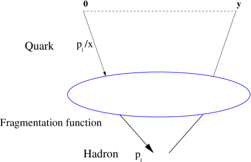
Figure 1: The definition of the fragmentation function. The dashed line represents a path-ordered exponential.

The leading-twist quark fragmentation function, corresponding to the probability of a quark to fragment into a hadron with a longitudinal momentum fraction $0<x<1$ (see fig. 1), is defined by [1],

$$D(x;\mu^{2})\equiv\frac{1}{2\pi\,x}\int_{-\infty}^{\infty}\frac{dy_{-}}{y_{-}}\,\exp(i{p_{1}}y/x)\,F(p_{1}y;\mu^{2}),$$ (1)

where $F(p_{1}y;\mu^{2})$ stands for the following non-local matrix element

$$F(p_{1}y;\mu^{2})\equiv\frac{1}{4\,N_{c}}\,\sum_{X}\,{\rm Tr}\left\{\langle 0|\mbox{$y$\raisebox{0.43057pt}{$/$}}\Psi(y)|H(p_{1})+X\rangle\langle H(p_{1})+X|\overline{\Psi}(0)|0\rangle_{\mu^{2}}\right\},$$ (2)

renormalized at $\mu^{2}$, averaged over spin and color of the initial quark and summed over all final states containing a hadron $H$ with momentum $p_{1}$. We choose light-cone coordinates such that $p_{1}$ has a large “$+$” component, while $y$ is a light-like vector in the “$-$” direction ($y_{+},y_{\perp}\equiv~{}0$). Path-ordered exponential factors are required to make (2) gauge invariant. However, since we will eventually use the light-cone gauge $y\cdot A=0$ where these factors become trivial, we will not write them explicitly.

While this definition applies to fragmentation of both light and heavy quarks, there is a fundamental difference in our ability to use the theory in the two cases. In the case of light quarks, only the $\mu^{2}$ evolution of the matrix element is calculable, whereas for heavy quarks with mass $m\gg\Lambda$ the matrix element itself and thus $D(x,m^{2};\mu^{2})$ can be calculated perturbatively, while non-perturbative effects can be treated systematically as corrections. The matrix element can be calculated since $m^{2}$ provides a natural cutoff for collinear gluon radiation. It also provides a natural scale for renormalization of the operator $\mu^{2}=m^{2}$, serving as a factorization scale in a generic hard process. In the following we will use simplified notation $D(x,m^{2};\mu^{2}=m^{2})=D(x,m^{2})$ and $F(p_{1}y,m^{2};\mu^{2}=m^{2})=F(p_{1}y,m^{2})$.

By matching the general definition given above onto the heavy-quark effective theory, Jaffe and Randall [14] have shown that in the large $m$ limit the non-local matrix element in (2) can be written in terms of a function of the product $(p_{1}y)\,\bar{\Lambda}/m$ up to corrections which are suppressed by $\bar{\Lambda}/m$:

$$\frac{F(p_{1}y,m^{2})}{p_{1}y}\,\longrightarrow\,\exp\left(-i{p_{1}}y\right)\,\left[{\cal F}(p_{1}y\,\bar{\Lambda}/m)+{\cal O}(\bar{\Lambda}/m)\right].$$ (3)

Physically $\bar{\Lambda}$ appears as the energy of the light quark (including the binding energy) in a meson, corresponding to $M-m$, where $M$ and $m$ are the heavy meson and quark masses, respectively. This particular dependence of $F(p_{1}y,m^{2})$, which follows directly from QCD, has a phenomenological significance: it constrains possible models for the parametrization of the heavy-quark fragmentation. Due to the difficulty to distinguish between perturbative and non-perturbative corrections at large $x$, Jaffe and Randall exclusively concentrate in their analysis on the first few Mellin moments of the $D(x,m^{2})$,

$$\tilde{D}(N,m^{2})=\int_{0}^{1}dx\;x^{N-1}D(x,m^{2}).$$ (4)

As explained in the introduction, the behavior of the fragmentation function in the large-$x$ limit is particularly interesting both from a purely theoretical point of view and for practical applications. As we show in the following sections, if properly resummed, perturbation theory does provide a basis for the analysis of heavy-quark fragmentation at large $x$, so long as $m(1-x)\mathrel{\mathchoice{\vbox{\offinterlineskip\halign{$\m@th\displaystyle\hfil#\hfil$\cr>\crcr\sim\crcr} }}{\vbox{\offinterlineskip\halign{$\m@th\textstyle\hfil#\hfil$\cr>\crcr\sim\crcr} }}{\vbox{\offinterlineskip\halign{$\m@th\scriptstyle\hfil#\hfil$\cr>\crcr\sim\crcr} }}{\vbox{\offinterlineskip\halign{$\m@th\scriptscriptstyle\hfil#\hfil$\cr>\crcr\sim\crcr} }}}{\bar{\Lambda}}$. Of course, power corrections can be ignored only if $m(1-x)\gg\bar{\Lambda}$, so in practice the perturbative calculation must be supplemented by non-perturbative corrections.

While phenomenological parameters are definitely needed for a precise description of (1), it is important to constrain theoretically its functional form as much as possible. In the rest of this section we show how the large-$x$ behaviour of $D(x,\mu^{2})$ can be constrained based on the Jaffe and Randall result (3).

First, let us rewrite the definition of the moments (4) for $N\gg 1$ as

$$\tilde{D}(N,m^{2})\simeq\int_{1-N_{0}/N}^{1}dx\exp\left(-N(1-x)\right)D(x,m^{2}),$$ (5)

where we used the fact that the integral is dominated by the $x\longrightarrow 1$ region to expand $\ln x\simeq-(1-x)$ and to modify the lower integration bound to $1-N_{0}/N$ with $1\ll N_{0}\ll N$. Corrections of order $1/N$ are neglected here. A possible choice of $N_{0}$ is $\sqrt{N}$. This guarantees that the region $x\sim 1-1/N$ dominating the $N$-th moment (4) is fully included in (5).

Substituting (1) into (5) and changing the order of integration we obtain,

$$\tilde{D}(N,m^{2}) \simeq \frac{1}{2\pi}\int_{-\infty}^{\infty}\,d(p_{1}y)\,\frac{F(p_{1}y,m^{2})}{p_{1}y}\,\int_{1-N_{0}/N}^{1}\,\frac{dx}{x}\,\exp\left(-N(1-x)+i{p_{1}}y/x\right)$$ (6)

$$\simeq \frac{1}{2\pi}\int_{-\infty}^{\infty}\,d(p_{1}y)\,\frac{F(p_{1}y,m^{2})}{p_{1}y}\,\exp(ip_{1}y)\,\int_{0}^{N_{0}/N}\,d\xi\,\exp\left((-N+i{p_{1}}y)\,\xi\right),$$

where in the second line we used the large $x$ approximation and changed the integration variable to $\xi\equiv 1-x$. Performing the $\xi$ integral we get

$$\left[\exp\left(-N_{0}+ip_{1}y\,N_{0}/N\right)-1\right]\,\frac{\exp(ip_{1}y)}{ip_{1}y-N}.$$

In the first factor we can safely take the limit $N\longrightarrow\infty$ and then $N_{0}\longrightarrow\infty$ removing the $N_{0}$ dependence completely. The result is:

$$\tilde{D}(N,m^{2}) \simeq \frac{-1}{2\pi i}\int_{-\infty}^{\infty}\,d(p_{1}y)\,\frac{F(p_{1}y,m^{2})}{p_{1}y}\,\frac{1}{p_{1}y+iN}\,\exp\left(i{p_{1}}y\right),$$ (7)

This last integral can be performed by closing a contour in the complex $p_{1}y$ plane, assuming that the matrix element ${F(p_{1}y,m^{2})}/{p_{1}y}$ itself has no singularities. This integral should be done with some care: the phase of ${F(p_{1}y,m^{2})}/{p_{1}y}$ dominates that of the exponential factor, so the contour should be closed in the lower half plane.

To verify that the phase of the matrix element dominates, consider the inverse Fourier transform to (1):

$$\frac{F(p_{1}y,m^{2})}{p_{1}y}=\int_{0}^{1}\frac{dx}{x}\,{D(x,m^{2})}\,\exp(-i{p_{1}}y/x)\,,$$ (8)

where we used the fact that $D(x,m^{2})$ has support only between $0$ and $1$. Now, since $D(x,m^{2})$ is a positive definite function, Eq. (8) represents a weighted average of the phase factor $\exp(-i{p_{1}}y/x)$. This phase is opposite in sign and larger than $i{p_{1}}y$ for any $0<x<1$.

Having establish this, the integral (7) can be evaluated by closing the integration contour in the lower half plane (the integral along the contour at infinity vanishes), picking up the pole at $p_{1}y=-iN$. The result is the following remarkable relation

$$\tilde{D}(N,m^{2}) = \left.\frac{F(p_{1}y,m^{2})}{p_{1}y}\,\,\exp\left(i{p_{1}}y\right)\right|_{p_{1}y=-iN}+\,\,{\cal O}(1/N).$$ (9)

Eq. (9) associates the behavior of the fragmentation function at large $N$ and that of the non-local matrix element (2), analytically continued in the complex $p_{1}y$ plane and evaluated at asymptotically large light-cone separation $p_{1}y=-iN$. We recall that similar asymptotic relations exist in deep inelastic scattering between light-cone matrix elements and moments of twist two [35] and twist four [23] distributions.

Using now the result by Jaffe and Randall (3) we deduce that

$$\tilde{D}(N,m^{2}) \simeq \left.\,{\cal F}(p_{1}y\,\bar{\Lambda}/m)\,\right|_{p_{1}y=-iN}+{\cal O}(1/N),$$ (10)

namely, that in the limit where $m$ and $N$ get large simultaneously $\tilde{D}(N,m^{2})$ becomes, asymptotically, a function of a single parameter $N\bar{\Lambda}/m$, up to corrections suppressed by $1/N$ or by $\bar{\Lambda}/m$. It should be noted that (3) holds at large $m$ for any $p_{1}y$ (not necessarily large), and likewise, (9) holds at large $N$ for general $m$. However, from the two equations together it follows that there is one, specific way to take the simultaneous limit getting a function of a single argument, namely with the ratio $N/m$ fixed.

We recall that Ref. [14] used Eq. (3) to derive a scaling law for the fragmentation function in $x$ space. They also performed moment space analysis but concluded that their result is only applicable to the first few moments, due to the divergence of the expansion in $\bar{\Lambda}/m$. This problem is avoided, however, upon taking the limit where $m$ and $N$ get large simultaneously.

The appearance of the scale $m/N$, or in $x$ space, $m(1-x)$ is not surprising. As we discuss below, this scale emerges naturally in perturbation theory: $m(1-x)$ is the transverse momentum at which soft-gluon radiation from the heavy quark peaks. It is directly related to fact that the “dead cone” [9] angle is proportional to the ratio between the quark mass and its energy (see Sec. 3.2.1).

Let us also recall that the scaling of the fragmentation function at large $x$ as $m(1-x)$ was discussed in the literature in the past. A particularly intuitive argument in favour of this scaling law was provided in [2]. It was shown there that this behavior follows from simple kinematic considerations if one assumes that the differential cross section depends on the mass of the heavy quark and on its energy only through the ratio, i.e. through its velocity.

The presence of a correction ${\cal O}(N\Lambda/m)$ was also predicted by [15] based on a renormalon calculation in the large-$N$ limit. In what follows we will adopt the assumption of [15] concerning renormalon dominance at large $N$. We will be using the renormalon structure of the Sudakov exponent [18, 29] to construct an ansatz for ${\cal F}(p_{1}y\,\bar{\Lambda}/m)$. As we explain in Sec. 3.2, by excluding an additional logarithmic dependence on $m$, Eq. (10) has important consequences concerning the nature of the renormalon singularities in the Sudakov exponent beyond the large-$\beta_{0}$ limit.

3 Heavy-quark fragmentation function – a process-independent renormalon calculation

3.1 An off-shell splitting function

Consider gluon emission off an outgoing heavy quark in a generic process. Assume that the quark is on-shell after the emission $p_{1}^{2}=m^{2}$, while the gluon has some time-like virtuality $k^{2}$.

Figure 2: Single gluon emission off a heavy quark involved in a generic hard process ${\cal M}_{0}$.

The amplitude for the emission of a single gluon off this quark (Fig. 2) is

$${\cal M}=g_{s}\,t^{a}\,{\epsilon^{\lambda}_{\mu}}^{*}\,\frac{1}{(k+p_{1})^{2}-m^{2}}\,\bar{u}^{(s)}(p_{1})\gamma^{\mu}(\mbox{$p$\raisebox{0.43057pt}{$/$}}_{1}+\mbox{$k$\raisebox{0.43057pt}{$/$}}+m){\cal M}_{0},$$ (11)

where $t^{a}$ is a colour matrix, ${\epsilon^{\lambda}_{\mu}}^{*}$ is the gluon polarization vector and ${\cal M}_{0}$ represents the rest of the process.

We wish to compute radiative corrections which are associated with the singularity of the quark propagator $1/[(p_{1}+k)^{2}-m^{2}]=1/(2p_{1}k+k^{2})$. These corrections become dominant for a class of observables, including the fragmentation function. Choosing the lightcone axial gauge $n\cdot A=0$,

$$d_{\mu\nu}\equiv\sum_{\lambda}{\epsilon_{\nu}^{\lambda}}^{*}\epsilon_{\mu}^{\lambda}=-g_{\mu\nu}+\frac{k_{\mu}n_{\nu}+k_{\nu}n_{\mu}}{kn},$$ (12)

where $n$ is some lightlike vector ($n^{2}=0$), interference terms are suppressed and the entire singularity is contained in the amplitude (11) squared,

$$\sum_{\mbox{\rm{\hbox{\tiny spins}}}}{\cal{M}}{\cal{M}}^{\dagger}=\frac{C_{F}g_{s}^{2}}{(2p_{1}k+k^{2})^{2}}\,d_{\mu\nu}{\rm Tr}\left\{(\mbox{$p$\raisebox{0.43057pt}{$/$}}_{1}+\mbox{$k$\raisebox{0.43057pt}{$/$}}+m)\gamma^{\nu}(\mbox{$p$\raisebox{0.43057pt}{$/$}}_{1}+m)\gamma^{\mu}(\mbox{$p$\raisebox{0.43057pt}{$/$}}_{1}+\mbox{$k$\raisebox{0.43057pt}{$/$}}+m){\cal M}_{0}{\bar{\cal M}_{0}}\right\}.$$ (13)

Here a sum over the quark and gluon polarizations was taken.

Proceeding with the evaluation of (13) we write

$$\sum_{\mbox{\rm{\hbox{\tiny spins}}}}{\cal{M}}{\cal{M}}^{\dagger}=\frac{C_{F}g_{s}^{2}}{(2p_{1}k+k^{2})^{2}}\,\left[r_{1}+r_{2}\right],$$ (14)

where $r_{1,2}$ correspond to the two terms in the propagator (12),

$$r_{1} = -{\rm Tr}\left\{(\mbox{$p$\raisebox{0.43057pt}{$/$}}_{1}+\mbox{$k$\raisebox{0.43057pt}{$/$}}+m)\gamma_{\mu}(\mbox{$p$\raisebox{0.43057pt}{$/$}}_{1}+m)\gamma^{\mu}(\mbox{$p$\raisebox{0.43057pt}{$/$}}_{1}+\mbox{$k$\raisebox{0.43057pt}{$/$}}+m){\cal M}_{0}{\bar{\cal M}_{0}}\right\}$$

$$r_{2} = \frac{1}{kn}\,{\rm Tr}\left\{(\mbox{$p$\raisebox{0.43057pt}{$/$}}_{1}+\mbox{$k$\raisebox{0.43057pt}{$/$}}+m)\,\left[\mbox{$n$\raisebox{0.43057pt}{$/$}}(\mbox{$p$\raisebox{0.43057pt}{$/$}}_{1}+m)\mbox{$k$\raisebox{0.43057pt}{$/$}}+\mbox{$k$\raisebox{0.43057pt}{$/$}}(\mbox{$p$\raisebox{0.43057pt}{$/$}}_{1}+m)\mbox{$n$\raisebox{0.43057pt}{$/$}}\right](\mbox{$p$\raisebox{0.43057pt}{$/$}}_{1}+\mbox{$k$\raisebox{0.43057pt}{$/$}}+m){\cal M}_{0}{\bar{\cal M}_{0}}\right\}.$$ (15)

After some algebra we get

$$r_{1} = -4m\,[m^{2}+p_{1}k+k^{2}]\,{\rm Tr}({\cal M}_{0}{\bar{\cal M}_{0}})-2\,[2m^{2}+k^{2}]\,{\rm Tr}(\mbox{$p$\raisebox{0.43057pt}{$/$}}_{1}{\cal M}_{0}{\bar{\cal M}_{0}})$$

$$+4\,[-m^{2}+p_{1}k]\,{\rm Tr}(\mbox{$k$\raisebox{0.43057pt}{$/$}}{\cal M}_{0}{\bar{\cal M}_{0}})$$

$$r_{2} = \frac{2(2p_{1}k+k^{2})}{kn}\,\left\{m\,[2p_{1}n+kn]\,{\rm Tr}({\cal M}_{0}{\bar{\cal M}_{0}})\right.+\,[2p_{1}n+kn]\,{\rm Tr}(\mbox{$p$\raisebox{0.43057pt}{$/$}}_{1}{\cal M}_{0}{\bar{\cal M}_{0}})$$ (16)

$$\left.\hskip 80.0pt+\,p_{1}n\,{\rm Tr}(\mbox{$k$\raisebox{0.43057pt}{$/$}}{\cal M}_{0}{\bar{\cal M}_{0}})-p_{1}k\,{\rm Tr}(\mbox{$n$\raisebox{0.43057pt}{$/$}}{\cal M}_{0}{\bar{\cal M}_{0}})\right\}.$$

Next we introduce the following Sudakov parametrization (adopting the notation of [13]),

$$p_{1}^{\nu} = zp^{\nu}-k_{\perp}^{\nu}+\frac{k_{\perp}^{2}+(1-z^{2})m^{2}}{z\,(2pn)}\,n^{\nu}$$

$$k^{\nu} = (1-z)p^{\nu}+k_{\perp}^{\nu}+\frac{k^{2}+k_{\perp}^{2}-(1-z)^{2}m^{2}}{(1-z)\,(2pn)}\,n^{\nu},$$ (17)

where $p^{2}=m^{2}$ and $k_{\perp}$ is orthogonal to both $n$ and $p$, with ${k_{\perp}}^{\nu}{k_{\perp}}_{\nu}=-k_{\perp}^{2}$. In these variables,

$$r_{1}=-4m\,[m^{2}+p_{1}k+k^{2}]\,{\rm Tr}({\cal M}_{0}{\bar{\cal M}_{0}})-2\,[2m^{2}+k^{2}-(1-z)(2p_{1}k+k^{2})]\,{\rm Tr}(\mbox{$p$\raisebox{0.43057pt}{$/$}}{\cal M}_{0}{\bar{\cal M}_{0}})$$

$$+2\,(2p_{1}k+k^{2})\,{\rm Tr}(\mbox{$k$\raisebox{0.43057pt}{$/$}}_{\perp}{\cal M}_{0}{\bar{\cal M}_{0}})+\frac{(2p_{1}k+k^{2})}{pn}\,[-2(2-z)m^{2}+z(2p_{1}k+k^{2})]\,{\rm Tr}(\mbox{$n$\raisebox{0.43057pt}{$/$}}{\cal M}_{0}{\bar{\cal M}_{0}})$$

$$r_{2} = 2(2p_{1}k+k^{2})\,\left\{m\,\frac{1+z}{1-z}\,{\rm Tr}({\cal M}_{0}{\bar{\cal M}_{0}})\right.+\,\frac{2z}{1-z}\,{\rm Tr}(\mbox{$p$\raisebox{0.43057pt}{$/$}}{\cal M}_{0}{\bar{\cal M}_{0}})$$ (18)

$$\hskip 120.0pt\left.-\frac{1}{1-z}\,{\rm Tr}(\mbox{$k$\raisebox{0.43057pt}{$/$}}{\cal M}_{0}{\bar{\cal M}_{0}})+\frac{m^{2}}{pn}\,{\rm Tr}(\mbox{$n$\raisebox{0.43057pt}{$/$}}{\cal M}_{0}{\bar{\cal M}_{0}})\right\}$$

and finally,

$$\sum_{\mbox{\rm{\hbox{\tiny spins}}}}{\cal{M}}{\cal{M}}^{\dagger}=\left.\frac{C_{F}g_{s}^{2}}{(2p_{1}k+k^{2})^{2}}\,\right\{2m\left[\frac{2z}{1-z}(2p_{1}k+k^{2})\,-\,(2m^{2}+k^{2})\right]\,{\rm Tr}({\cal M}_{0}{\bar{\cal M}_{0}})$$

$$\,\,+\,\,2\,\left[\frac{1+z^{2}}{1-z}(2p_{1}k+k^{2})-(2m^{2}+k^{2})\right]\,{\rm Tr}(\mbox{$p$\raisebox{0.43057pt}{$/$}}{\cal M}_{0}{\bar{\cal M}_{0}})-\frac{2z}{1-z}\,(2p_{1}k+k^{2})\,{\rm Tr}(\mbox{$k$\raisebox{0.43057pt}{$/$}}_{\perp}{\cal M}_{0}{\bar{\cal M}_{0}})$$

$$\,\,+\,\,\left.\frac{2p_{1}k+k^{2}}{pn}\,[z(2p_{1}k+k^{2})-2(1-z)m^{2}]\,{\rm Tr}(\mbox{$n$\raisebox{0.43057pt}{$/$}}{\cal M}_{0}{\bar{\cal M}_{0}})\right\}.$$ (19)

The quark propagator has the following singularity:

$$\frac{1}{(p_{1}+k)^{2}-m^{2}}=\frac{1}{2p_{1}k+k^{2}}=\frac{z(1-z)}{zk^{2}+k_{\perp}^{2}+(1-z)^{2}m^{2}}.$$ (20)

Therefore, the relevant limit is the one in which $m^{2}$, $k^{2}_{\perp}$, $k^{2}$, all become small simultaneously, whereas the ratios between them (which depend on the quark longitudinal momentum fraction $z=(p_{1}n)/(p_{1}n+kn)$) are fixed.

In this limit the dominant contribution to the squared matrix element (3.1) is the one proportional to ${\rm Tr}(\mbox{$p$\raisebox{0.43057pt}{$/$}}{\cal M}_{0}{\bar{\cal M}_{0}})$. All the other terms are suppressed by one of the small parameters. We thus proceed with the following approximation,

$$\sum_{\mbox{\rm{\hbox{\tiny spins}}}}{\cal{M}}{\cal{M}}^{\dagger}\simeq\frac{8\pi\,C_{F}\alpha_{s}}{(2p_{1}k+k^{2})^{2}}\,\left[\frac{1+z^{2}}{1-z}(2p_{1}k+k^{2})-(2m^{2}+k^{2})\right]\,{\rm Tr}(\mbox{$p$\raisebox{0.43057pt}{$/$}}{\cal M}_{0}{\bar{\cal M}_{0}}),$$ (21)

which is factorized into a product of the squared matrix element of the non-radiative process ${\rm Tr}(\mbox{$p$\raisebox{0.43057pt}{$/$}}{\cal M}_{0}{\bar{\cal M}_{0}})$ and a splitting function describing the probability of a single gluon emission. This splitting function corresponds to the emission of an off-shell gluon off a heavy quark, and thus it generalizes both [13] where the gluon is on-shell and [29] where the quark is massless.

3.2 The quark fragmentation function in the large-$\beta_{0}$ limit

Based on the general definition (1) and the off-shell splitting function derived above, we can now calculate the quark fragmentation function in a process independent way. The calculation is performed with a single dressed gluon, so it is exact at order $\alpha_{s}$ and contains the leading contribution in the large-$\beta_{0}$ limit at higher orders. Using DGE, this result will be used to compute the Sudakov exponent.

3.2.1 NLO calculation

Let us begin by extracting the Born-level (${\cal O}(\alpha_{s}^{0})$) result. Saturating the state $|H(p_{1})+X\rangle$ by the outgoing on-shell quark with momentum $p_{1}$ alone, and using the definition (2) one finds that

$$F(p_{1}y)=(p_{1}y)\,\exp(-ip_{1}y).$$ (22)

The $y_{-}$ integration in (1) can be readily performed,

$$\frac{1}{x}\,\frac{1}{2\pi}\,\int_{-\infty}^{\infty}\,d(p_{1}y){\rm e}^{ip_{1}y\left(\frac{1}{x}-1\right)}=\delta(1-x),$$

identifying the longitudinal momentum fraction $x$ as $1$.

The NLO (${\cal O}(\alpha_{s})$) calculation proceeds in a similar way. The state $|H(p_{1})+X\rangle$ is saturated by the outgoing on-shell quark $p_{1}$ and off-shell gluon $k$. Calculating the squared matrix element (2) we get (21) with ${\cal M}_{0}{\bar{\cal M}_{0}}=N_{c}\,\mbox{$y$\raisebox{0.43057pt}{$/$}}\,\exp(-ip_{1}y/z)$, so

$$F(p_{1}y)=\int d\phi\,\frac{p_{1}y}{z}\,{\rm e}^{{-ip_{1}y}/{z}}\,\frac{8\pi\,C_{F}\alpha_{s}}{(2p_{1}k+k^{2})^{2}}\,\left[\frac{1+z^{2}}{1-z}(2p_{1}k+k^{2})-(2m^{2}+k^{2})\right]$$ (23)

where $d\phi$ is the gluon phase space with the longitudinal momentum of the “detected” quark $p_{1}n$ fixed. We see that the state $|H(p_{1})+X\rangle$ is effectively replaced by a single outgoing on-shell quark with momentum $p_{1}/z$, times some factors which are incorporated into the splitting function.

Let us perform this integration with a fixed gluon virtuality. The phase-space integral is

$$\int d\phi=\int\frac{d^{4}k}{(2\pi)^{3}}\,\delta(2k_{+}k_{-}-k_{\perp}^{2}-k^{2})=\frac{1}{16\pi^{2}}\,\int\frac{dz}{z(1-z)}\,\int dk_{\perp}^{2}.$$ (24)

The contribution of a single real gluon emission to the quark fragmentation function is therefore

$$D^{\hbox{\tiny real}}(x,k^{2}/m^{2})=\frac{C_{F}\alpha_{s}}{2\pi}\,\frac{1}{x(1-x)}\,\int dk_{\perp}^{2}\,\left[\frac{1+x^{2}}{1-x}\frac{1}{2p_{1}k+k^{2}}-\frac{(2m^{2}+k^{2})}{(2p_{1}k+k^{2})^{2}}\right]=$$ (25)

$$\frac{C_{F}\alpha_{s}}{2\pi}\,\int dk_{\perp}^{2}\,\left[\frac{1+x^{2}}{1-x}\,\frac{1}{{xk^{2}+k_{\perp}^{2}+(1-x)^{2}m^{2}}}\,-\,\,x(1-x)\,\frac{(2m^{2}+k^{2})}{({xk^{2}+k_{\perp}^{2}+(1-x)^{2}m^{2}})^{2}}\right],$$

where we substituted the expression for the propagator (20).

Next, performing the integration over $k_{\perp}^{2}$ from $k_{\perp}^{2}=0$ (ignoring terms from the upper integration limit where the propagator is non-singular), we get

$$D^{\hbox{\tiny real}}(x,k^{2}/m^{2}) = -\,\frac{C_{F}\alpha_{s}}{2\pi}\,\left[\frac{1+x^{2}}{1-x}\,\ln{\left(x\,(k^{2}/m^{2})+(1-x)^{2}\right)}\right.$$ (26)

$$\left.\hskip 80.0pt\,+\,\,x(1-x)\,\frac{2+(k^{2}/m^{2})}{{x\,(k^{2}/m^{2})+(1-x)^{2}}}\right].$$

Setting $k^{2}\to 0$ in this expression we recover Eq. (58) of [13], as expected.

Let us return now to the non-integrated form of the real-emission matrix element (25) and examine the distribution of the radiation in some Lorentz frame where the longitudinal momentum of the quark $pn=p_{+}\equiv\sqrt{q^{2}}/\sqrt{2}$ is large: $q^{2}\gg k^{2},k_{\perp}^{2},m^{2}$ ($\sqrt{q^{2}}$ can be, for example, the centre-of-mass energy in $e^{+}e^{-}$ annihilation). The energies of the outgoing quark and gluon are

$$E_{p_{1}} = \frac{q^{2}x^{2}+k^{2}+m^{2}}{2x\sqrt{q^{2}}}\,\simeq\,\frac{\sqrt{q^{2}}}{2}\,x+{\cal O}\left(1/\sqrt{q^{2}}\right)$$

$$E_{k} = \frac{q^{2}(1-x)^{2}+k^{2}+k_{\perp}^{2}}{2(1-x)\sqrt{q^{2}}}\,\simeq\,\frac{\sqrt{q^{2}}}{2}\,(1-x)+{\cal O}\left(1/\sqrt{q^{2}}\right),$$ (27)

so in this frame the longitudinal momentum fraction coincides with the energy fraction and the emission angle is

$$\sin^{2}\theta=\frac{4k_{\perp}^{2}}{q^{2}x^{2}(1-x)^{2}}\,+\,{\cal O}(1/q^{4}).$$ (28)

The leading (log-enhanced) contribution at ${\cal O}(\alpha_{s})$ is obtained by taking $k^{2}=0$ and $1-x\ll 1$,

$$\frac{dD^{\hbox{\tiny real}}}{dx\,d\sin^{2}\theta}=C_{F}\,\frac{\alpha_{s}}{\pi}\,\frac{\sin^{2}\theta}{(1-x)(\sin^{2}\theta+4m^{2}/q^{2})^{2}}.$$ (29)

This result implies that the radiation peaks at angles $\theta\simeq 2m/\sqrt{q^{2}}$ and that it is depleted in the forward direction ($\theta=0$). The authors of Ref. [9] called this depletion the “dead cone”, contrasting it with the enhanced radiation for $\theta\longrightarrow 0$ in the case of a massless quark. In a boost-invariant formulation the radiation peak appears at $|k_{\perp}|\simeq m(1-x)$. We have already seen in Sec. 2 that $m(1-x)\sim m/N$ is the relevant scale at large $x$. It will emerge again as the typical gluon virtuality ($k^{2}$) and eventually, as the natural scale for the coupling in the framework of the renormalon calculation that follows.

3.2.2 All-order calculation in the large-$\beta_{0}$ limit

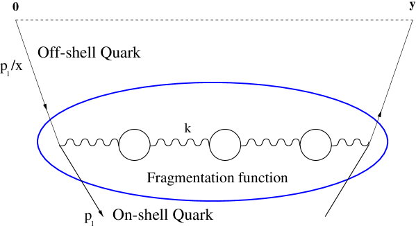
Figure 3: The diagram contributing to $\tilde{D}(N,m^{2})$ in the light-cone axial gauge $A\cdot y=0$ and in the large $N_{f}$ limit.

The ${\cal O}(\alpha_{s})$ result for an off-shell gluon emission derived in the previous section can be promoted to a single dressed gluon (SDG) renormalon sum by integrating over the gluon virtuality $k^{2}$, with the coupling being renormalized at $k^{2}$ (see fig. 3). It is convenient to define a factorization scheme and scale invariant quantity, by taking the logarithmic derivative with respect to $m^{2}$. Contrary to the fragmentation function itself, its logarithmic derivative is free of ultraviolet divergence. The result, written in moment space (4) as a scheme invariant Borel transform [30], is

$$\frac{d\tilde{D}_{\hbox{\tiny SDG}}(N,m^{2})}{d\ln m^{2}}=\frac{C_{F}}{\beta_{0}}\,\int_{0}^{\infty}du\,\,T(u)\,{\left(m^{2}/\Lambda^{2}\right)}^{-u}\,\int_{0}^{1}\,dx\,\left(x^{N-1}-1\right)\,B_{D}(u,x),$$ (30)

where $x^{N-1}$ has been replaced by $x^{N-1}-1$ to account for virtual corrections, and

$$B_{D}(u,x)=\frac{-u\sin\pi u}{2\pi}\,{\rm e}^{cu}\,m^{2u}\,$$

$$\int_{0}^{\infty}\frac{dk^{2}}{k^{2(1+u)}}\,\left[\frac{1+x^{2}}{1-x}\,\ln{\left(x\,(k^{2}/m^{2})+(1-x)^{2}\right)}\,+\,x(1-x)\,\frac{2+(k^{2}/m^{2})}{{x\,(k^{2}/m^{2})+(1-x)^{2}}}\right].$$

Note that in (3.2.2) $m^{2}$ can be scaled out, so $B_{D}(u,x)$ is independent of any scale and the dependence of ${d\ln\tilde{D}_{\hbox{\tiny SDG}}(N,m^{2})}/{d\ln m^{2}}$ on $m^{2}$ appears only through ${\left(m^{2}/\Lambda^{2}\right)}^{-u}$. Here the factor $(-u)$ is associated with the logarithmic derivative, the sine appears upon taking the time-like discontinuity of the dressed gluon propagator, and $T(u)$ is defined as the Laplace transform of the coupling

$$A(k^{2})=\beta_{0}{\alpha}_{s}(k^{2})/\pi=\int_{0}^{\infty}\,du\,T(u)\left(k^{2}/\Lambda^{2}\right)^{-u}.$$ (32)

$T(u)$ depends only on the coefficients of the renormalization group equation of $\alpha_{s}/\pi$. For a one-loop running coupling $T(u)=1$ and in the two-loop case

$$T(u)=(u\delta)^{u\delta}\exp(-u\delta)/\Gamma(1+u\delta),$$ (33)

where $\delta\equiv\beta_{1}/\beta_{0}^{2}$, with $\beta_{0}=\pi b_{0}$ and $\beta_{1}=\pi^{2}b_{1}$ as defined in Eq. (28) of [13]. Defining $\Lambda$ in the ${\overline{\rm MS}}$ scheme,

$$c=5/3+{\cal O}(1/\beta_{0}).$$ (34)

Performing the integration over the gluon virtuality in (3.2.2) we get

$$B_{D}(u,x)=-\,{\rm e}^{cu}\,\left(\frac{x}{(1-x)^{2}}\right)^{u}\,\left[\frac{x}{1-x}\,(1-u)+\frac{1}{2}(1-x)\,(1+u)\right].$$ (35)

Here we used integrals of the form

$$\int_{0}^{\infty}\frac{dy}{y^{1+u}}\,\frac{1}{y+(1-x)^{2}}=-\frac{\pi}{\sin\pi u}\,(1-x)^{-2(1+u)}$$

with $y=xk^{2}/m^{2}$. Note that this $\sin\pi u$ factor in the denominator cancels against the one in the numerator of (3.2.2), so there are no renormalon singularities in (35). There is however, a convergence constraint for the Borel integral (30) at $u\longrightarrow\infty$. In the case of one-loop running coupling ($T(u)=1$) the constraint is:

$$m^{2}(1-x)^{2}/x>\Lambda^{2}\exp(c).$$ (36)

As we will see below, this singular behavior for $x\longrightarrow 1$ translates into renormalons upon performing the $x$ integration.

Note also the appearance of the factor $(1-u)$ in front of the $x\longrightarrow 1$ singular term in (35). This reflects a relation between the two terms in the squared matrix element (21). Let us examine the two corresponding terms in the square brackets in (3.2.2): the first is the source of the $1$ and the second, which can be represented as a logarithmic derivative of the first with respect to $k^{2}$, yields the $-u$. As we will see, in moment space this structure leads to the absence of a renormalon singularity at $u=1$, while renormalons do appear at all other integer and half integer values.

Let us perform now the integration over $x$ in Eq. (30). We obtain

$$\frac{d\ln\tilde{D}_{\hbox{\tiny SDG}}(N,m^{2})}{d\ln m^{2}}=\frac{C_{F}}{\beta_{0}}\,\int_{0}^{\infty}du\,\,T(u)\,{\left(m^{2}/\Lambda^{2}\right)}^{-u}\,B_{\tilde{D}}(u,N),$$ (37)

with

$$B_{\tilde{D}}(u,N) = \,\int_{0}^{1}\,dx\,\left(x^{N-1}-1\right)\,B_{D}(u,x)=$$ (38)

$$-{\rm e}^{cu}\,\left[(1-u)\Gamma(-2u)\left(\frac{\Gamma(N+1+u)}{\Gamma(N+1-u)}-\frac{\Gamma(2+u)}{\Gamma(2-u)}\right)\right.$$

$$\hskip 50.0pt\left.+\frac{1}{2}(1+u)\Gamma(2-2u)\left(\frac{\Gamma(N+u)}{\Gamma(N+2-u)}-\frac{\Gamma(1+u)}{\Gamma(3-u)}\right)\right].$$

As anticipated, $B_{\tilde{D}}(u,N)$ has infrared renormalon singularities (simple poles) at all positive integer and half integer values of $u$, with the single exception of $u=1$.

3.2.3 Ultraviolet subtraction for the fragmentation function

In order to obtain the fragmentation function itself Eq. (37) needs to be integrated. The integration involves a subtraction of the ultraviolet divergent contribution, as standardly done in collinear factorization. The result takes the form:

$$\tilde{D}_{\hbox{\tiny SDG}}(N,m^{2};\mu^{2})\,=\,1\,+$$

$$\,\frac{C_{F}}{\beta_{0}}\,\int_{0}^{\infty}\,du\,T(u)\,\left(m^{2}/{\Lambda}^{2}\right)^{-u}\,\left[-\frac{B_{\tilde{D}}(u,N)}{u}\,+\,\left(\mu^{2}/m^{2}\right)^{-u}\,\frac{B_{\tilde{E}}(u,N)}{u}\right],$$ (39)

where $\mu$ is a factorization scale and $B_{\tilde{E}}(u,N)$ is the Altarelli-Parisi evolution kernel (the subscript $E$ stands for Evolution),

$$B_{\tilde{E}}(u,N)\,=\,\sum_{n=0}^{\infty}\frac{\gamma_{n}(N)\,u^{n}}{n!}.$$ (40)

This subtraction guarantees the existence of the integral near $u=0$ by canceling the $1/u$ singularity.

We stress that this subtraction is required only because we calculate the fragmentation process alone. In any infrared and collinear safe observable the coefficient function will compensate the $1/u$ singularity. This is demonstrated in Sec. 4 in the case of the differential cross section in $e^{+}e^{-}$ annihilation. Through the evolution term the fragmentation function becomes factorization-scheme and scale dependent although the full result for the cross section is not.

The leading order coefficient in (40) is renormalization-scheme invariant, and it equals to the $u=0$ limit of (38), ensuring the cancellation of the $1/u$ singularity in (3.2.3),

$$\gamma_{0}(N)=S_{1}(N)-\frac{3}{4}+\frac{1}{2}\left(\frac{1}{N+1}-\frac{1}{N}\right),$$

where $S_{k}(N)\equiv\sum_{j=1}^{N}{1}/{j^{k}}$, so that $S_{1}(N)=\Psi(N+1)+\gamma_{E}$. In the $\overline{\rm MS}$ factorization scheme $\gamma_{n}(N)$ are known to two-loop order ($n=1$) in full [31] and to all orders in the large-$\beta_{0}$ limit [32]. The latter is given by

$$\tilde{E}(N,A) = \sum_{n=0}^{\infty}\gamma_{n}(N)A^{n+1}={\cal A}\,\bigg{[}\Psi(N+A)-\Psi(1+A)$$

$$+ \frac{N-1}{2}\left(\frac{A^{2}+2A-1}{1+A}\,\frac{1}{N+A}-\frac{(1+A)^{2}}{2+A}\frac{1}{N+1+A}\right)\bigg{]}\,+\,{\cal O}(1/\beta_{0})$$

with

$${\cal A}=\frac{\sin\pi A}{\pi}\,\,\frac{\Gamma(4+2A)}{6\Gamma(2+A)^{2}}\,+\,{\cal O}(1/\beta_{0}).$$ (42)

${\cal A}$ is the all-order large-$\beta_{0}$ expression in $\overline{\rm MS}$ for the gluon bremsstrahlung effective charge [33] or the cusp anomalous dimension [34, 35, 36], and $A=\beta_{0}\alpha_{s}/\pi$ is the large-$\beta_{0}$ coupling in $\overline{\rm MS}$.

Using eqs. (38) through (3.2.3) it is straightforward to extract the large-$\beta_{0}$ coefficients of the heavy-quark fragmentation function $\tilde{D}(N,m^{2})$ in the $\overline{\rm MS}$ factorization scheme to all orders, for example

$$\tilde{D}_{\hbox{\tiny SDG}}(N,m^{2})\,\,=\,1\,+\frac{C_{F}}{\beta_{0}}\left\{\bigg{[}-S_{1}^{2}(N)+\right.$$

$$\left(\frac{1}{N}-\frac{1}{N+1}+1\right)S_{1}(N)+1-S_{2}(N)+\frac{1}{2(N+1)}-\frac{1}{2N}-\frac{1}{(N+1)^{2}}\bigg{]}A(m^{2})\,+$$

$$\hskip 5.0pt\bigg{[}-\frac{2}{3}S_{1}^{3}(N)+\left(\frac{1}{N}-\frac{1}{N+1}-\frac{2}{3}\right)S_{1}^{2}(N)$$

$$+\left(\frac{1}{9}-\frac{\pi^{2}}{3}+\frac{8}{3}\frac{1}{N}-\frac{8}{3}\frac{1}{N+1}-\frac{1}{(N+1)^{2}}-\frac{1}{N^{2}}\right)S_{1}(N)$$

$$\hskip 5.0pt-\frac{5}{6}S_{2}(N)+\frac{1}{6}S_{3}(N)+\left(\frac{1}{4}-\frac{1}{6}\frac{1}{N+1}+\frac{1}{6}\frac{1}{N}\right)\pi^{2}+\frac{173}{96}+\frac{19}{36}\frac{1}{N}-\frac{19}{36}\frac{1}{N+1}$$

$$\hskip 5.0pt\left.-\frac{5}{12}\frac{1}{N^{2}}-\frac{9}{4}\frac{1}{(N+1)^{2}}+\frac{1}{4}\frac{1}{N^{3}}-\frac{1}{4}\frac{1}{(N+1)^{3}}\bigg{]}{A(m^{2})}^{2}\,+\,{\cal O}({A(m^{2})}^{3})\right\}\;.$$ (43)

The order $\alpha_{s}$ result is known. It was extracted by Mele and Nason [8], starting from the single inclusive cross section for heavy-quark production in $e^{+}e^{-}$ annihilation and subtracting the coefficient function for the massless case. More recently, this term has been computed in a process-independent way in [13]. Our calculation extends it to all orders in the large-$\beta_{0}$ limit.

In addition to the resummation of large perturbative corrections, the all-order large-$\beta_{0}$ result can be used to extract some non-perturbative information on the fragmentation process. As we saw, in the large-$\beta_{0}$ limit renormalons appear always as simple poles, and are exclusively associated with the integration over $x$. It should be noted that the subtracted term (Eq. (40)) has no infrared renormalons in factorization schemes such as ${\overline{\rm MS}}$.

In (38) the first singularity is located at $u=1/2$ and it corresponds to ${\cal O}(\Lambda/m)$ corrections. The second singularity is at $u=3/2$ (${\cal O}(\Lambda^{3}/m^{3})$ corrections) and higher singularities appear at all integers and half integers on the positive Borel axis. It is particularly interesting to note the absence of the renormalon at $u=1$. As explained above this structure can be traced back to the relation between the single and the double pole terms in $2p_{1}k+k^{2}$ in the squared matrix element (21).

Both the presence on the renormalon singularity at $u=1/2$ and the absence of the one at $u=1$ are consistent with the findings of Nason and Webber [15], which considered the large-$N$ limit of the fragmentation function in $e^{+}e^{-}$ annihilation. We confirm these conclusions in a more general, process independent context (and for a generic $N$), and derive an expression for the Borel function allowing to combine resummation with parametrization of power corrections. It is not known, and certainly deserves further investigation, whether a renormalon at $u=1$ does appear in the full theory.

3.2.4 The large-$x$ region and the Sudakov exponent in perturbation theory and beyond

At large $x$ multiple emission plays an important rôle. The SDG result can be readily used to derive the exponentiation kernel in the approximation of independent emission. Extracting the log-enhanced terms from (38) and (40) one gets

$$\!\!\!\!\!\left.\ln\tilde{D}(N,m^{2})\right|_{\hbox{\tiny DGE}}=\frac{C_{F}}{\beta_{0}}\,\int_{0}^{\infty}\,du\left[-\frac{B_{\tilde{D}}^{\hbox{\tiny DGE}}(u,N)}{u}\,\,+\,\frac{\,B_{\cal A}(u)}{u}\,\ln N\right]\,\,T(u)\,\left(m^{2}/{\Lambda}^{2}\right)^{-u}$$ (44)

where $\mu$ was set equal to $m$,

$$B_{\tilde{D}}^{\hbox{\tiny DGE}}(u,N)=-\,{\rm e}^{cu}\,(1-u)\,\Gamma(-2u)\,\left[N^{2u}-1\right]\,+\,{\cal O}(1/\beta_{0}),$$ (45)

and $B_{\cal A}(u)=1+c\frac{u}{1!}+\ldots$ is the Borel transform of the cusp anomalous dimension (42).

Note that we write here a perturbative expansion for $\ln\tilde{D}(N,m^{2})$. This is not just a formal manipulation which holds to order $\alpha_{s}$, but rather a statement about the structure of higher-order terms. The logarithmically enhanced terms, as opposed to the expressions in (37), (3.2.3) and (3.2.3), exponentiate: they can be written to all orders as

$$\tilde{D}(N,m^{2})=\exp\left\{\sum_{n=0}^{\infty}\sum_{k=1}^{n+1}d_{n,k}\,\alpha_{s}^{n}\ln^{k}N\right\}.$$

Although (44) was derived strictly in the large $\beta_{0}$ limit, i.e. leading-log (LL) accuracy, it can be generalized in a straightforward way to comply with NLL accuracy in the full theory [33, 18, 29] by using the two-loop running coupling (33) and replacing $c$ of Eq. (34) in the exponent ${\rm e}^{cu}$ and in $B_{\cal A}(u)$ by

$$c\,\longrightarrow\,a_{2}=5/3+(1/3-\pi^{2}/12)C_{A}/\beta_{0}.$$ (46)

It should be noted, though, that the functional form of the Borel transform is not known beyond the large-$\beta_{0}$ limit, so the replacement of $c$ by $a_{2}$ in (45) is not proven. As discussed in a similar context in [20] the same logarithmic accuracy can be achieved in different ways, e.g. by replacing the factor ${\rm e}^{(5/3)u}$ in (45) by ${\rm e}^{(5/3)u}(1+u(a_{2}-5/3))$. We will assume here the simple replacement (46).

The renormalon structure of the Sudakov exponent, is similar to that of the full SDG result (38): the leading renormalon is at $u=1/2$ and subleading ones appear at all integer and half integers $u\geq 3/2$. In accordance with the general property of the fragmentation function (Sec. 2) these corrections show up in (44) on the scale $m/N$. The appearance of these powers corrections in the exponent leads to factorization, in moment space, of the non-perturbative contribution to the fragmentation function. Moreover, it also implies that these corrections exponentiate together with the perturbative logs.

Based on the result of Sec. 2 we can further deduce that in the full theory, as in (44), renormalons in the Sudakov exponent appear as single poles, involving no anomalous dimension. In case on non-vanishing anomalous dimensions $\gamma_{i}$, power corrections are modified by logarithms, $(\mu N/m)^{i}(\ln\mu/m)^{\gamma_{i}/(2\beta_{0})}$ where $\mu$ is a cutoff. This behavior contradicts Eq. (10) and therefore the anomalous dimensions must vanish.

We conclude that non-perturbative corrections to the heavy-quark fragmentation process appear as

$$\tilde{D}(N,m^{2})=\tilde{D}_{\hbox{\tiny PT}}(N,m^{2})\,\tilde{D}_{\hbox{\tiny NP}}(N\Lambda/m),$$ (47)

where $\tilde{D}_{\hbox{\tiny PT}}(N,m^{2})$ is obtained by exponentiating the (regularized) renormalons sum (44) and

$$\tilde{D}_{\hbox{\tiny NP}}(N\Lambda/m)=\exp\left\{-\omega_{1}\frac{C_{F}}{\beta_{0}}\frac{N\Lambda}{m}-\omega_{3}\frac{C_{F}}{\beta_{0}}\left(\frac{N\Lambda}{m}\right)^{3}-\omega_{4}\frac{C_{F}}{\beta_{0}}\left(\frac{N\Lambda}{m}\right)^{4}+\cdots\right\},$$ (48)

which is characterized by the absence of the second power of $(N\Lambda/m)$. Here $\omega_{n}$ are left as free parameters. These parameters are defined only within a given regularization prescription for the renormalons, corresponding to a definite separation between the perturbative and non-perturbative components in $\tilde{D}(N,m^{2})$. A physically meaningful separation would be the one based on a momentum cutoff, or, alternatively, a principle-value regularization of the Borel sum, which can be readily related to a cutoff [17]. Having performed the renormalon sum in $\tilde{D}_{\hbox{\tiny PT}}(N,m^{2})$, the parameters in $\tilde{D}_{\hbox{\tiny NP}}(N\Lambda/m)$ can be fixed by comparison with experimental data.

Going over to $x$ space, the product in (47) becomes a convolution with a shape function depending on $m(1-x)$. As discussed in the context of event-shape distributions in $e^{+}e^{-}$ annihilation [37, 21, 24, 18], this convolution generates a shift of the perturbative distribution proportional to $\omega_{1}$ and a deformation of its shape by $\omega_{3}$ and on.

It should be stressed that both the resummation formula (44) and the non-perturbative corrections in (48) are expected to dominate only for $N\gg 1$. The first few moments are surely affected by perturbative and non-perturbative contributions on the scale $m$ (as opposed to $m/N$), which do not necessarily exponentiate and were neglected here. The phenomenological implications of (44) and (48) will be discussed in more detail in the context of $e^{+}e^{-}$ annihilation.

4 Heavy meson production in $e^{+}e^{-}$ annihilation

4.1 Calculation of the Sudakov exponent

Let us consider now the specific process of heavy-flavor production in $e^{+}e^{-}$ annihilation. To be concrete, let us concentrate on the vector current contribution to the process $e^{+}e^{-}\longrightarrow Q\bar{Q}g$ where the momentum of the virtual photon is $q$ (the centre-of-mass energy is $\sqrt{q^{2}}$), and the quarks have momenta $p_{1}$ and $p_{2}$, energy fractions $x\equiv 2p_{1}q/q^{2}$ and $\bar{x}\equiv 2p_{2}q/q^{2}$ and masses $p_{1}^{2}=p_{2}^{2}=m^{2}\equiv\rho\,q^{2}/4$.

As in [15] we begin with the exact matrix element with an off-shell gluon, $k^{2}\equiv\epsilon q^{2}$. The result for the cross section is,

$$\frac{1}{\sigma}\frac{d\sigma}{dx\,d{\bar{x}}} = \frac{C_{F}\alpha_{s}}{2\pi}\,\frac{1}{\sqrt{1-\rho}}\left[\frac{(x+\epsilon+\rho/2)^{2}+({\bar{x}}+\epsilon+\rho/2)^{2}-2\rho(1+\epsilon+\rho/2)}{(1+\rho/2)(1-x)(1-\bar{x})}\right.$$ (49)

$$\left.-\frac{\epsilon+\rho/2}{(1-x)^{2}}-\frac{\epsilon+\rho/2}{(1-\bar{x})^{2}}\right].$$

It is straightforward to verify that when taking the quasi-collinear limit this expression reduces to the approximate one we calculated in the previous section in a process-independent way. Note first that the propagator which becomes singular in this limit is inversely proportional to $2p_{1}k+k^{2}=q^{2}-2p_{2}q=q^{2}(1-\bar{x})$, where we used momentum conservation: $k=q-p_{1}-p_{2}$. As follows from Eq. (20), the quasi-collinear limit is the one in which $1-\bar{x}$, $\epsilon$ and $\rho$ (and $k_{\perp}^{2}/q^{2}$) all become small but the ratios between them are fixed. In this limit the leading contribution to (49) takes the form:

$$\frac{1}{\sigma}\frac{d\sigma}{dx\,d{\bar{x}}}\simeq\frac{C_{F}\alpha_{s}}{2\pi}\,\left[\frac{1+x^{2}}{1-x}\frac{1}{(1-\bar{x})}-\frac{\rho/2+\epsilon}{(1-\bar{x})^{2}}\right],$$ (50)

which fully agrees with (21).

Owing to the non-vanishing quark mass and to its inclusive nature, the differential cross section $d\sigma/dx$ is an infrared and collinear safe quantity. It can therefore be calculated in perturbation theory to any order, with no need to perform factorization.

Here we perform such a calculation having in mind the experimentally interesting scenario with $\rho\ll 1$ as well as $1-x\ll 1$ (or $N\gg 1$). These conditions are easily met for charm and bottom production at LEP1 energies, i.e. $q\simeq 91~{}{\rm GeV}$. In this limit logarithmically enhanced terms of either $\rho$ or $N$ need to be resummed. At the same time, in order to address the issue of power corrections, we must perform renormalon resummation. This calls for DGE.

In this section we perform the calculation by integrating the full off-shell gluon matrix element (49) over the exact phase space. This calculation follows the steps of the first derivation of the DGE result for the thrust distribution [18], based on the characteristic function of [38]: It proceeds by identifying log-enhanced terms and deriving a Borel representation which generates these terms to all orders in the large-$\beta_{0}$ limit. Finally, this Borel sum is used as the exponentiation kernel.

First we integrate (49) over $\bar{x}$, getting a characteristic function. The limits of phase space (see [15]) are:

$$\bar{x}_{\max/\min} = \frac{(2-x)(1-x-\epsilon+\rho/2)\pm\Xi}{2(1-x)+\rho/2}$$

$$\Xi = \sqrt{x^{2}-\rho}\sqrt{(1-x-\epsilon)^{2}-\epsilon\rho}.$$ (52)

As Fig. 4 shows, for a given $\rho$ the phase-space shrinks as $\epsilon$ increases. Note that even with a vanishing gluon virtuality the phase-space boundary does not reach the line $\bar{x}=1$ (with the exception of a point at $x=1$), where the matrix element is singular. Consequently the differential cross section $d\sigma/dx$ is infrared and collinear safe.

Figure 4: $QQg$ phase-space boundaries in the $x$–$\bar{x}$ plane, with varying gluon virtualities $\epsilon=(1-\sqrt{\rho})^{2}\,i/10$, for $i=0$ through $9$, with $\rho=0.04$.

The resulting characteristic function is:

$$\frac{1}{\sigma}\frac{d\sigma}{dx}(\epsilon,x,\rho)=\frac{C_{F}\alpha_{s}}{\pi}\left[{\cal F}_{1}+{\cal F}_{2}+{\cal F}_{3}\right]$$ (53)

with

$${\cal F}_{1} = \frac{-(\rho+2\epsilon)}{\rho\xi^{2}+4\epsilon-4\epsilon\xi+4\epsilon^{2}-4\epsilon\rho}\,\Xi\,$$

$${\cal F}_{2} = \frac{4-4\xi+2\xi^{2}+8\epsilon-4\epsilon\xi-2\rho\xi+4\epsilon^{2}-\rho^{2}}{2\xi(2+\rho)}\,\ln\left(\frac{2\xi+2\epsilon-2\xi^{2}+2\epsilon\xi-\rho\xi+2\,\Xi}{{2\xi+2\epsilon-2\xi^{2}+2\epsilon\xi-\rho\xi-2\,\Xi}}\right)$$

$${\cal F}_{3} = \left(\frac{24\epsilon}{\xi(2+\rho)\rho^{2}}-\frac{\rho+2\epsilon}{\rho\xi^{2}}-\frac{2(\rho^{2}+48\epsilon)}{(2+\rho)\rho^{2}(4\xi+\rho)}+\frac{2(-4+\rho)(-\rho+4\epsilon)}{(2+\rho)\rho(4\xi+\rho)^{2}}\right)\,\Xi,$$ (54)

where $\xi\equiv 1-x$. These three terms are distinguished by the singularity of the corresponding term in the matrix element at $\bar{x}\longrightarrow 1$: ${\cal F}_{1}$ originates in a double pole, ${\cal F}_{2}$ in a single pole and ${\cal F}_{3}$ in non-singular terms.

Next we perform the integral over the gluon virtuality $\epsilon$ in the range $0<\epsilon<\epsilon_{\max}$, where the upper integration limit,

$$\epsilon_{\max}=\frac{1}{4}\,\left[\sqrt{\rho}-\sqrt{\rho+4(1-x)}\right]^{2}$$ (55)

is the point where $\Xi=0$ and $\bar{x}_{\min}=\bar{x}_{\max}$. The Borel function is obtained by computing:

$$B(u,x,\rho)=-\frac{\sin\pi u}{\pi u}\,{\rm e}^{cu}\,\,I(u,x,\rho),\quad\quad I(u,x,\rho)\equiv u\,\int_{0}^{\epsilon_{\max}}d\epsilon\,\epsilon^{-1-u}\,{\cal F}(\epsilon,x,\rho).$$ (56)

The exact integration is complicated. The full result can only be written in terms of hypergeometric functions. However, in the following we will not need the full result, as we are interested in the logarithmically enhanced terms alone. Assuming the hierarchy $\rho\ll\xi\ll 1$ the leading terms in the Borel function are rather simple. The integrals corresponding to the three terms in the characteristic functions are the following:

$$I_{1} \simeq \,\frac{\pi u}{\sin\pi u}\,\xi^{-1-2u}(\rho/4)^{-u},$$

$$I_{2} \simeq \frac{1}{u}\,\xi^{-1-u}\,-\,\frac{\pi}{\sin\pi u}\,\xi^{-1-2u}(\rho/4)^{-u}$$

$$I_{3} \simeq \frac{1}{2}\xi^{-1-u}\,\left[\frac{1}{1-u}+\frac{1}{2-u}\right]$$ (57)

where we neglected terms suppressed by powers of either $\xi$ or $\rho$. The Borel function which generates all the log-enhanced terms in the large $\beta_{0}$ limit is therefore given by

$$B(u,x=1-\xi,\rho) = \frac{{\rm e}^{cu}}{\xi}\,\bigg{\{}\frac{1}{u}\,(1-u)\,\left(\rho/4\right)^{-u}\,\xi^{-2u}$$ (58)

$$\hskip 40.0pt-\,\frac{\sin\pi u}{2\pi u}\left(\frac{2}{u}+\frac{1}{1-u}+\frac{1}{2-u}\right)\,\,\xi^{-u}\bigg{\}}.$$

Finally we perform the $x$ integration and incorporate virtual corrections through the subtraction of the result at $N=1$. In spite of the fact that (58) was derived assuming the hierarchy $\rho\ll\xi\ll 1$, it is sufficient to get the exact result for the Sudakov exponent, since the region of $\xi\mathrel{\mathchoice{\vbox{\offinterlineskip\halign{$\m@th\displaystyle\hfil#\hfil$\cr<\crcr\sim\crcr} }}{\vbox{\offinterlineskip\halign{$\m@th\textstyle\hfil#\hfil$\cr<\crcr\sim\crcr} }}{\vbox{\offinterlineskip\halign{$\m@th\scriptstyle\hfil#\hfil$\cr<\crcr\sim\crcr} }}{\vbox{\offinterlineskip\halign{$\m@th\scriptscriptstyle\hfil#\hfil$\cr<\crcr\sim\crcr} }}}\rho$ yields contributions which are suppressed by powers of $\rho$. The resulting Borel representation of the Sudakov exponent is

$$\left.\ln\tilde{\sigma}(N,q^{2},m^{2})\right|_{\hbox{\tiny DGE}}=\frac{C_{F}}{\beta_{0}}\,\int_{0}^{\infty}\,duB_{\sigma}(u,N,m^{2}/q^{2})\,\,T(u)\,\exp(-u\ln q^{2}/{\Lambda}^{2})$$ (59)

with

$$B_{\sigma}(u,N,m^{2}/q^{2}) = {\rm e}^{cu}\,\bigg{\{}\frac{1}{u}\,(1-u)\,\Gamma(-2u)\,\left[N^{2u}-1\right]\,\left({m^{2}}/{q^{2}}\right)^{-u}$$ (60)

$$\hskip 30.0pt-\frac{\sin\pi u}{2\pi u}\left(\frac{2}{u}+\frac{1}{1-u}+\frac{1}{2-u}\right)\,\Gamma(-u)\,\left[N^{u}-1\right]\bigg{\}}.$$

4.2 Factorization

Our result (59) for the Sudakov exponent of the $e^{+}e^{-}\longrightarrow Q+X$ differential cross section involves two external scales, $q^{2}$ and $m^{2}$. Therefore, in addition to Sudakov logs $L\equiv\ln N$, it contains collinear logs $l\equiv\ln q^{2}/m^{2}$. The latter can be seen a reflection of evolution from the scale $m^{2}$ at which the fragmentation process of the heavy quark takes place (Sec. 2 and 3) to the $e^{+}e^{-}$ centre-of-mass energy squared $q^{2}$ at which the hard interaction takes place. The contributions to the cross section from these two subprocesses can be written separately by introducing some factorization procedure. Since Sudakov logs emerge from both subprocesses, this separation will be useful to distinguish between them.

Factorization takes the form of a product in moment space, so the Sudakov exponent can be written as a sum of the following three exponents,

$$\left.\ln\tilde{\sigma}(N,q^{2},m^{2})\right|_{\hbox{\tiny DGE}}=\,\left.\ln\tilde{J}(N,q^{2})\right|_{\hbox{\tiny DGE}}\,+\,\left.\ln\tilde{E}(N,q^{2},m^{2})\right|_{\hbox{\tiny DGE}}\,+\left.\ln\tilde{D}(N,m^{2})\right|_{\hbox{\tiny DGE}}\,$$ (61)

where $\ln\tilde{D}(N,m^{2})$ corresponds to Eq. (44), i.e. the (process independent) heavy-quark fragmentation depending on the scale $m^{2}$, $\ln\tilde{J}(N,q^{2})$ corresponds to the $e^{+}e^{-}$ coefficient function depending on the scale $q^{2}$, and $\ln\tilde{E}(N,q^{2},m^{2})$ represents the evolution between these two scales and thus it depends on both.

Performing factorization, the Sudakov exponent corresponding to the fragmentation subprocess is (44), the evolution is given by

$$\!\!\left.\ln\tilde{E}(N,q^{2},m^{2})\right|_{\hbox{\tiny DGE}}=\frac{C_{F}}{\beta_{0}}\,\int_{0}^{\infty}du\,\,T(u)\,\left(q^{2}/{\Lambda}^{2}\right)^{-u}\,\frac{B_{\cal A}(u)}{u}\,\ln N\,\left\{1\,-\,\left({m^{2}}/{q^{2}}\right)^{-u}\right\}\,$$ (62)

and the Sudakov exponent of the $e^{+}e^{-}$ coefficient function is

$$\left.\ln\tilde{J}(N,q^{2})\right|_{\hbox{\tiny DGE}}= -\frac{C_{F}}{\beta_{0}}\,\int_{0}^{\infty}\,du\,T(u)\,\left(q^{2}/{\Lambda}^{2}\right)^{-u}\,$$

$$\bigg{\{}{\rm e}^{cu}\,\frac{\sin\pi u}{2\pi u}\left(\frac{2}{u}+\frac{1}{1-u}+\frac{1}{2-u}\right)\,\Gamma(-u)\,\left[N^{u}-1\right]\,+\,\frac{B_{\cal A}(u)}{u}\,\ln N\bigg{\}}.\,$$

The essential ingredient in obtaining a factorized formula is that each of the three exponents corresponding to the separate subprocesses has a well-defined perturbative expansion: there are no $1/u$ singularities in these Borel functions. Of course, there is some arbitrariness in this procedure as far as higher-order terms are concerned. Here we chose the natural factorization scales as the external scales, $m^{2}$ and $q^{2}$. The subtracted term $B_{\cal A}(u)=1+a_{2}u+\ldots$ depends on the factorization scheme. In ${\overline{\rm MS}}$, the coefficient $a_{2}$ is given by (46). Owing to the fact that the expressions above correspond to all-order resummation, factorization-scale and scheme dependent terms cancel out completely in the sum (61). Of course, if any of the three exponents is replaced by some fixed order or a fixed-logarithmic accuracy approximation, some factorization-scale and scheme dependence will appear in the final result for the cross section.

Note that while $\tilde{J}(N,q^{2})$ and $\tilde{D}(N,m^{2})$ contain Sudakov double logs (upon expanding the exponent, the highest power of $\ln N$ is twice that of the coupling at each order), the evolution factor $\tilde{E}(N,q^{2},m^{2})$ contains at most $\ln N$ to the same power as the coupling. This is so because $\ln\tilde{E}(N,q^{2},m^{2})$ has just one power of $\ln N$ to any order in $\alpha_{s}$ [39, 40, 35].

Having performed factorization we can compare the results obtained for the two subprocesses (44) and (4.2) to the corresponding process-independent calculations. The DGE Sudakov exponent for the heavy-quark fragmentation subprocess has been identified with the result obtained in the process-independent calculation (44). It follows that the only scale which plays a rôle in the fragmentation process $\tilde{D}(N,m^{2})$ at large $N$ is $m/N$. As shown in Sec. 2, this is a general property of the fragmentation function which holds beyond the perturbative level.

Similarly, the DGE Sudakov exponent for the $e^{+}e^{-}$ coefficient function (4.2) can be identified as the one appearing in a massless quark fragmentation process which was calculated in [29]. The same all-order result was obtained [29, 23, 20] for the $F_{2}$ structure function at large $N$. As discussed in [29, 23], $\left.\ln\tilde{J}(N,q^{2})\right|_{\hbox{\tiny DGE}}$ is associated with radiation from the undetected quark (or the outgoing quark in a deep-inelastic process at large $x_{\rm Bj}$) and the formation of a jet (this explains the notation $\tilde{J}$) with invariant mass $q^{2}/N$, which recoils against the detected quark. This identification means, in particular, that $\left.\ln\tilde{J}(N,q^{2})\right|_{\hbox{\tiny DGE}}$ is not specific to the particular process in which two heavy quarks are produced: it would be the same if the recoiling jet would have been formed around a light quark. The internal structure of the jet is not resolved as the relevant scale is its invariant mass.

The fully factorized process of heavy-quark production in $e^{+}e^{-}$ annihilation is shown in Fig. 5. The hard blob represents radiative corrections with virtualities of order of the centre-of-mass energy squared $q^{2}$. The detected heavy meson ($p_{1}$) emerges from the lower jet in the figure. Although a priori two-jet production is symmetric, the fact that one measures a single particle inclusive cross section breaks the symmetry: the measurement is sensitive to different features of the two jets. The fragmentation blob represents $\tilde{D}(N,m^{2})$. It accounts for soft and collinear radiation on the scale $m/N$. The recoiling jet on the upper part of the figure represents $\tilde{J}(N,q^{2})$, accounting for soft and collinear radiation of the scale $q^{2}/N$. The soft blob is associated with the evolution factor $\tilde{E}(N,q^{2},m^{2})$. It accounts for gluons whose momentum components are all small. These gluons interact with eikonalized quarks: They are insensitive to the invariant mass or the structure of either of the two jets.

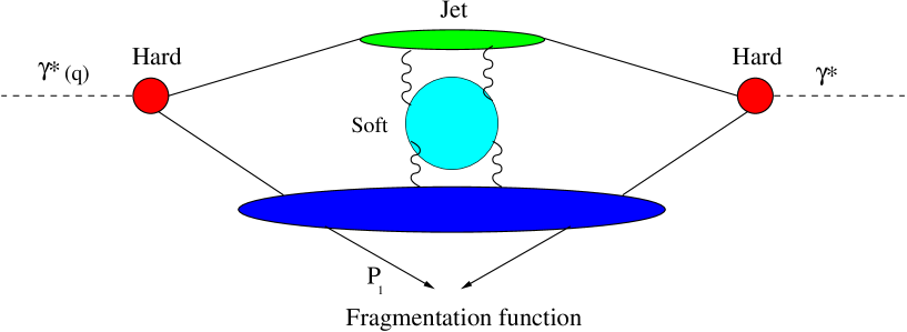
Figure 5: Factorization of the process $\gamma^{*}\longrightarrow Q+X$ at large $N$.

Alongside the dominant perturbative corrections which are summarized by (61), the large-$N$ limit singles out certain non-perturbative corrections. Such corrections appear in two of the subprocesses described above: in $\tilde{D}(N,m^{2})$ they appear on the scale $m/N$ and in $\tilde{J}(N,q^{2})$ on the scale $q^{2}/N$. The evolution factor $\tilde{E}(N,q^{2},m^{2})$, on the other hand, has no power corrections. The presence of power corrections, as well as their parametric form, can be deduced from the renormalon singularities in the corresponding Borel sums. In both $\tilde{D}(N,m^{2})$ and $\tilde{J}(N,q^{2})$, the dominant corrections at large $N$ appear in the Sudakov exponents, Eq. (44) and (4.2), so these power corrections exponentiate together with the perturbative logs. The renormalon singularities of $\left.\ln\tilde{J}(N,q^{2})\right|_{\hbox{\tiny DGE}}$ were analyzed in [29, 23, 20]. They lead to $\Lambda^{2}N/q^{2}$ and $\Lambda^{4}N^{2}/q^{4}$ corrections at the exponent, as summarized by Eq. (50) in [29]. As discussed in the previous section the renormalon singularities of the heavy-quark fragmentation exponent $\left.\ln\tilde{D}(N,m^{2})\right|_{\hbox{\tiny DGE}}$ appear at $u=1/2$ and at any integer and half integer such that $u\geq 3/2$. There is no renormalon pole at $u=1$ owing to the factor $(1-u)$ in (45).

5 Implications for phenomenology

In the previous sections we studied the problem of heavy-quark fragmentation, concentrating on the large-$N$ limit. We began by identifying the formal limit in which simplification occurs, namely where $N$ and $m$ get large simultaneously with the ratio $m/N$ fixed. We then performed a process-independent perturbative calculation by DGE, facilitating the resummation of Sudakov logs as well as that of running-coupling effects. The combined treatment of Sudakov logs and renormalons sets the basis for a systematic parametrization of power-suppressed corrections on the scale $m/N$, which exponentiate together with the perturbative logs. Then, specializing to the case of $e^{+}e^{-}$ annihilation, we demonstrated how this result for the Sudakov exponent of the fragmentation function emerges from the process-specific renormalon calculation upon factorization. The Sudakov-resummed coefficient function in the $e^{+}e^{-}$ case has been identified with the familiar jet function which plays an important rôle in light-quark fragmentation and in deep inelastic structure functions at large $x$.

The purpose of this section is to study the implications of these new results on phenomenology. While there are many possible applications, we concentrate here on the one where most precise data is available, namely bottom production is $e^{+}e^{-}$ annihilation at LEP1. In this study we work directly with data in moment space. This is a natural choice from a theoretical perspective, but, as we will see, not an easy one from the experimental point of view: the presence of strong correlations between different moments requires a very careful treatment of the errors.

In our phenomenological analysis we will concentrate on the large-$x$ region. This region is inaccessible with a perturbative approach without Sudakov resummation. It is still very problematic when standard NLL resummation is applied [13], as the perturbative spectrum is significantly more peaked than the data and it becomes negative near $x=1$. In such circumstances, matching the perturbative result with the non-perturbative contribution becomes awkward.

This is not intended to be an exhaustive phenomenological analysis of the heavy-quark fragmentation function. We concentrate on improving the resummation at large $x$ and the parametrization of power corrections on the scale $m/N$, and we simplify other aspects. We do not take into account power-suppressed corrections in $m^{2}/q^{2}$, nor do we include ${\cal O}(\alpha_{s}^{2})$ terms which are free of $\ln m^{2}/q^{2}$ and $\ln N$ enhancement. Such effects have been considered elsewhere [27], and found to have a limited impact.

In Sec. 5.1 we study the implication of our approach at the perturbative level, comparing it to NLL Sudakov resummation. We also detail there the prescription we use for matching the resummed result with the fixed-order calculation and the way we deal with infrared renormalon ambiguities. In Sec. 5.2 we address the non-perturbative contribution to the fragmentation function. We first discuss the data and the way we use them, and then present results of various fits where $\alpha_{s}$ and the non-perturbative parameters are determined by the data.

5.1 The perturbative result

5.1.1 Factorization, matching and regularization of renormalon singularities

Making full use of the concept of factorization as outlined in [13], we write the normalized Mellin moments of the $e^{+}e^{-}$ differential cross section $(1/\sigma)(d\sigma/dx_{E})$ as a product

$$\tilde{\sigma}(N,q^{2},m^{2})\,=\,\tilde{C}(N,q^{2};\mu_{F}^{2})\,\tilde{E}(N,\mu_{F}^{2},\mu_{0F}^{2})\,\tilde{D}(N,m^{2};\mu_{0F}^{2})\;,$$ (64)

where $\tilde{D}(N,m^{2};\mu_{0F}^{2})$ is the process-independent heavy-quark fragmentation function defined in Eqs. (1) and (4), $\tilde{C}(N,q^{2},\mu_{F}^{2})$ is an $e^{+}e^{-}$ massless coefficient function, and $\tilde{E}(N,\mu_{F}^{2},\mu_{0F}^{2})$ is an $\overline{\rm MS}$ Altarelli-Parisi evolution factor, given in Eq. (43) of [13], which is associated with the ultraviolet singularity of $\tilde{D}(N,m^{2};\mu_{0F}^{2})$ (see e.g. (3.2.3)) and the collinear singularity of $\tilde{C}(N,q^{2};\mu_{F}^{2})$. We will choose the natural factorization scales: $\mu_{F}^{2}=q^{2}$ and $\mu_{0F}^{2}=m^{2}$. Varying these scales was shown [13] to have a small effect, provided that resummation is performed in each of these functions.

In contrast with the evolution factor, the fragmentation function $\tilde{D}(N,m^{2})$ and the coefficient function $\tilde{C}(N,q^{2})$ contain double logs of $N$ and infrared renormalons. If $q^{2}/N\ll\Lambda^{2}$ the coefficient function can be safely calculated using Sudakov resummation to NLL accuracy, as done in [13]. The same holds for the fragmentation function if $m/N\ll\Lambda$. The latter, however, holds for the first few moments at best. Therefore, here the effects of renormalon resummation and the corresponding power corrections are expected to be important for phenomenological applications.

The Sudakov exponents corresponding to the fragmentation function and the coefficient function are given to all orders in the large-$\beta_{0}$ limit in Eqs. (44) and (4.2), respectively. These exponents can be employed in an expanded form, e.g. truncated at NLL order,

$$\left.\ln\tilde{D}(N,m^{2})\right|_{\hbox{\tiny NLL}}=g^{(1)}_{\rm ini}\ln N+g^{(2)}_{\rm ini}\;,$$ (65)

where $g^{(1)}_{\rm ini}$ and $g^{(2)}_{\rm ini}$ are given in eqs. (74) and (75) of Ref. [13], or evaluated in full, thus providing some resummation of subleading logs. In either case, we match the exponents to the fixed-order results at ${\cal O}(\alpha_{s})$ by the so-called ‘log-$R$ matching’ procedure:

$$\ln\tilde{D}(N,m^{2})=\left.\ln\tilde{D}(N,m^{2})\right|_{\hbox{\tiny DGE}}+\left.\ln\tilde{D}(N,m^{2})\right|_{\rm fixed\,order}-\left.\ln\tilde{D}(N,m^{2})\right|_{\rm overlap}\;,$$ (66)

where $\left.\ln\tilde{D}(N,m^{2})\right|_{\hbox{\tiny DGE}}$ is given by (44), $\left.\ln\tilde{D}(N,m^{2})\right|_{\rm fixed\,order}$ is the expansion of the logarithm of the full result for $\tilde{D}(N,m^{2})$ truncated at ${\cal O}(\alpha_{s})$ and

$$\left.\ln\tilde{D}(N,m^{2})\right|_{\rm overlap}=\frac{\alpha_{s}(m^{2})}{\pi}\,C_{F}\;\left[-\ln^{2}N+(1-2\gamma_{E})\ln N\right]$$ (67)

is subtracted to account for the terms which are double counted when adding the two previous contributions. Note that we suppress here the explicit dependence on the renormalization and the factorization scales (see Eq. (45) in [13]), which are both set equal to $m$. The matching of the coefficient function $\tilde{C}(N,q^{2})$ is done in the same way:

$$\ln\tilde{C}(N,q^{2})=\left.\ln\tilde{J}(N,q^{2})\right|_{\hbox{\tiny DGE}}+\left.\ln\tilde{C}(N,q^{2})\right|_{\rm fixed\,order}-\left.\ln\tilde{J}(N,q^{2})\right|_{\rm overlap}\;,$$ (68)

where $\left.\ln\tilde{J}(N,q^{2})\right|_{\hbox{\tiny DGE}}$ is given in (4.2) and $\tilde{C}(N,q^{2};\mu_{F}^{2})$, which includes contributions to the hard subprocess as well as the jet (see Fig. 5) is given at ${\cal O}(\alpha_{s})$ in Eq. (A.12) of [8].

As explained above the standard factorization procedure is associated with poles at $u=0$ in the Borel representation of the separate subprocesses. For the fragmentation function this is a logarithmic ultraviolet divergence and for the coefficient function a logarithmic divergence of collinear origin. With the appropriate subtraction both functions become free of $u\longrightarrow 0$ singularities. Thus, each of them has a well-defined perturbative expansion (which is factorization scheme dependent) to any order. However, this expansion does not converge owing to the factorial increase of the coefficients induced by renormalons: In the Borel representation infrared renormalons show up as poles at positive $u$, which need to be avoided when performing the integral. This leads to a power-suppressed ambiguity.

Let us examine the nature of the perturbative expansion of the Sudakov exponents. The DGE Sudakov exponent for the fragmentation function $\ln\tilde{D}(N,m^{2})$ of Eq. (44), expanded in powers of $A(m^{2})$, is evaluated in Fig. 6 (lower right box) for $m=4.75$ GeV, $\alpha_{s}^{\hbox{$\overline{\hbox{\tiny MS}}\,$}}(m^{2})=0.218$ and $N=4,\,12$ and $30$. The plot shows progressive partial sums of a fixed-logarithmic accuracy, starting at LL, (m=0 in the figure) and proceeding to higher logarithmic accuracy. It should be noted that the result is exact only to NLL, while at higher orders the values correspond to the DGE extrapolation from the large-$\beta_{0}$ limit. The renormalon effect leading to divergence of the series sets in early on: the minimal term is NLL (m=1) in all three cases.

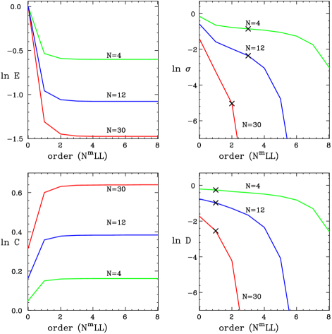
Figure 6: Evaluation of the Sudakov exponents with increasing logarithmic accuracy. The minimal term in the expansion is denoted by a cross.

Similar plots of the Sudakov exponents $\ln\tilde{J}(N,q^{2})$, $\ln\tilde{E}(N,q^{2},m^{2})$ and $\ln\tilde{\sigma}(N,q^{2},m^{2})$, of Eqs. (4.2), (62) and (59), respectively, are shown in the other boxes for a center-of-mass energy of $\sqrt{q^{2}}=M_{Z}$ and $\alpha_{s}^{\hbox{$\overline{\hbox{\tiny MS}}\,$}}(M_{Z}^{2})=0.118$. Here the fixed-logarithmic accuracy expansion is in powers of $A(M_{Z}^{2})$. It is clear that the divergence of the coefficient function is rather mild: $\ln\tilde{J}$ does not reach the minimal terms up to m=8; $\ln\tilde{E}$ converges and the Sudakov exponent of the total cross section $\ln\tilde{\sigma}$ reaches the minimal term at NNLL or at N³LL depending on $N$. Here the divergence is induced by the fragmentation subprocess.

When the expansion is truncated, e.g. at NLL order, the renormalon ambiguity does not appear but power accuracy is usually not reached. If one accepts that the DGE result (44) represents well the contribution of subleading logs, going to power accuracy simply requires avoiding any arbitrary fixed-logarithmic accuracy truncation. Since the series does not converge, a sensible possibility is to define the perturbative sum by truncation at the minimal term, i.e. just before the series starts diverging. The minimal term scales as a power. This definition was recently used [20] in the context of DGE for the deep inelastic structure function $F_{2}$, where a purely perturbative result was shown to be consistent with the data. However, in the case of the heavy-quark fragmentation considered here power corrections are particularly large and the series starts diverging already at low orders. In this case truncation at the minimal term would be far from optimal as it leads to discontinuities in the perturbative result as a function of $N$ whose magnitude is comparable to the power correction itself, thus inducing ${\cal O}(1)$ discontinuities in the non-perturbative contribution. The divergence of the coefficient function $\tilde{C}(N,q^{2})$ is much softer, so here truncation at the minimal term would be numerically sensible.

A better regularization prescription is to evaluate the Borel integral in Eq. (44) directly, with a Principal Value (PV) prescription applied at each pole. Fortran routines exist for evaluating such integrals efficiently provided that the exact position of the singularity is known, as in our case. This will therefore be our default prescription. All the numerical results for DGE we present below are obtained in this way.

5.1.2 Comparison between DGE and NLL resummation

We now compare the numerical results for NLL and DGE resummation with PV regularization. Our default parameters will be $\sqrt{q^{2}}=91.2$ GeV, $m=4.75$ GeV, $N_{f}=5$ and $\Lambda=0.243$ GeV, corresponding to $\alpha_{s}^{\hbox{$\overline{\hbox{\tiny MS}}\,$}}(M_{Z}^{2})=0.118$ and $\alpha_{s}^{\hbox{$\overline{\hbox{\tiny MS}}\,$}}(m^{2})=0.218$. We will be using a two-loop running coupling given by eqs. (32) and (33), or, explicitly, by [41]

$$\alpha_{s}^{\hbox{$\overline{\hbox{\tiny MS}}\,$}}(\mu^{2})=\frac{\pi}{\beta_{0}}\left(-\frac{1}{\delta}\frac{1}{1+w(s)}\right)\;,$$ (69)

where

$$w(s)\equiv W_{-1}\left(-\exp(-s/\delta-1)\right)\;,\qquad s\equiv\ln\frac{\mu^{2}}{\Lambda^{2}}\;,\qquad\delta\equiv\frac{\beta_{1}}{\beta_{0}^{2}}\;.$$ (70)

Here $W$ stands for the Lambert $W$ function [42].

Figure 7: Left: the matched heavy-quark fragmentation function $\tilde{D}(N,m^{2})$ with DGE (solid) and NLL (dashes) resummation. Right: the same for the $e^{+}e^{-}$ coefficient function $\tilde{C}(N,q^{2})$.

Figure 7 shows a comparison between the NLL and DGE resummed results for the heavy-quark fragmentation function $\tilde{D}(N,m^{2})$, and for the $e^{+}e^{-}$ coefficient function $\tilde{C}(N,q^{2})$ (both are matched according to (66) and (68) to the full ${\cal O}(\alpha_{s}$) result). One can immediately see that the NLL result for $\tilde{D}(N,m^{2})$ breaks down at $N=N_{L}=\exp(\pi/(2\beta_{0}\alpha_{s}(m^{2}))\sim 40$ where the $g^{(i)}_{\rm ini}$ functions become singular. The DGE result with PV regularization, on the other hand, remains moderate and shows no singular behavior. Indeed, owing to the procedure adopted where the Borel integrals are directly evaluated rather than expanded the DGE result is free of Landau singularities.

This does not mean, of course, that the perturbative DGE result by itself is physically meaningful: power corrections are needed. The advantage is, however, that this result, being free of spurious singularities, provides a good basis for the parametrization of power corrections for any $N$. In the case of $\tilde{C}(N,q^{2})$ the difference between the NLL and DGE results is much smaller than for $\tilde{D}(N,m^{2})$. The Landau singularity in the Sudakov-resummed coefficient function is located much further, at $N=\exp(\pi/(\beta_{0}\alpha_{s}(q^{2}))\sim 10^{6}$. Thus here subleading logs are smaller and power corrections can definitely be neglected.

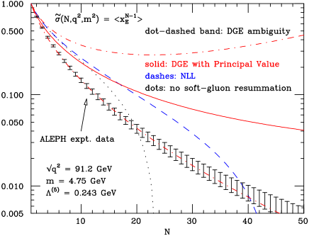
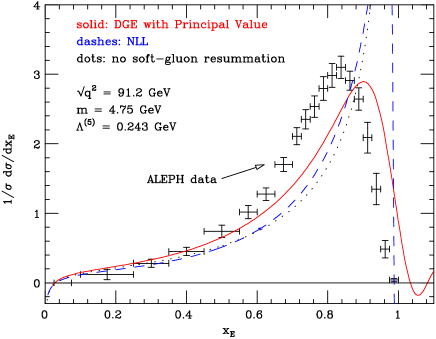
Figure 8: Left: a comparison between DGE and NLL for heavy-quark production in the $e^{+}e^{-}$ process. Right: the same curves in $x_{E}$ space. ALEPH [43] data are also shown.

Figure 8 shows a similar comparison for the full $e^{+}e^{-}$ cross section $\tilde{\sigma}(N,q^{2},m^{2})$ of Eq. (64). For reference we show also a curve with no soft gluon resummation as well as the experimental data from ALEPH [43]. The theoretical curves in $x_{E}$ space are obtained via numerical Mellin inversion:

$$D(x)=\frac{1}{2\pi i}\int_{\cal C}dN\;x^{-N}\tilde{D}(N)\;.$$ (71)

Figure 9: A prototype of the contour ${\cal C}$ employed in the numerical Mellin inversion to $x$ space.

In the NLL case the Minimal Prescription [44] is used: the contour ${\cal C}$ (see Fig. 9) passes between the origin and the leftmost Landau pole. In the case of the (PV-regularized) DGE result a specific prescription is not required since there are no Landau singularities. Any contour passing to the right of the origin would yield the same result. This may be surprising at first sight, since the original expression for the fragmentation function in $x$ space (30) does have a convergence constraint (see for example (36)). However, as we saw, when going to moment space this constraint is traded for renormalon singularities. Landau singularities instead appear only if the resummed expression is expanded in terms of the coupling. The inherent ambiguity of the perturbative description of the fragmentation function as $x\longrightarrow 1$ appears in the Borel sum as a renormalon ambiguity: In order to compensate for it one needs to specify an infinite set of power terms $(N\Lambda/m)^{n}$.

A hint about the size of such contributions can be obtained by considering different prescriptions for performing the Borel integration, PV being one of the possible choices. Evaluating $\ln\tilde{D}(N,m^{2})$ in (44) by going above and below the first pole at $u=1/2$ we obtain the band bounded by the dot-dashed curves in Fig. 8. The experimental data turn out to be within the band: This supports our expectation that one can describe them by modifying the resummed perturbative result with the first few power corrections.

5.2 Non-perturbative contributions

In general, the non-perturbative contribution to the fragmentation function should be included on top of the perturbative one through a convolution in $x$. Moments of the $B$-meson cross section as measured at LEP can then be written as the product of the perturbatively calculated moments $\tilde{\sigma}^{\hbox{\tiny PT}}(N,q^{2},m^{2})$ and the moments of some non-perturbative function.

Our first result is that at large $N$ and $m$ this function depends on the ratio $N\Lambda/m$ alone, up to corrections of order $1/N$. Unfortunately, with just one heavy flavour (charm is probably too light) the predictive power of this statement is largely lost: fixing $m$ the fragmentation can anyway depend only on $N$. This situation can be contrasted, for example, with the case of event-shape distributions where non-perturbative corrections can a priori depend on the centre-of-mass energy as well as on the shape variable: Thus the statement that the corrections can be described by a shape function of a single argument is already quite constraining [21, 19].

The emphasis in the phenomenological analysis is therefore on the particular dependence of the fragmentation function on $N\Lambda/m$ which is predicted by the renormalon model (48). Let us write

$$\tilde{\sigma}(N,q^{2},M^{2})\simeq\tilde{\sigma}^{\hbox{\tiny PT}}(N,q^{2},m^{2})\,\tilde{D}^{\hbox{\tiny NP}}_{\{\epsilon_{n}\}}((N-1)\Lambda/m)$$ (72)

where

$$\tilde{D}^{\hbox{\tiny NP}}_{\{\epsilon_{n}\}}((N-1)\Lambda/m)=\exp\left\{-\sum_{n=1}^{\infty}\epsilon_{n}\left(\frac{(N-1)\Lambda}{m}\right)^{n}\right\}.$$ (73)

The separation being, of course, ambiguous, the perturbative part in Eq. (72) describes the production of a bottom quark surrounded by a cloud of soft gluons and the non-perturbative one describes its hadronization into an observable $B$ meson. As before, we have not explicitly shown the dependence on the QCD scale $\Lambda$ which the perturbative part $\tilde{\sigma}^{\hbox{\tiny PT}}$ acquires via the strong coupling. The dependence of $\tilde{\sigma}(N,q^{2},M^{2})$ on the heavy meson mass $M$ rather than the heavy quark mass $m$ serves as a reminder that it refers to the observed particle.

In Eq. (73) we have made a few modifications compared to Eq. (48). Firstly, the factor $C_{F}/\beta_{0}$ has been included into the parameters $\epsilon_{n}$. Secondly, we have introduced a term proportional to $(N\Lambda/m)^{2}$, which is absent in the renormalon result. By including it and fitting to data we can examine this feature of the renormalon model (48). Finally, we have replaced $N\to N-1$. This modification is of course allowed in the large-$N$ limit, and it implements the constraint that for $N=1$ (i.e. the normalized total cross section) the non-perturbative correction vanishes. Eq. (72) will be the master equation for our phenomenological analyses of the LEP data. The default choice for the perturbative calculation of the $b$-quark differential cross section $\tilde{\sigma}^{\hbox{\tiny PT}}(N,q^{2},m^{2})$ will be the PV-regularized DGE.

5.2.1 The experimental data

Several experimental collaborations have recently published high-statistics and high-accuracy data for $B$-meson production in $e^{+}e^{-}$ collisions at the $Z^{0}$ peak, i.e. centre-of-mass energy around 91 GeV. Most of the data have been published in the form of differential distributions in the variable $x_{E}$, representing the ratio between the $B$-meson energy in the laboratory frame and the beam energy. The formal definition of the fragmentation function (1) is in terms of the longitudinal momentum fraction $x$. However, for large $q^{2}$ the two coincide: $x_{E}\simeq x$ up to corrections (3.2.1) of order $m^{2}/q^{2}$ which we neglect. From here on the two notations will be used interchangeably.

Data in $x$ space, along with their covariance matrices, have been published by the SLD [45], ALEPH [43], DELPHI [46] and OPAL [47] Collaborations. The DELPHI Collaboration has also published moment data, including the very important correlations between the moments up to $N=6$.

Rather than converting our moment-space expressions to $x$ space as usually done, we shall perform our fits directly in moment space, using the CERN Library minimization routine MINUIT [48]. Given the $x$-space data and covariance matrices as inputs, moments and their own covariance matrices can be calculated. The integral (4) defining Mellin moments can be replaced by a discrete sum over all the bins in $x$ space ($n_{\hbox{\tiny bins}}$ in total),

$$\tilde{\sigma}(N,q^{2},M^{2})\simeq\sum_{i=1}^{n_{\hbox{\tiny bins}}}x_{i}^{N-1}\Delta x_{i}f_{i},$$ (74)

where $f_{i}$ is the normalized value of the $i$-th bin, $x_{i}$ its central abscissa and $\Delta x_{i}$ its width. This equation represents a linear transformation of the vector $f_{i}$,

$$\underline{\tilde{\sigma}}={\bf A}\;\underline{f}\;,$$ (75)

and the matrix $\bf A$ is defined by $A_{Ni}\equiv x_{i}^{N-1}\Delta x_{i}$. Given the covariance matrix $\bf F$ for the $f_{i}$ values, one can build the covariance matrix $\bf S$ for the $\tilde{\sigma}(N,q^{2},M^{2})$ moments as

$${\bf S}={\bf A}\;{\bf F}\;{\bf A}^{T}\;.$$ (76)

$N$	ALEPH	DELPHI [46, 49]	DELPHI
2	0.7163 $\pm$ 0.0085	0.71422 $\pm$ 0.0052	0.7147 $\pm$ 0.0045
3	0.5433 $\pm$ 0.0097	0.5401 $\pm$ 0.0064	0.5413 $\pm$ 0.0057
4	0.4269 $\pm$ 0.0098	0.4236 $\pm$ 0.0065	0.4248 $\pm$ 0.0060
5	0.3437 $\pm$ 0.0096	0.3406 $\pm$ 0.0064	0.3419 $\pm$ 0.0059
6	0.2819 $\pm$ 0.0094	0.2789 $\pm$ 0.0061	0.2804 $\pm$ 0.0057
7	0.2345 $\pm$ 0.0091	-	0.2333 $\pm$ 0.0054
8	0.1975 $\pm$ 0.0087	-	0.1965 $\pm$ 0.0050
9	0.1680 $\pm$ 0.0084	-	0.1672 $\pm$ 0.0047
10	0.1441 $\pm$ 0.0080	-	0.1435 $\pm$ 0.0044
11	0.1245 $\pm$ 0.0076	-	0.1241 $\pm$ 0.0041
12	0.1084 $\pm$ 0.0072	-	0.1081 $\pm$ 0.0038
13	0.0949 $\pm$ 0.0069	-	0.0947 $\pm$ 0.0036
14	0.0835 $\pm$ 0.0065	-	0.0835 $\pm$ 0.0033
15	0.0738 $\pm$ 0.0062	-	0.0740 $\pm$ 0.0031
16	0.0656 $\pm$ 0.0058	-	0.0659 $\pm$ 0.0029
17	0.0585 $\pm$ 0.0055	-	0.0589 $\pm$ 0.0027
18	0.0524 $\pm$ 0.0052	-	0.0529 $\pm$ 0.0026
19	0.0471 $\pm$ 0.0049	-	0.0477 $\pm$ 0.0024
20	0.0425 $\pm$ 0.0047	-	0.0432 $\pm$ 0.0023
21	0.0384 $\pm$ 0.0044	-	0.0393 $\pm$ 0.0022

Table 1: Experimental data for normalized moments of weakly-decaying $B$-meson production in $e^{+}e^{-}$ collisions from the ALEPH and DELPHI Collaborations at LEP, evaluated according to Eq. (74) (left and right columns). The set in the central column corresponds to the five moments published by DELPHI in [46] (the $N=2$ point does not include here the correction for initial state electromagnetic radiation [49]).

Table 1 contains most of the moment-space data which will be used in the fits. Moments constructed from ALEPH and DELPHI data are shown. Moments higher than those shown in Table 1 can of course be calculated, and they have also been used in some of the fits. The amount of independent information they carry is however limited.

The central values reported in Table 1 show a very good agreement between the ALEPH and DELPHI sets. DELPHI moments are reported twice in the Table. The data in the central column are directly provided by [46, 49], where they were published in preliminary form, whereas we have calculated the ones in the right one according to Eq. (74). It should be noted that the DELPHI Collaboration extracted the moments directly from the unfolding program they used, rather than calculating them by summing up the published bins in $x$ space. This accounts for the small differences. The two sets of moments are, however, compatible within errors. For full consistency, we shall make use of the published set of moments with the published covariance matrix, and of our own values together with a covariance matrix we extract ourselves according to Eq. (76). The latter also presents some differences with the published one.

As a test of the fitting program, we have reproduced the fit that the DELPHI Collaboration performed in [46] to the five correlated moments which were published there, employing a so-called Kartvelishvili [6] functional form, $D^{\hbox{\tiny NP}}(\alpha,x)=(\alpha+1)(\alpha+2)x^{\alpha}(1-x)$. Using their parameters, their moments and covariance matrix, and NLL resummation only, we do recover their result: $\alpha=17.07\pm 0.57$, $\chi^{2}=114.7$ for $5-1$ degrees of freedom. However, fitting the moments we calculate ourselves (right column in Table 1) and using our own covariance matrix, we get instead $\alpha=14.30\pm 0.37$ and $\chi^{2}=159.8$. The apparent incompatibility of these results should mainly be attributed to the intrinsic failure of the fit, as indicated by the very large $\chi^{2}$ values. It also shows, however, how strong is the effect of small variations in the moments and in their covariances, due to the high degree of correlation and to the very small experimental errors. We have also performed the same fit to the first five ALEPH moments, obtaining $\alpha=21.5\pm 2.0$ and $\chi^{2}=15.1$.

We wish to point out that the very strong correlations between the experimental data for the moments are an important feature, which cannot be neglected when fitting a hadronization model. Extracting a meaningful covariance matrix for many moments at once is however no straightforward task. Because of the strong correlation between successive moments, inversion of such a matrix – needed when evaluating the $\chi^{2}$ for the fits – quickly becomes an intractable problem. In practice the numerical accuracy issue becomes acute when more than five or six consecutive moments are fitted together. Possible solutions are to use only a few moments or to pick non-consecutive moments. By means of these choices the matrix becomes smaller and the degree of correlation is lessened. One observes that matrices containing five or six moments, taken two or three moments apart, can be inverted with acceptable precision up to $N\sim 20$ . Using only three or four moments a sufficient numerical accuracy can be obtained up to $N\sim 30$. We make use of this expedient in some of the fits described below.

5.2.2 Fits to low moments

In order to test the renormalon model for the non-perturbative fragmentation function we would like to fit at least three parameters: $\Lambda$, $\epsilon_{1}$ and $\epsilon_{2}$. $\epsilon_{1}$ is the leading power correction corresponding to the shift of the entire distribution in $x$ space in units of $\Lambda/m$. It is expected to be of order $1$. Based on the renormalon model (48), $\epsilon_{2}$ is expected to vanish. Note that varying $\Lambda$, i.e. the value of $\alpha_{s}^{\hbox{$\overline{\hbox{\tiny MS}}\,$}}(M_{Z}^{2})$, influences both the perturbative and the non-perturbative parts of the cross section (72). Our approach to heavy-quark fragmentation can thus be tested by checking that the fit returns a value which is consistent with other determinations of $\alpha_{s}^{\hbox{$\overline{\hbox{\tiny MS}}\,$}}(M_{Z}^{2})$.

With this task in mind and the data described above at hand we should choose a subset of moments to be fitted. Theoretical limitations exist both for very small $N$ and for very large $N$. In the former case neither the soft-gluon perturbative resummation nor the power corrections of (48) are expected to dominate. In the latter, parametrizing just a few power corrections in the exponent may not be sufficient, as $N\Lambda/m$ is not small.

In this section we concentrate on moments up to $N=6$. In the next section we extend the analysis to higher moments. We use the correlated moments obtained from the ALEPH data and shown in Table 1. DELPHI moments have also been used for cross checks and comparisons but, due to their preliminary nature, we refrain from quoting these results.

	$\epsilon_{n}=0\,\,{\rm for}\,\,n\geq 3$
$\epsilon_{1}$	1.23 $\pm$ 0.23	1.03 $\pm$ 0.13	2.9 $\pm$ 1.5
$\epsilon_{2}$	0 (fixed)	0.011 $\pm$ 0.095	-1.1 $\pm$ 1.2
$\Lambda$ (GeV)	0.217 $\pm$ 0.025	0.243 (fixed)	0.138 $\pm$ 0.045
$\chi^{2}$/d.o.f	6.8/3	7.9/3	3.7/2

Table 2: Results of fits to ALEPH moments from $N=2$ to $N=6$.

First, we wish to extract $\Lambda$ and test the prediction that the leading power correction is of the order of $\Lambda/m$. We do this by fitting $\Lambda$ and $\epsilon_{1}$, setting $\epsilon_{n}=0$ for any $n\geq 2$ in Eq. (73). The results of this fit are shown in the first column of Table 2. The $\chi^{2}$ of the fit is reasonable albeit somewhat large. It is important to notice that the central value for $\Lambda$, corresponding to $\alpha_{s}^{\hbox{$\overline{\hbox{\tiny MS}}\,$}}(M_{Z}^{2})\simeq 0.117$, is fully compatible with present determinations of the strong coupling. The best fit value for $\epsilon_{1}$ is of order $1$, as expected. The resulting curves and the ALEPH data are shown in Fig. 10, both in $N$ and $x_{E}$ space.

Figure 10: Left: results of a fit for $\Lambda$ and $\epsilon_{1}$ (setting $\epsilon_{n}=0$ for $n\geq 2$) to ALEPH moments $N=2$ to $6$. Right: the corresponding curve in $x_{E}$ space, compared to the ALEPH and DELPHI data.

The overall description of the data is reasonable. This is quite remarkable given that, in $x_{E}$ space, the theoretical curve is no more than a shift of the PV-regularized DGE perturbative result.

The self-consistency of this fit can be probed by fitting now $\epsilon_{2}$ while fixing $\Lambda=0.243$ GeV. Being this value for $\Lambda$ compatible with the one returned by the previous fit, we expect to get a compatible value for $\epsilon_{1}$. The results are shown in the second column of Table 2. $\epsilon_{1}$ is indeed consistent with the one shown in the first column, the $\chi^{2}$ is similar, and $\epsilon_{2}$ turns out to be consistent with zero.

Finally, we attempt fitting three parameters, $\epsilon_{1}$, $\epsilon_{2}$ and $\Lambda$, simultaneously. The results are shown in the third column of Table 2. Consistency with previous fits appears rough, and the errors are extremely large.

Because of the problems encountered in the three-parameter fit, and since we expect the perturbative corrections we resum and the power correction we parametrize to become dominant at larger $N$, we now proceed to analyze higher moments.

5.2.3 Fits to high moments

In this section we wish to explore the possibility of fitting Eq. (72) to large-$N$ correlated moments. The large-$N$ region is challenging in several respects. Considering the data, the finite binning in $x_{E}$-space limits the amount of independent information contained in large-$N$ moments. On the theoretical side, as soon as the condition $N\Lambda/m\ll 1$ is violated the non-perturbative contribution is expected to become comparable to, and eventually to dominate, the perturbative one. Moreover, the exponentiation of power corrections can no longer be ignored and the specific form of (48), e.g. the vanishing of the second power of $N\Lambda/m$, becomes relevant. This makes this exercise particularly interesting: The validity of our model can really be tested. Yet, it is a priori not known up to what value of $N$ Eq. (48) with just a few parameters might hold: One should keep in mind that when going to extremely large $N$ the number of relevant parameters, corresponding to increasing powers of $N\Lambda/m$ in the exponent, increases, and the fitting procedure may get out of control.

$N$	$6,8,10,12,14,16$	$13,15,17,19$	$7,10,13,16,19$	$21,24,27,30$
$\epsilon_{1}$	0.831 $\pm$ 0.041	0.77 $\pm$ 0.15	0.96 $\pm$ 0.12	0.817 $\pm$ 0.056
$\epsilon_{2}$	-0.037 $\pm$ 0.007	-0.024 $\pm$0.028	-0.063 $\pm$ 0.025	-0.040 $\pm$ 0.008
$\Lambda$	0.261 $\pm$ 0.015	0.255 $\pm$0.025	0.238 $\pm$ 0.022	0.256 $\pm$ 0.020
$\chi^{2}$/d.o.f	11/3	8.3/1	9.0/2	3.3/1

Table 3: Fits to correlated ALEPH moments in the large-$N$ region. Only a few non-consecutive moments are used, as indicated in the various columns.

The moments we fit here are those we reconstructed from the $x_{E}$-space data and covariance matrices published by ALEPH. The fine binning in $x_{E}$ space of the ALEPH data helps in providing a good description of the large-$N$ moments in which we are interested. Provided that the correlations are properly taken into account, it allows one to consider moments as high as $N\simeq 30$.

In order to achieve a sufficiently accurate inversion of the covariance matrix we now make use of the expedient of using non-consecutive moments. The results, shown in Table 3, are remarkably consistent: Over a wide range of moments the best-fit values for $\Lambda$, $\epsilon_{1}$ and $\epsilon_{2}$ appear very similar, and in line with our expectations.

Figure 11: Results of fits to $\epsilon_{1}$, $\epsilon_{2}$ and $\Lambda$ (in GeV on the vertical axis) performed with correlated ALEPH moments within a “rolling window”, centered at $\bar{N}$, where 4 moments out of 7 are used. In the left plot the DGE perturbative result (with PV regularization) is used. In the right one instead the resummation is truncated at NLL accuracy.

We further explore the large-$N$ region by employing ‘rolling window’ fits, using again non-consecutive moments. Figure 11 shows fits to $\Lambda$, $\epsilon_{1}$ and $\epsilon_{2}$, performed within windows bordered by $\bar{N}\pm 3$, where only four correlated moments are used. At small $N$ the fits are inconclusive. As we saw above (Table 2) this is a consequence of trying to fit too many parameters. In the large-$N$ region the situation improves dramatically: $\epsilon_{2}$ tends to zero, as predicted by the renormalon model, and the value for $\Lambda$ stabilizes on $\sim$ 0.25 $\pm$ 0.04 GeV, corresponding to $\alpha_{s}^{\hbox{$\overline{\hbox{\tiny MS}}\,$}}(M_{Z}^{2})\simeq 0.118\pm 0.003$, which is compatible with other determinations. We stress that this should not be regarded as a reliable determination of the strong coupling as the analysis of experimental and theoretical errors was not performed. Note the fluctuations in the error bars at large $\bar{N}$ values, due to the deteriorating numerical accuracy.

For comparison, Fig. 11 also shows the same kind of fits with NLL resummation. The range in $N$ is limited here by the non-physical behavior of the resummed result for $N$ greater than 30 or so, as shown in Fig. 8. The results are clearly at variance with the DGE fits: $\Lambda$ and $\epsilon_{1}$ do not stabilize and $\epsilon_{2}$ does not tend to zero when $N$ becomes large.

5.2.4 Comparison with moment-space and $x_{E}$-space data

At the end of the day, one wishes of course to extract a parametrization for non-perturbative effects such that, when convoluted with the appropriate perturbative contribution, it allows for a fair description of the experimental data in both moment and $x_{E}$ space.

Figure 12: Left: results of a fit for $\Lambda$, $\epsilon_{1}$ and $\epsilon_{2}$ and to ALEPH moments $N=30,31,32$, setting $\epsilon_{n}=0$ for $n\geq 3$. Right: the corresponding curve in $x_{E}$ space, compared to the ALEPH and DELPHI data.

The experimental papers [45, 43, 46, 47] have tested a number of different parametrizations, and established which ones seem to offer a good description of the data. Our present attempt differs from theirs in several respects:

• we only fit data in moment space, and subsequently derive the corresponding $x_{E}$ distribution;

• our perturbative description is based on DGE, matched to the NLO result (66), and to the NLL Altarelli-Parisi evolution (64). The experiments instead usually use the perturbative fragmentation provided by Monte-Carlo programs. We recall that a non-perturbative function should only be used in connection with the same perturbative description it has been fitted with. Conversely, changing the perturbative description (or its parameters) can lead to fit vastly different non-perturbative functions;

• we use a renormalon-motivated functional form, Eq. (73), for the non-perturbative function, rather than phenomenological models like the commonly used Peterson et al. [7] or Kartvelishvili et al. [6]. Besides the theoretical reasons for using Eq. (73), we have also checked that the Kartvelishvili or Peterson functional forms do not provide a good description of the data when used with our DGE-improved perturbative result.

For illustrative purposes we perform a further fit using exclusively very high moments, $N=30,31$ and $32$. The main disadvantage of such a fit is that higher power corrections on the exponent, which are not parametrized but simply set to zero, may in fact play some role. On the other hand it has several advantages:

• one can be confident that the perturbative corrections resummed by (44) and the power correction parametrized by (48) indeed dominate.

• the stability observed in our previous fits at large $N$ guarantees that the result will be independent of the particular set of moment chosen.

• it ensures a good description of the large-$N$ limit, and thus of the region near $x\longrightarrow 1$.

The results are shown in Fig. 12. The fitted parameters (see the figure) are compatible with the ones shown in Table 3 and in Fig. 11. $\epsilon_{2}$, although not vanishing within the errors, is very small. In order to check the sensitivity to higher power corrections in the exponent, we have performed a similar fit (using $N=30,31$ and $32$) fixing $\epsilon_{2}\equiv 0$ and having $\Lambda$, $\epsilon_{1}$ and $\epsilon_{3}$ as free parameters. The result is visually similar to Fig. 12, but the parameters are somewhat different: $\Lambda=0.266\pm 0.020$, corresponding to $\alpha_{s}^{\hbox{$\overline{\hbox{\tiny MS}}\,$}}(M_{Z}^{2})\simeq 0.120$, and the parameters of the shape function are $\epsilon_{1}=0.86\pm 0.11$ and $\epsilon_{3}=-0.011\pm 0.003$. These differences with respect to Fig. 12 represent the sensitivity to higher power corrections.

Despite having used large-$N$ data only in the fit, the low-$N$ moments are fairly well described by the resulting curve, typically deviating by no more than a few percent. One can moreover notice that the whole curve in $x_{E}$ space is well reproduced, notwithstanding the fact that it was never directly fitted: Its shape is produced by the DGE-improved perturbative calculation, properly shifted and modeled by the fitted non-perturbative term (see also Fig. 8 for a comparison with the purely perturbative result). A better description of the lower moments and the region left of the peak is expected upon including corrections of order ${\cal O}((m^{2}/q^{2})\alpha_{s})$, non-logarithmic ${\cal O}(\alpha_{s}^{2})$ corrections [27], and power corrections of order $\Lambda/m$ not enhanced by $N$.

Note that the curve in $x_{E}$ space remains positive up to $x_{E}$ very close to one, and beyond the last experimental point. This constitutes a marked improvement with respect to fits based on fixed-order or NLL Sudakov-resummed perturbative results. In these approaches a convoluted non-perturbative function can be fitted to the data, and the resulting curve describes well the experimental points in the region below the peak. However, the cross section turns out negative over a broader region between the peak and $x_{E}=1$, and cannot therefore describe the last few data points. We recall that this improvement has been obtained here by refining the perturbative prediction, adding leading and subleading Sudakov logarithms within the DGE formalism and introducing an appropriate prescription (PV) to regularize the renormalons. This stands in contrast with the approach of [51] where large logarithmic corrections in the function $D(x,m^{2})$ are simply discarded.

6 Conclusions

In this paper we considered the problem of heavy-quark fragmentation in the large-$x$ region. We first derived a general relation (9) between the fragmentation function at large $N$ and a non-local hadronic matrix element at large light-cone separations. When combined with the result on the asymptotic form of this matrix element at large $m$ [14], it implies that the simultaneous limit where $N$ and $m$ get large together, with the ratio between them fixed, has a special status: the asymptotic heavy-quark fragmentation function depends on this ratio alone.

Equipped with this exact asymptotic result we proceeded to evaluate the fragmentation function perturbatively, resumming large logarithms of $N$ as well as running-coupling effect. We first calculated the splitting function of an off-shell gluon of a massive quark, from which we derived an all-order result for the fragmentation function in the large-$\beta_{0}$ limit. This result has some interesting features: in $x$ space it does not contain any renormalons, but it does have convergence constraints for $x\to 1$. In moment space these constraints are replaced by an infinite set of infrared renormalons, indicating certain non-perturbative corrections to the fragmentation function. The physical interpretation of this result is clear: the perturbative calculation only gives the probability of producing an on-shell quark with an energy fraction $x$ surrounded by a cloud of soft gluons, whereas the physical quantity (defined in the full theory) is the probability to produce a bound state (a heavy meson) with that energy fraction. The gap between the two is filled by these power corrections.

As expected, at large $N$ renormalon ambiguities depend only on the ratio $N\Lambda/m$. Thus, the non-perturbative contribution to the fragmentation function at large $x$ can be incorporated through a convolution with shape function of $m(1-x)$. Further details on this function can be deduced from the structure of the perturbative result:

• similarly to the logarithmically enhanced contributions, these power corrections exponentiate in moments space;

• the leading power correction is ${\cal O}(N\Lambda/m)$. Upon exponentiation it generates a shift of the perturbative spectrum in $x$ by an amount proportional to $\Lambda/m$;

• the second corrections in the exponent, ${\cal O}(N^{2}\Lambda^{2}/m^{2})$, is absent, suggesting that the shift may be a good approximation in a relatively wide range in $x$;

• higher order corrections such as ${\cal O}(N^{3}\Lambda^{3}/m^{3})$ which also appear in the exponent modify the shape of the spectrum near $x\sim 1$.

Regarding the non-perturbative fragmentation function as a set of non-perturbative power corrections is useful only if the perturbative sum itself is performed taking Sudakov logs as well as infrared renormalons into account. This is the purpose of DGE. The significance of Sudakov logs at large $x$ has long been understood, while that of renormalons is more subtle. In applications of Sudakov resummation in the asymptotic regime (e.g. in the coefficient function for a single-particle inclusive cross section at large $q^{2}$ – see Sec. 4 and 5) power corrections are negligible, and a fixed-logarithmic accuracy, e.g. NLL, is sufficient. For the heavy-quark fragmentation function, on the other hand, power corrections are essential, and therefore so is the proper separation between the perturbative sum and the power corrections. A proper separation can be achieved only if renormalons, which manifest themselves as subleading Sudakov logs, are resummed. Furthermore, we found that dealing with the renormalon ambiguity by means of a PV prescription, one avoids Landau singularities and obtains a sensible asymptotic behavior at large $N$.

The numerical analysis demonstrates the significance of this property. In contrast with the fixed-order result or even the NLL resummation, the DGE perturbative result with PV regularization (see Fig. 8), does not become large nor negative, but remains instead positive up to $x=1$. This is a result of refining the perturbative calculation for heavy-quark fragmentation, by including the effects of leading as well as subleading soft logarithms via DGE, while introducing a systematic prescription (PV) to separate the perturbative and non-perturbative contributions. Upon convolution with the properly fitted non-perturbative contribution, this feature allows for a good description of the data up to $x\simeq 1$.

While concentrating on the large-$x$ region, many other features of the fragmentation process have been simplified. We neglected power corrections in $m^{2}/q^{2}$ as well as perturbative corrections of order $\alpha_{s}^{2}$ which are not logarithmically enhanced. We also neglected power corrections of the type $\Lambda/m$ (not enhanced by $N$), which certainly play an important role at small $N$. All these aspects definitely deserve further investigation in the future. In spite of these simplifications and of the fact the non-perturbative correction we employ has minimal flexibility, we obtained a fairly good description (Fig. 10 and 12) of the ALEPH data on $B$-meson production. In doing so we extracted a value for $\alpha_{s}$ which is compatible with other determinations (although a systematic error analysis has not been performed here). We also found that the non-perturbative parameters for the fragmentation function match the expectations: the shift of the perturbative spectrum in $x$ is indeed of order $\Lambda/m$ and $\epsilon_{2}$ in Eq. (73) turns out to be very small.

Acknowledgments

We would like to thank Eli Ben-Haim, Volodya Braun, Stefano Catani, Alberto Guffanti, Gregory Korchemsky, Chris Sachrajda, Gavin Salam, George Sterman and Bryan Webber for very useful discussions. EG thanks the DFG for financial support. MC thanks the CERN Theory Division for hospitality and support.

References

- [1] J. C. Collins and D. E. Soper, Nucl. Phys. B194 (1982) 445.
- [2] P. Nason, in “Heavy Flavors”, A. J. Buras and M. . Lindner eds., Singapore, Singapore: World Scientific (1992) (Advanced series on directions in high energy physics, 10).
- [3] M. Cacciari and P. Nason, Phys. Rev. Lett. 89 (2002) 122003 [hep-ph/0204025].
- [4] P. Nason, “Heavy flavour production,” Talk given at the International Workshop on Heavy Quarks and Leptons, Vietri sul Mare, Salerno, Italy, 27 May - 1 Jun 2002 [hep-ph/0207362].
- [5] M. Cacciari, “Perturbative and non-perturbative issues in heavy quark fragmentation,” Talk given at the 37th Rencontres de Moriond on QCD and Hadronic Interactions, Les Arcs, France, 16-23 Mar 2002 [hep-ph/0205326].
- [6] V.G. Kartvelishvili, A.K. Likehoded and V.A. Petrov, Phys. Lett. B78 (1978) 615.
- [7] C. Peterson, D. Schlatter, I. Schmitt and P.M. Zerwas, Phys. Rev. D27 (1983) 105.
- [8] B. Mele and P. Nason, Phys. Lett. B245 (1990) 635.
- [9] Y. L. Dokshitzer, V. A. Khoze and S. I. Troian, J. Phys. G17 (1991) 1602.
- [10] Y. L. Dokshitzer, V. A. Khoze and S. I. Troian, Phys. Rev. D53 (1996) 89 [hep-ph/9506425].
- [11] S. Keller and E. Laenen, Phys. Rev. D59 (1999) 114004 [hep-ph/9812415].
- [12] S. Catani, S. Dittmaier and Z. Trocsanyi, Phys. Lett. B500 (2001) 149 [hep-ph/0011222].
- [13] M. Cacciari and S. Catani, Nucl. Phys. B617 (2001) 253 [hep-ph/0107138].
- [14] R. L. Jaffe and L. Randall, Nucl. Phys. B412 (1994) 79 [hep-ph/9306201].
- [15] P. Nason and B. R. Webber, Phys. Lett. B395 (1997) 355 [hep-ph/9612353].
- [16] M. Beneke, Phys. Rept. 317 (1999) 1 [hep-ph/9807443]; M. Beneke and V. M. Braun, “Renormalons and power corrections,” to be published in the Boris Ioffe Festschrift ’At the Frontier of Particle Physics / Handbook of QCD’, edited by M. Shifman (World Scientific, Singapore, 2001). [hep-ph/0010208].
- [17] E. Gardi and G. Grunberg, JHEP 9911 (1999) 016 [hep-ph/9908458].
- [18] E. Gardi and J. Rathsman, Nucl. Phys. B609 (2001) 123 [hep-ph/0103217]; Nucl. Phys. B638 (2002) 243 [hep-ph/0201019].
- [19] E. Gardi, “Soft and collinear radiation and factorization in perturbation theory and beyond,” Talk at the 37th Rencontres de Moriond on QCD and Hadronic Interactions, Les Arcs, France, 16-23 Mar 2002, and at Continuous Advances in QCD 2002 / ARKADYFEST (honoring the 60th birthday of Prof. Arkady Vainshtein), Minneapolis, Minnesota, 17-23 May 2002 [hep-ph/0206287].
- [20] E. Gardi and R. G. Roberts, “The interplay between Sudakov resummation, renormalons and higher twist in deep inelastic scattering,” [hep-ph/0210429].
- [21] G. P. Korchemsky and G. Sterman, Nucl. Phys. B437 (1995) 415 [hep-ph/9411211]; “Universality of infrared renormalons in hadronic cross sections”, Talk at the 30th Rencontres de Moriond: QCD and High Energy Hadronic Interactions, Meribel les Allues, France, 19-25 March 1995, Published in Moriond 1995: Hadronic:0383-392, [hep-ph/9505391]; Nucl. Phys. B555 (1999) 335 [hep-ph/9902341].
- [22] Y. L. Dokshitzer and B. R. Webber, Phys. Lett. B404 (1997) 321 [hep-ph/9704298].
- [23] E. Gardi, G. P. Korchemsky, D. A. Ross and S. Tafat, Nucl. Phys. B636 (2002) 385 [hep-ph/0203161].
- [24] G. P. Korchemsky and S. Tafat, JHEP 0010 (2000) 010 [hep-ph/0007005].
- [25] M. Cacciari, M. Greco, S. Rolli and A. Tanzini, Phys. Rev. D 55 (1997) 2736 [arXiv:hep-ph/9608213].
- [26] M. Cacciari and M. Greco, Phys. Rev. D 55 (1997) 7134 [arXiv:hep-ph/9702389].
- [27] P. Nason and C. Oleari, Nucl. Phys. B 565 (2000) 245 [arXiv:hep-ph/9903541].
- [28] S. Frixione and P. Nason, JHEP 0203 (2002) 053 [arXiv:hep-ph/0201281].
- [29] E. Gardi, Nucl. Phys. B622 (2002) 365 [hep-ph/0108222].
- [30] G. Grunberg, Phys. Lett. B304 (1993) 183.
- [31] E. G. Floratos, D. A. Ross and C. T. Sachrajda, Nucl. Phys. B129 (1977) 66 [Erratum-ibid. B139 (1978) 545].
- [32] J. A. Gracey, Nucl. Phys. B480 (1996) 73 [hep-ph/9609301].
- [33] S. Catani, B. R. Webber and G. Marchesini, Nucl. Phys. B349 (1991) 635.
- [34] G. P. Korchemsky and A. V. Radyushkin, Phys. Lett. B279 (1992) 359 [hep-ph/9203222].
- [35] G. P. Korchemsky and G. Marchesini, Nucl. Phys. B406 (1993) 225 [hep-ph/9210281]; Phys. Lett. B313 (1993) 433.
- [36] M. Beneke and V. M. Braun, Nucl. Phys. B454 (1995) 253 [hep-ph/9506452].
- [37] Y. L. Dokshitzer and B. R. Webber, Phys. Lett. B404 (1997) 321 [hep-ph/9704298].
- [38] E. Gardi, JHEP 0004 (2000) 030 [hep-ph/0003179].
- [39] G. Sterman, Nucl. Phys. B281 (1987) 310.
- [40] G. P. Korchemsky, Mod. Phys. Lett. A4 (1989) 1257.
-
[41]
E. Gardi and M. Karliner,
Nucl. Phys. B529 (1998) 383
[hep-ph/9802218];
E. Gardi, G. Grunberg and M. Karliner, JHEP 9807 (1998) 007 [hep-ph/9806462]. -
[42]
R.M. Corless, G.H. Gonnet, D.E.G. Hare, D.J. Jeffrey and D.E. Knuth,
“On the Lambert W Function”,
Adv. Comput. Math. 5 (1996) 329
K.M. Briggs, http://more.btexact.com/people/briggsk2/, for the implementation in C. - [43] A. Heister et al. [ALEPH Collaboration], Phys. Lett. B 512 (2001) 30 [hep-ex/0106051].
-
[44]
S. Catani, M. L. Mangano, P. Nason and L. Trentadue,
Phys. Lett. B378 (1996) 329
[hep-ph/9602208];
S. Catani, M. L. Mangano, P. Nason and L. Trentadue, Nucl. Phys. B478 (1996) 273 [hep-ph/9604351]. - [45] K. Abe et al. [SLD Collaboration], Phys. Rev. D 65 (2002) 092006 [Erratum-ibid. D 66 (2002) 079905] [hep-ex/0202031].
- [46] G. Barker et al. [DELPHI Collaboration], ICHEP 2002 Note, DELPHI 2002-069 CONF 603.
- [47] G. Abbiendi et al. [OPAL Collaboration], [hep-ex/0210031].
- [48] F. James and M. Roos, Comput. Phys. Commun. 10 (1975) 343.
- [49] E. Ben Haim, private communication
- [50] T. Boccali, private communication
-
[51]
J. Binnewies, B. A. Kniehl and G. Kramer,
Phys. Rev. D58 (1998) 014014
[hep-ph/9712482];
J. Binnewies, B. A. Kniehl and G. Kramer, Phys. Rev. D58 (1998) 034016 [hep-ph/9802231].