Kinematical Limits on Higgs Boson Production via Gluon Fusion in Association with Jets

Abstract:

In this paper, we analyze the high-energy limits for Higgs boson $+$ two jet production. We consider two high-energy limits, corresponding to two different kinematic regions: (a) the Higgs boson is centrally located in rapidity between the two jets, and very far from either jet; (b) the Higgs boson is close to one jet in rapidity, and both of these are very far from the other jet. In both cases the amplitudes factorize into impact factors or coefficient functions connected by gluons exchanged in the $t$ channel. Accordingly, we compute the coefficient function for the production of a Higgs boson from two off-shell gluons, and the impact factors for the production of a Higgs boson in association with a gluon or a quark jet. We include the full top quark mass dependence and compare this with the result obtained in the large top-mass limit.

1 Introduction

In hadronic collisions, Higgs boson production in association with two jets occurs through gluon-gluon fusion and through weak-boson fusion (WBF). The WBF process, $q\,q\to q\,q\,H$, occurs through the exchange of a $W$ or a $Z$ boson in the $t$ channel, and is characterized by two forward quark jets [1, 2]. This process will be crucial in trying to measure the Higgs boson couplings [3] at the Large Hadron Collider at CERN. In this respect, Higgs $+$ two jet production via gluon-gluon fusion, which has a much larger production rate before cuts, can be considered a background: it has the same final-state topology, and thus may hide the features of the WBF process. Luckily, the gluon-gluon fusion background can be reduced (but not eliminated) by requiring that the two jets are well-separated in rapidity and have a large invariant mass, $\sqrt{s_{j_{1}j_{2}}}$ [4, 5].

The calculation of Higgs $+$ two jet production via gluon-gluon fusion is quite involved, even at leading order in $\alpha_{s}$, because in this process the Higgs boson is produced via a heavy quark loop. Triangle, box, and pentagon quark loops occur, with by far the dominant contribution coming from the top quark. However, if the Higgs mass is smaller than the threshold for the creation of a top-quark pair, $M_{\scriptscriptstyle{\rm H}}\lesssim 2M_{t}$, the coupling of the Higgs to the gluons via a top-quark loop can be replaced by an effective coupling [6, 7]. That simplifies calculations tremendously, because it effectively reduces the number of loops in a given diagram by one. We shall term calculations using the effective coupling as being done in the large $M_{t}$ limit.

In fully inclusive Higgs production, the condition $M_{\scriptscriptstyle{\rm H}}\lesssim M_{t}$ is sufficient to use the large $M_{t}$ limit, because the only physical scales present in the production rate are the Higgs and the top-quark masses. However, in Higgs production in association with one or more jets, other kinematic invariants occur, like a Higgs-jet invariant mass or a dijet invariant mass (if there are two or more jets), or other kinematic quantities of interest, like the transverse energies of the Higgs or of the jets. In this instance, the condition $M_{\scriptscriptstyle{\rm H}}\lesssim M_{t}$ may not be sufficient to use the large $M_{t}$ limit.

Recently, we computed the scattering amplitudes and the cross section for the production of a Higgs boson through gluon-gluon fusion, in association with two jets, including the full $M_{t}$ dependence [4, 5], and have used it as a benchmark to test the large $M_{t}$ limit. We found that in order to use the large $M_{t}$ limit, in addition to the necessary condition $M_{\scriptscriptstyle{\rm H}}\lesssim 2M_{t}$, the jet transverse energies must be smaller than the top-quark mass, $p_{{}\scriptscriptstyle\perp}\lesssim M_{t}$. That agrees with the analysis of the large $M_{t}$ limit in the context of Higgs $+$ one jet production [8]. However, we also found that the large $M_{t}$ approximation is quite insensitive to the value of the Higgs–jet and/or dijet invariant masses. This issue becomes important in the context of its companion process: the isolation of Higgs production via WBF requires selecting on events with large dijet invariant mass. This cut suppresses the gluon-gluon fusion contribution and reduces the QCD backgrounds.

In this paper, we consider in more detail the high-energy limit for Higgs $+$ two jet production via gluon-gluon fusion. To be precise, we term the high-energy limit to mean the cases when Higgs–jet and/or dijet invariant masses become much larger than the typical momentum transfers in the scattering. In addition to being crucial for the study of Higgs-boson couplings through the WBF process, this limit is also interesting per se. In fact, in the high-energy limit the scattering amplitude factorizes into high-energy coefficient functions, or impact factors, connected by a gluon exchanged in the $t$ channel. We can obtain the amplitudes for different sub-processes by assembling together different impact factors. Thus the high-energy factorization constitutes a stringent consistency check on any amplitude for the production of a Higgs plus one or more jets. In addition, the high-energy factorization is independent of the large $M_{t}$ limit, i.e. the two limits must commute.

In the high-energy limit, one deals with a kinematic region characterized by two (or more) very different hard scales. In the instances above, a large scale, of the order of the squared parton center-of-mass energy $s$, can be either a Higgs–jet or a dijet invariant mass. A comparatively smaller scale, of the order of a momentum transfer $t$, can be a jet (or Higgs) transverse energy. If it is found that a fixed-order expansion of the parton cross section in $\alpha_{\scriptscriptstyle S}$ does not suffice to describe the data for the production rate under examination, then it may be necessary to resum the large logarithms of type $\ln(s/|t|)$. This can be done through the BFKL equation [9, 10, 11], which is an equation for the (process independent) Green’s function of a gluon exchanged in the $t$ channel between (process dependent) impact factors.

As a warm-up, we analyze in Section 2 the high-energy factorization in a simpler case: Higgs $+$ one jet production in proton-(anti)proton, $pp$, scattering. We obtain the impact factor for producing a lone Higgs and compare the high-energy limit with and without the large $M_{t}$ approximation. In Section 3, we present the amplitudes for $q\,Q\to q\,Q\,H$ and $q\,g\to q\,g\,H$ scattering, already computed in Ref. [5], in a different form, which is more convenient to analyze the high-energy limits. In Section 4, we consider the high-energy factorization for Higgs $+$ two jet production, and analyze the two high-energy limits which can occur in this case: (a) the Higgs boson centrally located in rapidity between the two jets, and very far from either jet; (b) with the Higgs boson close to one jet in rapidity, and both of these very far from the other jet. In the first case we compute the coefficient function for the production of a Higgs from two off-shell gluons, and in the second case we compute the impact factors for the production of a Higgs in association with a gluon or a quark jet. Again we include the full top quark mass dependence and compare this with the result obtained in the large $M_{t}$ limit. Finally, in Section 5, we draw our conclusions.

2 High-energy factorization of Higgs + one jet

The process $pp\to jH$ occurs through gluon-gluon fusion, with the Higgs boson coupling to the gluons via a quark loop. Representative amplitudes for this process are given in Fig. 1. All momenta are taken outgoing and the relevant squared-energy scales are the parton center-of-mass energy $s=(p_{a}+p_{b})^{2}$, the momentum transfer $t=(p_{a}+p_{H})^{2}$, the Higgs mass $M_{\scriptscriptstyle{\rm H}}$, the top-quark mass $M_{t}$ and the jet-Higgs invariant mass $s_{j\scriptscriptstyle{\rm H}}$. At leading order, $s=s_{j\scriptscriptstyle{\rm H}}$ and $s+t+u=M_{\scriptscriptstyle{\rm H}}^{2}$, where $u=(p_{a}+p_{b^{\prime}})^{2}$.

The corresponding scattering amplitudes have been computed in Ref. [12].

The high-energy limit for this process is given by $s_{j\scriptscriptstyle{\rm H}}\gg|t|,M_{\scriptscriptstyle{\rm H}}^{2}$, where the jet-Higgs mass is of the order of the center-of-mass energy (equal at leading order), and is much larger than any other invariant. This implies that the rapidity interval between the jet and the Higgs is large. This limit has been investigated before in Ref. [13], where the BFKL resummation of the logarithms of type $\ln(s/|t|)$ was performed. We now review the results of this analysis in Section 2.1.

2.1 The high-energy limit for Higgs + one jet

We consider the production of a parton of momentum $p_{b^{\prime}}$ and a Higgs boson of momentum $p_{\scriptscriptstyle{\rm H}}$, in the scattering between two partons of momenta $p_{a}$ and $p_{b}$. The high-energy limit, $s_{j\scriptscriptstyle{\rm H}}\gg|t|,\,M_{\scriptscriptstyle{\rm H}}^{2}$, is equivalent to requiring a strong ordering of the light-cone components of the final-state momenta, i.e. the multi-Regge kinematics [9]

$$p_{\scriptscriptstyle{\rm H}}^{+}\gg p_{b^{\prime}}^{+}\,,\qquad p_{\scriptscriptstyle{\rm H}}^{-}\ll p_{b^{\prime}}^{-}\,,$$ (1)

where we have introduced light-cone coordinates $p^{\pm}=p_{0}\pm p_{z}$, and complex transverse coordinates $p_{\perp}=p_{x}+ip_{y}$ (see Appendix D). Equation (1) implies that the rapidities are ordered as

$$y_{\scriptscriptstyle{\rm H}}\gg y_{b^{\prime}}+\left|\ln{m_{\scriptscriptstyle{{\rm H}_{\perp}}}\over|p_{b^{\prime}\scriptscriptstyle\perp}|}\right|\,,$$ (2)

with $m_{\scriptscriptstyle{{\rm H}_{\perp}}}=\sqrt{M_{\scriptscriptstyle{\rm H}}^{2}+|p_{\scriptscriptstyle{{\rm H}_{\perp}}}|^{2}}$ the Higgs transverse mass.

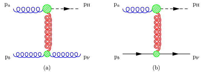
Figure 1: $(a)$ Amplitudes for $g\,g\to H\,g$ scattering, and $(b)$ for $g\,q\to H\,q$ scattering in the high-energy limit (2). The diagrams shown are meant to visualize the scattering amplitude only, and have no direct relation to Feynman diagrams.

In the high-energy limit, the production rate is dominated by the parton sub-processes which feature gluon exchange in the $t$ channel, represented by a double curly line in Fig. 1. The leading sub-processes are: $g\,g\to g\,H$, Fig. 1 (a) and $q\,g\to q\,H$, Fig. 1 (b). Since they only differ by the color strength in the jet-production vertex, it is enough to consider one of them and include the others through the effective parton distribution function (p.d.f.) [14]

$$f_{\rm eff}(x,\mu_{F}^{2})=G\left(x,\mu_{F}^{2}\right)+{C_{F}\over C_{A}}\sum_{f}\left[Q_{f}\left(x,\mu_{F}^{2}\right)+\bar{Q}_{f}\left(x,\mu_{F}^{2}\right)\right],$$ (3)

where the sum runs over the quark flavours. In the high-energy limit, the amplitude for $g\,g\to g\,H$ can be written in terms of an effective vertex for the production of a gluon jet, $g^{*}\,g\rightarrow g$ (the lower blob in Fig. 1 (a)), and an effective vertex for the production of a Higgs boson, $g^{*}\,g\rightarrow H$ (the upper blob in Fig. 1 (a)),

$$i\ {\cal M}^{gg\to Hg}\left(p_{a}^{\nu_{a}},p_{\scriptscriptstyle{\rm H}};p_{b^{\prime}}^{\nu_{b^{\prime}}},p_{b}^{\nu_{b}}\right)=2\,s\left[\delta^{ac}C^{g;\scriptscriptstyle H}\left(p_{a}^{\nu_{a}};p_{\scriptscriptstyle{\rm H}}\right)\right]{1\over t}\left[ig\,f^{bb^{\prime}c}\,C^{g;g}\left(p_{b}^{\nu_{b}};p_{b^{\prime}}^{\nu_{b^{\prime}}}\right)\right]\,,$$ (4)

with $q=p_{b}+p_{b^{\prime}}$, $t\simeq-|q_{\scriptscriptstyle\perp}|^{2}$, and the $\nu$’s labelling the gluon helicities . Using the high-energy factorization of the amplitude, the effective vertices for $g^{*}\,g\rightarrow g$ can be obtained from $g\,g\to g\,g$ scattering [15]. We define the impact factor as the square of each term in squared brackets in Eq. (4), summed (averaged) over final (initial) helicities and colors. Thus the impact factor for the gluon jet is [16]

$$I^{g;g}(p_{b};p_{b^{\prime}}) = \frac{1}{2(N_{c}^{2}-1)}\left[ig\,f^{bb^{\prime}c}\,C^{g;g}\left(p_{b}^{\nu_{b}};p_{b^{\prime}}^{\nu_{b^{\prime}}}\right)\right]\left[-ig\,f^{bb^{\prime}d}\,\left[C^{g;g}\left(p_{b}^{\nu_{b}};p_{b^{\prime}}^{\nu_{b^{\prime}}}\right)\right]^{*}\right]$$ (5)

$$= g^{2}\,{C_{A}\over N_{c}^{2}-1}\,\delta^{cd}\,,$$

with $C_{A}=N_{c}$ = 3, and implicit sums over repeated indices. The impact factor for Higgs production is

$$I^{g;\scriptscriptstyle H}(p_{a};p_{\scriptscriptstyle{\rm H}})=\frac{1}{2(N_{c}^{2}-1)}\left[\delta^{ac}C^{g;\scriptscriptstyle H}\left(p_{a}^{\nu_{a}};p_{\scriptscriptstyle{\rm H}}\right)\right]\left[\delta^{ad}\left[C^{g;\scriptscriptstyle H}\left(p_{a}^{\nu_{a}};p_{\scriptscriptstyle{\rm H}}\right)\right]^{*}\right]\,.$$ (6)

The squared amplitude, summed (averaged) over final (initial) helicities and colors, can be written as

$$\left|{\cal M}^{gg\to Hg}\right|^{2}={4s^{2}\over t^{2}}\,I^{g;\scriptscriptstyle H}(p_{a};p_{\scriptscriptstyle{\rm H}})\,I^{g;g}(p_{b};p_{b^{\prime}})\,.$$ (7)

Note that this squared amplitude also has a sum over the colors of the gluons in the $t$-channel, the indices of which are implicitly included in the impact factors. From the squared amplitude for $g\,g\to g\,H$ in the high-energy limit [13], we can extract the impact factor for Higgs production

$$I^{g;\scriptscriptstyle H}(p_{a};p_{\scriptscriptstyle{\rm H}})=\frac{1}{N_{c}^{2}-1}\,{\alpha_{\scriptscriptstyle S}^{2}\over v^{2}}\,{1\over 128\pi^{2}}\,\delta^{cd}\,|q_{\scriptscriptstyle\perp}|^{2}\,\left|{\cal F}\left(|q_{\scriptscriptstyle\perp}|^{2}\right)\right|^{2}\,,$$ (8)

where $v$ is the vacuum expectation value parameter, $v^{2}=(G_{F}\sqrt{2})^{-1}\simeq(246.22~{}{\rm GeV})^{2}$ and ${\cal F}(|q_{\scriptscriptstyle\perp}|^{2})$ is given by [13]

$${\cal F}\left(|q_{\scriptscriptstyle\perp}|^{2}\right) = \left({4M_{t}^{2}\over m_{\scriptscriptstyle{{\rm H}_{\perp}}}^{2}}\right)\left\{-2\,-\,\left({2|q_{\scriptscriptstyle\perp}|^{2}\over m_{\scriptscriptstyle{{\rm H}_{\perp}}}^{2}}\right)\left[\sqrt{b}\,W(b)-\sqrt{a}\,W(a)\right]\right.$$ (9)

$$+ \left.{1\over 2}\left(1-{4M_{t}^{2}\over m_{\scriptscriptstyle{{\rm H}_{\perp}}}^{2}}\right)\left[W(b)^{2}-W(a)^{2}\right]\right\}\,,$$

with

$$W(c)\ =\ \cases{\phantom{\bigg{[}}\!-2i\arcsin{(1/\sqrt{1-c})}\ ,&$\qquad\qquad c<0$\cr\phantom{\bigg{[}}\!\ln\displaystyle{1+\sqrt{c}\over 1-\sqrt{c}}\,-\,i\pi\ ,&$\qquad\qquad 0<c<1$\cr\phantom{\bigg{[}}\!\ln\displaystyle{\sqrt{c}+1\over\sqrt{c}-1}\ ,&$\qquad\qquad c>1$\cr}$$

and

$$a=1+{4M_{t}^{2}\over|q_{\scriptscriptstyle\perp}|^{2}}\,,\qquad b=1-{4M_{t}^{2}\over M_{\scriptscriptstyle{\rm H}}^{2}}\,,$$ (10)

and we take the root $\sqrt{b}=i\sqrt{|b|}$ for $b<0$.

The amplitude for $q(\bar{q})\,g\to q(\bar{q})\,H$ scattering, Fig. 1 (b), has the same analytic form as Eq. (4), up to the replacement of an incoming gluon with a quark. If that occurs on the lower line, we perform the substitution

$$ig\,f^{bb^{\prime}c}\,C^{g;g}\left(p_{b}^{\nu_{b}};p_{b^{\prime}}^{\nu_{b^{\prime}}}\right)\leftrightarrow g\,T^{c}_{b^{\prime}\bar{b}}\,C^{\bar{q};q}\left(p_{b}^{-\nu_{b^{\prime}}};p_{b^{\prime}}^{\nu_{b^{\prime}}}\right)\,,$$ (11)

and similar ones for an antiquark and/or for the upper line. The effective vertices for the production of a quark jet, $g^{*}\,q\rightarrow q$ are given in Ref. [17, 18]. Then the impact factor for the quark jet is [16] 

$$I^{\bar{q};q}(p_{b};p_{b^{\prime}}) = \frac{1}{2N_{c}}\left[g\ T^{c}_{b^{\prime}\bar{b}}\,C^{\bar{q};q}\left(p_{b}^{-\nu_{b^{\prime}}};p_{b^{\prime}}^{\nu_{b^{\prime}}}\right)\right]\left\{g\ T^{d}_{\bar{b}b^{\prime}}\,\left[C^{\bar{q};q}\left(p_{b}^{-\nu_{b^{\prime}}};p_{b^{\prime}}^{\nu_{b^{\prime}}}\right)\right]^{*}\right\}$$ (12)

$$= g^{2}\,{1\over 2N_{c}}\,\delta^{cd}\,.$$

The ratio of the impact factor for the quark above to the one of the gluon (5) is the color factor $C_{F}/C_{A}$ of the effective p.d.f. (3).

2.2 The combined high-energy limit and large top-mass limit

In the large top-mass limit, Eq. (9) reduces to [13]

$$\lim_{|q_{\scriptscriptstyle\perp}|,\,M_{\scriptscriptstyle{\rm H}}\,\ll\,M_{t}}{\cal F}\left(|q_{\scriptscriptstyle\perp}|^{2}\right)=-{4\over 3}$$ (13)

and the impact factor $g^{*}\,g\rightarrow H$ for Higgs production becomes

$$\lim_{|q_{\scriptscriptstyle\perp}|,\,M_{\scriptscriptstyle{\rm H}}\,\ll\,M_{t}}I^{g;\scriptscriptstyle H}(p_{a};p_{\scriptscriptstyle{\rm H}})=\frac{1}{N_{c}^{2}-1}{A^{2}\over 8}\delta^{cd}\,|q_{\scriptscriptstyle\perp}|^{2}\,,$$ (14)

where

$$A=\frac{\alpha_{\scriptscriptstyle S}}{3\pi v}\,.$$ (15)

Alternatively, the impact factor can be obtained directly in the large $M_{t}$ limit, which is simplified by using a Lagrangian with an effective Higgs-gluon-gluon operator, as discussed in Appendix F. In this approach the constant $A$ above is just the coupling of the effective operator (see Eq. (111)). The relevant sub-amplitudes in the large $M_{t}$ limit are given in Appendix F.2, and for Higgs plus three gluons, only the sub-amplitude (115) is leading in the high-energy limit. Using the decomposition (F.1), we can then write the amplitude for $g\,g\to H\,g$ in the form of Eq. (4) with effective vertex $g^{*}\,g\to H$

$$C^{\scriptscriptstyle H}(p_{a}^{-};p_{\scriptscriptstyle{\rm H}})=-i{A\over 2\sqrt{2}}\,q_{\scriptscriptstyle\perp}\,.$$ (16)

Using Eqs. (6) and (16), we obtain the same result (14) as above for the impact factor for Higgs production $g^{*}\,g\to H$ in the large top-mass limit. This verifies that the two limits commute. It is easy to check that the large $M_{t}$ amplitudes for $q\,g\rightarrow q\,H$ also factorize in the high-energy limit as expected.

2.3 The production rate for Higgs + one jet

Using the squared-matrix element formula (7), it is straightforward to compute the high-energy limit of the differential cross section for a Higgs boson with an associated jet in hadron-hadron collisions. For this one must keep in mind that the Higgs boson rapidity may be either much larger than the jet rapidity (as given by the limits (1) and (2)) or much smaller than the jet rapidity (obtained by reversing the limits in (1) and (2)).

 

Figure 2: Transverse momentum distribution of the Higgs boson (and of the jet) in $H$ + one jet production in $pp$ collisions at the LHC energy $\sqrt{s}=14$ TeV. The rapidity difference between the jet and the Higgs is taken to be $\Delta y=3$. The Higgs mass has been fixed to $M_{\scriptscriptstyle{\rm H}}=120$ GeV in the left panel, and to $M_{\scriptscriptstyle{\rm H}}=480$ GeV in the right panel. The curves show the leading order amplitudes computed exactly (solid line) with top mass $M_{t}=175$ GeV, in the $M_{t}\,\to\,\infty$ limit (dotted line) and in the high-energy limit (dashed line).

In Fig. 2, we plot the transverse momentum distribution of the Higgs boson (and of the jet) in $H$ + one jet production in $pp$ collisions at the LHC energy $\sqrt{s}=14$ TeV. The rapidity difference between the jet and the Higgs is taken to be $\Delta y=3$. The top-quark mass has been fixed to $M_{t}=175$ GeV while the the Higgs mass has been chosen to be $M_{\scriptscriptstyle{\rm H}}=120$ GeV in the left panel, and $M_{\scriptscriptstyle{\rm H}}=480$ GeV in the right panel. The curves in Fig. 2 (all at leading order in $\alpha_{s}$) correspond to the exact evaluation of the production rate, according to the formulae of Ref. [12] (solid line); to the rate with the amplitudes evaluated in the $M_{t}\,\to\,\infty$ limit, as given in Section F.2 (dotted line); and to the rate evaluated in the high-energy limit, according to the results of Section 2.1 (dashed line). We use the exact production rate as a benchmark to which to compare the large $M_{t}$ limit and the high-energy limit.

For the lower range of transverse momenta and for $M_{\scriptscriptstyle{\rm H}}\lesssim 2M_{t}$ (left panel), the large $M_{t}$ limit approximates the exact calculation very well, but begins to deviate from it for $p_{\perp}\gtrsim M_{\scriptscriptstyle{\rm H}}$ [8]. Note that the large $M_{t}$ limit fares well even though $M_{t}$ is not the largest kinematic invariant. In fact, for $M_{\scriptscriptstyle{\rm H}}=120$ GeV, and $p_{\perp}>50~{}$GeV, the jet-Higgs invariant mass is $\sqrt{s_{j\scriptscriptstyle{\rm H}}}\gtrsim 390$ GeV. This behavior is confirmed from the analysis of the transverse momentum distribution at larger values of $\Delta y$: the large $M_{t}$ limit is insensitive to the value of the jet-Higgs invariant mass. This is not unexpected, since at large values of $\Delta y$ the cross section is effectively dominated by diagrams with gluon exchange in the $t$ channel, as displayed in Fig. 1. Thus it is well described by the high-energy factorization of Section 2.1. When, in addition, we take the large $M_{t}$ limit, this does not modify the high-energy factorization, but only the impact factor for Higgs production, as in Section 2.2. In the high-energy limit, the sensitivity to the full $M_{t}$-dependence does not occur globally at the level of the entire amplitude, but locally (in rapidity) at the level of the impact factor for Higgs production.

For $M_{\scriptscriptstyle{\rm H}}\gtrsim 2M_{t}$ (right panel), the large $M_{t}$ limit does no longer approximate the exact solution, while the high-energy limit only gets slightly worse, due to the $M_{\scriptscriptstyle{\rm H}}$ dependence in Eq. (2), over the entire range of transverse momenta and for this rapidity separation.

3 Exact amplitudes for Higgs + two jets

We are interested in the high-energy limit of Higgs + two jet production in $pp$ scattering, $pp\rightarrow j_{1}j_{2}H$, via gluon-gluon fusion. We computed the exact leading order amplitudes, including the full dependence on the top quark mass $M_{t}$, in Ref. [5].

In this section we give analytic formulae for the amplitudes for $q\,Q\to q\,Q\,H$ and $q\,g\to q\,g\,H$ scattering in an alternate form that is more suitable for extracting the high-energy limit. We shall see that these amplitudes are sufficient to obtain the relevant production vertices and impact factors in the high-energy limit. Because of their complexity, we do not give the expressions for the $g\,g\to g\,g\,H$ here, although in principle, they could be used as an analytic cross-check. Instead we have performed this cross-check numerically.

3.1 The amplitude for $\boldsymbol{q\,Q\to q\,Q\,H}$ scattering

There is one Feynman diagram for $q\,Q\to q\,Q\,H$ scattering, obtained by inserting a $g\,g\,H$ triangle-loop coupling  on the gluon exchanged in the $t$ channel of the corresponding $q\,Q\to q\,Q$ diagram. The color decomposition of the amplitude is identical to the corresponding QCD amplitude

$${\cal M}\left(1_{q},2_{\bar{q}};3_{Q},4_{{\overline{Q}}}\right)=g^{2}\left(T^{a}\right)_{i_{1}}^{{\bar{\imath}}_{2}}\,\left(T^{a}\right)_{i_{3}}^{{\bar{\imath}}_{4}}\,m\left(1_{q},2_{\bar{q}};3_{Q},4_{{\overline{Q}}}\right)\,.$$ (17)

For simplicity we treat all momenta as outgoing (with $p_{H}+p_{1}+p_{2}+p_{3}+p_{4}=0$), and we write the helicity amplitudes in terms of products of massless Weyl spinors $\psi_{\pm}(p)$ of fixed helicity

$$\psi_{\pm}(p)={1\pm\gamma_{5}\over 2}\psi(p)\equiv|p^{\pm}\rangle\,,\qquad\overline{\psi_{\pm}(p)}\equiv\langle p^{\pm}|\,.$$ (18)

We use the following notation [19] for spinor products

$$\langle pk\rangle\equiv\langle p^{-}|k^{+}\rangle\,,\qquad\left[pk\right]\equiv\langle p^{+}|k^{-}\rangle\,,\qquad{\rm with}\;\;\langle pk\rangle^{*}={\rm sign}(p^{0}k^{0})\left[kp\right]\,,$$ (19)

currents

$$\langle i|k|j\rangle \equiv \langle i^{-}|/\!\!\!k|j^{-}\rangle=\langle ik\rangle\left[kj\right]\,,$$

$$\langle i|(k+l)|j\rangle \equiv \langle i^{-}|(/\!\!\!k+/\!\!\!l)|j^{-}\rangle=\langle i|k|j\rangle+\langle i|l|j\rangle\,,$$ (20)

and Mandelstam invariants

$$s_{pk}=2\,p\cdot k=\langle pk\rangle\left[kp\right]\,.$$ (21)

There is only one independent sub-amplitude, which we obtain by saturating the off-shell gluons from the triangle loop (72) with two fermion currents

$$i\,m\left(1_{q}^{+},2_{\bar{q}}^{-};3_{Q}^{+},4_{{\overline{Q}}}^{-}\right)$$ (22)

$$= 4\ {g^{2}M_{t}^{2}\over\ v}\ {{\langle 2|(3+4)|1\rangle}{\langle 4|(1+2)|3\rangle}A_{1}(12;34)-2\left[1\,3\right]\left\langle 4\,2\right\rangle A_{2}(12;34)\over s_{12}s_{34}}\,,$$

where the functions $A_{1,2}(12;34)\equiv A_{1,2}(p_{1}+p_{2};\,p_{3}+p_{4})$ are the two independent form factors from the triangle loop, defined in Eq. (81). They are related to the form factors $F_{T}$ and $F_{L}$ of Ref. [5] by

$$A_{1}(q_{1},q_{2})={i\over(4\pi)^{2}}F_{T}\;,\qquad A_{2}(q_{1},q_{2})={i\over(4\pi)^{2}}\left(F_{T}\ q_{1}\cdot q_{2}+F_{L}\ q_{1}^{2}q_{2}^{2}\right)\;.$$ (23)

All other helicity configurations are related to Eq. (22) by parity inversion and charge conjugation, except for the $(+--+)$ configuration, which can be obtained by inverting one of the two quark currents. The $Q{\overline{Q}}$ quark current, for example, is inverted by re-labeling 3 and 4. For identical quarks, we must subtract from Eq. (17) the same term with the quarks (but not the anti-quarks) exchanged ($1_{q}\leftrightarrow 3_{Q}$).

3.2 The amplitude for $\boldsymbol{q\,g\to q\,g\,H}$ scattering

The diagrams for $q\,g\to q\,g\,H$ scattering are obtained from the three corresponding $q\,g\to q\,g$ amplitudes by inserting a $g\,g\,H$ triangle-loop coupling on any gluon line or by replacing the three-gluon coupling with a $g\,g\,g\,H$ box loop. There are three distinct box diagrams corresponding to the three distinct orderings of the gluon momenta. This gives a total of 10 diagrams: 7 with triangles and 3 with boxes. The color decomposition of the amplitude is identical to the corresponding QCD amplitude

$${\cal M}\left(1,2;3_{q},4_{{\bar{q}}}\right)=g^{2}\left[\left(T^{a_{1}}T^{a_{2}}\right)_{i_{3}}^{{\bar{\imath}}_{4}}m\left(1,2;3_{q},4_{{\bar{q}}}\right)+\left(T^{a_{2}}T^{a_{1}}\right)_{i_{3}}^{{\bar{\imath}}_{4}}m\left(2,1;3_{q},4_{{\bar{q}}}\right)\right]\,.$$ (24)

There are only three independent helicity sub-amplitudes, which we take to be $m(1^{+},2^{-};3_{q}^{+},4_{{\bar{q}}}^{-})$, $m(1^{-},2^{+};3_{q}^{+},4_{{\bar{q}}}^{-})$ and $m(1^{+},2^{+};3_{q}^{+},4_{{\bar{q}}}^{-})$. All others can be obtained by parity inversion, reflection symmetry, and charge conjugation. As for the case of $q\,Q\to q\,QH$, we write the helicity amplitudes in terms of products of massless spinors. This is obtained by representing the polarization vector of an outgoing gluon of momentum $p$ as [20, 21]

$$\epsilon^{\mu}_{\pm}(p,q)\ =\ \frac{\pm\langle p\pm|\gamma^{\mu}|q\pm\rangle}{\sqrt{2}\langle q\mp|p\pm\rangle}\,,$$ (25)

where the arbitrary reference momentum $q$ satisfies $q^{2}=0$ and $q\cdot p\neq 0$. Gauge invariance guarantees that the amplitude is independent of $q$, since the difference $\epsilon^{\mu}(p,q)-\epsilon^{\mu}(p,q^{\prime})$ is proportional to $p^{\mu}$.

As explained in Appendix C, the box loops can be parametrized in terms of 14 form factors $H_{i}$. However, by choosing the polarization vectors to be $\epsilon(p_{1},p_{2})$ and $\epsilon(p_{2},p_{1})$, we can reduce the dependence to only 6 form factors, each of which is related to another by exchange of gluon momenta $p_{1}$ and $p_{2}$. Other choices of reference momenta will give expressions for the amplitudes involving some or all of the other form factors: by gauge invariance they will reduce to the same answer when expanded in terms of scalar integrals. We have verified this analytically for other gauge choices. In this paper we just give the simplest expressions in terms of the 6 form factors. They are

$$i\,m\left(1^{+},2^{-};3_{q}^{+},4_{{\bar{q}}}^{-}\right) = -{g^{4}M_{t}^{2}\over\ v}\,\frac{1}{s_{12}s_{34}}\ \Bigg{\{}$$ (26)

$$\phantom{+}\frac{\langle 2|3|1\rangle}{\langle 13\rangle[24]}\Big{[}2s_{24}s_{13}\left(H_{4}+H_{5}\right)-s_{13}\Delta H_{12}$$

$$\qquad\qquad+\left(s_{23}s_{13}-s_{24}s_{14}\right)\left(s_{24}H_{10}-s_{13}H_{12}\right)$$

$$\qquad\qquad-4\left(s_{24}\right)^{2}A_{1}(2;134)-4s_{13}s_{14}A_{1}(1;234)\Big{]}$$

$$+\frac{\langle 2|4|1\rangle}{\langle 13\rangle[24]}\Big{[}2s_{24}s_{13}\left(H_{4}+H_{5}\right)-s_{24}\Delta H_{10}$$

$$\qquad\qquad+\left(s_{23}s_{13}-s_{24}s_{14}\right)\left(s_{24}H_{10}-s_{13}H_{12}\right)$$

$$\qquad\qquad+4s_{23}s_{24}A_{1}(2;134)+4\left(s_{13}\right)^{2}A_{1}(1;234)\Big{]}\Bigg{\}}$$

$$i\,m\left(2^{-},1^{+};3_{q}^{+},4_{{\bar{q}}}^{-}\right) = -i\,m\left(1^{+},2^{-};3_{q}^{+},4_{{\bar{q}}}^{-}\right)$$

$$+{4g^{4}M_{t}^{2}\over\ v}\ \Biggl{\{}\frac{\langle 2|3|1\rangle}{\langle 13\rangle[24]}\frac{s_{13}}{s_{23}}A_{1}(1;234)-\frac{\langle 2|4|1\rangle}{\langle 13\rangle[24]}\frac{s_{24}}{s_{14}}A_{1}(2;134)\Biggr{\}}$$

$$i\,m\left(1^{+},2^{+};3_{q}^{+},4_{{\bar{q}}}^{-}\right) = -{g^{4}M_{t}^{2}\over\ v}\,\frac{1}{s_{34}}\ \Biggl{\{}$$ (28)

$$\phantom{+}\frac{\langle 4|1|3\rangle}{\langle 12\rangle\langle 21\rangle}\Biggl{[}-2s_{12}H_{1}+2s_{24}H_{4}+2s_{23}H_{5}-\Delta H_{12}$$

$$\qquad\qquad-\biggl{[}\frac{4(s_{12}+s_{23})^{2}}{s_{2{\rm H}}}\biggl{(}1+\frac{s_{34}}{s_{13}}\biggr{)}+\frac{4s_{23}s_{24}}{s_{2{\rm H}}}\biggr{]}A_{1}(2;134)$$

$$\qquad\qquad+\biggl{[}\frac{4(s_{12}s_{34}+s_{12}s_{24}-s_{23}s_{14})}{s_{1{\rm H}}}\biggl{(}1+\frac{s_{34}}{s_{24}}\biggr{)}$$

$$\qquad\qquad\qquad-\frac{4s_{23}(s_{12}+s_{13})}{s_{1{\rm H}}}\biggr{]}A_{1}(1;234)$$

$$\qquad\qquad+2(s_{2{\rm H}}-s_{1{\rm H}})A_{1}({12};{34})-4A_{2}({12};{34})\Biggr{]}$$

$$+\frac{\langle 4|2|3\rangle}{\langle 12\rangle\langle 21\rangle}\Biggl{[}-2s_{12}H_{2}+2s_{13}H_{4}+2s_{14}H_{5}-\Delta H_{10}$$

$$\qquad\qquad+\biggl{[}\frac{4(s_{13}M_{\scriptscriptstyle{\rm H}}^{2}+s_{34}s_{23}-s_{12}s_{14})}{s_{2{\rm H}}}-4s_{13}\biggr{]}A_{1}(2;134)$$

$$\qquad\qquad+\biggl{[}\frac{4s_{13}s_{14}}{s_{1{\rm H}}}\biggl{(}1+\frac{s_{34}}{s_{24}}\biggr{)}+\frac{4(s_{12}+s_{13})^{2}}{s_{1{\rm H}}}\biggr{]}A_{1}(1;234)$$

$$\qquad\qquad-2(s_{1{\rm H}}-s_{2{\rm H}})A_{1}({12};{34})+4A_{2}({12};{34})\Biggr{]}\Biggr{\}}\ .$$

As in the previous subsection, we write the arguments of the triangle form factors by the number of the parton momentum, combining numbers if the momenta are added, e.g. $A_{1,2}(1;234)\equiv A_{1,2}(p_{1};\,p_{2}+p_{3}+p_{4})$. The triangle and box form factors are given in Appendices B and C, respectively. We have defined

$$s_{i{\rm H}} = (p_{i}+p_{\scriptscriptstyle{\rm H}})^{2}$$

$$\Delta = s_{12}s_{34}-(s_{13}+s_{14})(s_{23}+s_{24})\ .$$ (29)

In Feynman graphs with an on-shell gluon attached to the top-quark triangle we have also used the identity

$$A_{2}(1;234)\ =\ \frac{1}{2}(s_{12}+s_{13}+s_{14})A_{1}(1;234)\ ,$$ (30)

as well as the similar identity with $1\leftrightarrow 2$, to simplify the expressions for the amplitudes.

4 High-energy factorization of Higgs + two jets

The relevant (squared) energy scales in the process $pp\rightarrow j_{1}j_{2}H$ via gluon-gluon fusion are the parton center-of-mass energy $s$, the Higgs mass $M_{\scriptscriptstyle{\rm H}}^{2}$, the dijet invariant mass $s_{j_{1}j_{2}}$, and the jet-Higgs invariant masses $s_{j_{1}\scriptscriptstyle{\rm H}}$ and $s_{j_{2}\scriptscriptstyle{\rm H}}$. At leading order they are related through momentum conservation,

$$s=s_{j_{1}j_{2}}+s_{j_{1}\scriptscriptstyle{\rm H}}+s_{j_{2}\scriptscriptstyle{\rm H}}-M_{\scriptscriptstyle{\rm H}}^{2}\,.$$ (31)

There are two possible high energy limits to consider:

1. $s_{j_{1}j_{2}}\gg s_{j_{1}\scriptscriptstyle{\rm H}},s_{j_{2}\scriptscriptstyle{\rm H}}\gg M_{\scriptscriptstyle{\rm H}}^{2}$, i.e. the Higgs boson is centrally located in rapidity between the two jets, and very far from either jet;

2. $s_{j_{1}j_{2}},s_{j_{2}\scriptscriptstyle{\rm H}}\gg s_{j_{1}\scriptscriptstyle{\rm H}},M_{\scriptscriptstyle{\rm H}}^{2}$, i.e. the Higgs boson is close to jet $j_{1}$ in rapidity, and both of these are very far from jet $j_{2}$.

In both cases the amplitudes will factorize into effective vertices connected by a gluon exchanged in the $t$ channel. The high-energy factorization constitutes a stringent consistency check on the amplitudes for the production of a Higgs plus two jets. In addition, the high-energy factorization is independent of the large top-mass limit; therefore the two limits must commute. We investigate these features of both possible high-energy limits in the next sections.

4.1 The high-energy limit $\boldsymbol{s_{j_{1}j_{2}}\gg s_{j_{1}\scriptscriptstyle{\rm H}},\,s_{j_{2}\scriptscriptstyle{\rm H}}\gg M_{\scriptscriptstyle{\rm H}}^{2}}$

We consider the production of two partons of momentum $p_{1}$ and $p_{3}$ and a Higgs boson of momentum $p_{\scriptscriptstyle{\rm H}}$, in the scattering between two partons of momenta $p_{2}$ and $p_{4}$, where all momenta are taken as outgoing. In the limit $s_{j_{1}j_{2}}\gg s_{j_{1}\scriptscriptstyle{\rm H}},\,s_{j_{2}\scriptscriptstyle{\rm H}}\gg M_{\scriptscriptstyle{\rm H}}^{2}$ the Higgs boson is produced centrally in rapidity, and very far from either jet. Note that this limit is a particular case of the more general limit which will be presented in Section 4.2. However, given its simplicity, we find it convenient to display it first. This limit is equivalent to requiring

$$p_{1}^{+}\gg p_{\scriptscriptstyle{\rm H}}^{+}\gg p_{3}^{+}\,,\qquad p_{1}^{-}\ll p_{\scriptscriptstyle{\rm H}}^{-}\ll p_{3}^{-}\,,$$ (32)

which entails that the rapidities are ordered as

$$y_{3}+\left|\ln{m_{\scriptscriptstyle{{\rm H}_{\perp}}}\over|p_{3_{\perp}}|}\right|\ll y_{\scriptscriptstyle{\rm H}}\ll y_{1}-\left|\ln{m_{\scriptscriptstyle{{\rm H}_{\perp}}}\over|p_{1_{\perp}}|}\right|\,.$$ (33)

In this limit, the amplitudes are dominated by gluon exchange in the $t$ channel, with emission of the Higgs boson from the $t$-channel gluon, as shown in Fig. 3. Thus, we can simplify the sub-amplitudes of Section 3 accordingly, by evaluating the spinor products with the formulae of Appendix D.

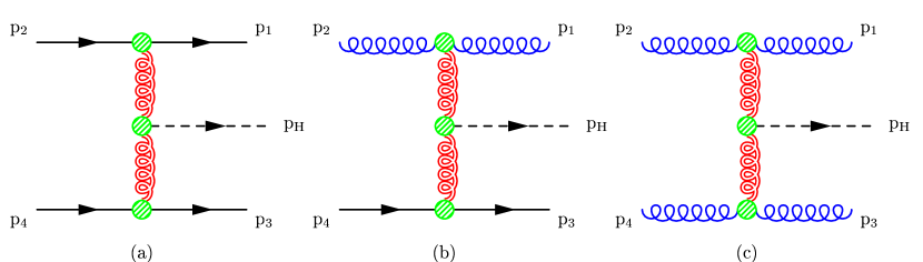
Figure 3: $(a)$ Amplitudes for $q\,Q\to q\,Q\,H$ scattering, $(b)$ for $q\,g\to q\,g\,H$ scattering and $(c)$ for $g\,g\to g\,g\,H$ scattering, in the limit (32).

For $q\,Q\to q\,Q\,H$ scattering, the amplitude, given by Eqs. (17) and (22), and illustrated by Fig. 3 (a), can be written in the high-energy limit as

$$i\ {\cal M}^{qq\to Hqq}\left(p_{2}^{-\nu_{1}},\,p_{1}^{\nu_{1}},\,p_{\scriptscriptstyle{\rm H}},\,p_{3}^{\nu_{3}},\,p_{4}^{-\nu_{3}}\right)$$ (34)

$$= 2s\left[g\,T^{c}_{a_{1}\bar{a}_{2}}\,C^{\bar{q};q}\left(p_{2}^{-\nu_{1}};p_{1}^{\nu_{1}}\right)\right]{1\over t_{1}}\left[\delta^{cc^{\prime}}C^{\scriptscriptstyle H}\left(q_{1},p_{\scriptscriptstyle{\rm H}},q_{2}\right)\right]{1\over t_{2}}\left[g\,T^{c^{\prime}}_{a_{3}\bar{a}_{4}}\,C^{\bar{q};q}\left(p_{4}^{-\nu_{3}};p_{3}^{\nu_{3}}\right)\right]\!,$$

where $q_{1}=-(p_{1}+p_{2})$, $q_{2}=p_{3}+p_{4}$, $t_{i}\simeq-|q_{i\scriptscriptstyle\perp}|^{2}$, $i=1,2$. In Eq. (34) we have made explicit the helicity conservation along the massless quark lines. The effective vertex for Higgs production along the gluon ladder, $g^{*}\,g^{*}\rightarrow H$, with $g^{*}$ an off-shell gluon (represented by the central blob in Fig. 3), is

$$C^{\scriptscriptstyle H}\left(q_{1},p_{\scriptscriptstyle{\rm H}},q_{2}\right)=2\,{g^{2}M_{t}^{2}\over v}\left[m_{\scriptscriptstyle{{\rm H}_{\perp}}}^{2}A_{1}(q_{1},q_{2})-2A_{2}(q_{1},q_{2})\right]\,,$$ (35)

with the coefficients $A_{1,2}$ defined in Eq. (81). The effective vertices $C^{\bar{q};q}$ for $g^{*}\,q\rightarrow q$ and the ones for $g^{*}\,\bar{q}\rightarrow\bar{q}$ were computed in Refs. [17, 18].

A similar analysis can be performed for $q\,g\to q\,g\,H$ scattering, Fig. 3 (b), with only the sub-amplitudes (26) and (3.2) contributing in the high-energy limit. This amplitude can also be written as Eq. (34), provided we substitute a gluon effective vertex for one of the quark effective vertices as in (11), where the gluon effective vertex, $C^{g;g}$ was computed in Ref. [15]. We have verified this analytically. The same check on the (squared) amplitude for $g\,g\to g\,g\,H$ scattering, Fig. 3 (c), has been performed numerically. Thus, in the high-energy limit the amplitudes for $q\,Q\to q\,Q\,H$, $q\,g\to q\,g\,H$ and $g\,g\to g\,g\,H$ scattering only differ by the color strength in the jet-production vertex, and it is enough to consider one of them and include the others through the effective p.d.f. (3).

Defining the coefficient function $V^{\scriptscriptstyle H}$ for $g^{*}\,g^{*}\rightarrow H$,

$$V^{\scriptscriptstyle H}\left(q_{1},p_{\scriptscriptstyle{\rm H}},q_{2}\right)=\left[\delta^{cc^{\prime}}C^{\scriptscriptstyle H}(q_{1},p_{\scriptscriptstyle{\rm H}},q_{2})\right]\left[\delta^{dd^{\prime}}\left[C^{\scriptscriptstyle H}(q_{1},p_{\scriptscriptstyle{\rm H}},q_{2})\right]^{*}\right]\,,$$ (36)

and using the impact factors for the gluon jets (5), we can write the squared amplitude $g\,g\to g\,g\,H$, summed (averaged) over final (initial) helicities and colors, as

$$\left|{\cal M}^{gg\to Hgg}\right|^{2} = 4\,s^{2}\,I^{g;g}(p_{2};p_{1})\,{1\over t_{1}^{2}}\,V^{\scriptscriptstyle H}\left(q_{1},p_{\scriptscriptstyle{\rm H}},q_{2}\right)\,{1\over t_{2}^{2}}\,I^{g;g}(p_{4};p_{3})$$ (37)

$$= 4\,{C_{A}^{2}\over N_{c}^{2}-1}\,g^{4}\,{s^{2}\over t_{1}^{2}\,t_{2}^{2}}\,\left|C^{\scriptscriptstyle H}\left(q_{1},p_{\scriptscriptstyle{\rm H}},q_{2}\right)\right|^{2}\,.$$

4.1.1 The combined high-energy limit and large top-mass limit

These scattering amplitudes can be simplified further in the large top-mass limit. Taking this limit on the coefficients $A_{1,2}$ in the vertex (35), using (82) we obtain

$$\lim_{M_{t}\to\infty}C^{\scriptscriptstyle H}\left(q_{1},p_{\scriptscriptstyle{\rm H}},q_{2}\right)=i\ {A\over 2}\left(\left|p_{\scriptscriptstyle{{\rm H}_{\perp}}}\right|^{2}-\left|q_{1\scriptscriptstyle\perp}\right|^{2}-\left|q_{2\scriptscriptstyle\perp}\right|^{2}\right)\,,$$ (38)

with the effective coupling $A$ defined in Eq. (15). Note that there is a radiation zero when the transverse momenta are at right angles to each other [22], giving the relation, $|p_{\scriptscriptstyle{{\rm H}_{\perp}}}|^{2}=|q_{1\scriptscriptstyle\perp}|^{2}+|q_{2\scriptscriptstyle\perp}|^{2}$. In the soft Higgs limit, $p_{\scriptscriptstyle{\rm H}}\to 0$, the amplitudes are proportional to those for dijet production in the high-energy limit.

We can obtain the same results by starting directly from the amplitudes for Higgs plus two partons in the large $M_{t}$ limit, given in Appendix F. It is straightforward to show that in the high-energy limit they reduce to the form of Eq. (34) (substituting gluon for quark effective vertices, where appropriate, via (11)), with the effective vertex for the Higgs given by Eq. (38). Note that only the sub-amplitude (123) for $q\,q\to q\,q\,H$ scattering, the sub-amplitudes (121) and (122) for $q\,g\to q\,g\,H$ scattering and the sub-amplitude (119) for $g\,g\to g\,g\,H$ scattering contribute in the high-energy limit, because they are the only ones to allow conservation of the quark and gluon helicities in the scattering. Thus, we again find that the two limits are interchangeable in all the sub-processes that survive in the high-energy limit (32).

4.2 The high-energy limit $\boldsymbol{s_{j_{1}j_{2}},\,s_{j_{2}\scriptscriptstyle{\rm H}}\gg s_{j_{1}\scriptscriptstyle{\rm H}},\,M_{\scriptscriptstyle{\rm H}}^{2}}$

Next, we consider the limit in which the Higgs boson is produced forward in rapidity, and close to one of the jets, say to jet $j_{1}$, and both are very far from jet $j_{2}$, i.e. $s_{j_{1}j_{2}},\,s_{j_{2}\scriptscriptstyle{\rm H}}\gg s_{j_{1}\scriptscriptstyle{\rm H}},\,M_{\scriptscriptstyle{\rm H}}^{2}$. Labeling the partons as in the previous section, we find that this limit implies

$$p_{1}^{+}\simeq p_{\scriptscriptstyle{\rm H}}^{+}\gg p_{3}^{+}\,,\qquad p_{1}^{-}\simeq p_{\scriptscriptstyle{\rm H}}^{-}\ll p_{3}^{-}\,.$$ (39)

In this limit, the amplitudes are again dominated by gluon exchange in the $t$ channel, and factorize into an effective vertex for the production of a jet and another for the production of a Higgs plus a jet.

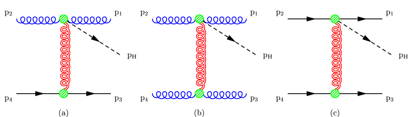
Figure 4: $(a)$ Amplitudes for $q\,g\to q\,H\,g$ scattering, $(b)$ for $g\,g\to g\,H\,g$ scattering, and $(c)$ for $q\,q\to q\,H\,q$ scattering, in the limit (39).

We consider first the amplitude for $q\,g\to q\,g\,H$ scattering with the incoming gluon (quark) of momentum $p_{2}$ ($p_{4}$), as in Fig. 4 (a). In this case all of the sub-amplitudes (26)–(28) are leading, and to the required accuracy the sub-amplitude (3.2) is equal and opposite to Eq. (26). Then the amplitude for $q\,g\to q\,g\,H$ scattering can be written as

$$i\ {\cal M}^{gq\to gHq}\left(p_{2}^{\nu_{2}},\,p_{1}^{\nu_{1}},\,p_{\scriptscriptstyle{\rm H}},\,p_{3}^{\nu_{3}},\,p_{4}^{-\nu_{3}}\right)$$aaaaaa (40)

$$= 2\,s\left[ig\,f^{a_{2}a_{1}c}\,C^{g;{\scriptscriptstyle H}g}\left(p_{2}^{\nu_{2}};p_{1}^{\nu_{1}},p_{\scriptscriptstyle{\rm H}}\right)\right]{1\over t}\left[ig\,T^{c}_{a_{3}\bar{a}_{4}}\,C^{\bar{q};q}\left(p_{4}^{-\nu_{3}};p_{3}^{\nu_{3}}\right)\right]\,,$$

where the effective vertex for the production of a quark jet $C^{\bar{q};q}$ was computed in Refs. [17, 18], and where $C^{g;{\scriptscriptstyle H}g}(p_{2}^{\nu_{2}};p_{1}^{\nu_{1}},p_{\scriptscriptstyle{\rm H}})$ is the effective vertex for the production of a Higgs boson and a gluon jet, $g^{*}g\to gH$ (the upper blob in Fig. 4 (a) and (b)). In Eq. (40) the momentum transfer is $t=q^{2}\simeq-|q_{\scriptscriptstyle\perp}|^{2}$, with $q=p_{3}+p_{4}$. There are two distinct helicity configurations for the effective vertex $C^{g;{\scriptscriptstyle H}g}$ that contribute. For the helicity-conserving configuration we find

$$C^{g;{\scriptscriptstyle H}g}(p_{2}^{-};p_{1}^{+},p_{\scriptscriptstyle{\rm H}})=-i{g^{4}M_{t}^{2}\over\ v}\,\frac{1}{4s_{12}}\ \frac{1}{s^{2}}\sqrt{1+{p_{\scriptscriptstyle{\rm H}}^{+}\over p_{1}^{+}}}$$aaaaaa (41)

$$\Bigl{\{}\Bigl{(}\langle 2|3|1\rangle+\langle 2|4|1\rangle\Bigr{)}\Bigl{[}(s_{13})^{2}\Bigl{(}8A_{1}(1;234)-2S_{2}H_{12}\Bigr{)}$$

$$\qquad+(s_{24})^{2}\Bigl{(}-8A_{1}(2;134)-2S_{1}H_{10}\Bigr{)}$$

$$\qquad+s_{13}s_{24}\Bigl{(}4(H_{4}+H_{5})+2S_{2}H_{10}+2S_{1}H_{12}\Bigr{)}\Bigr{]}$$

$$+\Bigl{(}\langle 2|3|1\rangle-\langle 2|4|1\rangle\Bigr{)}\Bigl{[}s_{13}\Bigl{(}-\Delta H_{12}-4S_{1}A_{1}(1;234)\Bigr{)}$$

$$\qquad+s_{24}\Bigl{(}\Delta H_{10}-4S_{2}A_{1}(2;134)\Bigr{)}\Bigr{]}\Bigr{\}}\,,$$

with invariants given in Eq. (107), and currents in Eq. (104). For the sake of compactness, we have relegated the necessary sub-formulae, along with some details of the derivation, to Appendix E. Note that since the term in curly brackets is ${\cal O}(s^{2})$, Eq. (41) is manifestly ${\cal O}(s^{0})$.

For the helicity-nonconserving configuration we find

$$C^{g;{\scriptscriptstyle H}g}(p_{2}^{+};p_{1}^{+},p_{\scriptscriptstyle{\rm H}}) = -i\ {g^{4}M_{t}^{2}\over\ v}\,\frac{1}{2s_{12}}\ {1\over s}\ {p_{1_{\perp}}^{*}\over p_{1_{\perp}}}{p_{3_{\perp}}\over|p_{3_{\perp}}|}$$ (42)

$$\biggl{\{}-\langle 4|1|3\rangle\ (2s_{12}H_{1}+\Delta H_{12})-\langle 4|2|3\rangle\ (2s_{12}H_{2}+\Delta H_{10})$$

$$\quad+2\left(\langle 4|1|3\rangle s_{24}+\langle 4|2|3\rangle s_{13}\right)\ H_{4}$$

$$\quad+2\bigl{[}\langle 4|1|3\rangle S_{2}+\langle 4|2|3\rangle S_{1}-(\langle 4|1|3\rangle s_{24}+\langle 4|2|3\rangle s_{13})\bigr{]}\ H_{5}$$

$$+{4\over s_{13}s_{2{\rm H}}}\biggl{[}\left[s_{13}(2s_{12}+S_{2})-s_{24}s_{34}\right](\langle 4|1|3\rangle s_{24}+\langle 4|2|3\rangle s_{13})$$

$$\qquad+\left[2s_{24}s_{34}(s_{12}+S_{2})-s_{13}(s_{12}+S_{2})^{2}\right]\ \langle 4|1|3\rangle$$

$$\qquad+s_{13}(s_{34}S_{2}-s_{12}S_{1})\langle 4|2|3\rangle\biggr{]}A_{1}(2;134)$$

$$+{4\over s_{24}s_{1{\rm H}}}\biggl{[}\left[s_{24}(2s_{12}+S_{1})-s_{13}s_{34}\right](\langle 4|1|3\rangle s_{24}+\langle 4|2|3\rangle s_{13})$$

$$\qquad+\bigl{[}s_{24}\left[s_{12}s_{34}+(s_{12}+S_{1})(s_{34}-S_{2})\right]+s_{13}s_{34}S_{2}\bigr{]}\ \langle 4|1|3\rangle$$

$$\qquad+\left(s_{13}s_{34}S_{1}+s_{24}s_{12}^{2}\right)\langle 4|2|3\rangle\biggr{]}A_{1}(1;234)$$

$$+2(S_{1}-S_{2})\ (\langle 4|1|3\rangle+\langle 4|2|3\rangle)\ A_{1}(12;34)$$

$$-4(\langle 4|1|3\rangle-\langle 4|2|3\rangle)\ A_{2}(12;34)\biggr{\}},$$

with invariants given in Eq. (107), and currents in Eqs. (108) and (109). The term in curly brackets in Eq. (42) is ${\cal O}(s)$, and thus this effective vertex is ${\cal O}(s^{0})$. Finally, note that Eqs. (41) and (42) transform under parity into their complex conjugates

$$[C^{g;{\scriptscriptstyle H}g}(\{k^{\nu}\})]^{*}=C^{g;{\scriptscriptstyle H}g}(\{k^{-\nu}\})\,.$$ (43)

As in Eq. (5), we define the impact factor for the production of a Higgs and a gluon jet, summed (averaged) over final (initial) helicities and colors, as

$$I^{g;{\scriptscriptstyle H}g}\left(p_{2};p_{1},p_{\scriptscriptstyle{\rm H}}\right)$$ (44)

$$= \frac{1}{2(N_{c}^{2}-1)}\left[ig\,f^{a_{2}a_{1}c}\,C^{g;{\scriptscriptstyle H}g}\left(p_{2}^{\nu_{2}};p_{1}^{\nu_{1}},p_{\scriptscriptstyle{\rm H}}\right)\right]\left[-ig\,f^{a_{2}a_{1}d}\,\left[C^{g;{\scriptscriptstyle H}g}\left(p_{2}^{\nu_{2}};p_{1}^{\nu_{1}},p_{\scriptscriptstyle{\rm H}}\right)\right]^{*}\right]$$

$$= g^{2}\,{C_{A}\over N_{c}^{2}-1}\,\delta^{cd}\ \left[\left|C^{g;{\scriptscriptstyle H}g}\left(p_{2}^{-};p_{1}^{+},p_{\scriptscriptstyle{\rm H}}\right)\right|^{2}+\left|C^{g;{\scriptscriptstyle H}g}\left(p_{2}^{+};p_{1}^{+},p_{\scriptscriptstyle{\rm H}}\right)\right|^{2}\right]\,,$$

where in the first line a sum over repeated indices is implicit. Finally, the squared amplitude, summed (averaged) over final (initial) helicities and colors is

$$\left|{\cal M}^{gq\to gHq}\right|^{2}={4s^{2}\over t^{2}}\,I^{g;{\scriptscriptstyle H}g}\left(p_{2};p_{1},p_{\scriptscriptstyle{\rm H}}\right)\,I^{{\bar{q}};q}\left(p_{4};p_{3}\right)\,,$$ (45)

with the impact factor for the quark jet given by Eq. (12). High-energy factorization implies that the amplitude for $g\,g\to g\,g\,H$ scattering, Fig. 4 (b), also can be put in the form (40), up to the replacement of the incoming quark with a gluon via the substitution (11).

The amplitude for $q\,Q\to q\,Q\,H$ scattering, Fig. 4 (c), factorizes into an effective vertex for the production of a Higgs and a quark jet, $g^{*}q\to qH$, and the effective vertex for the production of a quark jet only. Using Eqs. (17) and (22), it can be written as

$$i\ {\cal M}^{qQ\to qHQ}\left(p_{2}^{-\nu_{1}},\,p_{1}^{\nu_{1}},\,p_{\scriptscriptstyle{\rm H}},\,p_{3}^{\nu_{3}},\,p_{4}^{-\nu_{3}}\right)$$aaaaa (46)

$$= 2s\left[g\,T^{c}_{a_{1}\bar{a}_{2}}\,C^{\bar{q};{\scriptscriptstyle H}q}\left(p_{2}^{-\nu_{1}};p_{1}^{\nu_{1}},p_{\scriptscriptstyle{\rm H}}\right)\right]{1\over t}\left[g\,T^{c}_{a_{3}\bar{a}_{4}}\,C^{\bar{q};q}\left(p_{4}^{-\nu_{3}};p_{3}^{\nu_{3}}\right)\right]\,,$$

with the vertex for the production of a quark jet, $C^{\bar{q};q}$, computed in Refs. [17, 18], and the vertex $g^{*}q\to q\,H$ (the upper blob in Fig. 4 (c)) given by

$$C^{\bar{q};{\scriptscriptstyle H}q}\left(p_{2}^{-};p_{1}^{+},p_{\scriptscriptstyle{\rm H}}\right) = -2i\ {g^{2}M_{t}^{2}\over v}{1\over s_{12}}\ \left(1+{p_{\scriptscriptstyle{\rm H}}^{+}\over p_{1}^{+}}\right)^{-1/2}$$ (47)

$$\times \left\{\left[m_{\scriptscriptstyle{{\rm H}_{\perp}}}^{2}+{p_{\scriptscriptstyle{\rm H}}^{+}\over p_{1}^{+}}\left(|p_{1_{\perp}}|^{2}+p_{1_{\perp}}^{*}q_{{}_{\perp}}\right)\right]A_{1}(q_{1},q_{2})-2A_{2}(q_{1},q_{2})\right\},\phantom{aaa}$$

with coefficients $A_{1,2}$ defined in Eq. (81). Note that in the more restrictive limit (32), where the Higgs is also separated by a large rapidity interval from jet $j_{1}$, this vertex factorizes further into an effective vertex for the production of the Higgs along the ladder, Eq. (35), a gluon propagator $1/s_{12}$, and an effective vertex for the production of a quark jet, $C^{\bar{q};q}(p_{2};p_{1})$. Finally, note that under parity Eq. (47) transforms into its complex conjugate and changes sign,

$$[C^{{\bar{q}};{\scriptscriptstyle H}q}(\{k^{\nu}\})]^{*}=-C^{{\bar{q}};{\scriptscriptstyle H}q}(\{k^{-\nu}\})\,.$$ (48)

The impact factor for the production of a Higgs and a quark jet is given by

$$I^{\bar{q};{\scriptscriptstyle H}q}\left(p_{2};p_{1},p_{\scriptscriptstyle{\rm H}}\right) = {1\over 2N_{c}}\left[g\,T^{c}_{a_{1}\bar{a}_{2}}\,C^{\bar{q};{\scriptscriptstyle H}q}\left(p_{2}^{\nu_{2}};p_{1}^{\nu_{1}},p_{\scriptscriptstyle{\rm H}}\right)\right]\left[g\,T^{d}_{\bar{a}_{2}a_{1}}\,\left[C^{\bar{q};{\scriptscriptstyle H}q}\left(p_{2}^{\nu_{2}};p_{1}^{\nu_{1}},p_{\scriptscriptstyle{\rm H}}\right)\right]^{*}\right]$$ (49)

$$= g^{2}\ {1\over 2N_{c}}\ \delta^{cd}\left|C^{\bar{q};{\scriptscriptstyle H}q}\left(p_{2}^{-};p_{1}^{+},p_{\scriptscriptstyle{\rm H}}\right)\right|^{2}\ ,$$

with $\nu_{2}=-\nu_{1}$, and an implicit sum over repeated indices. Thus the squared amplitude for $q\,Q\to q\,H\,Q$ scattering, summed (averaged) over final (initial) helicities and colors, is

$$\left|{\cal M}^{qQ\to qHQ}\right|^{2}={4s^{2}\over t^{2}}\,I^{{\bar{q}};{\scriptscriptstyle H}q}\left(p_{2};p_{1},p_{\scriptscriptstyle{\rm H}}\right)\,I^{{\bar{q}};q}\left(p_{4};p_{3}\right)\,,$$ (50)

with the impact factor for the quark jet given by Eq. (12).

4.2.1 The combined high-energy limit and large top-mass limit

In the large top-mass limit, the amplitude for $q\,Q\to q\,Q\,H$ scattering (46) can be simplified further by using the limits (82) for the coefficients $A_{1,2}$. The effective vertex for the production of a Higgs and a quark jet (47) reduces to

$$\lim_{M_{t}\to\infty}C^{\bar{q};{\scriptscriptstyle H}q}\left(p_{2}^{-};p_{1}^{+},p_{\scriptscriptstyle{\rm H}}\right)={A\over 2}{1\over s_{12}}\ \left(1+{p_{\scriptscriptstyle{\rm H}}^{+}\over p_{1}^{+}}\right)^{-1/2}\left[p_{1_{\perp}}p_{3_{\perp}}^{*}+\left(1+{p_{\scriptscriptstyle{\rm H}}^{+}\over p_{1}^{+}}\right)p_{1_{\perp}}^{*}p_{3_{\perp}}\right]\ .$$ (51)

Again we note that in the limit (32), for which the Higgs is separated by a large rapidity interval from jet $j_{1}$, Eq. (51) factorizes into the effective vertex for the production of the Higgs along the ladder in the large $M_{t}$ limit, Eq. (38), a gluon propagator $1/s_{12}$, and an effective vertex for the production of a quark jet, $C^{\bar{q};q}(p_{2};p_{1})$. Conversely, this vertex (51) can be derived by taking the limit (39) on the amplitude for Higgs plus two $q\bar{q}$ pairs (123) in the large $M_{t}$ limit.

Given the algebraic complexity of Eqs. (41) and (42), it is easier to derive the large $M_{t}$ limit of the effective vertex for the production of a Higgs and a gluon jet by directly taking the limit (39) on the large $M_{t}$ amplitudes for $q\,g\to q\,g\,H$ scattering. Thus, from Eqs. (121) and (122) we obtain the helicity-conserving configuration

$$\lim_{M_{t}\to\infty}C^{g;{\scriptscriptstyle H}g}(p_{2}^{-};p_{1}^{+},p_{\scriptscriptstyle{\rm H}})=i\,{A\over 2}{1\over s_{12}}\ \left(1+{p_{\scriptscriptstyle{\rm H}}^{+}\over p_{1}^{+}}\right)^{-1}\left[p_{1_{\perp}}p_{3_{\perp}}^{*}+\left(1+{p_{\scriptscriptstyle{\rm H}}^{+}\over p_{1}^{+}}\right)^{2}p_{1_{\perp}}^{*}p_{3_{\perp}}\right]\ .$$ (52)

We have verified that we obtain the same result by taking the limit (39) on the amplitudes for $g\,g\to g\,g\,H$ scattering, Eq. (119). From Eq. (120) we obtain the helicity-nonconserving configuration

$$\lim_{M_{t}\to\infty}C^{g;{\scriptscriptstyle H}g}\left(p_{2}^{+};p_{1}^{+},p_{\scriptscriptstyle{\rm H}}\right)=-i\,{A\over 2}{1\over s_{12}}\left\{p_{1_{\perp}}^{*}p_{3_{\perp}}^{*}\left({p_{\scriptscriptstyle{\rm H}}^{+}\over p_{1}^{+}}\right)^{2}\left(1+{p_{\scriptscriptstyle{\rm H}}^{+}\over p_{1}^{+}}\right)^{-1}\right.$$

$$\left.+\left[{(p_{\scriptscriptstyle{{\rm H}_{\perp}}}^{*})^{2}\over|p_{\scriptscriptstyle{{\rm H}_{\perp}}}|^{2}+p_{1}^{+}p_{\scriptscriptstyle{\rm H}}^{-}}-\left(1+{p_{\scriptscriptstyle{\rm H}}^{+}\over p_{1}^{+}}\right)^{-1}\frac{1}{M_{\scriptscriptstyle{\rm H}}^{2}+2p_{1}\cdot p_{\scriptscriptstyle{\rm H}}}\left[p_{3_{\perp}}^{*}+\left(1+{p_{\scriptscriptstyle{\rm H}}^{+}\over p_{1}^{+}}\right)p_{1_{\perp}}^{*}\right]^{2}\right]s_{12}\right\}\ .$$

In the more restrictive limit (32), Eq. (4.2.1) is subleading as expected, while Eq. (52) factorizes further into the effective vertex for the production of the Higgs along the ladder in the large $M_{t}$ limit, Eq. (38), a gluon propagator $1/s_{12}$, and an effective vertex for the production of a gluon jet, $C^{g;g}(p_{2};p_{1})$.

4.3 The production rate for Higgs + 2 jets

Using the formulae for the squared matrix elements, given in the previous sections, one can compute the cross section for Higgs boson production in association with two jets, in either of the two high-energy limits. In the numerical work in this section, we focus on the more restrictive limit (32), where the Higgs boson is central in the rapidity interval and widely separated from both of the two jets.

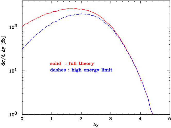
Figure 5: Cross section in $H+2$ jet production in $pp$ collisions at the LHC energy $\sqrt{s}=14$ TeV as a function of $\Delta y$, with $M_{\scriptscriptstyle{\rm H}}=120$ GeV and $M_{t}=175$ GeV. The dijet invariant mass fulfils the constraint $\sqrt{s_{j_{1}j_{2}}}\geq 600$ GeV. The rapidity interval $\Delta y$ is defined as $\Delta y={\rm min}(|y_{j_{1}}-y_{\scriptscriptstyle{\rm H}}|,|y_{j_{2}}-y_{\scriptscriptstyle{\rm H}}|)$, with the kinematical constraint $y_{j_{1}}>y_{\scriptscriptstyle{\rm H}}>y_{j_{2}}$. The solid line represents the exact production rate; the dashed line the rate in the high-energy limit.

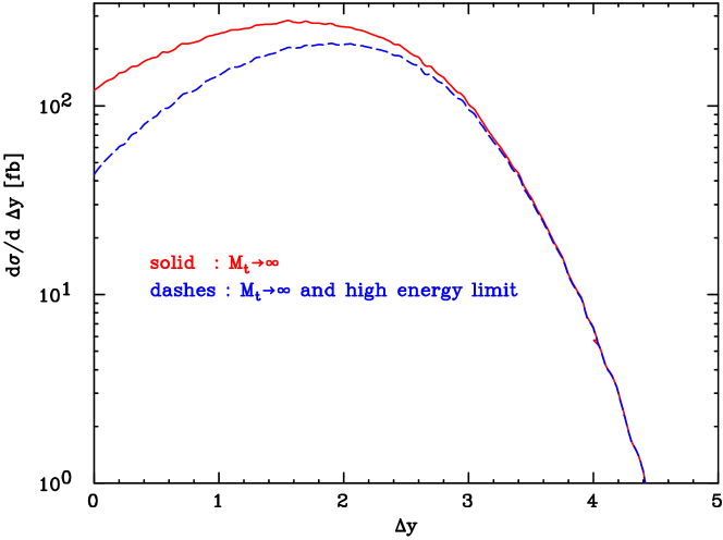
Figure 6: Same as Fig. 5, with the solid line representing the production rate in the large $M_{t}$ limit, and the dashed line the rate in the combined large $M_{t}$ plus high-energy limit.

In Figs. 5 and 6 we plot the cross section for $H+2$ jet production in $pp$ collisions at the LHC energy $\sqrt{s}=14$ TeV, as a function of $\Delta y$, where $\Delta y={\rm min}(|y_{j_{1}}-y_{\scriptscriptstyle{\rm H}}|,|y_{j_{2}}-y_{\scriptscriptstyle{\rm H}}|)$, with the kinematical constraint $y_{j_{1}}>y_{\scriptscriptstyle{\rm H}}>y_{j_{2}}$. That is, $\Delta y$ is defined as the smallest rapidity difference among the final-state particles. In addition we have imposed the following set of cuts

$$|p_{j_{\perp}}|>20\;{\rm GeV},\quad|y_{j_{1,2}}|<5,\quad y_{j_{1}}y_{j_{2}}<0,\quad\sqrt{s_{j_{1}j_{2}}}\geq 600~{}{\rm GeV},\quad R_{jj}>0.6$$ (54)

where $R_{jj}$ describes the separation of the two partons in the rapidity $y$ versus azimuthal angle plane

$$R_{jj}=\sqrt{\Delta y_{jj}^{2}+\Delta\phi_{jj}^{2}}\;.$$ (55)

In the plots we used values of the Higgs and top-quark masses of $M_{\scriptscriptstyle{\rm H}}=120$ GeV and $M_{t}=175$ GeV, respectively. A fixed value of $\alpha_{\scriptscriptstyle S}=0.12$ has been chosen, and the factorization scale has been taken to be $\mu_{\scriptscriptstyle{\rm F}}=\sqrt{p_{j_{1\perp}}p_{j_{2\perp}}}$. The leading order p.d.f.’s of the CTEQ4L package [23] have been used. In Fig. 5 the solid line represents the production rate with the exact amplitudes, as evaluated in Ref. [5], and the dashed line represents the rate in the high-energy limit (i.e., using the squared matrix element of (37) with the effective p.d.f. (3)); in Fig. 6 the solid line represents the production rate with the amplitudes evaluated in the large $M_{t}$ limit (given in Appendix F.3), and the dashed line the rate in the combined large $M_{t}$ plus high-energy limit from Section 4.1.1.

In Figs. 5 and 6, the agreement between the curves is very good for $\Delta y\gtrsim 3$. The agreement for $\Delta y\lesssim 3$, where the high-energy limit is not expected to be a good approximation, depends on the exact details of how the high-energy limit is taken. In calculating the dashed curve of Fig. 5, we took the coefficients $A_{1,2}$ of Eq. (35) to be a function of $q_{1}^{2}$ and $q_{2}^{2}$ evaluated in the high-energy limit, i.e., $q_{1}^{2}=-q_{1\perp}^{2}$ and $q_{2}^{2}=-q_{2\perp}^{2}$; however, in Eq. (34) we evaluated the gluon propagators $t_{1}$ and $t_{2}$ at the exact values $q_{1}^{2}$ and $q_{2}^{2}$. This choice makes the high-energy limit curve of Fig. 5 (and respectively the combined limit curve of Fig. 6) converge faster to the exact curve (to the large $M_{t}$ limit curve) than using $t_{1}=-q_{1\perp}^{2}$ and $t_{2}=-q_{2\perp}^{2}$. Of course, either choice for the value of the gluon propagators is equally valid in the high-energy limit. We can only ascertain a posteriori which gives a better numerical agreement with the exact calculation at finite $\Delta y$.

5 Conclusions

In this paper we have analyzed the high-energy limit for Higgs boson plus one and two jet production. For Higgs boson plus two jet production we considered two versions of the high-energy limit, corresponding to two different kinematic regions: (a) $s_{j_{1}j_{2}}\gg s_{j_{1}\scriptscriptstyle{\rm H}},s_{j_{2}\scriptscriptstyle{\rm H}}\gg M_{\scriptscriptstyle{\rm H}}^{2}$, i.e. the Higgs boson is centrally located in rapidity between the two jets, and very far from either jet; (b) $s_{j_{1}j_{2}},s_{j_{2}\scriptscriptstyle{\rm H}}\gg s_{j_{1}\scriptscriptstyle{\rm H}},M_{\scriptscriptstyle{\rm H}}^{2}$, i.e. the Higgs boson is close to jet $j_{1}$ in rapidity, and both of these are very far from jet $j_{2}$. In all cases the amplitudes factorize into impact factors or coefficient functions connected by gluons exchanged in the $t$ channel. We obtained the relevant impact factors, keeping the full $M_{t}$ dependence, for all of the partonic subprocesses which contribute in the high-energy limits. In particular, we computed the impact factor for the production of a Higgs boson (8) from the high-energy limit of Higgs $+$ one jet production; the coefficient function for the production of a Higgs from two off-shell gluons (36) from case (a) in Higgs $+$ two jet production; and the impact factors for the production of a Higgs in association with a gluon (44) or a quark  (49) jet from case (b) in Higgs $+$ two jet production. This required the full one-loop $M_{t}$-dependent $q\,Q\to q\,Q\,H$ and $g\,q\to g\,q\,H$ amplitudes, which we have presented here in a new form, which is convenient for our purposes.

In addition, we have investigated the interplay of the high-energy limit with that of the large $M_{t}$ limit. We have computed the same impact factors and coefficient functions as above, but also in the large $M_{t}$ limit, and we have shown that the imposition of the two different limits commutes. This is important, because it implies that the factorization of amplitudes at high energies ensures that the large $M_{t}$ computations are not made invalid by the presence of an overall large energy scale, as long as the typical transverse energy scale is less than or of the order of the top mass. This effect was first noted in Ref. [5], where we ascertained that for Higgs $+$ two jet production the necessary conditions to use the large $M_{t}$ limit are that the Higgs mass is smaller than the threshold for the creation of a top-quark pair, $M_{\scriptscriptstyle{\rm H}}\lesssim 2M_{t}$ and the jet transverse energies are smaller than the top-quark mass, $p_{{}\scriptscriptstyle\perp}\lesssim M_{t}$. However, the size of the dijet invariant mass was irrelevant to the applicability of the large $M_{t}$ limit.

In general, the calculation of Higgs production via gluon-gluon fusion in association with one or more jets is quite complicated, even at lowest order in $\alpha_{\scriptscriptstyle S}$, because in this process the Higgs boson is produced via a heavy quark loop. In Higgs $+$ one jet production, triangle and box loops occur; in Higgs $+$ two jet production, pentagon loops also occur, and in Higgs $+\ n$ jet production, up to $(n+3)$–side polygon quark loops occur. In Ref. [5] we computed Higgs $+$ two jet production, but the complexity of the calculation discourages one from carrying on this path. For instance, the evaluation of the radiative corrections at ${\cal O}(\alpha_{\scriptscriptstyle S})$ to Higgs $+$ two jet production would imply the calculation of up to hexagon quark loops and two-loop pentagon quark loops, which are at present unfeasible. Fortunately, there are two types of limits in which the calculations become simpler:

• the large $M_{t}$ limit, in which the heavy quark loop is replaced by an effective coupling, thus reducing the number of loops in a given diagram by one;

• the high-energy limits, in which the number of sides in the largest polygon quark loop is diminished at least by one.

We have seen that both of these limits can be relevant to phenomenology and they can give useful and complementary information, both as cross checks of an exact calculation with the full $M_{t}$ dependence, and as the starting point for a more detailed calculation in which a well-based simplifying assumption is crucial.

Appendix A Scalar integrals

We define the scalar integrals by

$$B_{0}(k) = \int\kern-5.0pt{d^{n}\!q\over(2\pi)^{n}}{1\over\left(q^{2}-M_{t}^{2}\right)\left[(q+k)^{2}-M_{t}^{2}\right]}-\frac{i}{16\pi^{2}}\left(4\pi\right)^{\epsilon}M_{t}^{-2\epsilon}\frac{\Gamma(1+\epsilon)}{\epsilon}$$ (56)

$$C_{0}(p;k) = \int\kern-5.0pt{d^{4}\!q\over(2\pi)^{4}}{1\over\left(q^{2}-M_{t}^{2}\right)\left[(q+p)^{2}-M_{t}^{2}\right]\left[(q+p+k)^{2}-M_{t}^{2}\right]}$$ (57)

$$D_{0}(p;k;v) = \int\kern-5.0pt{d^{4}\!q\over(2\pi)^{4}}\left\{\frac{1}{\left(q^{2}-M_{t}^{2}\right)\left[(q+p)^{2}-M_{t}^{2}\right]\left[(q+p+k)^{2}-M_{t}^{2}\right]}\right.$$ (58)

$$\qquad\qquad\qquad\times\left.\frac{1}{\left[(q+p+k+v)^{2}-M_{t}^{2}\right]}\right\}\ .$$

The arguments of the left-hand side label the momenta of the propagators in successive order. Note that the scalar integrals are invariant under inversion of the order of the momenta; e.g. $D_{0}(p;k;v)=D_{0}(v;k;p)$. The integrals $C_{0}$ and $D_{0}$ are expressly finite in four dimensions, while the integral $B_{0}$ only occurs in combinations that are finite as $\epsilon\equiv(4-n)/2\rightarrow 0$. Therefore, we have explicitly removed the $1/\epsilon$-pole from its definition.

Explicit formulae for some of the scalar integrals are

(67)

where

$$Q = -q_{1}-q_{2}$$

and

$$\Delta_{3} = (q_{1}^{2})^{2}+(q_{2}^{2})^{2}+(Q^{2})^{2}-2q_{1}^{2}q_{2}^{2}-2q_{1}^{2}Q^{2}-2q_{2}^{2}Q^{2}$$

$$\delta_{1}={q_{1}^{2}-q_{2}^{2}-Q^{2}\over\sqrt{\Delta_{3}}}\ ,\qquad\delta_{2}={-q_{1}^{2}+q_{2}^{2}-Q^{2}\over\sqrt{\Delta_{3}}}\ ,\qquad\delta_{3}={-q_{1}^{2}-q_{2}^{2}+Q^{2}\over\sqrt{\Delta_{3}}}\ ,$$ (68)

$$\delta_{1}^{+}=\frac{1+\delta_{1}}{2},\quad\delta_{2}^{+}=\frac{1+\delta_{2}}{2},\quad\delta_{3}^{+}=\frac{1+\delta_{3}}{2},$$ (69)

$$\delta_{1}^{-}=\frac{1-\delta_{1}}{2},\quad\delta_{2}^{-}=\frac{1-\delta_{2}}{2},\quad\delta_{3}^{-}=\frac{1-\delta_{3}}{2},$$ (70)

$$x_{\pm} = {q_{2}^{2}\over 2M_{t}^{2}}\pm{q_{2}^{2}\over 2M_{t}^{2}}\sqrt{1-{4M_{t}^{2}\over q_{2}^{2}}}\ ,\quad y_{\pm}={q_{1}^{2}\over 2M_{t}^{2}}\pm{q_{1}^{2}\over 2M_{t}^{2}}\sqrt{1-{4M_{t}^{2}\over q_{1}^{2}}}\ ,$$

$$z_{\pm} = {Q^{2}\over 2M_{t}^{2}}\pm{Q^{2}\over 2M_{t}^{2}}\sqrt{1-{4M_{t}^{2}\over Q^{2}}}$$ (71)

Appendix B The top triangle with two off-shell gluons

The triangle vertex for two off-shell gluons of momenta $q_{1}^{\mu}$ and $q_{2}^{\nu}$ and color indexes $a$ and $b$ respectively, and a Higgs boson of momentum $Q$, with $q_{1}+q_{2}+Q=0$ is given by

$${\cal A}^{\mu\nu}=4\,\delta^{ab}\,{g^{2}M_{t}^{2}\over\ v}\Bigl{[}q_{2}^{\mu}q_{1}^{\nu}A_{1}(q_{1};q_{2})-g^{\mu\nu}A_{2}(q_{1};q_{2})\Bigr{]}\,,$$ (72)

where we have dropped all terms proportional to $q_{1}^{\mu}$ and $q_{2}^{\nu}$, since they are contracted with external conserved currents, and with

(81)

with the scalar integrals evaluated in Appendix A. In the infinite top-mass limit (111), the coefficients $A_{1,2}$ become

$$\lim_{M_{t}\to\infty}4\,{g^{2}M_{t}^{2}\over\ v}\,A_{1}=iA\qquad\qquad\lim_{M_{t}\to\infty}4\,{g^{2}M_{t}^{2}\over\ v}\,A_{2}=i\,q_{1}\cdot q_{2}A\,.$$ (82)

where $A$ is given in Eq. (15).

Appendix C The top box diagram with one off-shell gluon

There are three distinct box diagrams (including both directions of fermion flow) with two on-shell gluons with momenta $k_{1}^{\mu}$ and $k_{2}^{\nu}$ and color indexes $a$ and $b$, one off-shell gluon with momentum $k^{\rho}\equiv k_{3}^{\rho}+k_{4}^{\rho}$ and color index $c$, and a Higgs boson of momentum $k_{H}$, with $k_{1}+k_{2}+k+k_{H}=0$. The sum of the three box diagrams can be parametrized in terms of 14 form factors $H_{i}$ by

$${\cal M}^{\mu\nu\rho}\ =\ {g^{3}M_{t}^{2}\over v}\,2\,if^{bac}\,J^{\mu\nu\rho}$$ (83)

with

$$J^{\mu\nu\rho} = g^{\mu\nu}\left(H_{1}\ k_{1}^{\rho}+H_{2}\ k_{2}^{\rho}\right)+g^{\mu\rho}\left(H_{3}\ k_{1}^{\nu}+H_{4}\ k^{\nu}\right)+g^{\nu\rho}\left(H_{5}\ k^{\mu}+H_{6}\ k_{2}^{\mu}\right)$$

$$+ H_{7}\ k_{1}^{\nu}k_{2}^{\mu}k_{2}^{\rho}+H_{8}\ k^{\nu}k_{2}^{\mu}k_{2}^{\rho}+H_{9}\ k_{2}^{\mu}k_{1}^{\nu}k_{1}^{\rho}+H_{10}\ k_{2}^{\rho}k^{\mu}k^{\nu}$$

$$+ H_{11}\ k^{\mu}k_{1}^{\nu}k_{1}^{\rho}+H_{12}\ k_{1}^{\rho}k^{\mu}k^{\nu}+H_{13}\ k_{2}^{\mu}k_{1}^{\rho}k^{\nu}+H_{14}\ k^{\mu}k_{1}^{\nu}k_{2}^{\rho}\ ,$$

where we have removed terms with $k_{1}^{\mu}$, $k_{2}^{\nu}$, and $k^{\rho}$, using the fact that the contraction with the respective polarization vector is zero ($k_{i}\cdot\epsilon(k_{i})=0$) and that the off-shell gluon is going to be contracted with an on-shell fermion or gluon current.

As discussed in Section 3.2, we can express the amplitudes for $q\,g\to q\,g\,H$ scattering in terms of just 6 of the form factors: $H_{1},H_{2},H_{4},H_{5},H_{10},H_{12}$. In addition, these are related by

$$H_{2} = -H_{1}\{k_{1}\leftrightarrow k_{2}\}$$

$$H_{5} = -H_{4}\{k_{1}\leftrightarrow k_{2}\}$$ (85)

$$H_{12} = -H_{10}\{k_{1}\leftrightarrow k_{2}\}\ .$$

In the interest of brevity we will therefore only give the expressions for $H_{1},H_{4},H_{10}$.

We write the form factors as the sum of the contributions from the three distinct gluon orderings in the box diagram, $H_{i}=E_{i}+F_{i}+G_{i}$. They are functions of the scalar integrals, $B_{0}(q)$, $C_{0}(q;p)$, and $D_{0}(q;p;k)$, defined in Appendix A, and are related to the box form factors of Appendix D of Ref. [5]. For notational convenience we write the arguments of the scalar integrals by the number of the parton momentum, combining numbers if the momenta are added: e.g. $C_{0}(12;34)\equiv C_{0}(k_{1}+k_{2};\,k_{3}+k_{4})$. The coefficients of the scalar integrals are functions of four variables $s_{12},s_{34},S_{1},S_{2}$ with

$$s_{ij} = (k_{i}+k_{j})^{2}$$

$$S_{i} = 2\,k_{i}\cdot k\ =\ s_{i3}+s_{i4}\ .$$ (86)

To simplify the expressions we also find it useful to introduce the following variables, which arise as determinants in the Passarino-Veltman reduction [24],

$$\Delta = s_{12}s_{34}-S_{1}S_{2}$$ (87)

$$\Sigma = 4s_{12}s_{34}-(S_{1}+S_{2})^{2}\ .$$

In terms of these variables we obtain

$$E_{1} = -s_{12}D_{0}(2;1;34)\Biggl{[}1-\frac{8M_{t}^{2}}{s_{12}}+\frac{S_{2}}{2s_{12}}+\frac{S_{2}(s_{12}-8M_{t}^{2})(s_{34}+S_{1})}{2s_{12}\Delta}$$

$$\qquad\qquad+\frac{2(s_{34}+S_{1})^{2}}{\Delta}+\frac{S_{2}(s_{34}+S_{1})^{3}}{\Delta^{2}}\Biggr{]}$$

$$-\Bigl{[}\left(s_{12}+S_{2}\right)C_{0}(2;134)-s_{12}C_{0}(1;2)+\left(S_{1}-S_{2}\right)C_{0}(12;34)-S_{1}C_{0}(1;34)\Bigr{]}$$

$$\qquad\qquad\times\Biggl{(}\frac{S_{2}(s_{12}-4M_{t}^{2})}{2s_{12}\Delta}+\frac{2(s_{34}+S_{1})}{\Delta}+\frac{S_{2}(s_{34}+S_{1})^{2}}{\Delta^{2}}\Biggr{)}$$

$$+\left[C_{0}(1;34)-C_{0}(12;34)\right]\left(1-\frac{4M_{t}^{2}}{s_{12}}\right)-C_{0}(12;34)\,\frac{2s_{34}}{S_{1}}$$

$$-\left[B_{0}(134)-B_{0}(1234)\right]\,\frac{2s_{34}(s_{34}+S_{1})}{S_{1}\Delta}$$

$$+\left[B_{0}(34)-B_{0}(1234)+s_{12}C_{0}(12;34)\right]\,\left(\frac{2s_{34}(s_{34}+S_{1})(S_{1}-S_{2})}{\Delta\Sigma}+\frac{2s_{34}(s_{34}+S_{1})}{S_{1}\Delta}\right)$$

$$+\left[B_{0}(12)-B_{0}(1234)-(s_{34}+S_{1}+S_{2})C_{0}(12;34)\right]\,\frac{2(s_{34}+S_{1})(2s_{12}s_{34}-S_{2}(S_{1}+S_{2}))}{\Delta\Sigma}$$

$$F_{1} = -S_{2}D_{0}(1;2;34)\Biggl{[}\frac{1}{2}-\frac{(s_{12}-8M_{t}^{2})(s_{34}+S_{2})}{2\Delta}-\frac{s_{12}(s_{34}+S_{2})^{3}}{\Delta^{2}}\Biggr{]}$$

$$+\Bigl{[}\left(s_{12}+S_{1}\right)C_{0}(1;234)-s_{12}C_{0}(1;2)-\left(S_{1}-S_{2}\right)C_{0}(12;34)-S_{2}C_{0}(2;34)\Bigr{]}$$

$$\qquad\qquad\times\Biggl{(}\frac{S_{2}(s_{12}-4M_{t}^{2})}{2s_{12}\Delta}+\frac{S_{2}(s_{34}+S_{2})^{2}}{\Delta^{2}}\Biggr{)}$$

$$-\left[C_{0}(12;34)-C_{0}(1;234)\right]\left(1-\frac{4M_{t}^{2}}{s_{12}}\right)-C_{0}(1;234)$$

$$+\left[B_{0}(234)-B_{0}(1234)\right]\,\frac{2(s_{34}+S_{2})^{2}}{(s_{12}+S_{1})\Delta}$$

$$-\left[B_{0}(34)-B_{0}(1234)+s_{12}C_{0}(12;34)\right]\,\frac{2s_{34}(s_{34}+S_{2})(S_{2}-S_{1})}{\Delta\Sigma}$$

$$+\left[B_{0}(12)-B_{0}(1234)-(s_{34}+S_{1}+S_{2})C_{0}(12;34)\right]\,\frac{2(s_{34}+S_{2})(2s_{12}s_{34}-S_{2}(S_{1}+S_{2}))}{\Delta\Sigma}$$

$$G_{1} = S_{2}D_{0}(1;34;2)\Biggl{[}\frac{\Delta}{s_{12}^{2}}-\frac{4M_{t}^{2}}{s_{12}}\Biggr{]}$$

$$-S_{2}\Bigl{[}\left(s_{12}+S_{1}\right)C_{0}(1;234)-S_{1}C_{0}(1;34)\Bigr{]}\left(\frac{1}{s_{12}^{2}}-\frac{s_{12}-4M_{t}^{2}}{2s_{12}\Delta}\right)$$

$$-S_{2}\Bigl{[}\left(s_{12}+S_{2}\right)C_{0}(13;2)-S_{2}C_{0}(2;34)\Bigr{]}\left(\frac{1}{s_{12}^{2}}+\frac{s_{12}-4M_{t}^{2}}{2s_{12}\Delta}\right)$$

$$-C_{0}(1;34)-[C_{0}(1;234)-C_{0}(1;34)]\frac{4M_{t}^{2}}{s_{12}}+\left[B_{0}(134)-B_{0}(1234)\right]\,\frac{2}{s_{12}}$$

$$+\left[B_{0}(134)-B_{0}(34)\right]\,\frac{2s_{34}}{s_{12}S_{1}}+\left[B_{0}(234)-B_{0}(1234)\right]\,\frac{2(s_{34}+S_{2})}{s_{12}(s_{12}+S_{1})}$$

$$E_{4} = -s_{12}D_{0}(2;1;34)\Biggl{[}\frac{1}{2}-\frac{(S_{1}-8M_{t}^{2})(s_{34}+S_{1})}{2\Delta}-\frac{s_{12}(s_{34}+S_{1})^{3}}{\Delta^{2}}\Biggr{]}$$

$$+\Bigl{[}\left(s_{12}+S_{2}\right)C_{0}(2;134)-s_{12}C_{0}(1;2)+\left(S_{1}-S_{2}\right)C_{0}(12;34)-S_{1}C_{0}(1;34)\Bigr{]}$$

$$\qquad\qquad\times\Biggl{(}\frac{(S_{1}-4M_{t}^{2})}{2\Delta}+\frac{s_{12}(s_{34}+S_{1})^{2}}{\Delta^{2}}\Biggr{)}$$

$$-C_{0}(12;34)+\left[B_{0}(134)-B_{0}(1234)\right]\,\left(\frac{2s_{34}}{\Delta}+\frac{2s_{12}(s_{34}+S_{1})}{(s_{12}+S_{2})\Delta}\right)$$

$$-\left[B_{0}(34)-B_{0}(1234)+s_{12}C_{0}(12;34)\right]\,\left(\frac{2s_{34}(2s_{12}s_{34}-S_{2}(S_{1}+S_{2})+s_{12}(S_{1}-S_{2}))}{\Delta\Sigma}\right)$$

$$+\left[B_{0}(12)-B_{0}(1234)-(s_{34}+S_{1}+S_{2})C_{0}(12;34)\right]$$

$$\qquad\qquad\times\,\left(\frac{2s_{12}(2s_{12}s_{34}-S_{1}(S_{1}+S_{2})+s_{34}(S_{2}-S_{1}))}{\Delta\Sigma}\right)$$

$$F_{4} = -s_{12}D_{0}(1;2;34)\Biggl{[}\frac{1}{2}+\frac{(S_{1}-8M_{t}^{2})(s_{34}+S_{2})}{2\Delta}+\frac{s_{12}(s_{34}+S_{2})^{3}}{\Delta^{2}}\Biggr{]}$$

$$-\Bigl{[}\left(s_{12}+S_{1}\right)C_{0}(1;234)-s_{12}C_{0}(1;2)-\left(S_{1}-S_{2}\right)C_{0}(12;34)-S_{2}C_{0}(2;34)\Bigr{]}$$

$$\qquad\qquad\times\Biggl{(}\frac{(S_{1}-4M_{t}^{2})}{2\Delta}+\frac{s_{12}(s_{34}+S_{2})^{2}}{\Delta^{2}}\Biggr{)}$$

$$-C_{0}(12;34)-\left[B_{0}(234)-B_{0}(1234)\right]\,\frac{2(s_{34}+S_{2})}{\Delta}$$

$$+\left[B_{0}(34)-B_{0}(1234)+s_{12}C_{0}(12;34)\right]\,\frac{2s_{34}(2s_{12}s_{34}-S_{1}(S_{1}+S_{2})+s_{12}(S_{2}-S_{1}))}{\Delta\Sigma}$$

$$-\left[B_{0}(12)-B_{0}(1234)-(s_{34}+S_{1}+S_{2})C_{0}(12;34)\right]$$

$$\qquad\qquad\times\,\left(\frac{2s_{12}(2s_{12}s_{34}-S_{2}(S_{1}+S_{2})+s_{34}(S_{1}-S_{2}))}{\Delta\Sigma}\right)$$

$$G_{4} = -D_{0}(1;34;2)\Biggl{[}\frac{\Delta}{s_{12}}+\frac{s_{12}+S_{1}}{2}-4M_{t}^{2}\Biggr{]}$$

$$+\Bigl{[}\left(s_{12}+S_{1}\right)C_{0}(1;234)-S_{1}C_{0}(1;34)\Bigr{]}\left(\frac{1}{s_{12}}-\frac{S_{1}-4M_{t}^{2}}{2\Delta}\right)$$

$$+\Bigl{[}\left(s_{12}+S_{2}\right)C_{0}(13;2)-S_{2}C_{0}(2;34)\Bigr{]}\left(\frac{1}{s_{12}}+\frac{S_{1}-4M_{t}^{2}}{2\Delta}\right)$$

$$+\left[B_{0}(1234)-B_{0}(134)\right]\,\frac{2}{s_{12}+S_{2}}$$

$$E_{10} = -s_{12}D_{0}(2;1;34)\Biggl{[}\frac{s_{34}+S_{1}}{\Delta}+\frac{12M_{t}^{2}S_{1}(s_{34}+S_{1})}{\Delta^{2}}-\frac{4s_{12}S_{1}(s_{34}+S_{1})^{3}}{\Delta^{3}}\Biggr{]}$$

$$-\Bigl{[}\left(s_{12}+S_{2}\right)C_{0}(2;134)-s_{12}C_{0}(1;2)+\left(S_{1}-S_{2}\right)C_{0}(12;34)-S_{1}C_{0}(1;34)\Bigr{]}$$

$$\qquad\qquad\times\Biggl{(}\frac{1}{\Delta}+\frac{4M_{t}^{2}S_{1}}{\Delta^{2}}-\frac{4s_{12}S_{1}(s_{34}+S_{1})^{2}}{\Delta^{3}}\Biggr{)}$$

$$+C_{0}(12;34)\left(\frac{4s_{12}s_{34}(S_{1}-S_{2})}{\Delta\Sigma}-\frac{4(s_{12}-2M_{t}^{2})(2s_{12}s_{34}-S_{1}(S_{1}+S_{2}))}{\Delta\Sigma}\right)$$

$$+\left[B_{0}(134)-B_{0}(1234)\right]\,\left(\frac{4(s_{34}+S_{1})}{(s_{12}+S_{2})\Delta}+\frac{8S_{1}(s_{34}+S_{1})}{\Delta^{2}}\right)$$

$$+\left[B_{0}(34)-B_{0}(1234)+s_{12}C_{0}(12;34)\right]\,\Biggl{(}\frac{12s_{34}(2s_{12}+S_{1}+S_{2})(2s_{12}s_{34}-S_{1}(S_{1}+S_{2}))}{\Delta\Sigma^{2}}$$

$$\qquad\qquad-\frac{4s_{34}(4s_{12}+3S_{1}+S_{2})}{\Delta\Sigma}+\frac{8s_{12}s_{34}(s_{34}(s_{12}+S_{2})-S_{1}(s_{34}+S_{1}))}{\Delta^{2}\Sigma}\Biggr{)}$$

$$+\left[B_{0}(12)-B_{0}(1234)-(s_{34}+S_{1}+S_{2})C_{0}(12;34)\right]$$

$$\qquad\qquad\times\,\Biggl{(}\frac{12s_{12}(2s_{34}+S_{1}+S_{2})(2s_{12}s_{34}-S_{1}(S_{1}+S_{2}))}{\Delta\Sigma^{2}}$$

$$\qquad\qquad\qquad+\frac{8s_{12}S_{1}(s_{34}(s_{12}+S_{2})-S_{1}(s_{34}+S_{1}))}{\Delta^{2}\Sigma}\Biggr{)}$$

$$+\left(\frac{i}{4\pi^{2}}\right)\left(\frac{2s_{12}s_{34}-S_{1}(S_{1}+S_{2})}{\Delta\Sigma}\right)$$

$$F_{10} = s_{12}D_{0}(1;2;34)\Biggl{[}\frac{s_{34}+S_{2}}{\Delta}-\frac{4M_{t}^{2}}{\Delta}+\frac{12M_{t}^{2}s_{34}(s_{12}+S_{1})}{\Delta^{2}}$$

$$\qquad\qquad-\frac{4s_{12}(s_{34}+S_{2})^{2}}{\Delta^{2}}-\frac{4s_{12}S_{1}(s_{34}+S_{2})^{3}}{\Delta^{3}}\Biggr{]}$$

$$+\Bigl{[}\left(s_{12}+S_{1}\right)C_{0}(1;234)-s_{12}C_{0}(1;2)-\left(S_{1}-S_{2}\right)C_{0}(12;34)-S_{2}C_{0}(2;34)\Bigr{]}$$

$$\qquad\qquad\times\Biggl{(}\frac{1}{\Delta}+\frac{4M_{t}^{2}S_{1}}{\Delta^{2}}-\frac{4s_{12}(s_{34}+S_{2})}{\Delta^{2}}-\frac{4s_{12}S_{1}(s_{34}+S_{2})^{2}}{\Delta^{3}}\Biggr{)}$$

$$-C_{0}(12;34)\left(\frac{4s_{12}s_{34}}{S_{2}\Delta}+\frac{4s_{12}s_{34}(S_{2}-S_{1})}{\Delta\Sigma}+\frac{4(s_{12}-2M_{t}^{2})(2s_{12}s_{34}-S_{1}(S_{1}+S_{2}))}{\Delta\Sigma}\right)$$

$$-\left[B_{0}(234)-B_{0}(1234)\right]\,\left(\frac{4s_{34}}{S_{2}\Delta}+\frac{8s_{34}(s_{12}+S_{1})}{\Delta^{2}}\right)$$

$$-\left[B_{0}(34)-B_{0}(1234)+s_{12}C_{0}(12;34)\right]\,\Biggl{(}-\frac{12s_{34}(2s_{12}+S_{1}+S_{2})(2s_{12}s_{34}-S_{1}(S_{1}+S_{2}))}{\Delta\Sigma^{2}}$$

$$\qquad\qquad-\frac{4s_{12}s_{34}^{2}}{S_{2}\Delta^{2}}+\frac{4s_{34}S_{1}}{\Delta\Sigma}-\frac{4s_{34}(s_{12}s_{34}(2s_{12}+S_{2})-S_{1}^{2}(2s_{12}+S_{1}))}{\Delta^{2}\Sigma}\Biggr{)}$$

$$-\left[B_{0}(12)-B_{0}(1234)-(s_{34}+S_{1}+S_{2})C_{0}(12;34)\right]$$

$$\qquad\qquad\times\,\Biggl{(}-\frac{12s_{12}(2s_{34}+S_{1}+S_{2})(2s_{12}s_{34}-S_{1}(S_{1}+S_{2}))}{\Delta\Sigma^{2}}+\frac{8s_{12}(2s_{34}+S_{1})}{\Delta\Sigma}$$

$$\qquad\qquad-\frac{8s_{12}s_{34}(2s_{12}s_{34}-S_{1}(S_{1}+S_{2})+s_{12}(S_{2}-S_{1}))}{\Delta^{2}\Sigma}\Biggr{)}$$

$$+\left(\frac{i}{4\pi^{2}}\right)\left(\frac{2s_{12}s_{34}-S_{1}(S_{1}+S_{2})}{\Delta\Sigma}\right)$$

$$G_{10} = -D_{0}(1;34;2)\left(1+\frac{4S_{1}M_{t}^{2}}{\Delta}\right)$$

$$+\Bigl{[}\left(s_{12}+S_{1}\right)C_{0}(1;234)-S_{1}C_{0}(1;34)\Bigr{]}\left(\frac{1}{\Delta}+\frac{4S_{1}M_{t}^{2}}{\Delta^{2}}\right)$$

$$-\Bigl{[}\left(s_{12}+S_{2}\right)C_{0}(13;2)-S_{2}C_{0}(2;34)\Bigr{]}\left(\frac{1}{\Delta}+\frac{4S_{1}M_{t}^{2}}{\Delta^{2}}\right)$$

$$+\left[B_{0}(1234)-B_{0}(134)\right]\,\frac{4(s_{34}+S_{1})}{\Delta(s_{12}+S_{2})}+\left[B_{0}(34)-B_{0}(234)\right]\,\frac{4s_{34}}{\Delta S_{2}}$$

Appendix D Kinematics for Higgs + 2 jets

We consider the production of two partons of momentum $p_{1}$ and $p_{3}$ and a Higgs boson of momentum $p_{\scriptscriptstyle{\rm H}}$, in the scattering between two partons of momenta $p_{2}$ and $p_{4}$, where all momenta are taken as outgoing. Using light-cone coordinates $p^{\pm}=p_{0}\pm p_{z}$, and complex transverse coordinates $p_{\perp}=p_{x}+ip_{y}$, with scalar product $2\,p\cdot q=p^{+}q^{-}+p^{-}q^{+}-p_{\perp}q^{*}_{\perp}-p^{*}_{\perp}q_{\perp}$, the 4-momenta are

$$p_{2} = \left(p_{2}^{+}/2,0,0,p_{2}^{+}/2\right)\equiv\left(p_{2}^{+},0;0,0\right)\,,$$

$$p_{4} = \left(p_{4}^{-}/2,0,0,-p_{4}^{-}/2\right)\equiv\left(0,p_{4}^{-};0,0\right)\,,$$ (97)

$$p_{i} = \left((p_{i}^{+}+p_{i}^{-})/2,{\rm Re}[p_{i\scriptscriptstyle\perp}],{\rm Im}[p_{i\scriptscriptstyle\perp}],(p_{i}^{+}-p_{i}^{-})/2\right)$$

$$\equiv \left(m_{i\scriptscriptstyle\perp}e^{y_{i}},m_{i\scriptscriptstyle\perp}e^{-y_{i}};|p_{i\scriptscriptstyle\perp}|\cos{\phi_{i}},|p_{i\scriptscriptstyle\perp}|\sin{\phi_{i}}\right)\quad i=1,3,H\,,$$

where $y$ is the rapidity and $m_{\scriptscriptstyle\perp}=\sqrt{p_{\scriptscriptstyle\perp}^{2}+m^{2}}$ the transverse mass, which for massless particles reduces to $|p_{\scriptscriptstyle\perp}|$. The first notation in Eq. (97) is the standard representation $p^{\mu}=(p_{0},p_{x},p_{y},p_{z})$, while the second features light-cone components, on which we have used the mass-shell condition. Momentum conservation implies

$$0 = p_{1_{\perp}}+p_{3_{\perp}}+p_{\scriptscriptstyle{{\rm H}_{\perp}}}\,,$$

$$p_{2}^{+} = -p_{1}^{+}-p_{3}^{+}-p_{\scriptscriptstyle{\rm H}}^{+}\,,$$ (98)

$$p_{4}^{-} = -p_{1}^{-}-p_{3}^{-}-p_{\scriptscriptstyle{\rm H}}^{-}\,.$$

Using the spinor representation of Ref. [15, 17], the spinor products (19) are

$$\langle p_{i}p_{j}\rangle = p_{i\scriptscriptstyle\perp}\sqrt{p_{j}^{+}\over p_{i}^{+}}-p_{j\scriptscriptstyle\perp}\sqrt{p_{i}^{+}\over p_{j}^{+}}\,,$$

$$\langle p_{2}p_{i}\rangle = -i\sqrt{-p_{2}^{+}\over p_{i}^{+}}\,p_{i\scriptscriptstyle\perp}\,,$$ (99)

$$\langle p_{i}p_{4}\rangle = i\sqrt{-p_{4}^{-}p_{i}^{+}}\,,$$

$$\langle p_{2}p_{4}\rangle = -\sqrt{s}\,,$$

with $i=1,3$, and where we have used the mass-shell condition $|p_{i\scriptscriptstyle\perp}|^{2}=p_{i}^{+}p_{i}^{-}$. The currents are obtained from Eq. (20).

In the high-energy limit (32), the $\pm$ components of the momentum conservation (98) become

$$p_{2}^{+} \simeq -p_{1}^{+}\,,$$ (100)

$$p_{4}^{-} \simeq -p_{3}^{-}\,.$$

In the high-energy limit (39), we have instead

$$p_{2}^{+} \simeq -p_{1}^{+}-p_{\scriptscriptstyle{\rm H}}^{+}\,,$$ (101)

$$p_{4}^{-} \simeq -p_{3}^{-}\,.$$

A full list of the spinor products (99) in the limits (100) and (101) can be found in Appendices B and C of Ref. [17], and will not be repeated here.

Appendix E Effective vertices for the production of a Higgs boson plus one jet

We start from the sub-amplitude (26) for $q\,g\to q\,g\,H$ scattering. In order to make high-energy expansions simpler, we rewrite it as

$$i\ m(1^{+},2^{-};3_{q}^{+},4_{{\bar{q}}}^{-})=-{g^{4}M_{t}^{2}\over\ v}\,\frac{1}{s_{12}s_{34}}\ \frac{1}{\langle 13\rangle[24]}$$ (102)

$$\Biggl{\{}\frac{1}{2}\biggl{(}\langle 2|3|1\rangle+\langle 2|4|1\rangle\biggr{)}\biggl{[}4s_{24}s_{13}\ (H_{4}+H_{5})$$

$$\qquad-s_{13}\Delta H_{12}-s_{24}\Delta H_{10}+2(s_{23}s_{13}-s_{24}s_{14})\ (s_{24}H_{10}-s_{13}H_{12})$$

$$\qquad+4s_{24}(s_{23}-s_{24})A_{1}(2;134)+4s_{13}(s_{13}-s_{14})A_{1}(1;234)\biggr{]}$$

$$+\frac{1}{2}\biggl{(}\langle 2|3|1\rangle-\langle 2|4|1\rangle\biggr{)}\biggl{[}\Delta\ (s_{24}H_{10}-s_{13}H_{12})$$

$$\qquad-4s_{24}(s_{23}+s_{24})A_{1}(2;134)-4s_{13}(s_{13}+s_{14})A_{1}(1;234)\biggr{]}\Biggr{\}}\,.$$

Then we take the partons 2 and 4 as the incoming gluon and quark, respectively, and consider the high-energy limit (39)

$$p_{1}^{+},p_{\scriptscriptstyle{\rm H}}^{+}\gg p_{3}^{+}\qquad p_{1}^{-},p_{\scriptscriptstyle{\rm H}}^{-}\ll p_{3}^{-}\ .$$ (103)

In this high energy limit the matrix element should rise as ${\cal O}(s)$. Thus, we need to find the high energy behavior of every quantity in (102). We note that $\langle 13\rangle[24]$ is ${\cal O}(s)$. In addition, the currents that appear in Eq. (102) are

$$\langle 2|3|1\rangle-\langle 2|4|1\rangle = i\sqrt{-p_{2}^{+}\over p_{1}^{+}}(2\,p_{1}^{+}p_{3}^{-})\ +\ {\cal O}(s^{0})$$

$$\langle 2|3|1\rangle+\langle 2|4|1\rangle = -i\sqrt{-p_{2}^{+}\over p_{1}^{+}}(p_{1\perp}^{*}p_{3\perp}+|p_{1\perp}|^{2}+p_{1}^{+}p_{\scriptscriptstyle{\rm H}}^{-})\ ,$$ (104)

with $p_{2}^{+}\simeq-(p_{1}^{+}+p_{\scriptscriptstyle{\rm H}}^{+})$. Note that the current $(\langle 2|3|1\rangle+\langle 2|4|1\rangle)$ is exact and ${\cal O}(s^{0})$, thus we need only keep the terms that are ${\cal O}(s^{2})$ in the brackets of Eq. (102) that multiply it. Since the current $(\langle 2|3|1\rangle-\langle 2|4|1\rangle)$ is ${\cal O}(s)$, we need only keep the terms that are ${\cal O}(s)$ in the brackets of Eq. (102) that multiply it. It is easy to see that the ${\cal O}(s^{2})$ terms in the second brackets will vanish.

The $H$ and $A$ functions all scale as ${\cal O}(s^{0})$. So we only need to get the scaling behavior of the six $s_{ij}$ invariants. There are just two distinct invariants that rise as ${\cal O}(s)$, which can be taken to be $s_{13}$ and $s_{24}$. We then define

$$S_{1} = s_{13}+s_{14}$$

$$S_{2} = s_{23}+s_{24}\ .$$ (105)

These invariants are ${\cal O}(s^{0})$. Then we can replace $s_{14}=-s_{13}+S_{1}$ and $s_{23}=-s_{24}+S_{2}$ everywhere, leaving us with two invariants of ${\cal O}(s)$, $s_{13}$ and $s_{24}$, and four invariants of ${\cal O}(s^{0})$, $s_{12}$, $s_{34}$, $S_{1}$, and $S_{2}$. Note that these last four invariants are just those that arise in the $H$ and $A$ functions. In addition, note that the quantity $\Delta$, Eq. (29), is ${\cal O}(s^{0})$, since it is $\Delta\ =\ s_{12}s_{34}-S_{1}S_{2}$.

Then the high-energy expansion of Eq. (102) is

$$i\ m(1^{+},2^{-};3_{q}^{+},4_{{\bar{q}}}^{-})=-{g^{4}M_{t}^{2}\over\ v}\,\frac{1}{s_{12}s_{34}}\ \frac{1}{\langle 13\rangle[24]}$$ (106)

$$\Biggl{\{}\frac{1}{2}\biggl{(}\langle 2|3|1\rangle+\langle 2|4|1\rangle\biggr{)}\biggl{[}(s_{13})^{2}\biggl{(}8A_{1}(1;234)-2S_{2}H_{12}\biggr{)}$$

$$\qquad+(s_{24})^{2}\biggl{(}-8A_{1}(2;134)-2S_{1}H_{10}\biggr{)}$$

$$\qquad+s_{13}s_{24}\biggl{(}4(H_{4}+H_{5})+2S_{2}H_{10}+2S_{1}H_{12}\biggr{)}\biggr{]}$$

$$+\frac{1}{2}\biggl{(}\langle 2|3|1\rangle-\langle 2|4|1\rangle\biggr{)}\biggl{[}s_{13}\biggl{(}-\Delta H_{12}-4S_{1}A_{1}(1;234)\biggr{)}$$

$$\qquad+s_{24}\biggl{(}\Delta H_{10}-4S_{2}A_{1}(2;134)\biggr{)}\biggr{]}\Biggr{\}}\ +\ {\cal O}(s^{0})\,,$$

where the invariants are

$$s_{13} = p_{1}^{+}p_{3}^{-}\ +\ {\cal O}(s^{0})$$

$$s_{24} = (p_{1}^{+}+p_{\scriptscriptstyle{\rm H}}^{+})p_{3}^{-}\ +\ {\cal O}(s^{0})$$

$$s_{12} = -(|p_{1\perp}|^{2}+p_{\scriptscriptstyle{\rm H}}^{+}p_{1}^{-})\ +\ {\cal O}(s^{-1})$$

$$s_{34} = -|p_{3\perp}|^{2}\ +\ {\cal O}(s^{-1})$$

$$S_{1} = |p_{3\perp}|^{2}-|p_{\scriptscriptstyle{{\rm H}_{\perp}}}|^{2}-p_{1}^{+}p_{\scriptscriptstyle{\rm H}}^{-}\ +\ {\cal O}(s^{-1})$$

$$S_{2} = |p_{1\perp}|^{2}+m_{\scriptscriptstyle{{\rm H}_{\perp}}}^{2}+p_{1}^{+}p_{\scriptscriptstyle{\rm H}}^{-}+p_{\scriptscriptstyle{\rm H}}^{+}p_{1}^{-}\ +\ {\cal O}(s^{-1})\ .$$ (107)

In order to analyze the sub-amplitude (28), we need the currents

$$\langle 4|1|3\rangle = i\sqrt{-p_{4}^{-}\over p_{3}^{-}}{p_{3\perp}^{*}\over|p_{3\perp}|}p_{1}^{+}p_{3}^{-}+{\cal O}(s^{0})$$

$$\langle 4|2|3\rangle = -i\sqrt{-p_{4}^{-}\over p_{3}^{-}}{p_{3\perp}^{*}\over|p_{3\perp}|}(p_{1}^{+}+p_{\scriptscriptstyle{\rm H}}^{+})p_{3}^{-}+{\cal O}(s^{0})\,.$$ (108)

The sum and the difference of the currents (108) are still ${\cal O}(s)$. Rather, it is convenient to consider the linear combination

$$\langle 4|1|3\rangle s_{24}+\langle 4|2|3\rangle s_{13} = i\sqrt{-p_{4}^{-}\over p_{3}^{-}}{p_{3\perp}^{*}\over|p_{3\perp}|}\Bigl{[}(p_{1}^{+}+p_{\scriptscriptstyle{\rm H}}^{+})p_{3}^{-}p_{1\perp}p_{3\perp}^{*}$$ (109)

$$\quad+\ p_{1}^{+}p_{3}^{-}(|p_{1\perp}|^{2}+m_{\scriptscriptstyle{{\rm H}_{\perp}}}^{2}+p_{1}^{+}p_{\scriptscriptstyle{\rm H}}^{-}+p_{\scriptscriptstyle{\rm H}}^{+}p_{1}^{-})\Bigr{]}+{\cal O}(s^{0})\ ,$$

which is also ${\cal O}(s)$ (all the ${\cal O}(s^{2})$ terms cancel out of it). Expanding the invariants in terms of $s_{13}$ and $s_{24}$, using Eq. (105), and collecting all the ${\cal O}(s)$ terms, we obtain the high-energy expansion of Eq. (28)

$$i\ m(1^{+},2^{+};3_{q}^{+},4_{{\bar{q}}}^{-}) = -{g^{4}M_{t}^{2}\over\ v}\,\frac{1}{s_{12}s_{34}}\ {[21]\over\langle 21\rangle}$$ (110)

$$\biggl{\{}-\langle 4|1|3\rangle\ (2s_{12}H_{1}+\Delta H_{12})-\langle 4|2|3\rangle\ (2s_{12}H_{2}+\Delta H_{10})$$

$$\quad+2(\langle 4|1|3\rangle s_{24}+\langle 4|2|3\rangle s_{13})\ H_{4}$$

$$\quad+2\bigl{[}\langle 4|1|3\rangle S_{2}+\langle 4|2|3\rangle S_{1}-(\langle 4|1|3\rangle s_{24}+\langle 4|2|3\rangle s_{13})\bigr{]}\ H_{5}$$

$$+{4\over s_{13}s_{2{\rm H}}}\biggl{[}\left[s_{13}(2s_{12}+S_{2})-s_{24}s_{34}\right](\langle 4|1|3\rangle s_{24}+\langle 4|2|3\rangle s_{13})$$

$$\qquad+\left[2s_{24}s_{34}(s_{12}+S_{2})-s_{13}(s_{12}+S_{2})^{2}\right]\ \langle 4|1|3\rangle$$

$$\qquad+s_{13}(s_{34}S_{2}-s_{12}S_{1})\langle 4|2|3\rangle\biggr{]}A_{1}(2;134)$$

$$+{4\over s_{24}s_{1{\rm H}}}\biggl{[}\left[s_{24}(2s_{12}+S_{1})-s_{13}s_{34}\right](\langle 4|1|3\rangle s_{24}+\langle 4|2|3\rangle s_{13})$$

$$\qquad+\bigl{[}s_{24}\left[s_{12}s_{34}+(s_{12}+S_{1})(s_{34}-S_{2})\right]+s_{13}s_{34}S_{2}\bigr{]}\ \langle 4|1|3\rangle$$

$$\qquad+\left(s_{13}s_{34}S_{1}+s_{24}s_{12}^{2}\right)\langle 4|2|3\rangle\biggr{]}A_{1}(1;234)$$

$$+2(S_{1}-S_{2})\ (\langle 4|1|3\rangle+\langle 4|2|3\rangle)\ A_{1}(12;34)$$

$$-4(\langle 4|1|3\rangle-\langle 4|2|3\rangle)\ A_{2}(12;34)\biggr{\}}\ +\ {\cal O}(s^{0})\ .$$

Appendix F The large top-mass limit

In the large top-mass limit, $M_{t}^{2}\gg M_{\scriptscriptstyle{\rm H}}^{2}/4$, the gluon-Higgs coupling via a top-quark loop is given by a low-energy theorem through an effective Lagrangian [6, 7],

$${\cal L}_{\rm eff}={1\over 4}\,AH\,G^{A}_{\mu\nu}G^{A\,\mu\nu}\left(1+\frac{11}{4}\frac{\alpha_{\scriptscriptstyle S}}{\pi}+{\cal O}\left(\alpha_{\scriptscriptstyle S}^{2}\right)\right)\,,$$ (111)

where $G^{A}_{\mu\nu}$ is the field strength of the gluon field and $H$ is the Higgs-boson field and the effective coupling $A$ is given in Eq. (15).

F.1 Color decomposition of the amplitudes for Higgs + $\boldsymbol{n}$ partons

Since the Higgs boson is a color singlet, the color structure of the QCD amplitudes for Higgs ${}+n$ partons in the large top-mass limit is the same as the one of the tree $n$-parton amplitudes [19]. We repeat it here for later convenience.

The color decomposition of the tree $n$-gluon amplitudes is [19, 17, 25] 

$${\cal M}_{n}(1,\ldots,n)$$

$$= 2^{(n-2)/2}g^{n-2}\sum_{\sigma\in S_{n}/{\mathbb{Z}}_{n}}\mathop{\rm tr}\nolimits\left(T^{a_{\sigma_{1}}}\ldots T^{a_{\sigma_{n}}}\right)\,m_{n}\left(\sigma_{1},\ldots,\sigma_{n}\right)$$

$$= 2^{(n-2)/2}\frac{(ig)^{n-2}}{2}\sum_{\sigma\in S_{n-2}}f^{a_{1}a_{\sigma_{2}}x_{1}}f^{x_{1}a_{\sigma_{3}}x_{2}}\ldots f^{x_{n-3}a_{\sigma_{(n-1)}}a_{n}}m_{n}\left(1,\sigma_{2},\ldots,\sigma_{n-1},n\right)\,,$$

where $S_{n}/{\mathbb{Z}}_{n}$ are the non-cyclic permutations of the $n$ gluons. The dependence on the particle helicities and momenta in the sub-amplitude, and on the gluon colors in the trace, is implicit in labelling each leg with the index $i$. Helicities and momenta are defined as if all particles were outgoing. The gauge invariant sub-amplitudes $m$ are invariant under a cyclical permutation of the arguments, and acquire a factor $(-1)^{n}$ under a reflection, i.e. when the arguments are taken in reverse order [27].

The color decomposition of the tree amplitudes for $(n-2)$ gluons and a $q\bar{q}$ pair is

$${\cal M}_{n}(q,\bar{q};3,\ldots,n)=2^{(n-4)/2}g^{n-2}\sum_{\sigma\in S_{(n-2)}}(T^{a_{\sigma_{3}}}\ldots T^{a_{\sigma_{n}}})_{i}^{~{}{\bar{\jmath}}}\ m_{n}(1_{q},2_{\bar{q}};\sigma_{3},\ldots,\sigma_{n})\,,$$ (113)

where $S_{(n-2)}$ is the permutation group of the $(n-2)$ gluons. Reflection symmetry is the same as for gluons only, for gluons and/or quarks alike.

F.2 Sub-amplitudes for Higgs + three partons

The color decomposition of the tree amplitudes for Higgs plus three gluons is given in Eq. (F.1), with $n$ = 3. The independent sub-amplitudes are [28]

$$m_{3}(1^{+},2^{+},3^{+})=iA{M_{\scriptscriptstyle{\rm H}}^{4}\over\langle 12\rangle\langle 23\rangle\langle 31\rangle}\,,$$ (114)

$$m_{3}(1^{-},2^{+},3^{+})=iA{[23]^{3}\over[12][13]}\,,$$ (115)

with spinor products and currents defined in Appendix D. All of the other sub-amplitudes can be obtained by relabelling and by use of reflection symmetry, and parity inversion. Parity inversion flips the helicities of all particles, and it is accomplished by the substitution $\left\langle i\,j\right\rangle\leftrightarrow\left[j\,i\right]$.

The color decomposition of the tree amplitudes for Higgs, a gluon and a $q\bar{q}$ pair is given in Eq. (113) for $n$ = 3. There is only one independent sub-amplitude [28]

$$m_{3}(1_{q}^{-},2_{\bar{q}}^{+};3^{+})=iA{[23]^{2}\over[12]}\,.$$ (116)

All other sub-amplitudes can be obtained by use of parity inversion and charge conjugation . Following the conventions of Ref. [29], charge conjugation swaps quarks and antiquarks without inverting helicities.

F.3 Sub-amplitudes for Higgs + four partons

The color decomposition of the amplitudes for Higgs plus four gluons in the large top-mass limit is given in Eq. (F.1) for $n$ = 4. The independent sub-amplitudes are [26]

$$m_{4}(1^{+},2^{+},3^{+},4^{+})=iA{M_{\scriptscriptstyle{\rm H}}^{4}\over\langle 12\rangle\langle 23\rangle\langle 34\rangle\langle 41\rangle}\,,$$ (117)

$$m_{4}(1^{-},2^{+},3^{+},4^{+})=iA\left\{{\langle 1|p_{\scriptscriptstyle{\rm H}}|3\rangle^{2}[24]^{2}\over s_{124}s_{12}s_{14}}+{\langle 1|p_{\scriptscriptstyle{\rm H}}|4\rangle^{2}[23]^{2}\over s_{123}s_{12}s_{23}}+{\langle 1|p_{\scriptscriptstyle{\rm H}}|2\rangle^{2}[34]^{2}\over s_{134}s_{14}s_{34}}\right.$$

$$\qquad\left.-{[24]\over[12]\langle 23\rangle\langle 34\rangle[41]}\biggl{[}s_{23}{\langle 1|p_{\scriptscriptstyle{\rm H}}|2\rangle\over\langle 41\rangle}+s_{34}{\langle 1|p_{\scriptscriptstyle{\rm H}}|4\rangle\over\langle 12\rangle}-[24]s_{234}\biggr{]}\right\}\,,$$ (118)

$$m_{4}(1^{-},2^{-},3^{+},4^{+})=iA\left({\langle 12\rangle^{4}\over\langle 12\rangle\langle 23\rangle\langle 34\rangle\langle 41\rangle}+{[34]^{4}\over[12][23][34][41]}\right)\,,$$ (119)

where $s_{ijk}=\left(p_{i}+p_{j}+p_{k}\right)^{2}$. All of the other sub-amplitudes can be obtained by relabelling and by use of reflection symmetry, and parity inversion.

The color decomposition of the amplitudes for Higgs, two gluons and a $q\bar{q}$ pair is given in Eq. (113), with $n$ = 4. The independent sub-amplitudes are [28] 

$$m_{4}(1^{+},2^{+};3_{q}^{+},4_{\bar{q}}^{-}) = iA\left[{\langle 4|p_{\scriptscriptstyle{\rm H}}|2\rangle^{2}\over s_{341}}{[31]\over\langle 41\rangle}\left({1\over s_{34}}+{1\over s_{31}}\right)-{\langle 4|p_{\scriptscriptstyle{\rm H}}|1\rangle^{2}\over s_{342}s_{34}}{[32]\over\langle 42\rangle}\right.$$ (120)

$$\left.\phantom{-iA\Bigg{[}}-{\langle 4|p_{\scriptscriptstyle{\rm H}}|3\rangle^{2}\over[34]\langle 41\rangle\langle 42\rangle\langle 12\rangle}\right]\,,$$

$$m_{4}(1^{-},2^{+};3_{q}^{+},4_{\bar{q}}^{-}) = -iA\left({\langle 41\rangle^{3}\over\langle 34\rangle\langle 42\rangle\langle 12\rangle}-{[32]^{3}\over[34][31][12]}\right)\,,$$ (121)

$$m_{4}(1^{+},2^{-};3_{q}^{+},4_{\bar{q}}^{-}) = -iA\left(-{[31]^{2}[41]\over[34][42][12]}+{\langle 32\rangle\langle 42\rangle^{2}\over\langle 34\rangle\langle 31\rangle\langle 12\rangle}\right).$$ (122)

All of the other sub-amplitudes can be obtained by relabelling and by use of parity inversion, reflection symmetry and charge conjugation.

The color decomposition of the amplitudes for Higgs and two different $q\bar{q}$ pairs is given in Eq. (17). There is one independent sub-amplitude [28]

$$m_{4}(1_{q}^{+},2_{\bar{q}}^{-};3_{Q}^{+},4_{{\overline{Q}}}^{-})=-iA\left({\langle 24\rangle^{2}\over\langle 12\rangle\langle 34\rangle}+{[13]^{2}\over[12][34]}\right)\,.$$ (123)

All the other sub-amplitudes can be obtained by relabelling and by use of parity inversion, reflection symmetry and charge conjugation.