What is the Simplest Effective Approach
to Hot QCD Thermodynamics?

Abstract

The dimensionally reduced action is believed to provide for a theoretically consistent and numerically precise effective description of the thermodynamics of the quark-gluon plasma, once the temperature is above a few hundred MeV. Although dramatically simpler than the original QCD it is, however, still a strongly interacting, confining theory. In this talk I speculate on whether there could exist a further simplified recipe within that theory, for physically relevant temperatures, which would already lead to a phenomenologically satisfactory description of the free energy and various correlation lengths of hot QCD, but with only a minimal amount of numerical non-perturbative input needed.

1 Introduction

It is hoped that one day the reliability of the computational methods developed for finite temperature QCD can be systematically checked against experimental data from heavy ion collision experiments. Indeed, we could then apply the same tools to important problems in cosmology with some more confidence. A well-known example of an observable on which a lot remains to be understood under both circumstances, is the time scale at which a non-Abelian system thermalizes, starting from some complicated initial non-equilibrium state.

We should therefore try to develop methods for determining physical observables at high temperatures which are both theoretically consistent, numerically precise, and possibly also simple to apply. In this talk, this goal is further narrowed in two ways. First of all, we only discuss temperatures $T$ sufficiently above the deconfinement transition (or crossover), $T\mathop{\raise 1.29167pt\hbox{$>$\kern-7.5pt\raise-4.73611pt\hbox{$\sim$}}}2T_{c}^{\mbox{\scriptsize QCD}}$. Second, we only consider “static” observables, such as correlation lengths and the equation of state. In other respects we do in principle allow for the full physical QCD, with $N_{f}>0$ light dynamical quark flavours and a small baryon chemical potential $\mu$, although for brevity the data shown below are restricted to $N_{f}=0$, $\mu/T=0$.

Since our ultimate interest is not only to be theoretically consistent but also numerically precise, we choose for the sake of this talk a rather phenomenological approach. That is, for lack of an a priori systematic analytic framework for describing confining dynamics, we will compare the results of a number of recipes to be introduced presently with actual data, although not from collider but from lattice experiments. Thus we obtain evidence for some conjectures concerning the non-perturbative dynamics.

There are also other approaches on the market with somewhat similar objectives; for recent reviews see, e.g., Refs. [1, 2, 3]. Their general framework is however very different from ours, with the exception perhaps of Ref. [4], which also takes the dimensionally reduced theory as a starting point.

2 Physical scales of the system

2.1 The asymptotic regime

Let us start by recalling the parametric scales appearing in finite temperature QCD in the static limit. The periodicity over the Euclidean time direction introduces the scale present already in a non-interacting theory, $p\sim 2\pi T$. For the bosonic Matsubara zero modes which are massless in the non-interacting theory, interactions introduce softer scales, corresponding to collective plasma modes. In particular, colour-electric fields are screened at the Debye scale $p\sim gT$, while colour-magnetic fields are screened only non-perturbatively, at the scale $p\sim g^{2}T$ [5, 6]. Due to three-dimensional confinement, there are no scales softer than this, so that the list is exhaustive.

As is well-known, perturbation theory has a number of problems in this setting. This can perhaps most easily be understood from the fact that there is an expansion parameter related to bosonic fluctuations with momentum scale $p$ of the form

$$\epsilon\sim\frac{1}{\pi}g^{2}(2\pi T)n_{b}(p)=\frac{g^{2}(2\pi T)}{\pi(e^{p/T}-1)}\stackrel{{\scriptstyle p<T}}{{\sim}}\frac{g^{2}(2\pi T)T}{\pi p},$$ (1)

where $n_{b}$ is the Bose-Einstein distribution function. Thus, for hard modes, $p\sim 2\pi T$, the expansion parameter is $\sim g^{2}/\pi^{2}$ like at $T=0$, and should remain viable down to a scale $2\pi T\sim 2$ GeV, which corresponds roughly to $T\sim 2T_{c}^{\mbox{\scriptsize QCD}}$. For the colour-electric modes, $p\sim gT$, the series is only in $\sim g/\pi$, and seems to converge much worse, unless $T\gg T_{c}^{\mbox{\scriptsize QCD}}$ [7, 8, 9, 10]. For colour-magnetic modes, $p\sim g^{2}T$, there is no perturbative series [5, 6].

Thus, there is certainly one simplification from the full theory one can make: at $T\mathop{\raise 1.29167pt\hbox{$>$\kern-7.5pt\raise-4.73611pt\hbox{$\sim$}}}2T_{c}^{\mbox{\scriptsize QCD}}$, the scales $p\sim 2\pi T$ can be integrated out. This leads to a dimensionally reduced effective theory for the bosonic zero modes [11]:

$${\mathcal{L}}_{\mbox{\scriptsize E}}={\frac{1}{2}}\mathop{\rm Tr}F_{ij}^{2}+\mathop{\rm Tr}[D_{i},A_{0}]^{2}+m_{\mbox{\scriptsize E}}^{2}\mathop{\rm Tr}A_{0}^{2}+\lambda_{\mbox{\scriptsize E}}(\mathop{\rm Tr}A_{0}^{2})^{2}.$$ (2)

Here $m_{\mbox{\scriptsize E}}^{2}\sim g^{2}T^{2}$, $\lambda_{\mbox{\scriptsize E}}\sim g^{4}T$ are generated radiatively [11]. These parameters, as well as the effective gauge coupling, have been computed up to next-to-leading order (Ref. [10] and references therein). The question we address in this talk is whether any further simplifications are possible.

In the limit of asymptotically high temperatures, corresponding to $g\ll 1$, the different scales in the system come with the hierarchy

$$g^{2}T\ll gT\ll 2\pi T.$$ (3)

Then the action in Eq. (2) can certainly be simplified, by integrating out $A_{0}$. One consequence is that all local gauge-invariant operators which do not have quantum numbers forbidding this, have correlation lengths of the order of the magnetic scale, $\mathcal{O}((g^{2}T)^{-1})$ [12].

2.2 The real world

For realistic temperatures, however, the situation is different. In fact, the longest correlation lengths are associated with operators such as $\mathop{\rm Tr}A_{0}^{2}$, and the corresponding mass scale is significantly below that for purely magnetic objects [13] (see also below). Hence the realistic ordering is, in some sense,

$$gT\ll g^{2}T\ll 2\pi T.$$ (4)

It is easy to understand that this has to be the case: close to $T_{c}^{\mbox{\scriptsize QCD}}$ the dynamics starts to be dominated by the Z($N_{c}$) symmetry related to the Polyakov loops, denoted here by Pol (for recent literature, see Ref. [14] and references therein), which are represented in the effective theory just by $\mathop{\rm Tr}A_{0}^{2}\sim\mathop{\rm Re}\mathop{\rm Tr}\mbox{Pol},\mathop{\rm Tr}A_{0}^{3}\sim\mathop{\rm Im}\mathop{\rm Tr}\mbox{Pol}$. (Note that the discussion here is in terms of degrees of freedom represented by spatially local gauge-invariant operators, rather than constituents [15], although this does not really make much of a difference).

We may thus state, at least on some heuristic level, that:

• Since the magnetic scale $\sim g^{2}T$ is large (cf. Eq. (4) and Fig. 1 below), it has to be taken into account in all observables where it enters additively.

• At the same time, correlation lengths which are parametrically perturbative ($\sim gT$), remain so non-perturbatively too, because the magnetic glueball is too heavy to enter as an intermediate state.

3 Conjecture

Motivated by this physical picture, we propose as an organizing principle for the remainder of this presentation the following conjecture:

• If one starts from the dimensionally reduced theory and determines physical observables up to and including the leading non-perturbative “magnetic” contribution, such that effects from all the scales have made their entrances, then one should already have accounted for most of the dynamics at the scales $\sim gT,g^{2}T$.

In the remainder, we discuss numerical evidence in favour of this proposal.

4 Observables

The observables to be discussed, and their parametric behaviours, are:

• The spatial string tension $\sqrt{\sigma_{s}}$:

  $$\sqrt{\sigma_{s}}\sim\mbox{[non-pert]}\times g^{2}T+...\;.$$ (5)

• Correlation lengths $\xi_{\mbox{\scriptsize G}}\equiv m_{\mbox{\scriptsize G}}^{-1}$ related to “eigenstates” $\sim\mathop{\rm Tr}F_{ij}^{2}$:

  $$m_{\mbox{\scriptsize G}}\sim\mbox{[non-pert]}\times g^{2}T+...\;.$$ (6)

• Correlation lengths $\xi_{\mbox{\scriptsize E}}^{(i)}\equiv{[m_{\mbox{\scriptsize E}}^{-1}]}^{(i)}$ for $\mathop{\rm Re}\mathop{\rm Tr}\,$Pol, $\mathop{\rm Im}\mathop{\rm Tr}\,$Pol, $\mathop{\rm Tr}F_{0i}F_{jk}$, etc:

  $$[m_{\mbox{\scriptsize E}}]^{(i)}\sim gT+g^{2}T(\ln\frac{1}{g}+\mbox{[non-pert]})+...\;.$$ (7)

• Pressure, energy density, … :

  $$\frac{p}{T^{4}}\sim 1+g^{2}+g^{3}+g^{4}\ln\frac{1}{g}+g^{5}+g^{6}(\ln\frac{1}{g}+\mbox{[non-pert]})+...\;.$$ (8)

The conjecture then says that if we determine all the terms shown in Eqs. (5)–(8), then the sum of the remaining corrections is maybe on the $\mathcal{O}(20\%)$ level or so, rather than of order unity.

Let us try to clarify one aspect of the procedure. Indeed, the recipe introduced is of course the same as could be used for asymptotically small values of $g$, as in Sec. 2.1. However, in that case the non-perturbative correction would be small. For the “real world” case of Sec. 2.2, on the other hand, this procedure is just a “recipe”: the expansion is formally not sound, since $g$ is not that small and the correction is huge, and it is only our conjecture which asserts that the sum of all further terms is subdominant.

How are the series shown in Eqs. (5)–(8) to be determined? This depends on the observable. Formally, one has to systematically integrate out $A_{0}$ to a sufficient depth, and measure the remaining non-perturbative numerical factor, using the theory

$${\mathcal{L}}_{\mbox{\scriptsize M}}={\frac{1}{2}}\mathop{\rm Tr}F_{ij}^{2}\;.$$ (9)

This is very simple for $\sqrt{\sigma_{s}}$ and $m_{\mbox{\scriptsize G}}$, which are obtained from finite observables within the theory in Eq. (9), so that one only needs to compute the change in the effective coupling constant $g$.

For the other observables one in general needs an explicit matching computation, because the operators to be used within Eq. (9) are ultraviolet divergent. For instance, for electric screening lengths the structure is [12]

$$[m_{\mbox{\scriptsize E}}]^{(i)} \equiv -\lim_{z\to\infty}\frac{1}{z}\ln\langle{\mathcal{O}}_{\mbox{\scriptsize E}}^{(i)}(z){\mathcal{O}}_{\mbox{\scriptsize E}}^{(i)}(0)\rangle_{{\mathcal{L}}_{\mbox{\scriptsize E}}}$$ (10)

$$= gT+g^{2}T\ln\frac{gT}{\Lambda_{\mbox{\scriptsize M}}}-\lim_{z\to\infty}\frac{1}{z}\ln\langle{\mathcal{Q}}_{\mbox{\scriptsize M}}^{(i)}(z;0)\rangle_{{\mathcal{L}}_{\mbox{\scriptsize M}},\Lambda_{\mbox{\scriptsize M}}}+{\mathcal{O}}(g^{3}T),\hskip 8.5359pt$$ (11)

where $\Lambda_{\mbox{\scriptsize M}}$ denotes some ultraviolet regulator within the theory in Eq. (9), and ${\mathcal{Q}}_{\mbox{\scriptsize M}}^{(i)}(z;0)$ is a specific non-local operator, which depends on the corresponding operator ${\mathcal{O}}_{\mbox{\scriptsize E}}^{(i)}(z)$ in the theory of Eq. (2). The “non-pert” term in Eq. (7) arises as a combination of the 2nd and 3rd terms on the right-hand-side of Eq. (11).

Finally, one can carry out a similar matching computation for $p(T)$. The first step in the procedure, dimensional reduction, leads to

$$\frac{p}{T^{4}} = 1+g^{2}+g^{4}\ln\frac{2\pi T}{\Lambda_{\mbox{\scriptsize E}}}+g^{6}\ln\frac{2\pi T}{\Lambda_{\mbox{\scriptsize E}}}+...+\frac{p_{\mbox{\scriptsize E}}}{T^{4}},$$ (12)

$$\frac{p_{\mbox{\scriptsize E}}}{T^{4}} = \lim_{V\to\infty}\frac{1}{VT^{3}}\ln\int\!{\mathcal{D}}A_{i}{\mathcal{D}}A_{0}e^{-\int d^{3}x{\mathcal{L}}_{\mbox{\scriptsize E}}}.$$ (13)

Here $V$ is the volume, and $\Lambda_{\mbox{\scriptsize E}}$ is the ultraviolet cutoff within the theory of Eq. (2). The second part, integration over $A_{0}$, leads to

$$\frac{p_{\mbox{\scriptsize E}}}{T^{4}} = g^{3}+g^{4}\ln\frac{\Lambda_{\mbox{\scriptsize E}}}{m_{\mbox{\scriptsize E}}}+g^{5}+g^{6}\ln\frac{\Lambda_{\mbox{\scriptsize E}}}{m_{\mbox{\scriptsize E}}}+g^{6}\ln\frac{m_{\mbox{\scriptsize E}}}{\Lambda_{\mbox{\scriptsize M}}}+...+\frac{p_{\mbox{\scriptsize M}}}{T^{4}},$$ (14)

$$\frac{p_{\mbox{\scriptsize M}}}{T^{4}} = \lim_{V\to\infty}\frac{1}{VT^{3}}\ln\int\!{\mathcal{D}}A_{i}e^{-\int d^{3}x{\mathcal{L}}_{\mbox{\scriptsize M}}}.$$ (15)

The terms here were determined up to order ${\mathcal{O}}(g^{5})$ in Ref. [9], and the coefficients of the ${\mathcal{O}}(g^{6})$ logarithmic terms are determined in [16, 17, 18].

Unfortunately, unlike in Eq. (11), the numerical factors inside the logarithms in Eqs. (12), (14) have not been computed yet. This means that the “non-pert” term of Eq. (8) cannot be resolved. Since such numerical factors correspond however just to a constant, we can treat this constant as a free parameter, and see whether the conjecture has any chance of surviving. Ultimately, the constant is computable by a collection of various techniques, as outlined in Ref. [17].

5 Evidence

We now turn to data. When we discuss the observables in Eqs. (5)–(8), we will in general refer to four different kinds of approximations:

• “Full 4d”: Results from full 4d lattice Monte Carlo simulations.

• “Full 3d”: Results from 3d lattice Monte Carlo simulations of the action in Eq. (2), with the effective parameters expressed in terms of the physical 4d parameters and $T$ as specified in Ref. [10].

• “Leading perturbative term”: For expressions of the form in Eq. (7), the leading contribution of order $gT$, given by some multiple of the parameter $m_{\mbox{\scriptsize E}}$ of the action in Eq. (2).

• “Up to first non-perturbative term”: Terms up to the order shown in Eqs. (5)–(8), in cases where this part has been resolved from the “full 3d” result, for instance through a procedure such as the one shown in Eq. (11).

As is well-known, the “full 3d” and “full 4d” results for correlation lengths agree almost within statistical errors, and in any case after estimating the magnitude of systematic errors arising from lattice artifacts [13]. Our conjecture then claims that the 4th approximation, which requires only a single number of non-perturbative input (determinable with the theory of Eq. (9)) rather than full 3d simulations of the more complicated action in Eq. (2), should produce an outcome close to the values of the first two procedures.

5.1 Spatial string tension and correlation lengths

The numerical data available for the spatial string tension $\sqrt{\sigma_{s}}$; for the inverse of the correlation length related to the eigenstate which connects to that determined from $\mathop{\rm Tr}F_{ij}^{2}$ at asymptotically high $T$, denoted here by $m_{\mbox{\scriptsize G}}$; and for inverses of correlation lengths which have a perturbative leading term from the scale $gT$, denoted by $[m_{\mbox{\scriptsize E}}]^{(i)}$; are shown in Fig. 1.

We observe that for purely magnetic observables ($\sqrt{\sigma_{s}}$, $m_{\mbox{\scriptsize G}}$), results obtained with Eq. (9) agree nicely with full 3d results, as well as with full 4d results, where available. In particular, even though in principle there, there is no need to include any higher order corrections beyond those determined by Eq. (9). This observation is certainly in perfect agreement with our conjecture.

For the electric observables, on the other hand, the “up to first non-pert. term”-prediction has so far been resolved in only one quantum number channel, although it could in principle be resolved in others, as well. We no longer observe perfect agreement. However, while the leading perturbative terms are too small by a factor $\sim 3$, “up to first non-pert. term” predictions are too large by $\sim 30$ %. Thus the conjecture still works semi-quantitatively: all the higher order corrections in Eq. (11) sum up to a small number, even though the first correction beyond the leading term is huge. It would be interesting to see whether the conclusion holds also after studying other channels, where the non-perturbative correction should be much smaller, in order to fit the full 4d and full 3d results (cf. Fig. 1).

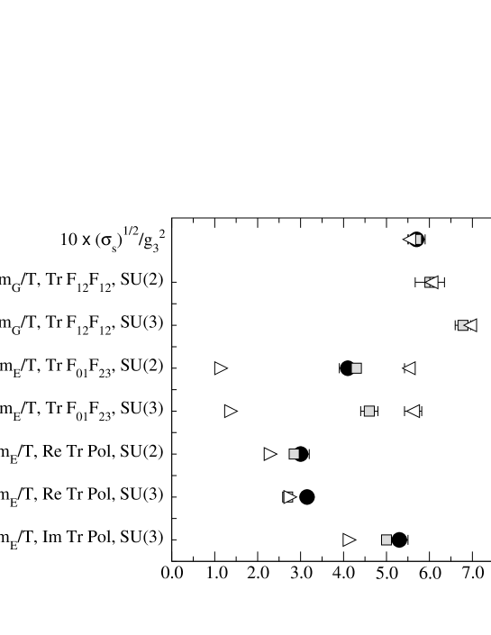
Figure 1: A comparison of spatial string tensions, as well as inverses of correlation lengths in various channels and two gauge groups, at $T\approx 2T_{c}^{\mbox{\scriptsize QCD}}$, with different methods, as explained in the text. The lattice data have been collected from Refs. [13, 19, 20, 21, 22]. Representative continuum operators have also been shown.

5.2 Pressure

We finally turn to the pressure. Unfortunately the situation remains somewhat open here. Not only has the non-perturbative $g^{6}$ term in Eq. (8) not been resolved, but we also do not have a “full 3d” prediction available: measurements can be carried out but a constant again remains open [24, 25]. These problems are ultimately due to the fact that the constant parts related to the divergent 4-loop matching coefficients in Eqs. (12), (14) have not been determined yet. The only unambiguous results are from 4d lattice simulations (at least for $N_{f}=0$), and from perturbation theory at asymptotically high temperatures.

Therefore, the best we can do is to see whether a necessary condition for the validity of the conjecture is satisfied: is it possible to find some value representing the unknown 4-loop constant terms, such that it reproduces a whole function of the expected type? This exercise is carried out in Fig. 2 (taken from Ref. [17]), and we indeed find that one can reproduce, in principle, a reasonable curve with a value of the constant of order unity.

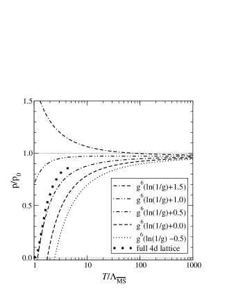
Figure 2: The pressure, normalised to the non-interacting Stefan-Boltzmann law $p_{0}$, for various values of the $\mathcal{O}(g^{6})$ constant term (from Ref. [17]; see there also for further details on what exactly is plotted here). The 4d lattice data is from Refs. [19, 23].

Of course, it must be said that due to the high perturbative order appearing, the pressure is an observable which is quite sensitive not only to the non-perturbative term but also to ambiguities in perturbation theory. For illustration, we demonstrate this in Fig. 3. An optimal value has been chosen for the constant, and then the renormalisation scale entering the expressions of the effective parameters in Eq. (2) has been varied within the range $0.5\bar{\mu}_{\mbox{\scriptsize opt}}...2.0\bar{\mu}_{\mbox{\scriptsize opt}}$, where $\bar{\mu}_{\mbox{\scriptsize opt}}\approx 6.7T$ is suggested by the next-to-leading order expression for $g_{\mbox{\scriptsize E}}^{2}$ [10].

The scale dependence is non-monotonic, because the first derivative of the result with respect to $\bar{\mu}$ is very close to vanishing, due to the fact that we have gone via the effective theory in Eq. (2) to obtain the output. Nevertheless, we see that at $T\mathop{\raise 1.29167pt\hbox{$<$\kern-7.5pt\raise-4.73611pt\hbox{$\sim$}}}3T_{c}^{\mbox{\scriptsize QCD}}$ ($T_{c}^{\mbox{\scriptsize QCD}}\sim\Lambda_{\overline{\rm MS}}$) the predictions are in any case getting unreliable, irrespective of the value of the constant. This may not be too surprising, though, since to determine the full $g^{6}$ constant term requires also renormalisation of $g$ at 2-loop level, but this has not been incorporated in the expressions shown here.

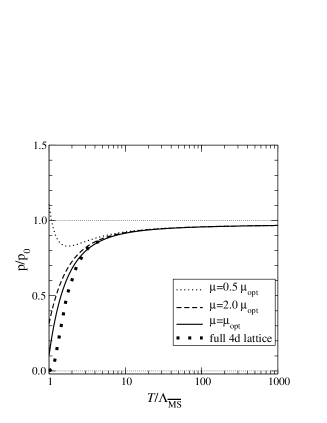
Figure 3: The dependence of the result of Fig. 2 on the renormalisation scale $\bar{\mu}$, around $\bar{\mu}_{\mbox{\scriptsize opt}}\approx 6.7T$, for an $\mathcal{O}(g^{6})$ constant $\sim 0.7$ (cf. Ref. [17]).

6 Conclusions

There is some numerical evidence for the conjecture of Sec. 3 from the spatial string tension as well as from various (“magnetic” and “electric”) correlation lengths, but more channels should be added. It would also be interesting to consider other observables (see, e.g., Ref. [26]).

The conjecture might also work for the pressure, although so far only one necessary condition is observed to be satisfied, and a lot of work remains to be carried out before we know whether a sufficient condition is there.

Once such analytic expressions with non-perturbative constants are known, extensions to finite $N_{f}>0$ and $\mu\mathop{\raise 1.29167pt\hbox{$<$\kern-7.5pt\raise-4.73611pt\hbox{$\sim$}}}\pi T$ are easy (see, e.g., Ref. [27]).

Hopefully similar expressions can be worked out also for real time observables, where 4d lattice simulations are even much more difficult.

References

- [1] J.O. Andersen, these proceedings [hep-ph/0210195]; A. Rebhan, these proceedings [hep-ph/0301130].
- [2] J.P. Blaizot, E. Iancu and A. Rebhan, Nucl. Phys. A698, 404 (2002) [hep-ph/0104033]; E. Braaten, Nucl. Phys. A702, 13 (2002); A. Peshier, Nucl. Phys. A702, 128 (2002) [hep-ph/0110342].
- [3] M.G. Alford, QCD at high density / temperature, hep-ph/0209287.
- [4] G. Cvetič and R. Kögerler, Phys. Rev. D66, 105009 (2002) [hep-ph/0207291].
- [5] A.D. Linde, Phys. Lett. B96, 289 (1980).
- [6] D.J. Gross, R.D. Pisarski and L.G. Yaffe, Rev. Mod. Phys. 53, 43 (1981).
- [7] P. Arnold and C. Zhai, Phys. Rev. D50, 7603 (1994) [hep-ph/9408276]; ibid. D51, 1906 (1995) [hep-ph/9410360].
- [8] C. Zhai and B. Kastening, Phys. Rev. D52, 7232 (1995) [hep-ph/9507380].
- [9] E. Braaten and A. Nieto, Phys. Rev. D53, 3421 (1996) [hep-ph/9510408].
- [10] K. Kajantie et al.,Nucl. Phys. B503, 357 (1997) [hep-ph/9704416].
- [11] P. Ginsparg, Nucl. Phys. B170, 388 (1980); T. Appelquist and R.D. Pisarski, Phys. Rev. D23, 2305 (1981).
- [12] E. Braaten and A. Nieto, Phys. Rev. Lett. 74, 3530 (1995) [hep-ph/9410218]; P. Arnold and L.G. Yaffe, Phys. Rev. D52, 7208 (1995) [hep-ph/9508280].
- [13] A. Hart and O. Philipsen, Nucl. Phys. B572, 243 (2000) [hep-lat/9908041]; A. Hart et al., Nucl. Phys. B586, 443 (2000) [hep-ph/0004060].
- [14] A. Dumitru and R.D. Pisarski, Phys. Rev. D66, 096003 (2002) [hep-ph/0204223].
- [15] O. Philipsen, these proceedings [hep-ph/0301128].
- [16] K. Kajantie, M. Laine and Y. Schröder, Phys. Rev. D65, 045008 (2002) [hep-ph/0109100]; Y. Schröder, hep-ph/0211288.
- [17] K. Kajantie et al., hep-ph/0211321.
- [18] Y. Schröder, in preparation; K. Kajantie et al., in preparation.
- [19] G. Boyd et al., Nucl. Phys. B469, 419 (1996) [hep-lat/9602007]; O. Kaczmarek et al., Phys. Rev. D62, 034021 (2000) [hep-lat/9908010].
- [20] M.J. Teper, Phys. Rev. D59, 014512 (1999) [hep-lat/9804008].
- [21] M. Laine and O. Philipsen, Nucl. Phys. B523, 267 (1998) [hep-lat/9711022]; Phys. Lett. B459, 259 (1999) [hep-lat/9905004].
- [22] S. Datta and S. Gupta, Phys. Lett. B471, 382 (2000) [hep-lat/9906023]; hep-lat/0208001.
- [23] A. Papa, Nucl. Phys. B478, 335 (1996) [hep-lat/9605004]; B. Beinlich et al., Eur. Phys. J. C6, 133 (1999) [hep-lat/9707023]; M. Okamoto et al. [CP-PACS Collaboration], Phys. Rev. D60, 094510 (1999) [hep-lat/9905005].
- [24] K. Kajantie et al., Phys. Rev. Lett. 86, 10 (2001) [hep-ph/0007109].
- [25] K. Kajantie et al., Nucl. Phys. B (Proc. Suppl.) 106, 525 (2002) [hep-lat/0110122]; hep-lat/0209072.
- [26] P. de Forcrand, M. D’Elia and M. Pepe, Phys. Rev. Lett. 86, 1438 (2001) [hep-lat/0007034]; P. Giovannangeli and C.P. Korthals Altes, Nucl. Phys. B608, 203 (2001) [hep-ph/0102022]; hep-ph/0212298.
- [27] A. Vuorinen, hep-ph/0212283.