Solution of coupled vertex and propagator Dyson-Schwinger equations in the scalar Munczek-Nemirovsky model

Abstract

In a scalar $\varphi^{2}\chi$ model, we exactly solve the vertex and $\varphi$ propagator Dyson-Schwinger equations under the assumption of a spatially constant (Munczek-Nemirovsky) propagator for the $\chi$ field. Various truncation schemes are also considered.

I Introduction

The Dyson-Schwinger equations (DSEs) DSE are an infinite system of coupled integral equations for the Green functions of a quantum field theory. In principle, their solution contains all possible information in the theory. However, the DSE for an $n$-point Green function involves various other Green functions of order $m\leq n+2$. So to make progress, the system must be truncated at some stage and models must be made for the unknown Green functions. For example, in QCD, the DSE for the quark propagator involves not only the quark propagator, but also the gluon propagator and the full quark-gluon vertex, both of which need to be calculated or modelled in some way for the equation to provide a solution for the quark propagator.

Notwithstanding the need for model input, the DSEs provide a relativistically covariant, non-perturbative approach to field theory that has enjoyed considerable success in recent years. In QCD, models based on the DSEs are able to describe accurately many facets of meson and, more recently, baryon physics in free space and at nonzero temperature and density Roberts:dr ; Roberts:2000aa . Additionally, recent DSE studies are now providing insight into the infrared behaviour of QCD Green functions and the nature of confinement IRreview ; gluonghost . Sophisticated studies have also been made of the DSEs in QED and other theories Roberts:dr ; Kizilersu:2000qd .

Almost all DSE based studies to date focus on the equations for some of the two point functions of the theory, making various models for the remaining two- and three-point functions. In this paper, we examine a simple theory and solve a larger system of equations. We consider a $\varphi^{2}\chi$ scalar field theory with a Munczek-Nemirovsky (MN) model propagator for the $\chi$ particle (which we introduce in Sec. II) and solve the coupled DSEs for the $\varphi$ propagator and 3-point vertex. An exact solution is possible in this model because relations amongst the Green functions allow the remaining system of DSEs to close without truncation. We also investigate the effect that imposing various truncations has on the solutions.

The central result of this analysis is that there is no real solution to the untruncated model unless the coupling is imaginary despite the model having solutions for real couplings when additional truncations of the DSEs are made. This is shown by the divergence of the diagrammatic expansion of the vertex.

The rest of this paper is structured in the following manner. We introduce the details of the model in Sec. II, and the various truncations we employ in Sec. III. In Sec. IV we show that the DSEs of the Munczek-Nemirovsky model close and derive their exact solution where it exists. Finally, we present our conclusions in Sec. V.

II Scalar model

We consider the theory of two scalar fields, $\varphi$ and $\chi$, described by the interaction Lagrangian:

$${\cal L}_{\rm int}=g\ \varphi^{2}\chi\,,$$ (1)

and work in Euclidean space. This scalar theory is primarily studied as a precursor for an investigation in QCD, but is also interesting in its own right and is sometimes used as a simplified description of meson-nucleon interactions. We define the momentum- (and position-) space propagators for the fields $\varphi$ and $\chi$ as $S(p)$ ($S(x,y)$) and $D(p)$ ($D(x,y)$) respectively. These objects satisfy the Dyson-Schwinger equations:

$$S^{-1}(p)=S_{0}^{-1}(p)+\Sigma(p)$$ (2)

and

$$D^{-1}(p)=D^{-1}_{0}(p)+\Pi(p)\,,$$ (3)

where the bare propagators are $S_{0}^{-1}(p)=(p^{2}+m^{2})$ for the $\varphi$ field of mass $m$ and $D_{0}^{-1}=(p^{2}+M^{2})$ for the $\chi$ field (mass $M$). The respective self-energies are defined as

$$\Sigma(p)=\int_{q}g\ D(q)S(p-q)\tilde{\Gamma}(p-q,p)$$ (4)

and

$$\Pi(p)=\frac{1}{2}\int_{q}g\ S(q)S(p+q)\tilde{\Gamma}(q,p+q)\,,$$ (5)

where $\tilde{\Gamma}(p,k)$ is the proper three-point vertex. (Here and in what follows momentum integrals are abbreviated as $\int_{q}=\int\frac{d^{4}q}{(2\pi)^{4}}$.) These equations are shown diagrammatically in Fig. 1. An additional (constant) tadpole contribution to Eq. (4) is omitted as it can be absorbed into the definition of the renormalised mass, $m$ Kuster:1996kx . Field renormalisation constants are suppressed as the ultraviolet divergences of the theory will be eliminated by the specific form of the $\chi$ propagator that we introduce below.

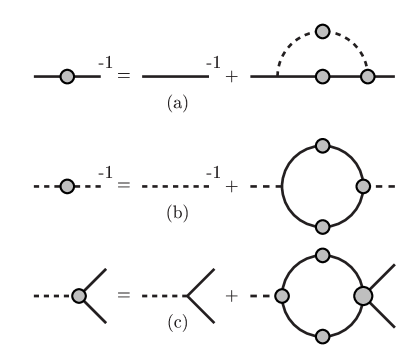
Figure 1: The Dyson-Schwinger equations for the (a) $\varphi$ and (b) $\chi$ propagators and (c) vertex function of the scalar theory of Eq. (1). Solid (dashed) lines are $\varphi$ ($\chi$) propagators and grey circles denote full one particle irreducible components.

The dependence of these equations on the vertex function $\tilde{\Gamma}$ means that they do not form a closed, computable system. An often used approach is to truncate the system at this level by introducing a model for $\tilde{\Gamma}$ and solve the resulting equations Ahlig:1998qf ; Tjon ; Sauli:2002qa . We investigate various possible truncations in Sec. III.

However, the vertex function satisfies its own DS equation [an inhomogeneous Bethe-Salpeter equation—see Fig. 1(c)] in terms of the propagators and an additional unknown function, the four-$\varphi$ scattering kernel, $K$:

$$\Gamma(p,k) \equiv g^{-1}\tilde{\Gamma}(p,k)$$

$$=\ 1+\int_{q}K(p,k,q)S(p+q)\Gamma(p+q,k+q)S(k+q)\,.$$

Here we have rescaled $\tilde{\Gamma}\to\Gamma$ to absorb the bare coupling of the theory. The scattering kernel, $K$, occurring in this equation is two particle irreducible with respect to the $\varphi$ legs and contains no annihilation contributions Roberts:dr . The same kernel also enters in investigations of two-body bound states in the Bethe-Salpeter approach Salpeter:sz . By keeping Eq. (II), it is possible to truncate the system at a higher level, modelling $K$ rather than $\Gamma$. This automatically ensures that the Dyson-Schwinger and bound state equations are truncated consistently.

In this paper, we will assume that the propagator for the $\chi$ field is constant throughout space-time. In momentum space this results in

$$g^{2}D(p)\equiv(2\pi)^{4}\alpha\ \delta^{4}(p)\,,$$ (7)

where $\alpha$ is the (constant) strength of the correlation. This is analogous to the approximation of Munczek and Nemirovsky (MN) Munczek:1983dx which has often been applied to model QCD MNpapers ; Bender:1996bb ; Bender:2002as . It was originally motivated as a simple means with which to provide the necessary infrared enhancement in the kernel of the quark DSE of QCD. However its physical foundations are fairly tenuous as it does not allow momentum transfer between quarks or their consequent scattering. Whilst it has this and other difficulties thesis , it also has the distinct advantage that the various integral equations of the DS system reduce to algebraic equations and it remains an interesting model.

With this scalar MN model in place, we will explore varying possible truncations in the following section and then show that they are unnecessary by solving the full set of equations and calculating the exact solutions (where they exist) in Sec. IV.

III Truncation schemes

In this section, we shall consider a number of truncations that can be applied to solve the DSEs above, each of which successively improves on the last. For simplicity, we omit the momentum dependence of propagators and vertices in what follows since the MN model decouples all differing momenta. In fact, the momentum only enters into the propagator and vertex DSEs though the bare propagator, $S_{0}^{-1}=p^{2}+m^{2}\equiv x$, so $\Gamma$, $\Sigma$, $S$ and $K$ depend only on $x$.

It is possible to define the dimensionless quantities $S^{\prime}=\sqrt{|\alpha|}S$, $\Sigma^{\prime}=\sqrt{|\alpha|}\Sigma$, $\Gamma^{\prime}=\Gamma$, $x^{\prime}=x/\sqrt{|\alpha|}$ and $K^{\prime}=K/|\alpha|$. If one works in terms of these new objects, all dependence on the magnitude of $\alpha$ will factorise in our analysis. Consequently, only the sign of this parameter is important. In order to avoid a proliferation of factors of $\alpha/|\alpha|$, we shall use the original (unprimed) quantities and only consider $\alpha=\pm 1$.

III.1 Rainbow truncation

For this scalar theory, the rainbow truncation is defined by

$$\Gamma_{\rm rainbow}(p,k)=1\,.$$ (8)

In QCD, when the analogous truncation of the quark DSE is combined with the ladder truncation of mesonic Bethe-Salpeter equations, the resulting models successfully describe the pseudo-scalar and light vector meson spectrum rainbowladder with additional higher-order corrections providing only minor modifications Bender:1996bb ; Bender:2002as . If the rainbow truncation is combined with the Munczek-Nemirovsky propagator, Eq. (7), the DSE for the $\varphi$ propagator reduces to a simple quadratic equation whose solutions are

$$S(x)=\frac{x\pm{\sqrt{x^{2}+4\,\alpha}}}{2\,\alpha}\,.$$ (9)

The physical solution and the corresponding self energy are shown as a function of $x=p^{2}+m^{2}$ as the dot-dashed curve in Fig. 2 for $\alpha=1$.

Figure 2: Dependence of the propagator (upper panel), self-energy (middle panel) and vertex function (lower panel) on the variable $x=p^{2}+m^{2}$ for $\alpha=1$. Solutions are shown for the bare- (dot-dashed), the one-loop- (short-dashed), two-loop- (long-dashed), two-loop-ladder- (dotted) vertices and for the ladder truncation of the vertex DS equation (solid).

III.2 One- and two-loop truncations

In the algebraic MN model, it becomes simple to include any finite order of contributions to the vertex. As no momentum flows along $\chi$ propagators and there are no complicating Dirac structures, every diagram at a given order contributes the same factor, For example, the one- and two- loop vertices are given by

$$\Gamma_{\rm 1\ loop}=1+\alpha\ S^{2},\quad\Gamma_{\rm 2\ loop}=1+\alpha\ S^{2}+4\alpha^{2}S^{4}\,,$$ (10)

respectively, where the factor of $4$ arises from diagram counting (see Sec. IV.1). These additional contributions to the vertex are not perturbative corrections; they involve the full propagator functions. Inserting these forms into the propagator DSE leads to 4th- and 6th- order equations for S whose physical solutions are also shown in Fig. 2 as the short- and long- dashed lines, respectively. The lower panels of the figure show the corresponding self energies and vertex functions. For comparison, we also show the solution (dotted line) when only the ladder dressings of the vertex are included to second order (that is, $\Gamma_{\rm 2\ loop}$ with a factor of 1 instead of 4) which we label as $\Gamma_{\rm 2\ loop}^{\prime}$.

III.3 Vertex ladder truncation

If (instead of explicitly approximating the vertex) we make a ladder truncation of the vertex kernel, $K(p,k,q)=g^{2}D(q)$, we are selecting an infinite class of planar diagrams (with non-perturbative propagators) to include in the vertex. At each order, we include the diagram that recursively dressed the contribution with one less loop Bender:2002as ; Delbourgo . However, even at the two loop level, contributions are already being omitted (compare $\Gamma_{\rm 2\ loop}$ and $\Gamma_{\rm 2\ loop}^{\prime}$).

With this truncation, Eq. (II) reduces to

$$\Gamma(p,k)=1+g^{2}\int_{q}D(q)S(p+q)\Gamma(p+q,k+q)S(k+q)\,.$$ (11)

Using the MN propagator, Eq. (7), gives the solution

$$\Gamma_{\rm ladder}=\sum_{i=0}^{\infty}\left(\alpha\ S^{2}\right)^{i}=\frac{1}{1-\alpha\ S^{2}}\,,$$ (12)

provided $\alpha\ S^{2}<1$. When this is inserted in the propagator DSE we arrive at a cubic equation for $S$:

$$S^{-1}=x+\frac{\alpha\ S}{1-\alpha\ S^{2}}\,.$$ (13)

The physical solution to this equation is given for $\alpha=1$ as the solid line in Fig. 2. The sum in Eq. (12) is seen to converge for all space-like and time-like $x$.

IV Coupled vertex and propagator equations

From comparison of the rainbow, one-loop, two-loop ladder ($\Gamma_{\rm 2\ loop}^{\prime}$), and full ladder solutions of the previous section (see Fig. 2), it is apparent that the approach to this ladder sum is monotonic and inclusion of such ladder diagrams beyond the first loop only results in small modifications Bender:2002as . However, further comparison with the full two-loop vertex solution (corresponding to $\Gamma_{\rm 2\ loop}$) indicates that the omitted diagrams may be important. In the simple MN model defined by Eq. (7), it is possible to go further and consistently include all contributions to the vertex. This is the main result of this article.

The generating functional of the theory we consider is

$${\cal Z}[J,j] = e^{{\cal W}[J,j]}$$

$$= \int{\cal D}\varphi{\cal D}\chi\exp\left[-\int{\cal L}-(\varphi,J)-(\chi,j)\right]\,,$$

where $J$($j$) is an external source for the $\varphi$($\chi$) field, ${\cal L}$ is the sum of the interaction Lagrangian, Eq. (1), and the usual kinetic pieces and the notation $(a,b)\equiv\int dx\,a(x)b(x)$. From this we can make a Legendre transform and define the effective action, ${\cal A}[\varphi,\chi]$ (with $\varphi=-\delta{\cal W}/\delta J$ and $\chi=-\delta{\cal W}/\delta j$), and thereby the one particle irreducible vertices,

$$\Gamma^{(n|m)}_{x_{1},\ldots,x_{n},y_{1},\ldots,y_{m}}=\frac{\delta^{n+m}{\cal A}[\varphi,\chi]}{\delta\varphi_{x_{1}}\ldots\delta\varphi_{x_{n}}\delta\chi_{y_{1}}\ldots\delta\chi_{y_{m}}}\,.$$ (15)

The DSEs arise from appropriate functional variation of this effective action. As usual, we can identify the position space propagators with the inverse two-point, one-particle irreducible (1-PI) vertices Itzykson:rh . For example,

$$S(x,y;J)=\frac{\delta^{2}{\cal W}}{\delta J_{x}\delta J_{y}}=\left(\frac{\delta^{2}{\cal A}}{\delta\varphi_{x}\delta\varphi_{y}}\right)^{-1}=\left(\Gamma^{(2|0)}_{xy}\right)^{-1}\,.$$ (16)

Thus,

$$K(w,x,y,z) = \Gamma^{(4|0)}_{wxyz}=\frac{\delta^{2}\Gamma^{(2|0)}_{yz}}{\delta\varphi_{w}\delta\varphi_{x}}$$ (17)

$$= \frac{\delta\Sigma(y,z;J)}{\delta S(w,x;J)}\,,$$

evaluated in the presence of external sources. For the last equality, we have used the position space analog of the DSE for the $\varphi$ propagator [Eq. (2)] to express $S^{-1}(x,y;J)$ in terms of $\Sigma(x,y;J)$, noting that $\delta S_{0}/\delta S$ vanishes.

By momentum conservation, the full 1-PI four-point scattering kernel, $K(p,q,r)$, is a function of three external momenta. However, in the MN reduction of the theory, no momentum is transferred through $\chi$ propagators and the scattering kernel describes two separate momentum flows. Consequently we only require $K(p,q,0)$. Further, since we only probe the $q=0$ limit of the vertex function in the vertex DSE, the $\varphi$ propagators in Eq. (II) must carry the same momentum and we only require $K(p,q=p,0)=\delta\Sigma(p)/\delta S(p)$.

Inserting the self energy from Eq. (4) and applying the derivative gives

$$K(p,p,0)=\frac{\delta\Sigma(p)}{\delta S(p)}=\int_{q}\left[\frac{\delta D(q)}{\delta S(p)}S(p-q)\Gamma(p-q,p)+D(q)\delta^{4}(p-q-p)\Gamma(p-q,p)+D(q)S(p-q)\frac{\delta\Gamma(p-q,p)}{\delta S(p)}\right]\,.$$ (18)

In principle, Eq. (3) determines the functional dependence of $D(q)$ on $S(p)$ through the polarisation loop in Eq. (5); pre- and post- multiplying both sides of Eq. (3) by factors of $D(q)$ and taking the derivative gives

$$-\frac{\delta D(q)}{\delta S(p)}=2D(q)S(q-p)\Gamma(q-p,p)D(q)+D(q)\int_{k}S(k)\frac{\delta\Gamma(k,k-q)}{\delta S(p)}S(q-k)D(p)\,.$$ (19)

However, the MN approximation, Eq. (7), presumably already invalidates Eq. (3) so this result may be misleading. As a simple alternative to Eq. (19), we also consider $\delta D(p)/\delta S(k)=0$.

We proceed by applying Eq. (7) to Eqs. (4), (II) and (18) to give

$$\Sigma=\alpha\ S\ \Gamma\,,\\$$ (20)

$$\Gamma=1+KS^{2}\Gamma\,,\\$$ (21)

$$K=\alpha\left[\Gamma+S\frac{\delta\Gamma}{\delta S}\right]+K_{D}\,.$$ (22)

If Eq. (19) is used to determine $\delta D/\delta S$, there is an additional contribution,

$$K_{D}=-\alpha^{2}S\ \Gamma\left[2S\ \Gamma+S^{2}\frac{\delta\Gamma}{\delta S}\right]\,,$$ (23)

to the kernel. For $\delta D/\delta S=0$, $K_{D}=0$. Momentum dependence is again suppressed in these equations as all quantities are at the same momentum. Combining the equations for the vertex and the kernel gives

$$\Gamma=1+\alpha\ S^{2}\Gamma\left(\Gamma\left[1-2\alpha\ S^{2}\Gamma\right]+S\frac{\delta\Gamma}{\delta S}\left[1-\alpha\ S^{2}\Gamma\right]\right)\,,$$ (24)

for $\delta D/\delta S$ determined from Eq. (19), and

$$\Gamma=1+\alpha\ S^{2}\Gamma^{2}+\alpha\ S^{3}\Gamma\frac{\delta\Gamma}{\delta S}\,,$$ (25)

for $\delta D/\delta S=0$. These functional differential equations are subject to the physical boundary condition that $\Gamma[0]=1$. This is simply the requirement that for an infinitely heavy $\varphi$ particle (whose propagator $S=1/m^{2}\stackrel{{\scriptstyle m\to\infty}}{{\longrightarrow}}0$), the vertex reduces to the bare vertex as loop corrections involving the $\varphi$ propagator vanish. Either of these equations, together with their boundary condition and Eqs. (2) and (20) close provided the functional derivative $\delta\Gamma/\delta S$ can be determined.

IV.1 Diagram counting

Physically, the use of the Munczek-Nemirovsky-like propagator, Eq. (7), means that $\chi$ field loops dressing the propagation of the $\varphi$ field or dressing the vertex carry no momentum. Consequently, objects such as the $\varphi$ self energy and the vertex can be expressed as appropriately weighted sums of products of dressed $\varphi$ propagators at the same momentum. That is, $\Gamma$ and $\Sigma$ are analytic functionals of $S$ and can be written as

$$\Gamma=\sum_{i=0}^{\infty}f_{i}(\alpha\ S^{2})^{i}\,,$$ (26)

and

$$\Sigma=\alpha\ S\sum_{i=0}^{\infty}e_{i}(\alpha\ S^{2})^{i}\,.$$ (27)

As a corollary, $\delta\Gamma/\delta S$ exists and can be defined. Indeed Eqs. (24) and (25) can both be rewritten as recursions amongst the coefficients $f_{i}$. For $\delta D/\delta S=0$, the relation is

$$f_{i}=\delta_{i0}+\sum_{j=0}^{i-1}(2j+1)f_{j}f_{i-j-1}\,.$$ (28)

These coefficients simply count the number of 1-PI contributions to the vertex dressing with $i$ loops in terms of full propagator lines. The first few coefficients are: 1, 1, 4, 27, 248, 2830, … and their asymptotic behaviour is $f_{n}\sim(2n+1)!!/e$ Stein from which it is apparent that the sum in Eq. (26) does not converge (nor is it Borel summable) for $\alpha\ S^{2}>0$. For the case of $\delta D/\delta S$ given by Eq. (19), an additional term

$$-2\sum_{j=0}^{i-2}\sum_{k=0}^{i-j-2}(k+1)f_{j}f_{k}f_{i-j-k-2}$$

appears on the right-hand side of Eq. (28) and the series is similarly divergent. The self energy coefficients, $e_{i}$, can also be calculated and a generating function can be constructed for them Arques .

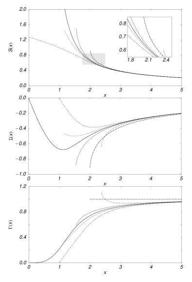
Figure 3: Dependence of the propagator (upper panel), self-energy (middle panel) and vertex function (lower panel) on the variable $x=p^{2}+m^{2}$ for $\alpha=-1$. Solutions are shown for the bare- (long-dashed), the one-loop- (dot-dashed), two-loop- (dot-dot-dashed) vertices, for the ladder truncation of the vertex DS equation (dotted), for the full solution with $\delta D/\delta S=0$ (short-dashed) and for the full solution with $\delta D/\delta S$ from Eq. (19) (solid). To clarify the various solutions for the propagator, the shaded region is expanded in the inset.

The apparent lack of solution is supported by the failure of various standard numerical methods NumRec to find a solution to either of the differential equations for $\Gamma$ with $\alpha>0$. This result is perhaps not unexpected since the theories defined by the Lagrangian of Eq. (1) and the related $\varphi^{3}$ theory are unstable as they have no ground state Dyson:tj ; Baym ; Tjon ; Schreiber ; Cornwall:1995dr . However, the effect that the use of the MN model for the $\chi$ propagator has on these conclusions is difficult to assess.

IV.2 Numerical solution for $\alpha<0$

If we consider $\alpha<0$ (as discussed at the beginning of Sec. III, the magnitude of $\alpha$ is unimportant), solutions of Eqs. (24 )and (25) exist. For this to be the case, the theory either has an imaginary coupling, $g=ih$ ($h\in R\!\!\!\!\!\!I\;$), or the correlation between the $\chi$ fields at two points is negative so the fields are imaginary valued. The first scenario corresponds to a non-Hermitian Hamiltonian that is ${\cal PT}$-symmetric. Such theories retain a positive energy spectrum and have been considered in detail by Bender et al. Bender .

The numerical solution of the vertex differential equations and their boundary condition is straightforward for $\alpha<0$ (the functional nature is irrelevant because of the decoupling of propagators at different momenta). Once we have determined the functional dependence of the vertex on $S$, we can combine that with Eqs. (2) and (20) and obtain exact solutions to the MN model.

Figure 3 depicts the momentum dependence of the $\varphi$ propagator, the self-energy and the vertex as a function of $x$ for $\alpha=-1$ and for the two alternate determinations of $\delta D/\delta S$. The solid line corresponds to $\delta D/\delta S$ determined from Eq. (19), while the short-dashed line is for $\delta D/\delta S=0$. For comparison, we also show the ($\alpha=-1$) solutions obtained using various of the truncations of the preceding section. For $\alpha<0$, most of the algebraic solutions become complex at some critical value of $x$, hence the abrupt termination of the solutions in the figure. Numerically we find that the full solution for $\delta D/\delta S=0$ has a critical point $x_{\rm crit}=1.518\sqrt{|\alpha|}$, although it is not known whether this critical behaviour has any physical significance. For $\delta D/\delta S$ determined from Eq. (19), the solution exists for all $x$. It is also evident from the figure that the various analytic solutions beyond the bare vertex provide a reasonable approximation to the full solution for moderate to large momenta as should be expected.

IV.3 Higher-point vertices

Figure 4: Behaviour of the higher point Green functions as functionals of $S$ and functions of $x$ as described in the text.

We now know the functional dependence of $\Gamma[S]$ ($=\Gamma^{(2|1)}$) and, through Eq. (18), of $K[S]$ ($=\Gamma^{(4|0)}$) for $\alpha<0$. Consequently, we can (numerically) construct every 1-PI Green function of the theory with zero or one external $\chi$ leg carrying zero momentum and any number of pairs of $\varphi$ legs carrying the same momentum. Figure 4 shows $\Gamma^{(2|0)}$ (short-dashed), $\Gamma^{(2|1)}$ (dotted), $\Gamma^{(4|0)}$ (long-dashed), $\Gamma^{(4|1)}$ (dot-dashed), $\Gamma^{(6|0)}$ (solid) as functionals of $S$ (upper panel) and as functions of $x$ (lower panel) given the numerical solution for $S$, all with $\alpha=-1$ and $\delta D/\delta S$ obtained from Eq. (19).

Since we do not know the behaviour of $K(p,q\neq p,0)$, we cannot apply the results of this analysis to the study of massive bound states within the model as was done in Ref. Bender:2002as for the ladder vertex truncation.

V Summary

The analysis in this paper demonstrates that the exact MN model defined by Eq. (7) has no solutions for positive values of the coupling $\alpha$. However when additional truncations are introduced for the vertex or for the scattering kernel, solutions can be found. (It is of course perfectly reasonable to define the MN model to include the bare vertex truncation.) For the case of $\alpha<0$ we solve the full MN model and investigate how well various truncations approximate the full solution.

The extension to a more QCD-like theory (which was the motivation for this study) through the use of fermion and vector boson fields appears possible after the complications introduced by the Dirac structure are addressed. This will result in coupled, partial differential equations for the propagator dependence of the various Dirac components of the fermion-gauge boson vertex. Since QCD and more realistic models of it do not suffer from the fundamental difficulties of the scalar theory considered here, the problems of solution existence that we encountered would likely not persist. As a further extension of this work, there may be some scope to extend this analysis to models with less restrictive $\chi$ propagators such as Gaussian forms gaussian .

- (1) F. J. Dyson, Phys. Rev. 75, 486 (1949); ibid 75, 1736 (1949). J. S. Schwinger, Proc. Nat. Acad. Sci. 37, 452 (1951); ibid 37, 455 (1951);
- (2) C. D. Roberts and A. G. Williams, Prog. Part. Nucl. Phys. 33, 477 (1994).
- (3) C. D. Roberts and S. M. Schmidt, Prog. Part. Nucl. Phys. 45, S1 (2000).
- (4) R. Alkofer and L. von Smekal, Phys. Rept. 353, 281 (2001).
- (5) C. S. Fischer and R. Alkofer, Phys. Lett. B 536, 177 (2002); P. Watson and R. Alkofer, Phys. Rev. Lett. 86, 5239 (2001); C. Lerche and L. von Smekal, Phys. Rev. D 65, 125006 (2002); J. C. R. Bloch, Phys. Rev. D 64, 116011 (2001); D. Zwanziger, arXiv:hep-th/0206053.
- (6) A. Kızılersü, A. W. Schreiber and A. G. Williams, Phys. Lett. B 499, 261 (2001).
- (7) J. Küster and G. Münster, Z. Phys. C 73, 551 (1997).
- (8) S. Ahlig and R. Alkofer, Annals Phys. 275, 113 (1999).
- (9) T. Nieuwenhuis and J. A. Tjon, Phys. Rev. Lett. 77, 814 (1996); F. Gross, C. Savkli and J. Tjon, Phys. Rev. D 64, 076008 (2001).
- (10) V. B. Sauli, arXiv:hep-ph/0211221.
- (11) E. E. Salpeter and H. A. Bethe, Phys. Rev. 84, 1232 (1951).
- (12) H. J. Munczek and A. M. Nemirovsky, Phys. Rev. D 28, 181 (1983).
- (13) A. C. Aguilar et al., Phys. Rev. D 62, 094014 (2000); A. Bender et al., Phys. Lett. B 516, 54 (2001); J. C. Bloch et al., Phys. Rev. C 60, 065208 (1999); C. Y. Cheung and W. M. Zhang, Phys. Rev. D 60, 014017 (1999); P. Maris et al., Phys. Rev. C 57, 2821 (1998); D. Blaschke et al., Phys. Lett. B 425, 232 (1998); D. W. McKay and H. J. Munczek, Phys. Rev. D 55, 2455 (1997); A. Bender et al., Phys. Rev. Lett. 77, 3724 (1996); C. J. Burden et al., Phys. Lett. B 285, 347 (1992); P. Jain and H. J. Munczek, Phys. Rev. D 44, 1873 (1991).
- (14) A. Bender, C. D. Roberts and L. von Smekal, Phys. Lett. B 380, 7 (1996).
- (15) A. Bender, W. Detmold, C. D. Roberts and A. W. Thomas, Phys. Rev. C 65, 065203 (2002).
- (16) W. Detmold, Nonperturbative approaches to Quantum Chromodynamics, Ph.D. thesis, University of Adelaide, 2002.
- (17) P. Maris and C. D. Roberts, Phys. Rev. C 56, 3369 (1997); P. Maris and P. C. Tandy, Phys. Rev. C 60, 055214 (1999)
- (18) R. Delbourgo, D. Elliott and D. S. McAnally, Phys. Rev. D 55, 5230 (1997); R. Delbourgo, A. C. Kalloniatis and G. Thompson, Phys. Rev. D 54, 5373 (1996).
- (19) C. Itzykson and J. B. Zuber, Quantum Field Theory,, (McGraw-Hill, 1980).
- (20) A. Pelster, H. Kleinert and M. Bachmann, Annals Phys. 297, 363 (2002).
- (21) A. Petermann, Arch. Sci. Soc. Phys. Hist. Nat. Genève 6, 5 (1953); Phys. Rev. 89, 1160 (1953).
- (22) P. Cvitanovic, B. Lautrup and R. B. Pearson, Phys. Rev. D 18, 1939 (1978).
- (23) P. R. Stein, J. Comb. Th. A 24,357 (1978); P. R. Stein and C. J. Everett, Disc. Math. 21, 309 (1978).
- (24) D. J. Broadhurst and D. Kreimer, Phys. Lett. B 475, 63 (2000); Nucl. Phys. B 600, 403 (2001).
- (25) D. Arquès and J.-F. Béraud, Disc. Math. 215, 1 (2000).
- (26) W. H. Press, S. A. Teukolsky, W. T. Vetterling and B. P. Flannery, Numerical Recipes in FORTRAN : the art of scientific computing, (Cambridge University Press,1992).
- (27) F. J. Dyson, Phys. Rev. 85, 631 (1952).
- (28) G. Baym, Phys. Rev. 117, 886 (1959).
- (29) R. Rosenfelder and A. W. Schreiber, Eur. Phys. J. C 25, 139 (2002); Phys. Rev. D 53, 3337 (1996); Phys. Rev. D 53, 3354 (1996).
- (30) J. M. Cornwall and D. A. Morris, Phys. Rev. D 52, 6074 (1995).
- (31) C. M. Bender, K. A. Milton and V. M. Savage, Phys. Rev. D 62, 085001 (2000); C. M. Bender, S. Boettcher, P. N. Meisinger and Q. h. Wang, Phys. Lett. A 302, 286 (2002).
- (32) C. J. Burden, L. Qian, C. D. Roberts, P. C. Tandy and M. J. Thomson, Phys. Rev. C 55, 2649 (1997); A. C. Aguilar, A. A. Natale and R. Rosenfeld, Phys. Rev. D 62, 094014 (2000).