The $\eta$ $\to$ $\pi^{0}\pi^{0}\gamma\gamma$ decay in Generalized chiral perturbation theory

Abstract

Calculations of $\eta$ $\to$ $\pi^{0}\pi^{0}\gamma\gamma$ decay in Generalized chiral perturbation theory are presented. Tree level and some of next-to-leading corrections are involved. Sensitivity to violation of the Standard counting is discussed.

1 Introduction

The $\eta(p\,)\to\pi^{0}(p_{1})\,\pi^{0}(p_{2})\,\gamma(k)\,\gamma(k^{\prime})$ process is a rare decay, which has been recently studied by several authors in context of Standard chiral perturbation theory (S$\chi$PT), namely at the lowest order by Knöchlein, Scherer and Drechsel [1] and to next-to-leading by Bellucci and Isidori [2] and Ametller et al.[3]. The experimental interest for such a process comes from the anticipation of large number of $\eta$’s to be produced at various facilities. The goal of our computations is to add the result for the next-to-leading order in Generalized chiral perturbation theory (G$\chi$PT). The motivation is that one of the important contributions involve the $\eta\,\pi\to\eta\,\pi$ off-shell vertex which is very sensitive to the violation of the Standard scheme and thus this decay provides a possibility of its eventual observation. We have completed the calculations at the tree level, added 1PI one loop corrections and phenomenological corrections of the resonant contribution. These preliminary results we would like to present in this paper.

2 Kinematics and parameters

The amplitude of the process can be defined

$$\langle\pi^{0}(p_{1})\pi^{0}(p_{2})\gamma(k,\epsilon)\gamma(k^{{}^{\prime}},\epsilon^{{}^{\prime}})_{out}|\eta(p)_{in}\rangle=i(2\pi)^{4}\delta^{(4)}(P_{f}-p){\cal M}_{fi}.$$ (1)

In the square of the amplitude summed over the polarizations

$$\overline{|{\cal M}_{fi}|^{2}}=\sum_{pol.}|{\cal M}_{fi}|^{2},$$ (2)

only three independent Lorentz invariant variables occur

$$s_{\gamma\gamma}=(\>k+k^{\prime})^{2},\quad s_{\pi\pi}=(p_{1}+p_{2})^{2},\quad k.P_{\pi\pi}=k.(p_{1}+p_{2}),$$ (3)

where $s_{\gamma\gamma}$ resp. $s_{\pi\pi}$ can be interpreted as diphoton resp. dipion energy squares. $k.P_{\pi\pi}$ can be expressed in terms of $s_{\pi\pi},s_{\gamma\gamma}$ and the angle $\vartheta_{\gamma}$ between the direction of the diphoton and one of the photons in the center of mass of the diphoton. The range of the kinematic variables is

$$0<\,s_{\gamma\gamma}\leq\,(M_{\eta}-2M_{\pi})^{2},\quad 4M_{\pi}^{2}\leq\,s_{\pi\pi}\leq\,(M_{\eta}-\sqrt{s_{\gamma\gamma}})^{2},\quad-1\leq\,\cos\vartheta_{\gamma}\leq 1\,.$$ (4)

Our goal is to calculate the partial decay width of the $\eta$ particle as the function of the diphoton energy square $s_{\gamma\gamma}$

$$\frac{\textrm{d}\Gamma}{\textrm{d}s_{\gamma\gamma}}\ =\ \frac{1}{(8\pi)^{5}M_{\eta}^{3}}\,\int\overline{\rule{0.0pt}{11.38092pt}|{\mathcal{M}}_{fi}|^{2}}\,\lambda^{1/2}(M_{\eta}^{2},s_{\gamma\gamma},s_{\pi\pi})\sqrt{1-\frac{4M_{\pi}^{2}}{s_{\pi\pi}}}\;\textrm{d}\cos\vartheta_{\gamma}\,\textrm{d}s_{\pi\pi}.$$ (5)

At the lowest order, the S$\chi$PT does not depend on any unknown free order parameters. In contrast, there are two free parameters controlling the violation of the Standard picture in the Generalized scheme. We have chosen them as

$$r\ =\ \frac{m_{s}}{\hat{m}}\,,\quad X_{GOR}\ =\ \frac{2B\hat{m}}{M_{\pi}^{2}}$$ (6)

and their ranges are $r\sim r_{1}-r_{2}\sim 6-26\,,\ 0\ \leq\ X_{GOR}\ \leq\ 1$. The Standard values of these parameters are $r=r_{2}$ and $X_{GOR}=1$. In the Standard counting also $\Delta_{GMO}=0$, where

$$\Delta_{GMO}=\frac{3M_{\eta}^{2}+M_{\pi}^{2}-4M_{K}^{2}}{M_{\pi}^{2}}.$$ (7)

We use abbreviations for

$$\hat{m}\ =\ \frac{m_{u}+m_{d}}{2}\,,\ R\ =\ \frac{m_{s}-\hat{m}}{m_{d}-m_{u}}$$ (8)

$$r_{1}=2\,\frac{M_{K}}{M_{\pi}}-1,\ \,r_{2}=2\,\frac{M_{K}^{2}}{M_{\pi}^{2}}-1$$ (9)

and

$$\varepsilon=2\,\frac{r_{2}-r}{r^{2}-1}\;.$$ (10)

3 Tree level

At the $O(p^{4})$ tree level, the amplitude has two contributions, with a pion and an eta propagator. The first one is resonant and thus we call it ‘$\pi^{0}$-pole’, the other is nonresonant ‘$\eta$-tail’. The amplitude of the $\pi^{0}$-pole contribution is

$$i{\mathcal{M}}_{fi}^{(R)}\ =\ -\,\frac{3ie^{2}\Delta_{\pi\eta}\alpha_{R}}{16\sqrt{3}\pi^{2}F_{\pi}^{3}R}\;\varepsilon^{\alpha\beta\mu\nu}\;\varepsilon^{*}_{\alpha}(\,k,\lambda)\,\varepsilon^{*}_{\beta}(\,k^{\prime},\lambda^{\prime})\;k_{\mu}k^{\prime}_{\nu}\;\frac{1}{s_{\gamma\gamma}-M_{\pi}^{2}}\;,$$ (11)

where $\ \Delta_{\pi\eta}=M_{\eta}^{2}-M_{\pi}^{2}\$,

$$\alpha_{R}\ =\ \frac{4\,\delta}{\sqrt{3}}\ +\ \frac{2M_{\pi}^{2}(r-1)}{\Delta_{\pi\eta}}\;\bigg{[}\;\frac{1}{3}\;(\alpha_{\pi\pi}-1)\;\Big{(}1-\frac{4\,\delta}{\sqrt{3}}\;\Big{)}\ +\ \frac{\Delta_{GMO}}{(r-1)^{2}}\;\Big{(}1+\frac{4\,\delta}{\sqrt{3}}\;\Big{)}\,\bigg{]}.$$ (12)

and $\ \alpha_{\pi\pi}\;=\;1+(6(1-X_{GOR})+3r\varepsilon)/(r+2)\ .$ In the Standard limit $\ \alpha_{R},\alpha_{\pi\pi}=1$. $\ \delta/R\$ is the $\eta-\pi^{0}$ mixing angle

$$\delta\ =\ \frac{\sqrt{3}}{4}\;\Big{[}\,1+\frac{M_{\pi}^{2}}{3\Delta_{\eta\pi}}\;\big{(}(r-1)^{2}\,\varepsilon-3\Delta_{GMO}\big{)}\Big{]}.$$ (13)

The structure of the $\eta$-tail amplitude is similar

$$i{\mathcal{M}}_{fi}^{(\eta)}\ =\ \frac{ie^{2}M_{\pi}^{2}\,\alpha_{\pi\eta}}{12\sqrt{3}\pi^{2}F_{\pi}^{3}}\;\varepsilon^{\alpha\beta\mu\nu}\;\varepsilon^{*}_{\alpha}(\,k,\lambda)\,\varepsilon^{*}_{\beta}(\,k^{\prime},\lambda^{\prime})\;k_{\mu}k^{\prime}_{\nu}\;\frac{1}{s_{\gamma\gamma}-M_{\eta}^{2}}\;.$$ (14)

The constant $\alpha_{\pi\eta}$ is

$$\alpha_{\pi\eta}\ =\ 1\ +\ \frac{(1+2r)(2(1-X_{GOR})+r\,\varepsilon)}{2+r}\ -\ \frac{2{\Delta}_{GMO}}{r-1}\;.$$ (15)

The Standard values of the contributions to the partial decay rate and the maximum possible violation of the Standard counting ($r=r_{1},X_{GOR}=0$) are represented in fig.1. The pole of the resonant contribution at $s_{\gamma\gamma}=M_{\pi}^{2}\,\sim\,0.06M_{\eta}^{2}$ is transparent. While in the Standard case it is fully dominant, in the Generalized scheme the $\eta$-tail could be determining in the whole area $s_{\gamma\gamma}>0.11M_{\eta}^{2}$. The reason can be found in the constant $\alpha_{\pi\eta}$ from the $\eta\,\pi\to\eta\,\pi$ vertex. Its Standard value is equal to $\alpha_{\pi\eta}=1$, but in the Generalized counting it could jump up to $\alpha_{\pi\eta}\sim 16$. Compared to $\alpha_{\pi\eta}$, $\alpha_{R}$ is not so sensitive, maximum value is $\alpha_{R}\sim 1.5$ for $r=15,X_{GOR}=1$.

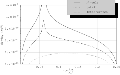
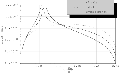
Figure 1: S$\chi$PT and G$\chi$PT contributions to the partial decay rate $\textrm{d}\Gamma/\textrm{d}z_{\gamma}$

The full decay width for the Standard ($r=r_{2},X_{GOR}=1,\Delta_{GMO}=0$) and Generalized case ($r=r_{2}$,$X_{GOR}=0.5$ and $r=r_{1}$,$X_{GOR}=0$) is displayed in fig.2. It can be seen, that even in the conservative intermediate case the change is quite interesting.

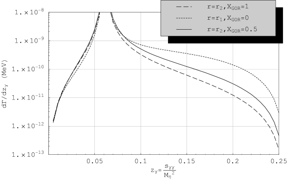
Figure 2: Full tree level decay width depending on the parameters $r$ and $X_{GOR}$

4 One loop corrections

There are four distinct contributions at the next-to-leading order: one loop corrections to the $\pi^{o}$-pole and the $\eta$-tail, one particle irreducible diagrams and counterterms. In the latter case we will rely upon the results of [3]. Their estimate from vector meson dominated counterterms indicates, that it causes only a slight decrease of the full decay width. Because the estimate is the same for both schemes, for our purpose of studying the differences between them we can leave it for later investigation.

More important might be the corrections to the $\eta$-tail diagram. At the present time, although we do have the amplitude, we are still working at the numerical analysis. We decided, similarly to [2], to correct the $\pi^{0}$-pole amplitude (11) by a phenomenological parametrization of the $\eta\to 3\pi^{0}$ vertex and fix the parameters from experimental $\eta\to 3\pi^{0}$ data:

$$iA_{corr}(\eta\to 3\pi^{0})\ =\ -\;\frac{3i\Delta_{\pi\eta}}{4\sqrt{3}F_{\pi}^{2}R}\,\varrho\,e^{i\phi_{R}}i{\mathcal{M}}_{fi}^{(R)}\;\;\;\;\;\;\;\;\;\;\;\;\;\;\;\;\;\;\;\;\;\;\;\;\;\;\;\;\;\;\;\;\;\;\;\;$$ (16)

$$\ =\ -\,\frac{3ie^{2}\Delta_{\pi\eta}}{16\sqrt{3}\pi^{2}F_{\pi}^{3}R}\;\varrho\,e^{i\phi_{R}}\;\varepsilon^{\alpha\beta\mu\nu}\;\varepsilon^{*}_{\alpha}(\,k,\lambda)\,\varepsilon^{*}_{\beta}(\,k^{\prime},\lambda^{\prime})\;k_{\mu}k^{\prime}_{\nu}\;\frac{1}{s_{\gamma\gamma}-M_{\pi}^{2}}\;.$$ (17)

The factor $\varrho$ can be fixed from the experimental results for $\eta\to 3\pi^{0}$ [2]

$$-\,\frac{3\Delta_{\pi\eta}}{4R}\ =\ M_{K^{\pm}}^{2}-M_{K^{0}}^{2}+M_{\pi^{0}}^{2}-M_{\pi^{\pm}}^{2},\quad\varrho\ =\ 2.0\ \pm\ 0.1\,.$$ (18)

As the phase $\phi_{R}$ cancels in the square of the amplitude, it cannot be determined that way. It is possible to make an estimate by expanding the $\eta\to 3\pi^{0}$ one loop amplitude around the center of the Dalitz Plot [2]. By performing this procedure in the Generalized scheme it can be found

$$\phi_{R}\ =\ \frac{1}{96\pi F_{\pi}^{2}}\,\sqrt{1-\frac{12M_{\pi}^{2}}{M_{\eta}^{2}-3M_{\pi}^{2}}}\ \Big{[}\,2M_{\eta}^{2}+M_{\pi}^{2}\,\big{(}11\,\alpha_{\pi\pi}-2\big{)}\Big{]}.$$ (19)

The 1PI amplitude, where we neglected the suppressed kaon loops, can be expressed as

$$i{\mathcal{M}}_{fi}^{(1PI)}\ =\ \frac{e^{2}}{12\sqrt{3}\pi^{2}F_{\pi}^{5}}\;\varepsilon^{\alpha\beta\mu\nu}\;\varepsilon^{*}_{\alpha}(\,k,\lambda)\,\varepsilon^{*}_{\varrho}(\,k^{\prime},\lambda^{\prime})\;k_{\beta}p_{\nu}\,[\,k^{\prime}_{\mu}q^{\varrho}-\delta_{\mu}^{\varrho}\;q.k^{\prime}\,]$$

$$\times\ [\,3s_{\pi\pi}+M_{\pi}^{2}(\,\alpha_{\pi\pi}-4\,)]\;F(\,k^{\prime},\,q\,)\ +\ (\,k\leftrightarrow k^{\prime}),$$ (20)

where $\,q=p-k\$ and

$$F(\,k^{\prime},\,q\,)\Big{|}_{{k^{\prime}}^{2}=0}=\frac{1}{2(q.k^{\prime})^{2}}\,\bigg{[}\Big{(}\,\frac{i}{8\pi^{2}}-4M_{\pi}^{2}\,C_{0}(k^{\prime},\,q)\Big{)}\,q.k^{\prime}+\Big{(}\,B_{0}(k^{\prime},\,q)-B_{0}(q)\Big{)}\,q^{2}\bigg{]}.$$ (21)

$C_{0}(\,x,y\,)$ and $B_{0}(x)$ are the standard scalar two and three point functions [5]. In the square of the amplitude we can distinguish the following contributions

$$\overline{\rule{0.0pt}{11.38092pt}|{\mathcal{M}}_{fi}|^{2}}\ =\ \sum_{pol.}\,\Big{[}\ |{\mathcal{M}}^{(R)}_{fi}|^{2}+|{\mathcal{M}}^{(1PI)}_{fi}|^{2}+{\mathcal{M}}_{fi}^{(1PI-R)}+{\mathcal{M}}_{fi}^{(\eta)\;2}\,\Big{]}\,,$$ (22)

where ${\mathcal{M}}_{fi}^{(1PI-R)}$ is the 1PI-resonant interference and

$${\mathcal{M}}_{fi}^{(\eta)\;2}\ =\ |{\mathcal{M}}^{(\eta)}_{fi}|^{2}+{\mathcal{M}}_{fi}^{(1PI-\eta)}+{\mathcal{M}}_{fi}^{(R-\eta)}$$ (23)

is the effect of the $\eta$-tail diagram. ${\mathcal{M}}_{fi}^{(1PI-\eta)}$ and ${\mathcal{M}}_{fi}^{(R-\eta)}$ are the interference terms denoted in the same way as ${\mathcal{M}}_{fi}^{(1PI-R)}$.

Similarly to the tree level case, fig.3 represents the relevant contributions to the decay width for the Standard and the maximum violation of the Standard scheme. The absolute value of the interference terms is drawn.

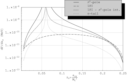
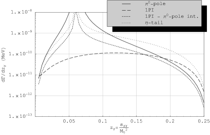
Figure 3: S$\chi$PT and G$\chi$PT contributions to the partial decay rate $\textrm{d}\Gamma/\textrm{d}z_{\gamma}$

Indeed, at the left picture we reproduce the results of [1], [2] and [3]. The 1PI–resonant interference is destructive for $s_{\gamma\gamma}>M_{\pi}^{2}$ and constructive otherwise. This confirms the results of Ametller et al.[3] and is in contradiction to work of Bellucci and Isidori [2]. Moving to the Generalized counting, the 1PI graphs does not dramatically influence the indications of the tree level. Fig.4 displays the corrected decay width in both extremes of the parameters. For comparison, also the change in 1PI diagrams is shown.

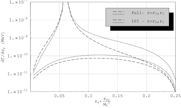
Figure 4: One loop corrected full decay width and the 1PI graphs’ contribution

5 Conclusion

We have analyzed the $\eta\to\pi^{0}\pi^{0}\gamma\gamma$ decay to the next-to-leading order of chiral perturbation theory in its both variants. There are four distinct contributions – the $\pi^{0}$-pole, $\eta$-tail, 1PI and counterterms.

The calculation in the Standard limit of the theory proved the dominance of the resonant pion pole contribution in the kinematic region $s_{\gamma\gamma}<0.20M_{\eta}^{2}$. The $\eta$-tail graph is small in the whole phase space. The 1PI diagrams can’t be omitted, they are dominant for $s_{\gamma\gamma}>0.20M_{\eta}^{2}$. Our calculations confirm the destructive 1PI-resonant interference in the area $s_{\gamma\gamma}>M_{\pi}^{2}$.

The Generalized counting brought some important changes. The 1PI contribution could grow around 50%, the $\eta$-tail up to 50 times. The latter one could become dominant in the whole region $s_{\gamma\gamma}>0.11M_{\eta}^{2}$.

In the full partial decay width, the possible violation of the Standard scheme is considerable. Relying upon the work [3], we neglected the counterterm contribution. We left open the questions about the higher order corrections to the $\eta$-tail amplitude and the experimental value of our calculations.
Acknowledgments: This work was supported by program ‘Research Centers’ (project number LN00A006) of the Ministry of Education of Czech Republic.

References

- [1] G. Knöchlein, S. Scherer, D. Drechsel, Phys. Rev. D53 (1996) 3634-3642
- [2] S. Bellucci, G. Isidori, Phys. Lett. B405 (1997) 334-340
- [3] Ll. Ametller, J. Bijnens, A. Bramon, P. Talavera, Phys. Lett. B400 (1997)370-378
- [4] S. Bellucci: to 1-Loop in ChPT, presented at the ‘Workshop on Hadron Production Cross Sections’ at DAPHNE, Karlsruhe, Nov.1-2, 1996, hep-ph/9611276
- [5] M. Veltman: Diagrammatica, Cambridge University Press, 1994