Thermalization of fermionic
quantum fields

We solve the nonequilibrium dynamics of a $3+1$ dimensional theory with Dirac fermions coupled to scalars via a chirally invariant Yukawa interaction. The results are obtained from a systematic coupling expansion of the 2PI effective action to lowest non-trivial order, which includes scattering as well as memory and off-shell effects. The dynamics is solved numerically without further approximation, for different far-from-equilibrium initial conditions. The late-time behavior is demonstrated to be insensitive to the details of the initial conditions and to be uniquely determined by the initial energy density. Moreover, we show that at late time the system is very well characterized by a thermal ensemble. In particular, we are able to observe the emergence of Fermi–Dirac and Bose–Einstein distributions from the nonequilibrium dynamics.

1 Introduction

The abundance of experimental data on matter in extreme conditions from relativistic heavy-ion collision experiments, as well as applications in astrophysics and cosmology has lead to a strong increase of interest in the dynamics of quantum fields out of equilibrium. Experimental indications of thermalization in collision experiments and the justification of current predictions based on equilibrium thermodynamics, local equilibrium or (non–)linear response pose major open questions for our theoretical understanding [1, 2]. One way to resolve these questions is to try to understand quantitatively the far-from-equilibrium dynamics of quantum fields, without relying on the assumption of small departures from equilibrium, or on a possible separation of scales that forms the basis of effective kinetic descriptions [3]. In contrast to close-to-equilibrium approaches, the quantum-statistical fluctuations of the fields are not assumed to be described by a thermal ensemble. Moreover, one goes beyond the range of applicability of the usual gradient expansion and dilute-gas approximation.

In contrast to thermal equilibrium, which keeps no information about the past, nonequilibrium dynamics poses an initial value problem: time-translation invariance is explicitly broken by the presence of the initial time, where the system has been prepared. The question of thermalization investigates how the system effectively looses the dependence on the details of the initial condition, and becomes approximately time-translation invariant at late times. According to basic principles of equilibrium thermodynamics, the thermal solution is universal in the sense that it is independent of the details of the initial condition and is uniquely determined by the values of the (conserved) energy density and of possible conserved charges. There are two distinct classes of universal behavior, corresponding to Bose-Einstein and Fermi-Dirac statistics respectively.

The description of the effective loss of initial conditions and subsequent approach to thermal equilibrium in quantum field theory requires calculations beyond so–called “Gaussian” (leading-order large–$N$, Hartree or mean-field type) approximations [4, 5, 6]. Similar to the free-field theory limit, these approximations typically exhibit an infinite number of additional conserved quantities which are not present in the underlying interacting theory [7, 8]. These spurious constants of motion constrain the time evolution and lead to a non-universal late-time behavior [9]. It has recently been demonstrated in the context of scalar field theories, that the approach to quantum thermal equilibrium can be described by going beyond these approximations [10, 9]. In particular, this has been achieved by using a systematic coupling expansion [10] or a $1/N$ expansion to next-to-leading-order [9, 11] of the two-particle irreducible generating functional for Green’s functions, the so-called 2PI effective action [12, 13, 14, 15]. In this context, the corresponding equations of motion have been shown to lead to a universal late time behavior, in the sense mentioned above, without to have recourse to any kind of coarse-graining.

In this work, we study the far-from-equilibrium time evolution of relativistic fermionic fields and their subsequent approach to thermal equilibrium. Nonequilibrium behavior of fermionic fields has been previously addressed in several scenarios [5, 6, 16, 17, 18, 19], including the full dynamical problem with fermions coupled to inhomogeneous classical  bosonic fields [20]. Here we go beyond these approximations and compute the nonequilibrium evolution in a $3+1$ dimensional quantum field theory of Dirac fermions coupled to scalars in a chirally invariant way. As a consequence, we are able to study the approach to quantum thermal equilibrium. For the considered nonequilibrium initial conditions we find that the late-time behavior is universal and characterized by Fermi–Dirac and Bose–Einstein distributions, respectively. The results are obtained from a systematic coupling expansion of the 2PI effective action to lowest nontrivial (two-loop) order, which includes scattering as well as memory and off-shell effects. The nonequilibrium dynamics is solved numerically without further approximations. We emphasize that, given the limitations of a weak-coupling expansion, this is a first-principle calculation with no other input than the dynamics dictated by the considered quantum field theory for given initial conditions.

In Sect. 2, we review the 2PI effective action for fermions, which we use to derive exact time evolution equations for the spectral function and the statistical two-point function in Sect. 3. We discuss the Lorentz structure of our equations in Sect. 4 and exploit some symmetries in Sect. 5. In Sect. 6, we specify to a chiral quark model for which we solve the nonequilibrium dynamics. The initial conditions are discussed in Sect. 7 and some details concerning the numerical implementation are given in Sect. 8. The numerical results are presented and discussed in Sect. 9 and Sect. 10. We attach two appendices discussing in detail the quasiparticle picture we used to interprete some of our results.

2 2PI effective action for fermions

We consider first a purely fermionic quantum field theory with classical action

$$S=\int{\rm d}^{4}x\Big{(}\bar{\psi}_{i}(x)[i\partial\,\!\!\!\!/\,-m_{f}]\psi_{i}(x)+V(\bar{\psi},\psi)\Big{)}\,$$ (2.1)

for $i=1,\ldots,N_{f}$ “flavors” of Dirac fermions $\psi_{i}$, a mass parameter $m_{f}$ and an interaction term $V(\bar{\psi},\psi)$ to be specified below. Here $\partial\,\!\!\!\!/\,\equiv\gamma^{\mu}\partial_{\mu}$, with Dirac matrices $\gamma_{\mu}$ ($\mu=0,\ldots,3$). Summation over repeated indices and contraction in Dirac space is implied. All correlation functions of the quantum theory can be obtained from the corresponding two-particle-irreducible (2PI) effective action $\Gamma$. For the relevant case of a vanishing fermionic “background” field the 2PI effective action can be written as [13]

$$\Gamma[D]=-i\hbox{Tr}\ln D^{-1}-i\hbox{Tr}\,D_{0}^{-1}D+\Gamma_{2}[D]+{\rm const}\,.$$ (2.2)

The exact expression for the functional $\Gamma_{2}[D]$ contains all 2PI diagrams with vertices described by $V(\bar{\psi},\psi)$ and propagator lines associated to the full connected two-point function $D$. In coordinate space the trace Tr includes an integration over a closed time path ${\cal C}$ along the real axis [21], as well as integration over spatial coordinates and summation over flavor and Dirac indices. The free inverse propagator is given by

$$iD_{0,ij}^{-1}(x,y)=(i\partial\,\!\!\!\!/\,-m_{f})\,\delta^{4}_{\cal C}(x-y)\,\delta_{ij}\,.$$ (2.3)

The equation of motion for $D$ in absence of external sources is obtained by extremizing the effective action [13]

$$\frac{\delta\Gamma[D]}{\delta D_{ij}(x,y)}=0\,.$$ (2.4)

According to (2.2) one can write (2.4) as an equation for the exact inverse propagator

$$D_{ij}^{-1}(x,y)=D_{0,ij}^{-1}(x,y)-\Sigma_{ij}(x,y;D)\,,$$ (2.5)

with the proper self-energy

$$\Sigma_{ij}(x,y;D)\equiv-i\frac{\delta\Gamma_{2}[D]}{\delta D_{ji}(y,x)}\,.$$ (2.6)

Equation (2.5) can be rewritten in a form, which is suitable for initial value problems by convoluting it with $D$. One obtains the following time evolution equation for the propagator:

$$(i{\partial\,\!\!\!\!/\,}_{\!x}-m_{f})D_{ij}(x,y)-i\int_{z}\Sigma_{ik}(x,z;D)D_{kj}(z,y)=i\delta_{\cal C}^{4}(x-y)\delta_{ij}\,,$$ (2.7)

where we employed the shorthand notation $\int_{z}=\int_{\cal C}{\rm d}z^{0}\int{\rm d}^{3}z$. Note that to keep the notation clear, we omit Dirac indices and reserve the Latin indices $i,j,k,\ldots$ to denote flavor.

3 Exact evolution equations for the spectral and statistical components of the two-point function

To simplify physical interpretation we rewrite (2.7) in terms of equivalent equations for the spectral function, which contains the information about the spectrum of the theory, and the statistical two-point function. The latter will, in particular, provide an effective description of occupation numbers. For this we write for the time-ordered two-point function $D_{ij}(x,y)$ and proper self-energy $\Sigma_{ij}(x,y;D)$:

$$D_{ij}(x,y) = \Theta_{{\cal C}}(x^{0}-y^{0})\,D_{ij}^{>}(x,y)-\Theta_{{\cal C}}(y^{0}-x^{0})\,D_{ij}^{<}(x,y)\,,$$ (3.8)

$$\Sigma_{ij}(x,y;D) = \Theta_{{\cal C}}(x^{0}-y^{0})\,\Sigma_{ij}^{>}(x,y)-\Theta_{{\cal C}}(y^{0}-x^{0})\,\Sigma_{ij}^{<}(x,y)\,.$$ (3.9)

Note that for convenience we omit the explicit $D$–dependence in the notation for $\Sigma_{ij}^{>,<}$. Inserting the above decompositions into the evolution equation (2.7), we obtain evolution equations for the functions $D_{ij}^{>}(x,y)$ and $D_{ij}^{<}(x,y)$ as well as the identity

$$\gamma^{0}\left(D_{ij}^{>}(x,y)+D_{ij}^{<}(x,y)\right)|_{x^{0}=y^{0}}=\delta({\vec{x}}-{\vec{y}})\delta_{ij}\,,$$ (3.10)

which corresponds to the anticommutation relation for fermionic field operators. For later use we also note the hermiticity property

$$\left(D_{ji}^{>}(y,x)\right)^{\dagger}=\gamma^{0}D_{ij}^{>}(x,y)\gamma^{0}\,,$$ (3.11)

and equivalently for $D_{ij}^{<}(x,y)$. Note that here the hermitean conjugation denotes complex conjugation and taking the transpose in Dirac space only.

Similar to the discussion for scalar fields in Refs. [9, 22] we introduce the spectral function $\rho_{ij}(x,y)$ and the statistical propagator $F_{ij}(x,y)$ defined as

$$\rho_{ij}(x,y) = i\,\Big{(}D_{ij}^{>}(x,y)+D_{ij}^{<}(x,y)\Big{)}\,,$$ (3.12)

$$F_{ij}(x,y) = \frac{1}{2}\,\Big{(}D_{ij}^{>}(x,y)-D_{ij}^{<}(x,y)\Big{)}\,.$$ (3.13)

The corresponding components of the self-energy are given by

$${\bf A}_{ij}(x,y) = i\,\Big{(}\Sigma_{ij}^{>}(x,y)+\Sigma_{ij}^{<}(x,y)\Big{)}\,,$$ (3.14)

$${\bf C}_{ij}(x,y) = \frac{1}{2}\,\Big{(}\Sigma_{ij}^{>}(x,y)-\Sigma_{ij}^{<}(x,y)\Big{)}\,.$$ (3.15)

With (3.11) the two-point functions have the properties

$$\left(\,\rho_{ji}(y,x)\,\right)^{\dagger} = -\gamma^{0}\rho_{ij}(x,y)\gamma^{0}\,,$$ (3.16)

$$\left(\,F_{ji}(y,x)\,\right)^{\dagger} = \gamma^{0}F_{ij}(x,y)\gamma^{0}\,,$$ (3.17)

and equivalently for ${\bf A}_{ij}(x,y)$ and ${\bf C}_{ij}(x,y)$.

Using the above notations the evolution equation (2.7) written for $\rho_{ij}(x,y)$ and $F_{ij}(x,y)$ are given by

$$(i{\partial\,\!\!\!\!/\,}_{\!x}-m_{f})\rho_{ij}(x,y) = \int_{y^{0}}^{x^{0}}{\rm d}z\,{\bf A}_{ik}(x,z)\rho_{kj}(z,y)\,,$$ (3.18)

$$(i{\partial\,\!\!\!\!/\,}_{\!x}-m_{f})F_{ij}(x,y) = \int_{0}^{x^{0}}{\rm d}z\,{\bf A}_{ik}(x,z)F_{kj}(z,y)$$ (3.19)

$$- \int_{0}^{y^{0}}{\rm d}z\,{\bf C}_{ik}(x,z)\rho_{kj}(z,y)\,,$$

where we have taken the initial time to be zero, and $\int_{y^{0}}^{x^{0}}{\rm d}z\equiv\int_{y^{0}}^{x^{0}}{\rm d}z^{0}\int{\rm d}^{3}z$. For known self-energies the equations (3.18) and (3.19) are exact. We note that the form of their RHS is identical to the one for scalar fields [9, 22]. To solve the evolution equations one has to specify initial conditions for the two-point functions, which is equivalent to specifying a Gaussian initial density matrix. We note that the fermion anticommutation relation or (3.10) uniquely specifies the initial condition for the spectral function:

$$\gamma^{0}\rho_{ij}(x,y)|_{x^{0}=y^{0}}=i\delta({\vec{x}}-{\vec{y}})\,\delta_{ij}\,.$$ (3.20)

Suitable nonequilibrium initial conditions for the statistical propagator $F_{ij}(x,y)$ will be discussed below.

4 Lorentz decomposition

It is very useful to decompose the fields $\rho_{ij}(x,y)$ and $F_{ij}(x,y)$ into terms that have definite transformation properties under Lorentz transformation. We will see below that, depending on the symmetry properties of the initial state and interaction, a number of these terms remain identically zero under the exact time evolution, which can dramatically simplify the analysis. Using a standard basis and suppressing flavor indices we write

$$\rho=\rho_{S}+i\gamma_{5}\rho_{P}+\gamma_{\mu}\rho_{V}^{\mu}+\gamma_{\mu}\gamma_{5}\rho_{A}^{\mu}+\frac{1}{2}\sigma_{\mu\nu}\rho_{T}^{\mu\nu}\,,\\$$ (4.21)

where $\sigma_{\mu\nu}=\frac{i}{2}[\gamma_{\mu},\gamma_{\nu}]$ and $\gamma_{5}=i\gamma^{0}\gamma^{1}\gamma^{2}\gamma^{3}$. For given flavor indices the 16 (pseudo-)scalar, (pseudo-)vector and tensor components

$$\rho_{S} = \tilde{\hbox{tr}}\,\rho\,,$$

$$\rho_{P} = -i\,\tilde{\hbox{tr}}\,\gamma_{5}\rho\,,$$

$$\rho_{V}^{\mu} = \tilde{\hbox{tr}}\,\gamma^{\mu}\rho\,,$$ (4.22)

$$\rho_{A}^{\mu} = \tilde{\hbox{tr}}\,\gamma_{5}\gamma^{\mu}\rho\,,$$

$$\rho_{T}^{\mu\nu} = \tilde{\hbox{tr}}\,\sigma^{\mu\nu}\rho\,,$$

are complex two-point functions. Here we have defined $\tilde{\hbox{tr}}\equiv\frac{1}{4}\hbox{tr}$ where the trace acts in Dirac space. Equivalently, there are 16 complex components for $F_{ij}$, ${\bf A}_{ij}$ and ${\bf C}_{ij}$ for given flavor indices $i,j$. Using (3.16) and (3.17), one sees that they obey

$$\rho^{(\Gamma)}_{ij}(x,y)=-\left(\rho^{(\Gamma)}_{ji}(y,x)\right)^{*}\quad,\quad F^{(\Gamma)}_{ij}(x,y)=\left(F^{(\Gamma)}_{ji}(y,x)\right)^{*}\,,$$ (4.23)

where $\Gamma=\{S,P,V,A,T\}$. Inserting the above decomposition into the evolution equations (3.18) and (3.19) one obtains the respective equations for the various components displayed in Eq. (4.22).

For a more detailed discussion, we first consider the LHS of the evolution equations (3.18) and (3.19). In fact, the approximation of a vanishing RHS corresponds to the standard mean–field or Hartree–type approaches frequently discussed in the literature [4, 5]. However, to discuss thermalization we have to go beyond such a “Gaussian” approximation: it is crucial to include direct scattering which is described by the nonvanishing contributions from the RHS of the evolution equations. Starting with the LHS of (3.18) one finds, omitting flavor indices (see also Ref. [16]):

$$\tilde{\hbox{tr}}\left[(i{\partial\,\!\!\!\!/\,}-m_{f})\rho\right] = \left(i\partial_{\mu}\rho_{V}^{\mu}\right)-m_{f}\,\rho_{S}\,\,,$$

$$-i\,\tilde{\hbox{tr}}\left[\gamma_{5}(i{\partial\,\!\!\!\!/\,}-m_{f})\rho\right] = -i\left(i\partial_{\mu}\rho_{A}^{\mu}\right)-m_{f}\,\rho_{P}\,\,,$$

$$\tilde{\hbox{tr}}\left[\gamma^{\mu}(i{\partial\,\!\!\!\!/\,}-m_{f})\rho\right] = \left(i\partial^{\mu}\rho_{S}\right)+i\left(i\partial_{\nu}\rho_{T}^{\nu\mu}\right)-m_{f}\,\rho_{V}^{\mu}\,\,,$$ (4.24)

$$\tilde{\hbox{tr}}\left[\gamma_{5}\gamma^{\mu}(i{\partial\,\!\!\!\!/\,}-m_{f})\rho\right] = i\left(i\partial^{\mu}\rho_{P}\right)+\frac{1}{2}\,\epsilon^{\mu\nu\gamma\delta}\left(i\partial_{\nu}\rho_{T,\gamma\delta}\right)-m_{f}\,\rho_{A}^{\mu}\,\,,$$

$$\tilde{\hbox{tr}}\left[\sigma^{\mu\nu}(i{\partial\,\!\!\!\!/\,}-m_{f})\rho\right] = -i\left(i\partial^{\mu}\rho_{V}^{\nu}-i\partial^{\nu}\rho_{V}^{\mu}\right)+\epsilon^{\mu\nu\gamma\delta}\left(i\partial_{\gamma}\rho_{A,\delta}\right)-m_{f}\,\rho_{T}^{\mu\nu}\,.\qquad\vspace*{0.1cm}$$

The corresponding expressions for the LHS of the evolution equation (3.19) for $F$ follow from (4.24) with the replacement $\rho\to F$. Considering now the various component (4.22) of the integrand on the RHS of Eq. (3.18), we find

$$\tilde{\hbox{tr}}\left[{\bf A}\,\rho\right] = {\bf A}_{S}\,\rho_{S}-{\bf A}_{P}\,\rho_{P}+{\bf A}_{V}^{\mu}\,\rho_{V,\mu}-{\bf A}_{A}^{\mu}\,\rho_{A,\mu}$$ (4.25)

$$+\frac{1}{2}{\bf A}_{T}^{\mu\nu}\,\rho_{T,\mu\nu}\,\,,\quad$$

$$-i\,\tilde{\hbox{tr}}\left[\gamma_{5}{\bf A}\,\rho\right] = {\bf A}_{S}\,\rho_{P}+{\bf A}_{P}\,\rho_{S}-i{\bf A}_{V}^{\mu}\,\rho_{A,\mu}+i{\bf A}_{A}^{\mu}\,\rho_{V,\mu}$$ (4.26)

$$+\frac{1}{4}\,\epsilon^{\mu\nu\gamma\delta}{\bf A}_{T,\mu\nu}\,\rho_{T,\gamma\delta}\,\,,$$

$$\tilde{\hbox{tr}}\left[\gamma^{\mu}{\bf A}\,\rho\right] = {\bf A}_{S}\,\rho_{V}^{\mu}+{\bf A}_{V}^{\mu}\,\rho_{S}-i{\bf A}_{P}\,\rho_{A}^{\mu}+i{\bf A}_{A}^{\mu}\,\rho_{P}+i{\bf A}_{V,\nu}\,\rho_{T}^{\nu\mu}$$ (4.27)

$$+i{\bf A}_{T}^{\mu\nu}\,\rho_{V,\nu}+\frac{1}{2}\epsilon^{\mu\nu\gamma\delta}\left({\bf A}_{A,\nu}\,\rho_{T,\gamma\delta}+{\bf A}_{T,\nu\gamma}\,\rho_{A,\delta}\right)\,,\qquad$$

$$\tilde{\hbox{tr}}\left[\gamma_{5}\gamma^{\mu}{\bf A}\,\rho\right] = {\bf A}_{S}\,\rho_{A}^{\mu}+{\bf A}_{A}^{\mu}\,\rho_{S}-i{\bf A}_{P}\,\rho_{V}^{\mu}+i{\bf A}_{V}^{\mu}\,\rho_{P}+i{\bf A}_{A,\nu}\,\rho_{T}^{\nu\mu}$$ (4.28)

$$+i{\bf A}_{T}^{\mu\nu}\,\rho_{A,\nu}+\frac{1}{2}\epsilon^{\mu\nu\gamma\delta}\left({\bf A}_{V,\nu}\,\rho_{T,\gamma\delta}+{\bf A}_{T,\nu\gamma}\,\rho_{V,\delta}\right)\,,\quad$$

$$\tilde{\hbox{tr}}\left[\sigma^{\mu\nu}{\bf A}\,\rho\right] = {\bf A}_{S}\,\rho_{T}^{\mu\nu}+{\bf A}_{T}^{\mu\nu}\,\rho_{S}-\frac{1}{2}\,\epsilon^{\mu\nu\gamma\delta}\left({\bf A}_{P}\,\rho_{T,\gamma\delta}+{\bf A}_{T,\gamma\delta}\,\rho_{P}\right)$$ (4.29)

$$-i\left({\bf A}_{V}^{\mu}\,\rho_{V}^{\nu}-{\bf A}_{V}^{\nu}\,\rho_{V}^{\mu}\right)+\epsilon^{\mu\nu\gamma\delta}\left({\bf A}_{V,\gamma}\,\rho_{A,\delta}-{\bf A}_{A,\gamma}\,\rho_{V,\delta}\right)$$

$$+i\left({\bf A}_{A}^{\mu}\,\rho_{A}^{\nu}-{\bf A}_{A}^{\nu}\,\rho_{A}^{\mu}\right)+i\left({\bf A}_{T}^{\mu\gamma}\,{\rho_{T,\gamma}}^{\nu}-{\bf A}_{T}^{\nu\gamma}\,{\rho_{T,\gamma}}^{\mu}\right).\qquad\,\,$$

With the above expressions one obtains the evolution equations for the various Lorentz components in a straightforward way using (3.18). We note that the convolutions appearing on the RHS of the evolution equation (3.19) for $F$ are of the same form than those computed above for $\rho$. The respective RHS can be read off Eqs. (4.25)–(4.29) by replacing $\rho\to F$ for the first term and ${\bf A}\to{\bf C}$ for the second term under the integrals of Eq. (3.19). We have now all the relevant building blocks to discuss the most general case of nonequilibrium fermionic fields. However, this is often not necessary in practice due to the presence of symmetries, which require certain components to vanish identically.

5 Symmetries

In the following, we will exploit symmetries of the action (2.1) and of the initial conditions in order to simplify the fermionic evolution equations derived in the previous section.

Spatial translation invariance and isotropy: We will consider spatially homogeneous and isotropic initial conditions. In this case it is convenient to work in Fourier space and we write

$$\rho(x,y)\equiv\rho(x^{0},y^{0};{\vec{x}}-{\vec{y}})=\int\frac{{\rm d}^{3}p}{(2\pi)^{3}}\,e^{i{\vec{p}}\cdot({\vec{x}}-{\vec{y}})}\rho(x^{0},y^{0};{\vec{p}})\,,$$ (5.30)

and similarly for the other two-point functions. Moreover, isotropy implies a reduction of the number of independent two-point functions: e.g. the vector components of the spectral function can be written as

$$\rho_{V}^{0}(x^{0},y^{0};{\vec{p}}) = \rho_{V}^{0}(x^{0},y^{0};p)\,,$$

$$\vec{\rho}_{V}(x^{0},y^{0};{\vec{p}}) = {\vec{v}}\,\rho_{V}(x^{0},y^{0};p)\,,$$

where $p\equiv|{\vec{p}}|$ and ${\vec{v}}={\vec{p}}/p$.

Parity: The vector components $\rho_{V}^{0}(x^{0},y^{0};p)$ and $\rho_{V}(x^{0},y^{0};p)$ are unchanged under a parity transformation, whereas the corresponding axial-vector components get a minus sign. Therefore, parity together with rotational invariance imply that

$$\rho_{A}^{0}(x^{0},y^{0};p)=\rho_{A}(x^{0},y^{0};p)=0\,.$$ (5.31)

The same is true for the axial-vector components of $F$, ${\bf A}$ and ${\bf C}$. Parity also implies the pseudo-scalar components of the various two-point functions to vanish.

$CP$–invariance: For instance, under combined charge conjugation and parity transformation the vector component of $\rho$ transforms as

$$\rho_{V}^{0}(x^{0},y^{0};p) \longrightarrow \rho_{V}^{0}(y^{0},x^{0};p)\,,$$

$$\rho_{V}(x^{0},y^{0};p) \longrightarrow -\rho_{V}(y^{0},x^{0};p)\,,$$

and similarly for ${\bf A}_{V}^{0}$ and ${\bf A}_{V}$. The $F$–components transform as

$$F_{V}^{0}(x^{0},y^{0};p) \longrightarrow -F_{V}^{0}(y^{0},x^{0};p)\,,$$

$$F_{V}(x^{0},y^{0};p) \longrightarrow F_{V}(y^{0},x^{0};p)\,,$$

and similarly for ${\bf C}_{V}^{0}$ and ${\bf C}_{V}$. Combining this with the hermiticity relations (4.23), one obtains for these components that

$$\begin{array}[]{lll}{\rm Re}\,\rho_{V}^{0}(x^{0},y^{0};p)&=&{\rm Im}\,\rho_{V}(x^{0},y^{0};p)=0\,,\\ {\rm Re}\,F_{V}^{0}(x^{0},y^{0};p)&=&{\rm Im}\,F_{V}(x^{0},y^{0};p)=0\,,\\ {\rm Re}\,{\bf A}_{V}^{0}(x^{0},y^{0};p)&=&{\rm Im}\,{\bf A}_{V}(x^{0},y^{0};p)=0\,,\\ {\rm Re}\,{\bf C}_{V}^{0}(x^{0},y^{0};p)&=&{\rm Im}\,{\bf C}_{V}(x^{0},y^{0};p)=0\,,\end{array}$$ (5.32)

for all times $x^{0}$ and $y^{0}$ and all individual momentum modes.

We stress that a nonequilibrium ensemble respecting a particular symmetry does not imply that the individual ensemble members exhibit the same symmetry. For instance, a spatially homogeneous ensemble can be build out of inhomogeneous ensemble members and clearly includes the associated physics. The most convenient choice of an ensemble is mainly dictated by the physical problem to be investigated. Below we will study a “chiral quark model” with Dirac fermions coupled to scalars in a chirally invariant way. Since in this paper we will restrict the discussion of this model to the phase without spontaneous breaking of chiral symmetry, it is useful to exploit this symmetry as well.

Chiral symmetry: The only components of the decomposition (4.21) allowed by chiral symmetry are those which anticommute with $\gamma_{5}$. We therefore have

$$\rho_{S}(x^{0},y^{0};{\vec{p}})=\rho_{P}(x^{0},y^{0};{\vec{p}})=\rho_{T}^{\mu\nu}(x^{0},y^{0};{\vec{p}})=0\,,$$ (5.33)

and similarly for the corresponding components of $F$, ${\bf A}$ and ${\bf C}$. In particular, chiral symmetry forbids a mass term for fermions and we have $m_{f}\equiv 0$.

5.1 Equations of motion

In conclusion, for the above symmetry properties we are left with only four independent propagators: the two spectral functions $\rho_{V}^{0}$ and $\rho_{V}$ and the two corresponding statistical functions $F_{V}^{0}$ and $F_{V}$. They are either purely real or imaginary and have definite symmetry properties under the exchange of their time arguments $x^{0}\leftrightarrow y^{0}$. These properties as well as the corresponding ones for the various components of the self-energy are summarized below:

$\rho_{V}^{0}$, ${\bf A}_{V}^{0}$:	imaginary, symmetric;
$\rho_{V}$, ${\bf A}_{V}$:	real, antisymmetric;
$F_{V}^{0}$, ${\bf C}_{V}^{0}$:	imaginary, antisymmetric;
$F_{V}$, ${\bf C}_{V}$:	real, symmetric.

The exact evolution equations for the spectral functions read (cf. Eq. (3.18)):

$$i\frac{\partial}{\partial x^{0}}\,\rho_{V}^{0}(x^{0},y^{0};p)=p\,{\rho}_{V}(x^{0},y^{0};p)$$

$$+ \int_{y^{0}}^{x^{0}}{\rm d}z^{0}\Big{[}{\bf A}_{V}^{0}(x^{0},z^{0};p)\,\rho_{V}^{0}(z^{0},y^{0};p)-{{\bf A}}_{V}(x^{0},z^{0};p)\,{\rho}_{V}(z^{0},y^{0};p)\Big{]}\,,$$

$$i\frac{\partial}{\partial x^{0}}\,{\rho}_{V}(x^{0},y^{0};p)=p\,\rho_{V}^{0}(x^{0},y^{0};p)$$

$$+ \int_{y^{0}}^{x^{0}}{\rm d}z^{0}\Big{[}{\bf A}_{V}^{0}(x^{0},z^{0};p)\,{\rho}_{V}(z^{0},y^{0};p)-{{\bf A}}_{V}(x^{0},z^{0};p)\,\rho_{V}^{0}(z^{0},y^{0};p)\Big{]}\,.$$

Similarly, for the statistical two-point functions we obtain (cf. Eq. (3.19)):

$$i\frac{\partial}{\partial x^{0}}\,F_{V}^{0}(x^{0},y^{0};p)=p\,{F}_{V}(x^{0},y^{0};p)$$

$$+ \int_{0}^{x^{0}}{\rm d}z^{0}\Big{[}{\bf A}_{V}^{0}(x^{0},z^{0};p)\,F_{V}^{0}(z^{0},y^{0};p)-{{\bf A}}_{V}(x^{0},z^{0};p)\,{F}_{V}(z^{0},y^{0};p)\Big{]}$$

$$- \int_{0}^{y^{0}}{\rm d}z^{0}\Big{[}{\bf C}_{V}^{0}(x^{0},z^{0};p)\,\rho_{V}^{0}(z^{0},y^{0};p)-{{\bf C}}_{V}(x^{0},z^{0};p)\,{\rho}_{V}(z^{0},y^{0};p)\Big{]}\,,$$

$$i\frac{\partial}{\partial x^{0}}\,{F}_{V}(x^{0},y^{0};p)=p\,F_{V}^{0}(x^{0},y^{0};p)$$

$$+ \int_{0}^{x^{0}}{\rm d}z^{0}\Big{[}{\bf A}_{V}^{0}(x^{0},z^{0};p)\,{F}_{V}(z^{0},y^{0};p)-{{\bf A}}_{V}(x^{0},z^{0};p)\,F_{V}^{0}(z^{0},y^{0};p)\Big{]}$$

$$- \int_{0}^{y^{0}}{\rm d}z^{0}\Big{[}{\bf C}_{V}^{0}(x^{0},z^{0};p)\,{\rho}_{V}(z^{0},y^{0};p)-{{\bf C}}_{V}(x^{0},z^{0};p)\,\rho_{V}^{0}(z^{0},y^{0};p)\Big{]}\,.$$

The above equations are employed below to calculate the nonequilibrium fermion dynamics in a chiral quark-meson model.

6 Chiral quark–meson model

As an application we consider a quantum field theory involving two fermion flavors (“quarks”) coupled in a chirally invariant way to a scalar $\sigma$–field and a triplet of pseudoscalar “pions” $\pi^{a}$ ($a=1,2,3$). The classical action reads

$$S = \int{\rm d}^{4}x\Big{\{}\bar{\psi}i\partial\,\!\!\!\!/\,\psi+\frac{1}{2}\left[\partial_{\mu}\sigma\partial^{\mu}\sigma+\partial_{\mu}\pi^{a}\partial^{\mu}\pi^{a}\right]$$ (6.38)

$$\qquad\quad\!\!\!+\,g\bar{\psi}\left[\sigma+i\gamma_{5}\tau^{a}\pi^{a}\right]\psi-V(\sigma^{2}+\pi^{2})\Big{\}}\,,$$

where $\pi^{2}\equiv\pi^{a}\pi^{a}$ and where $\tau^{a}$ denote the standard Pauli matrices. The above action is invariant under chiral $SU_{L}(2)\times SU_{R}(2)$ transformations. For a quartic scalar self-interaction $\sim\left(\sigma^{2}+\pi^{a}\pi^{a}\right)^{2}$, this model corresponds to the well known linear $\sigma$–model [30], which has been extensively studied in thermal equilibrium in the literature using various approximations [31]. For simplicity we consider here a purely quadratic scalar potential:

$$V=\frac{1}{2}m^{2}_{0}(\sigma^{2}+\pi^{2})\,,$$ (6.39)

which is sufficient to study thermalization in this model. We note that this theory has the same universal properties than the corresponding linear $\sigma$-model. Extending our study to take into account quartic self-interaction is straightforward. It gives additional contributions to the scalar self-energies, Eqs. (6.50) and (6.2) below. These contributions can be found in Refs. [9, 11] and we will point out the respective changes below.

6.1 Equations of motion for the scalar field

The 2PI effective action for nonequilibrium scalar fields has been extensively studied in the literature [14, 15, 10, 9, 11]. Here, we briefly recall the main features of the scalar sector and stress those aspects which are relevant for the present paper (for details see e.g. Refs. [9, 11]). For the model considered here, Eq. (6.38), the 2PI effective action is a functional of fermionic propagators as well as scalar propagators. The scalar fields form an $O(4)$-vector $\phi_{A}(x)\equiv(\sigma(x),\vec{\pi}(x)\,)$ and we denote the full scalar propagator by $\mathcal{G}_{AB}(x,y)$ with $A,B=0,\ldots,3$. The 2PI effective action (2.2), augmented by the scalar sector, reads

$$\Gamma[\mathcal{G},D]=\frac{i}{2}\hbox{Tr}\ln\mathcal{G}^{-1}+\frac{i}{2}\hbox{Tr}\mathcal{G}_{0}^{-1}\mathcal{G}-i\hbox{Tr}\ln D^{-1}-i\hbox{Tr}\,D_{0}^{-1}D+\Gamma_{2}[\mathcal{G},D]+{\rm const}\,,$$ (6.40)

with the free scalar inverse propagator

$$i\mathcal{G}_{0,AB}^{-1}(x,y)=-(\square_{x}+m^{2}_{0})\,\delta^{4}_{\cal C}(x-y)\,\delta_{AB}\,.$$ (6.41)

Similar to the fermionic case discussed above, the equation of motion for the scalar two-point function is obtained by minimizing the 2PI effective action with respect to $G$, and the proper self-energy is given by [13, 9, 11]

$$\Sigma_{AB}(x,y)=2i\,\frac{\delta\Gamma_{2}[\mathcal{G},D]}{\delta\mathcal{G}_{BA}(y,x)}\,.$$ (6.42)

Under chiral transformations, the matrix $\mathcal{G}\rightarrow\mathcal{R}\,\mathcal{G}\,\mathcal{R}^{\dagger}$, where $\mathcal{R}$ is an $O(4)$ rotation. Without loss of generality, because of chiral symmetry the effective action $\Gamma[\mathcal{G},D]$ and its functional derivatives can be evaluated for $\mathcal{G}$ taken to be the unit matrix in $O(4)$–space:

$$\mathcal{G}_{AB}(x,y)=G_{\phi}(x,y)\,\delta_{AB}\,.$$ (6.43)

The same holds for the corresponding self-energy (6.42). Similarly, in the fermionic sector, because of chiral symmetry the most general fermion two-point function can be taken to be proportional to unity in flavor space:

$$D_{ij}(x,y)=D(x,y)\,\delta_{ij}\,.$$ (6.44)

Similar to the discussion in Sect. 3, the scalar spectral and statistical two-point functions are defined as [9, 22]

$$G_{\phi}(x,y)=F_{\phi}(x,y)-\frac{i}{2}\rho_{\phi}(x,y)\left[\Theta_{\cal C}(x^{0}-y^{0})-\Theta_{\cal C}(y^{0}-x^{0})\right]\,,$$ (6.45)

and equivalently for the spectral and statistical self-energies $\Sigma_{\phi}^{\rho}$ and $\Sigma_{\phi}^{F}$. These are all real functions and $F$–like components are symmetric under the exchange of $x$ and $y$, whereas the $\rho$–like components are antisymmetric. The equal-time commutation relation of two scalar field operators implies [9, 22]

$$\rho_{\phi}(x,y)|_{x^{0}=y^{0}}=0,\;\;\;\;\partial_{x^{0}}\rho_{\phi}(x,y)|_{x^{0}=y^{0}}=\delta({\vec{x}}-{\vec{y}})\,,$$ (6.46)

which uniquely specifies the initial conditions for the spectral function. Initial conditions for the statistical two-point function will be discussed below. Finally, the equations of motion for the scalar propagators read [9, 22]:

$$\left[\partial_{x^{0}}^{2}+{\vec{p}\,}^{2}+m^{2}_{0}\right]\rho_{\phi}(x^{0},y^{0};\vec{p})=-\int_{y^{0}}^{x^{0}}{\rm d}z^{0}\,\Sigma_{\phi}^{\rho}(x^{0},z^{0};\vec{p})\,\rho_{\phi}(z^{0},y^{0};\vec{p})\,.$$

(6.47)

$$\left[\partial_{x^{0}}^{2}+{\vec{p}\,}^{2}+m^{2}_{0}\right]F_{\phi}(x^{0},y^{0};\vec{p})=-\int_{0}^{x^{0}}{\rm d}z^{0}\,\Sigma_{\phi}^{\rho}(x^{0},z^{0};\vec{p})\,F_{\phi}(z^{0},y^{0};\vec{p})$$

$$+\int_{0}^{y^{0}}{\rm d}z^{0}\,\Sigma_{\phi}^{F}(x^{0},z^{0};\vec{p})\,\rho_{\phi}(z^{0},y^{0};\vec{p}),$$

(6.48)

where we have assumed spatially homogeneous initial conditions and Fourier transformed with respect to spatial coordinates. For known self-energies these are the exact equations for the theory described by the classical action (6.38) together with (6.39). In the presence of scalar self-interactions, the self-energy receives in particular a local contribution $-i\Sigma_{\phi}^{\rm(local)}(x)\,\delta_{\cal C}^{4}(x-y)$, which amounts to a shift of the bare mass squared appearing in the above equations. In that case, the exact equations of motion have the same form as above, with the replacement $m_{0}^{2}\rightarrow M^{2}(x)=m_{0}^{2}+\Sigma_{\phi}^{\rm(local)}(x)$ [9, 11].

6.2 2PI coupling expansion

We consider a systematic coupling expansion of the 2PI effective action (6.40) to lowest non-trivial order, which includes scattering as well as memory and off-shell effects, such that thermalization can be studied. The first non-trivial order in a coupling expansion corresponds to the two-loop contribution depicted in Fig. 1 (cf. also the discussion in Ref. [25]). Using (6.43) and (6.44), one can express the two-loop contribution to $\Gamma_{2}$ directly in terms of $G_{\phi}$ and $D$. We obtain for the chirally symmetric theory:

$$\Gamma_{2}^{\rm(2-loop)}[\mathcal{G},D]=-ig^{2}\frac{N_{f}N_{s}}{2}\int_{\cal C}{\rm d}^{4}x\,{\rm d}^{4}y\,\,\hbox{tr}[D(x,y)\,D(y,x)]\,G_{\phi}(x,y)\,,$$ (6.49)

where $N_{f}=2$ is the number of fermion flavors and $N_{s}=4$ is the number of scalar components. From there, it is straightforward to compute the spectral and statistical components of the two-loop self-energies. We obtain for the scalar self-energies

$$\Sigma_{\phi}^{\rho}(x^{0},y^{0};{\vec{p}})=-8g^{2}N_{f}\int\frac{{\rm d}^{3}q}{(2\pi)^{3}}\,\rho_{V}^{\mu}(x^{0},y^{0};{\vec{q}})\,F_{V,\mu}(x^{0},y^{0};{\vec{p}}-{\vec{q}})\,,$$ (6.50)

$$\Sigma_{\phi}^{F}(x^{0},y^{0};{\vec{p}})=-4g^{2}N_{f}\int\frac{{\rm d}^{3}q}{(2\pi)^{3}}\,\Big{[}F_{V}^{\mu}(x^{0},y^{0};{\vec{q}})\,F_{V,\mu}(x^{0},y^{0};{\vec{p}}-{\vec{q}})$$

$$-\frac{1}{4}\rho_{V}^{\mu}(x^{0},y^{0};{\vec{q}})\,\rho_{V,\mu}(x^{0},y^{0};{\vec{p}}-{\vec{q}})\Big{]}\,,$$ (6.51)

and for the fermion self-energies

$${\bf A}_{V}^{\mu}(x^{0},y^{0};{\vec{p}})=-g^{2}N_{s}\int\frac{{\rm d}^{3}q}{(2\pi)^{3}}\,\Big{[}F_{V}^{\mu}(x^{0},y^{0};{\vec{q}})\,\rho_{\phi}(x^{0},y^{0};{\vec{p}}-{\vec{q}})$$

$$+\rho_{V}^{\mu}(x^{0},y^{0};{\vec{q}})\,F_{\phi}(x^{0},y^{0};{\vec{p}}-{\vec{q}})\Big{]}\,,$$ (6.52)

$${\bf C}_{V}^{\mu}(x^{0},y^{0};{\vec{p}})=-g^{2}N_{s}\int\frac{{\rm d}^{3}q}{(2\pi)^{3}}\,\Big{[}F_{V}^{\mu}(x^{0},y^{0};{\vec{q}})\,F_{\phi}(x^{0},y^{0};{\vec{p}}-{\vec{q}})$$

$$-\frac{1}{4}\rho_{V}^{\mu}(x^{0},y^{0};{\vec{q}})\,\rho_{\phi}(x^{0},y^{0};{\vec{p}}-{\vec{q}})\Big{]}\,.$$ (6.53)

Finally, we note that for the case of a non-vanishing scalar self-interaction, the only additional two-loop contribution gives rise to a local mass shift as described above. In particular, at this order there is no additional contribution to the direct scattering part, i.e. to the RHS of Eqs. (6.47) and (6.48) relevant for thermalization.

Figure 1: Two-loop contribution to $\Gamma_{2}[\mathcal{G},D]$. The solid and dashed lines represent the full fermion ($D$) and boson ($\mathcal{G}$) propagators, respectively.

7 Initial conditions

The time evolution for the fermions is described by first-order (integro-)differential equations for $F$ and $\rho$: Eqs. (5.1)–(5.1). As pointed out above, the initial fermion spectral function is completely determined by the equal-time anticommutation relation of fermionic field operators (cf. Eq. (3.20)). To uniquely specify the time evolution for $F$ we have to set the initial conditions. The most general (Gaussian) initial conditions for $F$ respecting spatial homogeneity, isotropy, parity, charge conjugation and chiral symmetry can be written as

$$F_{V}(t,t^{\prime},p)|_{t=t^{\prime}=0} = \frac{1}{2}-n_{0}^{f}(p)\,,$$ (7.54)

$$F_{V}^{0}(t,t^{\prime},p)|_{t=t^{\prime}=0} = 0\,.$$ (7.55)

Here $n_{0}^{f}(p)$ denotes the initial particle number distribution, whose values can range between 0 and 1 (the definition of effective particle number distribution in terms of equal-time two-point functions is detailed in Appendix A). At late times, when thermal equilibrium is approached, this will lead to a canonical description with zero chemical potential.

The evolution equations (6.48) and (6.47) for the scalar correlators are second-order in time and one needs to specify initial conditions for the propagators and their time derivatives. As for the fermions, the initial conditions for the scalar spectral function is completely specified by the field commutation relations (cf. Eq. (6.46)). For the scalar two-point function $F_{\phi}$ we consider (cf. also Refs. [9, 22, 26])

$$F_{\phi}(t,t^{\prime},p)|_{t=t^{\prime}=0} = \frac{1}{\epsilon_{0}(p)}\Big{[}n_{0}(p)+\frac{1}{2}\Big{]}\,,$$

$$\partial_{t}F_{\phi}(t,t^{\prime},p)|_{t=t^{\prime}=0} = 0\,,$$ (7.56)

$$\partial_{t}\partial_{t^{\prime}}F_{\phi}(t,t^{\prime},p)|_{t=t^{\prime}=0} = \epsilon_{0}(p)\,\Big{[}n_{0}(p)+\frac{1}{2}\Big{]}\,,$$

with an initial particle number distribution $n_{0}(p)$ and initial mode energy $\epsilon_{0}(p)$ (see Appendix A).

It is instructive to consider for a moment the solution of the free field equations, which can be obtained from Eqs. (5.1)–(5.1) and (5.1)–(5.1) by neglecting the memory integrals on their RHS. The solution of the fermionic free field equations with the above initial conditions reads

$$F_{V}(t,t^{\prime},p) = \left(\frac{1}{2}-n_{0}^{f}(p)\right)\,\cos[p(t-t^{\prime})]\,,$$

$$F_{V}^{0}(t,t^{\prime},p) = -i\,\left(\frac{1}{2}-n_{0}^{f}(p)\right)\,\sin[p(t-t^{\prime})]\,\,\quad\,\,$$

and for the spectral functions one obtains

$$\rho_{V}(t,t^{\prime},p)=\sin[p(t-t^{\prime})]\quad,\qquad\rho_{V}^{0}(t,t^{\prime},p)=i\cos[p(t-t^{\prime})]\,.$$

One observes that each mode of the equal-time correlator $F_{V}(t,t,p)$ is strictly conserved in the absence of the memory integrals. Since this correlator is directly related to particle number (see Appendix A), this means that the latter is conserved mode by mode in this approximation. Although this is expected in the free field limit, this is of course not the case in the fully interacting theory. We emphasize that such additional conservation laws do not only appear in the free field limit, but are a property of mean-field-type approximations, which include local corrections to the bare mass, but neglect the scattering contributions described by the memory integrals on the RHS of Eqs. (5.1)-(5.1). In these approximations, the existence of this infinite number of spurious conserved quantities prevents the system to approach the thermal equilibrium limit at late times. This aspect has been discussed in detail in the context of scalar field theories in Refs. [9, 32]. It is therefore crucial to go beyond such “Gaussian” approximations in order to correctly describe in particular the late-time evolution of the system in the interacting theory.

8 Numerical implementation

We numerically solve the evolution equations (5.1)–(5.1) and (6.47)–(6.48), together with the self-energies Eqs. (6.50)–(6.53). The structure of the fermionic equations is reminiscent of the form of classical canonical equations. In this analogy, $F_{V}(t,t^{\prime})$ plays the role of the canonical coordinate and $F_{V}^{0}(t,t^{\prime})$ is analogous to the canonical momentum. This suggests to discretize $F_{V}(t,t^{\prime})$ and $\rho_{V}(t,t^{\prime})$ at $t-t^{\prime}=2na_{t}$ (even) and $F_{V}^{0}(t,t^{\prime})$ and $\rho_{V}^{0}(t,t^{\prime})$ at $t-t^{\prime}=(2n+1)a_{t}$ (odd) time-like lattice sites with spacing $a_{t}$. This is a generalization of the “leap-frog” prescription for temporally inhomogeneous two-point functions. This implies in particular that the discretization in the time direction is coarser for the fermionic two-point functions than for the bosonic ones. This “leap-frog” prescription may be easily extended to the memory integrals on the RHS of Eqs. (5.1)–(5.1) as well.

We emphasize that the discretization does not suffer from the problem of so–called fermion doublers [24]. The spatial doublers do not appear since (5.1)–(5.1) are effectively second order in $\vec{x}$-space. Writing the equations for $\vec{F}_{V}(t,t^{\prime},\vec{x})$ and $\vec{\rho}_{V}(t,t^{\prime},\vec{x})$ starting from (5.1)–(5.1) one realizes that instead of first order spatial derivatives there is a Laplacian appearing. Hence we have the same Brillouin zone for the fermions and scalars. Moreover, time-like doublers are easily avoided by using a sufficiently small stepsize in time $a_{t}/a_{s}$.

The fact that Eqs. (5.1)–(5.1) and (6.47)–(6.48) contain memory integrals makes numerical implementations expensive. Within a given numerical precision it is typically not necessary to keep all the past of the two-point functions in the memory. A single PIII desktop workstation with 2GB memory allows us to use a memory array with 470 timesteps (with 2 temporal dimensions: $t$ and $t^{\prime}$). We have checked for the presented runs that a 30% change in the memory interval length did not alter the results. For a typical run 1-2 CPU-days were necessary.

The shown plots are calculated on a $470\times 470\times 32^{3}$ lattice. (The dimensions refer to the $t$ and $t^{\prime}$ memory arrays and the momentum-space discretization, respectively.) By exploiting the spatial symmetries described in Section 5 the memory need could be reduced by a factor of 30. We have checked that the infrared cutoff is well below any other mass scales and that the UV cutoff is greater than the mass scales at least by a factor of three.

To extract physical quantities we follow the time evolution of the system for a given lattice cutoff up to late times and measure the renormalized scalar mass $m$ which is then used to set the scale. In the evolution equations we analytically subtract only the respective quadratically divergent terms obtained from a standard perturbative analysis. We emphasize that for the results presented below we use the late-time thermal mass to set the scale, and not the vacuum mass for convenience.

We made runs for a range of couplings $g^{2}=0.49$ – $1$ which show very similar qualitative behavior. Below, we present plots corresponding to $g=1$, for which the time needed to closely approach thermal equilibrium is the shortest. This allows us to obtain an accurate thermalization with the lowest numerical cost.

9 Far-from-equilibrium dynamics

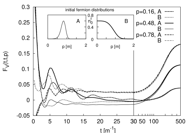
Figure 2: The time evolution of the fermion two-point function $F_{V}(t,t;p)$ for three values of the momentum $p$, in units of the renormalized scalar thermal mass $m$. The evolution is shown for two very different initial conditions with the same initial energy density. One observes that the dynamics becomes rather quickly insensitive to the initial distributions displayed in the insets – much before the modes settle to their final values. The long-time behavior is shown on a logarithmic scale for $t\geq 30m^{-1}$.

In Fig. 2 we present the time evolution of the fermion equal-time two-point function $F_{V}(t,t;p)$ for three momenta $p$. Results are given for two very different initial particle number distributions, which are displayed in the insets (see also Eqs. (7.54)–(7.56)). The (conserved) energy density is taken to be the same for both runs. In this case, since thermal equilibrium is uniquely specified by the value of the energy density, the correlator modes should approach universal values at late times if thermalization occurs.

Figure 3: The same as in Fig. 2 but for the bosonic two-point function $F_{\phi}(t,t;p)$ for three different momenta. The initial particle number distributions for the two runs denote by “A” and “B” are displayed in the insets. For the employed parameters one observes that, in the scalar sector, the time needed to become effectively insensitive to the initial distributions is comparable to the time scale describing the approach to the universal late-time value.

It is striking to observe from Fig. 2 that after a comparably short time, much before the correlation modes reach their late-time values, the dynamics becomes rather insensitive to the details of the initial conditions: for a given momentum, the curves corresponding to the two different runs come close to each other rather quickly. During the slow subsequent evolution the system is still far away from equilibrium before the approach to the late-time values sets in. From both runs one observes that the characteristic time needed to effectively loose the information about the details of the initial conditions is much shorter than the time needed to approach the late-time result. Moreover, the late-time values are found to be universal in the sense that the different runs agree with each other to very good precision.

Fig. 3 shows the corresponding behavior of the scalar correlator modes $F_{\phi}(t,t;p)$. The respective initial particle number distributions in the scalar sector for the two runs are given in the inset. For the two different runs the modes having the same momenta approach each other rather slowly as compared to the fermionic sector. However, they reach their final values on a time scale which is comparable to that observed for the fermions in Fig 2.

Figure 4: The fermionic two-point function $F_{V}(t,t^{\prime};p)$ as a function of $t-t^{\prime}$ at late time $t=600\,m^{-1}$. One observes a very good agreement with an exponential behavior. The rate is well described by the width of the corresponding spectral function in frequency space as shown in the inset (cf. the text for details).

To characterize these time scales in more detail, we consider in Fig. 4 the unequal-time two-point function $F_{V}(t,t^{\prime};p)$. As expected, if the system is to become insensitive to the details of the initial conditions, we observe that the correlation between some time $t$ and another time $t^{\prime}$ is suppressed for sufficiently large $t-t^{\prime}$. We note that the oscillation envelope of $F_{V}(t,t^{\prime},p)$ can be well described in terms of an exponential for sufficiently late times. The corresponding damping rate approaches a constant value. To estimate the asymptotic rate we show in Fig. 4 the unequal-time two-point function $F_{V}(t,t^{\prime};p)$ as a function of $t-t^{\prime}$ for the late time $mt=600$. The fit to an exponential yields the damping rate $\gamma^{\rm(damp)}_{f}(p=0.78m)=0.03(1)\,m$. We find a moderate momentum dependence of this rate with $\gamma^{\rm(damp)}_{f}(0)=0.067(1)m$ and $\gamma^{\rm(damp)}_{f}(0)\gtrsim\gamma^{\rm(damp)}_{f}(p>0)$.

We emphasize that the rate $\gamma^{\rm(damp)}_{f}(p)$ can be related to the width of the Fourier transform of the spectral function with respect to the time difference $t-t^{\prime}$. In principle, the latter involves an integration over an infinite time interval. However, since we consider an initial-value problem for finite times we know $\rho_{V}(t,t^{\prime},p)$ only on a finite interval. To overcome this problem, we fit the data for $\rho_{V}(t,t^{\prime},p)$ by a $7$–parameter formula that is capable to account for the observed oscillations and damping, but which is more general than the usual 2-parameter Breit-Wigner formula. We perform the Fourier transformation on the extrapolated data. The resulting function $\rho_{V}(\omega,p)$ is displayed as a function of frequency $\omega$ in the inset of Fig. 4. One clearly observes a nonzero width of the spectral function, the value of which may be obtained from a fit to a Breit-Wigner formula. By doing so, we obtain a very good agreement of the damping rate inferred from the width of the spectral function on the one hand and from the linear fit on the log-plot for $F_{V}(t,t^{\prime};p)$ on the other hand.

We can use the fermion damping rate to quantify the time scale characterizing the effective loss of the details of the initial conditions: Comparing with Fig. 2, we observe that the inverse fermion damping rate at $p\simeq 0$ $\left(1/\gamma^{\rm(damp)}_{f}=15(1)m^{-1}\right)$ characterizes well the time for which the dynamics becomes rather insensitive to the initial distributions. In contrast, we find that this time scale does not characterize the late-time behavior. For the latter, we observe to very good approximation an exponential relaxation of each mode $F_{V}(t,t;p)$ to its universal late-time value. Carrying out the measurement for different modes, we observe that the corresponding rate is almost independent of momentum and is given by $1/\gamma^{\rm(therm)}_{f}=95(5)m^{-1}$. The corresponding time scale $1/\gamma^{\rm(therm)}_{f}$ is therefore much larger than the characteristic damping time $1/\gamma^{\rm(damp)}_{f}$.

A similar analysis can be performed for the scalar sector. Here we find at $p\simeq 0$ the corresponding values $1/\gamma^{\rm(damp)}_{\phi}=50(5)\,m^{-1}$ and $1/\gamma^{\rm(therm)}_{\phi}=90(5)m^{-1}$. One observes that although the damping rates for fermions and bosons are very different, the respective thermalization rates are rather similar. For the scalars the thermalization rate is larger than the damping rate, as is observed above for the fermions. However, the difference is much less pronounced for the scalars. Similar studies in $1+1$ dimensional quantum [9] and classical [8] scalar theories typically find a substantial difference between damping and thermalization rates. However, this may be a consequence of the stringent phase-space restrictions and therefore particular to $1+1$ dimensional systems.

We finally note that approximate rates describing the early-time behavior may be determined by an exponential fit to the functions $F_{\phi}(t,0)$, $F_{V}^{0}(t,0)$ and $F_{V}(t,0)$ in a finite time interval. These rates depend on time and approach the late-time values given above. At early times we observe an approximate exponential damping with a rate about twice as big as the late-time value for the fermions, and about half the late-time rate for the scalars.

10 Approach to quantum thermal equilibrium

In the previous section, we have seen that the out-of-equilibrium evolution of the system leads to a universal late-time behavior, uniquely characterized by the initial energy density. We now analyze in detail if quantum thermal equilibrium, characterized by Bose-Einstein and Fermi-Dirac statistics, is approached. In thermal equilibrium, the spectral function and the statistical two-point function are not independent of each other, but are related by the fluctuation-dissipation relation. The latter is an exact relation, which can be stated in $4$–dimensional Fourier space as [9, 22]

$$F^{(\rm eq)}_{\phi}(\omega,\vec{p})=-i\left(n^{BE}(\omega)+\frac{1}{2}\right)\rho^{(\rm eq)}_{\phi}(\omega,\vec{p})\,,$$ (10.57)

for the scalar correlators, where $n^{BE}(\omega)=1/[\exp(\omega/T)-1]$ denotes the Bose–Einstein distribution function. The frequency $\omega$ is the Fourier conjugate of $t-t^{\prime}$ (in thermal equilibrium, time-translation invariance implies that two-point functions only depend on $t-t^{\prime}$). The value of the temperature $T$ is determined by the energy density of the system. The fluctuation-dissipation relation for the fermion correlators is given by the equivalent expression with the replacement $(n^{BE}(\omega)+\frac{1}{2})\to(n^{FD}(\omega)-\frac{1}{2})$ in Eq. (10.57) and the Fermi–Dirac distribution $n^{FD}=1/[\exp(\omega/T)+1]$. The same relations hold as well for the statistical and spectral components of the self-energies in thermal equilibrium. They provide an unambiguous way to extract the distribution functions, which are specific for quantum thermal equilibrium. Out of equilibrium, the spectral and statistical two-point functions are completely independent in general. However, if thermal equilibrium is approached at late times, they become related by the fluctuation-dissipation relations.

Figure 5: The late-time ratio of the statistical two-point function and the spectral function in frequency space, both for fermions ($F_{V}/\rho_{V}$) and for scalars ($F_{\phi}/\rho_{\phi}$). In thermal equilibrium the quotient corresponds to the Bose-Einstein (BE) distribution function for scalars and to the Fermi-Dirac (FD) distribution for fermions – independently of any assumption on a quasi-particle picture (see Eq. (10.57)). The BE/FD distributions are displayed by the continuous curves parametrized by the same temperature. The value of the latter, $T=0.94m$, is actually not fitted but has been taken from the inverse slope of Fig. 8. This shows the correspondence with the quasi-particle picture described in the text.

To extract the answer about the late-time distributions, without relying on any assumptions, we consider the statistical and spectral correlators in Wigner coordinates. For this we express $F_{\phi}(t,t^{\prime};p)$ and $\rho_{\phi}(t,t^{\prime};p)$, as well as the corresponding fermion two-point functions, in terms of the center coordinate $X^{0}=(t+t^{\prime})/2$ and the relative coordinate $s^{0}=t-t^{\prime}$ and write

$$\rho_{\phi}(X^{0};\omega,p)=\int_{-2X^{0}}^{2X^{0}}{\rm d}s^{0}\,e^{i\omega s^{0}}\,\rho_{\phi}(X^{0}+s^{0}/2,X^{0}-s^{0}/2;p)\,,$$ (10.58)

and equivalently for the other correlators. Since we consider an initial-value problem, the time integral over $s^{0}$ is bounded by $\pm 2X^{0}$ (cf. also the detailed discussion in Ref. [22]). If thermal equilibrium is approached for sufficiently large $X^{0}$, then the correlators do no longer depend on $X^{0}$ and a Fourier transform with respect to $t-t^{\prime}$ can be performed to very good approximation (cf. the discussion in Sect. 9). The distribution functions may then be extracted from the quotient of the Wigner transformed two-point functions. In Fig. 5 we show the respective ratios at late times. Both functions are in good agreement with the equilibrium distributions $n^{FD}(\omega)$ and $n^{BE}(\omega)$, respectively (cf. Eq. (10.57)). We emphasize that the displayed continuous curves are no separate fits. They are the Bose-Einstein and Fermi-Dirac distribution functions parametrized by the same temperature. In particular, the value for the temperature is not fitted but has been extracted from the inverse slope parameter as explained below.

Figure 6: The time-dependent fermion quasi-particle distribution $n_{f}(t,p)$ as a function of mode energy $p$ for various times $t$. We have plotted the inverse slope function $\log(1/n_{f}-1)$, which reduces to a straight line intersecting the origin when $n_{f}(t,p)$ approaches a Fermi-Dirac distribution. This plot shows the data for run “A” of Fig. 2.

We stress that the above procedure to extract the distribution functions is independent of any assumption about a quasi-particle picture. However, for many practical purposes it is very convenient to have an effective description of particle number and mode energy directly in real time – without the need of a Fourier transform. An efficient description is elaborated in Appendix A. The value for the temperature in the thermal equilibrium distributions of Fig. 5 has been actually measured based on this quasi-particle picture. In Appendix A we define the effective particle number and energy to be used, both for the fermionic and bosonic fields. For scalar field theories, this quasi-particle picture has been successfully employed previously to investigate thermalization [9, 28, 22].

Figure 7: The time-dependent boson quasi-particle distribution $n(t,p)$ as a function of mode energy $\epsilon(t,p)$ (see text) for various times. In this case the inverse slope function is $\log(1/n+1)$, which reduces to a straight line in case of a Bose-Einstein distribution. This plot shows the data for run “A” of Fig. 3.

In Figs. 6 and 7 we show the effective quasi-particle number distributions defined as

$$\frac{1}{2}-n_{f}(t,p)=F_{V}(t,t;p)$$ (10.59)

for fermions and

$$\frac{1}{2}+n(t,p) = \epsilon(t,p)\,F_{\phi}(t,t;p)\,,$$ (10.60)

$$\epsilon(t,p) = \left(\frac{\partial_{t}\partial_{t^{\prime}}F_{\phi}(t,t^{\prime};p)}{F_{\phi}(t,t^{\prime};p)}\right)_{t=t^{\prime}}^{1/2}$$ (10.61)

for scalars, where $\varepsilon(t,p)$ is the quasi-particle mode energy as discussed in Appendix A. The curves correspond to the initial conditions of run “A” shown in Figs. 2 and 3.

Figure 8: Boson and fermion quasi-particle distributions at late times as a function of mode energy ($n_{p}\equiv n(t,p)$ and $\epsilon_{p}\equiv\epsilon(t,p)$ for bosons and $n_{p}\equiv n_{f}(t,p)$ and $\epsilon_{p}\equiv p$ for fermions). Both inverse slope functions employed in Figs. 6 and 7 have been applied here in order to demonstrate that the fermions clearly do not follow a Bose-Einstein distribution, and the scalars cannot be characterized by a Fermi-Dirac distribution. In contrast, for the respective correct statistics the curves lie on top of each other, showing that both fermions and scalars are described by the same inverse slope parameter. The value of the latter is used in Fig. 5 as the temperature for the distributions $n^{FD}(\omega)$ and $n^{BE}(\omega)$.

One observes how the effective fermion and boson particle numbers change with time, the former approaching a Fermi–Dirac and the latter a Bose–Einstein distribution. To emphasize this point, we plot the corresponding “inverse slope functions” $\log(1/n_{f}-1)$ and $\log(1/n+1)$, which reduce to straight lines for Fermi–Dirac and Bose–Einstein distributions respectively. The associated inverse slopes correspond to the temperature of the thermal equilibrium distributions. We see in Figs. 6 and 7 that both inverse slope functions approach straight lines at late times. The associated temperatures for fermions and bosons are independent of time and agree very well with each other, as shown in Fig. 8. For comparison, we display in Fig. 8 the fermion inverse slope function evaluated with the bosonic effective particle number, and vice versa. This illustrates the degree of sensitivity of the inverse slope functions to the different statistics and in turn the degree of precision with which we are able to probe thermalization.

11 Conclusions

In this paper we have discussed the far-from-equilibrium dynamics and subsequent thermalization of a system of coupled fermionic and bosonic quantum fields. We solved the nonequilibrium dynamics beyond mean-field type approximations by calculating the complete lowest non-trivial order in a systematic coupling expansion of the 2PI effective action, which includes direct scattering as well as memory and off-shell effects. To our knowledge this is the first time that such a calculation is performed without further approximations. As a result, we show that, for various far-from-equilibrium initial conditions, the late-time behavior is universal and uniquely determined by the value of the initial energy density. Moreover, we are able to probe the approach to quantum thermal equilibrium, characterized by the emergence of Fermi–Dirac and Bose–Einstein distribution functions, with high accuracy. We emphasize that in the present calculation, besides the limitations of a coupling expansion, there is no other input than the dynamics dictated by the considered quantum field theory for given nonequilibrium initial conditions.

This work can be extended in many directions. Most of the equations we derive are also valid in the phase with spontaneous symmetry breaking. Combined with earlier work on scalar theories [9, 11, 26], this provides a description of the nonequilibrium dynamics of the linear $\sigma$-model for QCD with two quark flavors. The model has served for many years as a valuable testing ground for ideas on the equilibrium phase structure of low energy QCD at nonzero temperature and density. With the present techniques a quantitative understanding of the out-of-equilibrium physics of this model is within reach.

Acknowledgment

We thank C. Wetterich for many discussions and collaboration on related work. We are also grateful to W. Wetzel for his continuous support with computers. Sz. B. acknowledges the hospitality of the Institute für Theoretische Physik, Heidelberg. His work was supported by the short-term scholarship program of the DAAD.

Appendix A Effective particle number and energy

A particle number can only be strictly defined in the presence of a conserved charge. However, for physical interpretation it is often convenient to define an effective particle number even when there is no conserved charge. In particular, besides a total particle number it is often useful to have a definition of an effective particle number per (momentum) mode. The latter is typically not conserved in an interacting theory, and in the context of thermalization one would like to find a time-dependent particle number distribution, which allows one to observe a Bose-Einstein or Fermi-Dirac distribution at sufficiently late times. Of course, the notion of an effective particle number is typically only meaningful if the relevant degrees of freedom or “quasi-particles” are weakly interacting.

There are many different ways of how one can introduce the notion of an effective particle number (for a recent discussion see e.g. Ref. [29] and references therein). For example, one can define it as the average energy per mode divided by the energy of the corresponding mode. In an interacting theory, this procedure can be ambiguous because the expression of the total energy receives contributions from interactions and the average energy per mode is not uniquely defined. In this appendix, we discuss an elegant way to circumvent this difficulty. More importantly for our purposes, the procedure leads to a definition of an effective particle number density, which indeed allows one to directly observe the emergence of a Fermi-Dirac or Bose-Einstein distribution from the nonequilibrium dynamics for the theory considered in this paper. In particular, it can be explicitely shown that the effective particle numbers are always positive and, for the fermions, smaller than one (see Appendix B). Applying the present construction to the case of neutral scalar fields, we recover the particle number definition used in previous studies to exhibit thermalization in purely scalar field theories [22, 9].

Fermions

We start by considering the case of charged fields and construct the effective particle number from the conserved current generated by the $U(1)$ symmetry. The associated $4$–current for each given flavor is $\sim\bar{\psi}\gamma^{\mu}\psi$. Fourier transformed with respect to spatial momenta, the expectation value of the latter can be written as $J_{f}^{\mu}(t,p)=\hbox{tr}[\gamma^{\mu}D^{<}(t,t,p)]$, where the subscript stands for fermions (cf. Eq. (3.8)). In terms of the equal-time statistical two point function, its temporal and spatial components read:

$$J_{f}^{0}(t,p) = 2\,[1-2\,F_{V}^{0}(t,t;p)]\,,$$

$$\vec{J}_{f}(t,p) = -4{\vec{v}}\,F_{V}(t,t;p)\,.$$

A nice property is that the above expressions in terms of the full correlators do not contain any explicit dependence on the interaction part. In order to obtain an effective particle number, we want to identify these expressions with the corresponding ones in a quasi-particle description with free-field expressions. These are given by:

$$J_{f}^{0\,({\rm QP})}(t,p) = 2\,[1+Q_{f}(t,p)]\,,$$

$$\vec{J}_{f}^{\,({\rm QP})}(t,p) = -2{\vec{v}}\,[1-2N_{f}(t,p)]\,,$$

where $Q_{f}(t,p)=n_{f}-\bar{n}_{f}$ is the difference between particle and anti-particle effective number densities and $N_{f}(t,p)=(n_{f}+\bar{n}_{f})/2$ is their half-sum. The physical content of these expressions is simple: the temporal component $J^{0}$ directly represents the net-charge density per mode $Q_{f}(t,p)$, whereas the spatial part $\vec{J}$ is the net current density per mode and is therefore sensitive to the sum of particle and anti-particle number densities. Identifying the above expressions, we define

$$\frac{1}{2}\,Q_{f}(t,p) = -F_{V}^{0}(t,t;p)\,,$$ (A.62)

$$\frac{1}{2}-N_{f}(t,p) = F_{V}(t,t;p)\,.$$ (A.63)

Of course, these expressions are only meaningful for the case that the interacting theory is well-described by a quasi-particle picture. The important point is that the above procedure allows one to construct an effective particle number density without knowing a priori which part of the interaction is to be considered as the “dressing” of the quasi-particles and which part describe their “residual” interactions. We note that the equal-time two-point functions on the RHS of these equations are real by definition (see Eq. (5.32)). Moreover, using the anticommutation relation for the fermion fields, it is shown in Appendix B that these definitions always satisfy $0\leq N_{f}(t,p)\leq 1$ and $-1\leq Q_{f}(t,p)\leq 1$. These properties are important for the above definitions to be physically meaningful.

Introducing a non-vanishing net charge density per mode was useful for the above general construction. However, in the present paper, we consider only $CP$–invariant systems, which imply that the latter should vanish. Indeed, we see from Eqs. (5.32) that the requirement of $CP$–invariance imply that our above definition of net charge density per mode vanishes identically for all times and for all modes. Therefore, the effective particle and anti-particle numbers are equal and we have

$$Q_{f}(t,p) = 0\,,$$

$$\frac{1}{2}-n_{f}(t,p) = F_{V}(t,t;p)\,.$$

where $n_{f}(t,p)$ is the effective particle number.

Bosons

Following the same lines as above, let us consider for a moment the case of a single charged scalar field $\phi$. The $4$-current associated the corresponding $U(1)$ symmetry is $\sim i[\phi^{\dagger}(\partial^{\mu}\phi)-(\partial^{\mu}\phi^{\dagger})\phi]$ and, as for the case of fermions, its expectation value has a simple expression in terms of the equal-time statistical two-point function of the charged field. In momentum space, it reads:

$$J_{b}^{0}(t,p) = i(\partial_{t}-\partial_{t^{\prime}})\,F_{\phi}(t,t^{\prime};p)|_{t^{\prime}=t}-1\,,$$

$$\vec{J}_{b}(t,p) = 2\,{\vec{p}}\,F_{\phi}(t,t;p)\,,$$

where, as before, the constant contribution comes from the fact that we define the current without the usual normal ordering. Here, the statistical two-point function for the charged scalar field is defined as the expectation value of the anticommutator of two fields operators: $F_{\phi}(t,t^{\prime};p)=\mbox{$\frac{1}{2}\langle[\phi(t,{\vec{p}}),\phi^{\dagger}(t^{\prime},{\vec{p}})]_{+}\rangle$}$. It has the symmetry property $F_{\phi}(t,t^{\prime};p)=F_{\phi}^{*}(t^{\prime},t;p)$, so that the above expressions are real. The corresponding quasi-particle expressions read:

$$J_{b}^{0\,({\rm QP})}(t,p) = Q_{b}(t,p)-1\,,$$

$$\vec{J}_{b}^{\,({\rm QP})}(t,p) = \frac{{\vec{p}}}{\epsilon(t,p)}\,[1+2N_{b}(t,p)]\,,$$

where $Q_{b}(t,p)$ and $N_{b}(t,p)$ have the same meaning as before in terms of effective particle and anti-particle number densities and where $\epsilon(t,p)$ is the quasi-particle energy. We therefore define:

$$Q_{b}(t,p) = i(\partial_{t}-\partial_{t^{\prime}})\,F_{\phi}(t,t^{\prime};p)|_{t^{\prime}=t}\,,$$ (A.64)

$$1+2N_{b}(t,p) = 2\,\epsilon(t,p)\,F_{\phi}(t,t;p)\,.$$ (A.65)

Note that the RHS of both expressions are real quantities, as they should if the LHS are to be interpreted as charge and quasi-particle number densities respectively.

It remains to define the effective quasi-particle energy $\epsilon(t,p)$. For this purpose, we use the free-field like expression for the average energy per mode, which in the case of a single charged scalar field can be written as

$$\partial_{t}\partial_{t^{\prime}}F_{\phi}(t,t^{\prime};p)|_{t^{\prime}=t}+\epsilon^{2}(t,p)F_{\phi}(t,t;p)\equiv\epsilon(t,p)\,\Big{[}2n(t,p)+1\Big{]}\,$$

in terms of the statistical two-point function. Therefore, one obtains for the effective quasi-particle energy:

$$\epsilon^{2}(t,p)=\left(\frac{\partial_{t}\partial_{t^{\prime}}F_{\phi}(t,t^{\prime};p)}{F_{\phi}(t,t^{\prime};p)}\right)_{t=t^{\prime}}\,.$$ (A.66)

It is straightforward to show that the combination of equal-time correlators appearing on the RHS of (A.66) is indeed positive. Moreover, using commutation relations for the scalar field, one can show that the effective particle number $N_{b}(t,p)$, as given by Eqs. (A.65) and (A.66), is a positive quantity (see Appendix B). We note that for the case of $CP$–invariant systems, the effective charge density per mode (A.64) vanishes, as it should.

When dealing with neutral scalar fields, as it is the case in the present paper, we can use the same formula derived above. Notice that this is consistent since in that case one has $F_{\phi}(t,t^{\prime};p)=F_{\phi}(t^{\prime},t;p)$, which directly implies that $Q_{b}(t,p)=0$. Therefore, in the present paper, we use the definition

$$\frac{1}{2}+n(t,p)=\epsilon(t,p)\,F_{\phi}(t,t;p)\\$$ (A.67)

together with (A.66) for the boson effective particle number $n(t,p)$ and mode energy $\epsilon(t,p)$ for each individual scalar species [22, 9].

Appendix B

Here we show that the combinations of equal-time two-point functions used in this paper to define effective particle number densities are always positive and, for the fermionic case, smaller than one. It is demonstrated to be a simple consequence of the (anti-)commutation relations of field operators.

Fermions

As a first exercise, we show that for any operators $\varphi$ and $\varphi^{\dagger}$ satisfying the anticommutation relations

$$[\varphi,\varphi^{\dagger}]_{{}_{{}_{+}}}=1$$

and

$$[\varphi,\varphi]_{{}_{+}}=[\varphi^{\dagger},\varphi^{\dagger}]_{{}_{+}}=0\,,$$

one has

$$0\,\leq\,\langle\varphi^{\dagger}\,\varphi\rangle\,\leq\,1\,,$$ (B.68)

where the brackets denote an average with respect to any density matrix. The left inequality above is trivially obtained for example by inserting a complete sum of states between the operators $\varphi^{\dagger}$ and $\varphi$. One obtains a sum of positive quantities which is of course positive. To show the second inequality, we introduce the hermitian operator $N=\varphi^{\dagger}\varphi$. Using the anticommutation relations above, it is easy to see that $N^{2}=N$, from which it follows that

$$\Delta n^{2}\equiv\Big{\langle}\,\Big{(}N-\langle N\rangle\Big{)}^{2}\,\Big{\rangle}=\langle N^{2}\rangle-\langle N\rangle^{2}=\langle N\rangle\Big{(}1-\langle N\rangle\Big{)}\,.$$

It is clear that $\Delta n^{2}\geq 0$ and we have just shown that $\langle N\rangle\geq 0$. One therefore conclude from the above equation that $\langle N\rangle\leq 1$, as announced.

We now come to our effective particle number densities. Using Eqs. (A.62) and (A.63) and recalling that $Q_{f}\equiv n_{f}-\bar{n}_{f}$ and $N_{f}\equiv(n_{f}+\bar{n}_{f})/2$, we get for the effective particle and anti-particle number densities:

$$\frac{1}{2}-n_{f}(t,p) = F_{V}(t,t,p)+F_{V}^{0}(t,t,p)=\frac{1}{4}\hbox{tr}\Big{[}(\gamma_{0}+{\vec{v}}\cdot\vec{\gamma})F(t,t,p)\Big{]}\,,$$

$$\frac{1}{2}-\bar{n}_{f}(t,p) = F_{V}(t,t,p)-F_{V}^{0}(t,t,p)=-\frac{1}{4}\hbox{tr}\Big{[}(\gamma_{0}-{\vec{v}}\cdot\vec{\gamma})F(t,t,p)\Big{]}\,.$$

In terms of the fermionic field operators $\psi(t,{\vec{p}})$ and $\bar{\psi}(t,{\vec{p}})$, which satisfy the anticommutation relations

$$[\psi(t,{\vec{p}}),\bar{\psi}(t,{\vec{p}})]_{{}_{+}}=\gamma_{0}$$

and

$$[\psi(t,{\vec{p}}),\psi(t,{\vec{p}})]_{{}_{+}}=[\bar{\psi}(t,{\vec{p}}),\bar{\psi}(t,{\vec{p}})]_{{}_{+}}=0\,,$$

one has

$$F(t,t,p)=\frac{1}{2}\Big{\langle}[\psi(t,{\vec{p}}),\bar{\psi}(t,{\vec{p}})]_{{}_{-}}\Big{\rangle}\,.$$

Therefore, one can rewrite (from now on, we drop the explicit $t$ and ${\vec{p}}$ dependence):

$$n_{f} = \frac{1}{4}\,\langle\bar{\psi}(\gamma_{0}+{\vec{v}}\cdot\vec{\gamma})\psi\rangle\,,$$

$$1-\bar{n}_{f} = \frac{1}{4}\,\langle\bar{\psi}(\gamma_{0}-{\vec{v}}\cdot\vec{\gamma})\psi\rangle\,.$$

Now we introduce the operator

$$\varphi=\frac{\gamma_{0}+{\vec{v}}\cdot\vec{\gamma}}{\sqrt{2}}\,\psi\,,$$

in term of which,

$$n_{f}=\frac{1}{4}\,\sum_{\alpha=1}^{4}\langle\varphi^{\dagger}_{\alpha}\varphi_{\alpha}\rangle\,,$$ (B.69)

where we explicitely wrote the sum over Dirac indices. For a given Dirac index, it is straightforward to check that

$$[\varphi_{\alpha},\varphi^{\dagger}_{\alpha}]_{{}_{{}_{+}}}=\Big{(}1-\gamma_{0}\,{\vec{v}}\cdot\vec{\gamma}\Big{)}_{\alpha\alpha}=1$$ (B.70)

and

$$[\varphi_{\alpha},\varphi_{\alpha}]_{{}_{+}}=[\varphi^{\dagger}_{\alpha},\varphi^{\dagger}_{\alpha}]_{{}_{+}}=0\,,$$

where we specialized to the Dirac basis to write the last equality of Eq. (B.70). Using (B.68) for each individual $\alpha$, we conclude from (B.69) that

$$0\leq n_{f}(t,p)\leq 1$$

for any time $t$ and any momentum $p$. It is straightforward to repeat the above arguments to show that

$$0\leq\bar{n}_{f}(t,p)\leq 1\,.$$

Bosons

For scalars, we first use Eqs. (A.66) and (A.66) to rewrite

$$\frac{1}{2}+n(t,p)=\sqrt{F_{\phi}(t,t;p)\,[\partial_{t}\partial_{t^{\prime}}F_{\phi}(t,t^{\prime};p)]_{t^{\prime}=t}}\,.$$

Recalling the definition of the statistical propagator in terms of field operators:

$$F_{\phi}(t,t;p) = \langle\phi^{\dagger}(t,{\vec{p}})\,\phi(t,{\vec{p}})\rangle\,,$$

$$\partial_{t}\partial_{t^{\prime}}F_{\phi}(t,t^{\prime};p)]_{t^{\prime}=t} = \langle\Pi^{\dagger}(t,{\vec{p}})\,\Pi(t,{\vec{p}})\rangle\,,$$

where $\Pi(t,{\vec{p}})$ and $\Pi^{\dagger}(t,{\vec{p}})$ are the canonical momenta conjugate to $\phi^{\dagger}(t,{\vec{p}})$ and $\phi(t,{\vec{p}})$ respectively (e.g. $\Pi(t,{\vec{p}})=\dot{\phi}^{\dagger}(t,{\vec{p}})$), we see that

$$n(t,p)\geq 0\,\,<=>\,\,\langle\phi^{\dagger}\,\phi\rangle\,\langle\Pi^{\dagger}\,\Pi\rangle\geq\frac{1}{2}\,,$$

where we dropped in the notation the explicit time and momentum dependence of field operators. The second inequality is nothing but Heisenberg’s uncertainty relation, a direct consequence of the equal-time canonical commutation relations of field operators [33].

References

- [1] P. Braun-Munzinger and J. Stachel, J. Phys. G 28 (2002) 1971; U. W. Heinz and P. F. Kolb, “Two RHIC puzzles: Early thermalization and the HBT problem”, arXiv:hep-ph/0204061, Proceedings of the 18th Winter Workshop on Nuclear Dynamics. Edited by R. Bellwied, J. Harris, and W. Bauer. EP Systema, Debrecen, Hungary, 2002. pp. 205-216.
- [2] J. Serreau, Proceedings of Quark Matter 2002, to appear in Nucl. Phys. A [arXiv:hep-ph/0209067]; J. Serreau and D. Schiff, JHEP 0111 (2001) 039; R. Baier, A. H. Mueller, D. Schiff and D. T. Son, Phys. Lett. B 539 (2002) 46.
- [3] For a review see J. P. Blaizot and E. Iancu, Phys. Rept. 359 (2002) 355, and references therein; see also: P. Arnold, G. D. Moore and L. G. Yaffe, JHEP 0301 (2003) 030.
- [4] F. Cooper, S. Habib, Y. Kluger, E. Mottola, J.P. Paz, P.R. Anderson, Phys. Rev. D50 (1994) 2848; D. Boyanovsky, H. J. de Vega, R. Holman, J. Salgado, Phys. Rev. D59 (1999) 125009.
- [5] F. Cooper and V. M. Savage, Phys. Lett. B 545 (2002) 307; A. Chodos, F. Cooper, W. Mao and A. Singh, Phys. Rev. D 63 (2001) 096010; D. Boyanovsky, H. J. De Vega, R. Holman and M. R. Martin, Phys. Rev. D 65 (2002) 045007.
- [6] J. Baacke, K. Heitmann and C. Pätzold, Phys. Rev. D 58 (1998) 125013; J. Baacke and C. Pätzold, Phys. Rev. D 62 (2000) 084008.
- [7] F. Cooper, S. Habib, Y. Kluger and E. Mottola, Phys. Rev. D 55 (1997) 6471.
- [8] G. Aarts, G. F. Bonini and C. Wetterich, Phys. Rev. D 63 (2001) 025012.
- [9] J. Berges, Nucl. Phys. A 699 (2002) 847.
- [10] J. Berges and J. Cox, Phys. Lett. B 517 (2001) 369.
- [11] G. Aarts, D. Ahrensmeier, R. Baier, J. Berges and J. Serreau, Phys. Rev. D 66 (2002) 045008
- [12] J. M. Luttinger and J. C. Ward, Phys. Rev. 118 (1960) 1417; G. Baym, Phys. Rev. 127 (1962) 1391.
- [13] J. M. Cornwall, R. Jackiw and E. Tomboulis, Phys. Rev. D 10 (1974) 2428.
- [14] E. Calzetta and B. L. Hu, Phys. Rev. D 37 (1988) 2878.
- [15] Y. B. Ivanov, J. Knoll and D. N. Voskresensky, Nucl. Phys. A 657 (1999) 413.
- [16] For reviews, see P. Danielewicz, Annals Phys. 152 (1984) 239; for relativistic fermions, see also H. T. Elze and U. W. Heinz, Phys. Rept. 183 (1989) 81; D. A. Brown and P. Danielewicz, Phys. Rev. D 58 (1998) 094003.
- [17] P. B. Greene and L. Kofman, Phys. Rev. D 62 (2000) 123516.
- [18] M. Joyce, K. Kainulainen and T. Prokopec, JHEP 0010 (2000) 029; K. Kainulainen, T. Prokopec, M. G. Schmidt and S. Weinstock, Phys. Rev. D 66 (2002) 043502.
- [19] I. D. Lawrie and D. B. McKernan, Phys. Rev. D 62 (2000) 105032.
- [20] G. Aarts and J. Smit, Nucl. Phys. B 555 (1999) 355.
- [21] J. Schwinger, J. Math. Phys. 2 (1961) 407; L. V. Keldysh, Zh. Eksp. Teor. Fiz. 47 (1964) 1515 [Sov. Phys. JETP 20 (1965) 1018]; K. C. Chou, Z. B. Su, B. L. Hao and L. Yu, Phys. Rept. 118 (1985) 1.
- [22] G. Aarts and J. Berges, Phys. Rev. D 64 (2001) 105010.
- [23] J. Berges, N. Tetradis and C. Wetterich, Phys. Rept. 363 (2002) 223.
- [24] I. Montvay, G. Münster, “Quantum Fields on a Lattice”, Cambridge University Press, 1994.
- [25] K. Kainulainen, T. Prokopec, M. G. Schmidt, S. Weinstock, COSMO-01, hep-ph/0201245.
- [26] J. Berges and J. Serreau, arXiv:hep-ph/0208070.
- [27] G. Aarts, J. Smit, Phys. Rev. D61 (2000) 025002; M. Salle, J. Smit and J. C. Vink, Nucl. Phys. B 625 (2002) 495; L. M. Bettencourt, K. Pao and J. G. Sanderson, Phys. Rev. D 65 (2002) 025015.
- [28] G. Aarts and J. Berges, Phys. Rev. Lett. 88 (2002) 041603.
- [29] B. Garbrecht, T. Prokopec and M. G. Schmidt, arXiv:hep-th/0211219.
- [30] M. Gell-Mann and M. Levy, Nuovo Cim. 16 (1960) 705.
- [31] See e.g. R. D. Pisarski and F. Wilczek, Phys. Rev. D 29 (1984) 338; J. Berges, D. U. Jungnickel and C. Wetterich, Phys. Rev. D 59 (1999) 034010; O. Scavenius, A. Mocsy, I. N. Mishustin and D. H. Rischke, Phys. Rev. C 64 (2001) 045202.
- [32] L. M. Bettencourt and C. Wetterich, Phys. Lett. B 430 (1998) 140.
- [33] Arno Bohm, “Quantum Mechanics: Foundations and Applications”, Springer-Verlag, Heidelberg, 1994.