Prospective Analysis of Spin- and CP-sensitive Variables in H $\rightarrow$ ZZ $\rightarrow$ l${}^{+}_{1}$l${}^{-}_{1}$l${}^{+}_{2}$l${}^{-}_{2}$ with Atlas

Abstract

A possibility to prove spin and CP-eigenvalue of a Standard Model (SM) Higgs boson is presented. We exploit angular correlations in the subsequent decay H $\rightarrow$ ZZ $\rightarrow$ 4l (muons or electrons) for Higgs masses above 200 GeV. We compare the angular distributions of the leptons originating from the SM Higgs with those resulting from decays of hypothetical particles with differing quantum numbers. We restrict our analysis to the use of the Atlas-detector which is one of two multi-purpose detectors at the upcoming 14 TeV proton-proton-collider (LHC) at CERN. By applying a fast simulation of the Atlas detector it can be shown that these correlations will be measured sufficiently well that consistency with the spin-CP hypothesis 0+ of the Standard Model can be verified and the 0- and 1$\pm$ can be ruled out with an integrated luminosity of 100 fb^-1.

Freiburg-THEP 02/16

1 Introduction

Although the standard $SU(2)_{L}\times U(1)_{Y}$ electroweak gauge theory successfully explains all current electroweak data, the mechanism of spontaneous symmetry breaking has been tested only partially. Since in the Standard Model spontaneous symmetry breaking is due to the Higgs Mechanism, the search for a Higgs particle will be one of the main tasks of future colliders.

At present, LEP gives a lower limit of 114.4 GeV/c² [1] for the Higgs boson mass. There is also an indirect upper limit from electroweak precision measurements of 219 GeV/c² at a 95% confidence level [2] which is valid in the minimal standard model. However, this limit is still preliminary and the quality of the SM fit, when including all EW measurements from both low and high energy experiments, is still an object of discussion amongst experts [3]. Furthermore, a heavier Higgs boson would be consistent with the electroweak precision measurements in models more general than the minimal standard model [4]. In this first analysis we will therefore also consider higher Higgs masses well above this limit, as can be produced at high energy hadron colliders such as the LHC (pp collisions at 14 TeV). A Standard Model Higgs boson lying below the $WW$ threshold will mainly decay into a $b\bar{b}$ pair. In this case, there is an overwhelming direct QCD background which dominates the signal. Therefore, the Higgs boson is difficult to study in detail in this mass region, even though one can use rare decays as a signal. Rare decays considered in the literature include, for example, $H\to\tau^{+}\tau^{-}$, $H\to\gamma\gamma$, $H\to Z\gamma$, $H\to ZZ^{*}$ or $H\to WW^{*}$. All of these signals are rather difficult to see, but can eventually be used to establish the existence of the Higgs boson [5]. While these decay modes can be used to discover the Higgs boson, a detailed study of its properties will be difficult.

The situation is much better for a heavy Higgs boson ($m_{H}>2m_{W}$). For such a Higgs boson the main decay products are vector boson pairs, $W^{+}W^{-}$ or $ZZ$. For the latter decay mode, a clear signal for the Higgs consists of a peak in the invariant mass spectrum of the produced vector bosons. The double leptonic decay of the $Z$ boson, $H\to ZZ\to l^{+}_{1}l^{-}_{1}l^{+}_{2}l^{-}_{2}$, leads to a particularly clean signal.

In this case, the basic strategy for discovering a Higgs boson in a clean mode is to select events with 4 high P_T leptons that can be combined to form two Z-bosons. Here, an exposure of 30 fb^-1 is already sufficient. If one finds such a signal one might be tempted to assume this to be the Standard Model Higgs boson. However, given the fact that the Higgs sector is not fully prescribed, one has to allow for other possibilities. In strongly interacting models, for instance, low lying (pseudo-)vector resonances are possible[6, 7]. Also, pseudoscalar particles are present in a variety of models [9]. Therefore, the first priority after finding a signal is to establish the nature of the resonance, in particular its spin and CP-eigenvalue. This can be done by studying angular distributions and correlations among the decay leptons. In the following, we will make this study. We will limit ourselves to (pseudo-)vector and (pseudo-)scalar particles. To demonstrate consistency with a Spin 0, CP even hypothesis, we will compare the angular distributions, to those produced by different particles, always assuming the production rate of a Standard Model Higgs boson. This is the right assumption to make because, in order to be recognized as a candidate for a Standard Model like Higgs, the detected signal must be a resonance with the appropriate width and branching ratios. Since the production mechanism - gluon-fusion rules out spin 1 particles, due to Yang’s theorem[8] - cannot be seen, the only way to prove that the spin and CP nature of the new particle is Standard Model like is to study the decay angles of the leptons.

Theoretical studies of angular distributions have been performed in the literature [9-15]. So far, such studies have been limited to theoretical discussions. However, it was shown in [14] that acceptance and efficiencies of the detector can play a role since they can generate correlations, mimicking physical ones. Therefore, it is necessary to use a detector simulation in order to establish how well one can do in practice.

The complete triple differential cross-sections for a Higgs-boson decaying into two onshell Z-bosons which subsequently decay into fermion pairs can be calculated at tree level. The angular dependence of this cross section is given in the appendix together with the most important integrated angular distributions. For the definition of the angles see Figure 1.

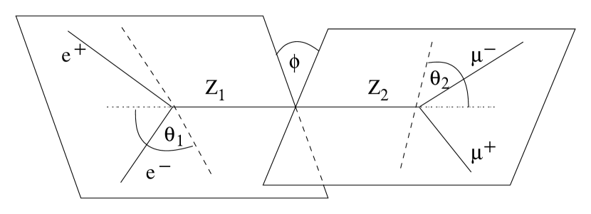
Figure 1: The decay plane angle $\phi$ is measured between the two planes defined by the leptons from the decay of the two Z bosons in the rest frame of the Higgs, using the charge of the leptons to fix the orientation of the planes. The dashed lines represent the direction of motion of the leptons in the rest frame of the Z Boson from which they originate. The angles $\theta_{1}$ and $\theta_{2}$ are measured between the negatively charged leptons and the direction of motion of the corresponding Z in the Higgs boson rest frame. $\phi$=0 correspond to $p_{e^{+}}\times p_{e^{-}}$ and $p_{\mu^{+}}\times p_{\mu^{-}}$ being parallel. $\phi$=$\pi$ correspond to $p_{e^{+}}\times p_{e^{-}}$ and $p_{\mu^{+}}\times p_{\mu^{-}}$ being antiparallel.

We study essentially two distributions. One is the distribution of the cosine of the polar angle, $\cos\theta$, of the decay leptons relative to the $Z$ boson. Because the heavy Higgs decays mainly into longitudinally polarised vector bosons the cross section $d\sigma/d\cos\theta$ should show a maximum around $\cos(\theta$)=0. The other is the distribution of the angle $\phi$ between the decay planes of the two $Z$ bosons in the rest frame of the Higgs boson. This distribution depends on the details of the Higgs decay mechanism. Within the Standard Model, a behaviour roughly like $1+\beta~{}\cos 2\phi$ is expected. This last distribution is flattened in the decay chain $H\rightarrow ZZ\rightarrow 4l$, because of the small vector coupling of the leptons, in contrast to the decay of the Higgs Boson into W’s or decay of the Z into quarks. Also, cuts can significantly affect the correlations. Therefore one needs a precise measurement of the momenta of the outgoing leptons. The Atlas-detector should be well-suited to measure these distributions, since the muon and electron reconstruction is very precise over a large solid angle. A detector Monte-Carlo is however needed in order to determine whether the angular distributions can be measured sufficiently well in order to determine the quantum numbers of the Higgs particle.

The present paper is organized as follows. In Chapter 2 the generator is described, in Chapter 3 detector simulation and reconstruction are given. In Chapter 4 we define quantities that can be used to characterize the different distributions. In Chapter 5 we present the results, concluding that the quantum numbers of the Higgs particle can indeed be determined. In the appendix we give formulae for the complete differential and integrated distributions for the decay of the resonance assuming arbitrary couplings computed in tree level and narrow width approximation.

2 The Generators

In order to distinguish between different spins J=0,1 and/or CP-eigenvalues $\gamma_{CP}=-1,+1$ one needs to study four different distributions: that resulting from the decay of the Standard Model Higgs boson, and the three distributions that would result from hypothetical particles with spin and CP-eigenvalue combinations (0, 1), (1, 1), (1, -1).

The feasibility of using angular correlations in the decay of the Z bosons in order to distinguish between these particles has been evaluated using two different Monte-Carlo generators. One was written for the Standard Model Higgs ($gg\rightarrow H\rightarrow ZZ\rightarrow 4l$) and the irreducible ZZ-background.[14] The latter includes contributions from both gluons and quarks to the ZZ production ( $gg\rightarrow ZZ\rightarrow 4l$ and $q\bar{q}\rightarrow ZZ\rightarrow 4l$) , whereas all Higgs production mechanisms other than the gluon fusion are neglected. This generator keeps all polarisations of the Z-boson for the quark initiated as well as for the gluon initiated processes. This allows for an analysis of the angular distributions of the leptons. The gluonic production of Z-boson pairs is only about 30% of the total background. However, one should not ignore its contribution, since it has different angular distributions from the other backgrounds and its presence can affect measured correlations. The programme contains no K-factors, therefore our conclusions regarding the feasibility of the determination of Higgs quantum numbers are conservative. Indeed, K-factors are expected to be larger for gluon-induced processes (such as the signal) than for quark-induced processes (70% of the background). Since the narrow width approximation is used, the results are only valid for Higgs masses above the ZZ threshold.

For the alternative particles, a new generator was written based on an article by C. A. Nelson and J. R. Dell’ Aquilla [13]. The programmes for the production of background, the Standard Model Higgs and all alternative particles use Cteq4M structure functions [16] and hdecay [17] for branching-ratio and width of the Higgs, and all use the narrow width approximation. The background as well as all cross sections for the four simulations are taken from the first generator. Thus, all cases show identical distributions of invariant mass of the Z-pairs and transverse momentum $P_{T}$ of Z-bosons and leptons and have the same width and cross sections. The only difference lies in the angular distributions of the leptons. For the alternative particles no special assumption concerning the coupling has to be made; only CP-invariance is assumed. It is worth mentioning that the angular correlations are completely independent of the production mechanism.

3 Detector Simulation and Reconstruction

The detector response is simulated using ATLFast [18], a software-package for particle level simulation of the Atlas detector. It is used for fast event-simulation including the most crucial detector aspects. Starting from a list of particles in the event, it provides a list of reconstructed jets, isolated leptons and photons and expected missing transverse energy. It applies momentum- and energy- smearing to all reconstructed particles. The values of the detector-dependent parameters are chosen to match the expected performance that was evaluated mostly by full simulations using Geant3[19].

The event selection is modeled exactly after the event selection in the Atlas-Physics-TDR [20]. Four leptons (electrons or muons) are required in the pseudorapidity range $|\eta|=|\ln\tan(\frac{\theta_{Beam}}{2})|\,<\,2.5$ ($\theta_{Beam}$ being the angle to the beam axis). Two of the leptons are required to have transverse momenta greater than 20 GeV/c and the two other leptons must have transverse momenta greater than 7 GeV/c each. A lepton identification efficiency of 90% per lepton was assumed. Two Z bosons are reconstructed by choosing lepton-pairs of matching flavour and opposite sign. If the flavours of all four leptons are equal, the combination is chosen, which minimizes the sum of the squared deviation of the invariant mass of the pairs with opposite sign from the Z mass (i.e. choose combination ab/cd that minimizes (m${}_{a^{+}b^{-}}$-m_Z)² + (m${}_{c^{+}d^{-}}$-m_Z)²). The reconstructed invariant mass of the two reconstructed Z bosons has to lie within two times the width of the reconstructed mass peak of the Higgs resonance around the centre of the peak. For high Higgs masses ($m_{H}>$ 300 GeV/c²) this is only little more than two times the decay width, while for smaller masses the experimental resolution dominates.

Throughout this paper, we use the term signal for distributions where the background has been statistically subtracted. The only background considered is the Z pair production. Other possible backgrounds like top pair production or Zbb are negligible for masses of the Higgs boson above 200 GeV/c². Systematic uncertainties due to the simulation of the background could be studied by comparing distributions from the sidebins of the Higgs signal with the results of the generator. A proper treatment of the background is very important, since the angular distributions of the background itself and correlations introduced by detector effects have a large impact on the shape of the distributions discussed. These effects are detailed below.

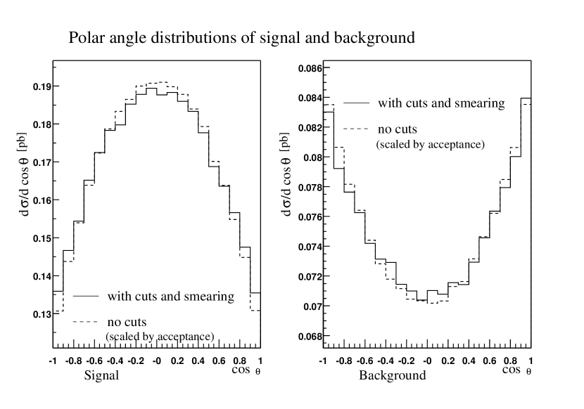
Figure 2: Distribution of the polar angle $\cos(\theta)$ for the background only (right) and the signal (left). The Higgs mass is 200 GeV/c².

For high invariant masses, the Z bosons from the background processes are mainly transversely polarised leading to a polar angle distribution of the form $\frac{d\sigma}{d\cos\theta}\sim 1+\cos^{2}\theta$. This distribution flattens the $\sin^{2}\theta$ distribution expected for the Higgs decay. Figure 2 shows the polar angle distributions of the signal (left) and the background (right). The dashed line shows the shape of the distribution expected when no cuts are applied and the detector response is not taken into account. It has just been scaled by the overall acceptance of the cuts, so that the shape can be compared. The expected distribution with all cuts and smearing applied is drawn as a solid line. Figures 2 and 3 are produced assuming a Higgs mass of 200 GeV/c² and Z decaying to muons only. For the decay ZZ $\rightarrow$ e⁺e^-e⁺e^- or ZZ $\rightarrow$ $\mu^{+}\mu^{-}$e⁺e^- the graphs look similar. The smearing effects are largely independent of the Higgs mass.

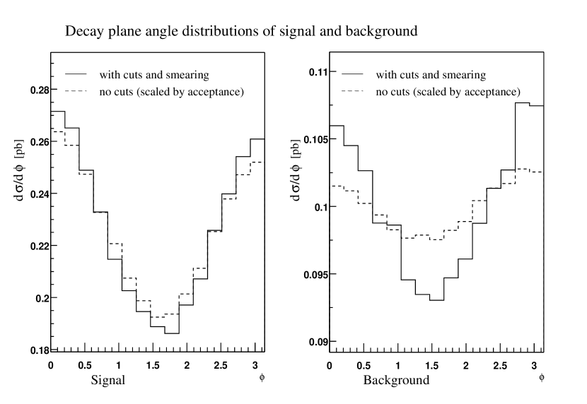
Figure 3: Distribution of the decay plane angle $\phi$ for the background only (right) and the signal (left). The Higgs mass is 200 GeV/c². The distribution without cuts is scaled by the expected acceptance, so that the shape can be directly compared.

The effect of the detector acceptance and isolation cuts on the decay plane angle distribution is shown in Figure 3. Again, the distribution of the signal is shown left and the background right. The dashed histogrammes are scaled to have the same integral as the solid histogrammes, and zero is suppresssed in order to facilitate the comparison of the shape. The definition of the line styles are the same as above. For the decay plane angle, the background shows an almost flat distribution before applying selection cuts. But a minor correlation is introduced by detector effects. This has been simulated and taken into account for the analysis of decay plane angle distributions. In conclusion, the isolation cuts lead to a small distortion of the angular distributions as discussed in [14], but these effects are almost negligible for the Atlas detector. The cut on $|\eta|$ enhances the decay plane correlation a little, but the smearing and the $P_{T}$ requirements reduce this effect. Altogether, there is a small enhancement of the correlation of almost the same amount for all four particles.

A further cut on the transverse momentum of the Z bosons $P_{T}^{max}(Z_{1},Z_{2})>m_{H}\,/\,3$ is known to additionally reduce the background, but it also affects the correlation. Since an optimisation of the signal-to-background ratio is not crucial to this analysis, this cut has not been applied, rendering the analysis less dependent on the details of the production mechanism like initial $P_{T}$ of the Higgs boson.

4 Parametrisation of Decay Angle Distributions

The differential cross sections for the different models can be computed directly or can be derived from the formulae given in [13]. The explicit distributions are given in the appendix. From the article [13] we quote the simple distributions of the alternative particles. Table 1 shows the distribution of the polar angle $\theta$. $\theta_{1}$ and $\theta_{2}$ are the polar angles of the leptons originating from the Z Bosons $Z_{1}$ and $Z_{2}$ respectively. In Table 2, the distribution of the decay plane angle $\phi$ is shown where the polar angle $\theta$ is integrated over different ranges. F11 gives the distribution for $0\leq\theta_{1,2}\leq\pi/2$, F22 for $\pi/2\leq\theta_{1,2}\leq\pi$, F12 for $0\leq\theta_{1}\leq\pi/2$ and $\pi/2\leq\theta_{2}\leq\pi$, and F21 for $\pi/2\leq\theta_{1}\leq\pi$ and $0\leq\theta_{2}\leq\pi/2$. $\cal R$, $\cal U$, $\cal T$ and $\cal W$ are the parameters that characterise the decay density matrix. For the decay modes used in this analysis, they amount to the following values: $\cal R$ = $\cal U$ = -1/2, $\cal T$ = $\cal W$ = $-\frac{2r}{1+r^{2}}$. r is the ratio of the axial vector to vector coupling which for the muons amounts to r = (1 - 4 $\sin^{2}\theta_{W})^{-1}$. We used $\sin^{2}\theta_{W}$ = 0.23.

Spin	$\gamma_{CP}$
0	-1	1 - $\cal R$$P_{2}(\cos\theta_{1})$ - $\cal U$$P_{2}(\cos\theta_{2})$ + $\cal R\cal U$$P_{2}(\cos\theta_{1})P_{2}(\cos\theta_{2})$ +
		$\frac{9}{4}$$\cal T$$\cal W$$P_{1}(\cos\theta_{1})P_{1}(\cos\theta_{2})$
1	+1	1 + $\frac{1}{2}$ $\cal R$$P_{2}(\cos\theta_{1})$ + $\frac{1}{2}$ $\cal U$ $P_{2}(\cos\theta_{2})$ -2 $\cal R\cal U$ $P_{2}(\cos\theta_{1})P_{2}(\cos\theta_{2})$
1	-1	1 + $\frac{1}{2}$ $\cal R$$P_{2}(\cos\theta_{1})$ + $\frac{1}{2}$ $\cal U$ $P_{2}(\cos\theta_{2})$ -2 $\cal R\cal U$ $P_{2}(\cos\theta_{1})P_{2}(\cos\theta_{2})$

Table 1: Distribution of the polar angle $\theta$. $P_{i}$ are the Legendre Polynomials. See the text for definitions.

Spin=0 $\gamma_{CP}$=-1
F11 + F22	$1+\frac{9}{16}\cal{T}\cal{W}-\cal{R}\cal{U}$$\cos(2\phi)$
F12 + F21	$1-\frac{9}{16}\cal{T}\cal{W}-\cal{R}\cal{U}$$\cos(2\phi)$
Spin=1 $\gamma_{CP}$=+1
F11 + F22	$1+(-\frac{1}{2}$$\cal R\cal U$$+\frac{1}{2}$$\cal T\cal W$$(\frac{3\pi}{8})^{2})\cos(\phi)$
F12 + F21	$1+(+\frac{1}{2}$$\cal R\cal U$$+\frac{1}{2}$$\cal T\cal W$$(\frac{3\pi}{8})^{2})\cos(\phi)$
Spin=1 $\gamma_{CP}$=-1
F11 + F22	$1+(+\frac{1}{2}$$\cal R\cal U$$-\frac{1}{2}$$\cal T\cal W$$(\frac{3\pi}{8})^{2})\cos(\phi)$
F12 + F21	$1+(-\frac{1}{2}$$\cal R\cal U$$-\frac{1}{2}$$\cal T\cal W$$(\frac{3\pi}{8})^{2})\cos(\phi)$

Table 2: Distribution of the decay plane angle $\phi$. F11 gives the distribution for $0\leq\theta_{1,2}\leq\pi/2$, F22 for $\pi/2\leq\theta_{1,2}\leq\pi$, F12 for $0\leq\theta_{1}\leq\pi/2$ and $\pi/2\leq\theta_{2}\leq\pi$ F21 for $\pi/2\leq\theta_{1}\leq\pi$ and $0\leq\theta_{2}\leq\pi/2$. $\cal R$ = $\cal U$ = -1/2 , $\cal T$ = $\cal W$ = $-\frac{2r}{1+r^{2}}$, r = (1 - 4 $\sin^{2}\theta_{W})^{-1}$.

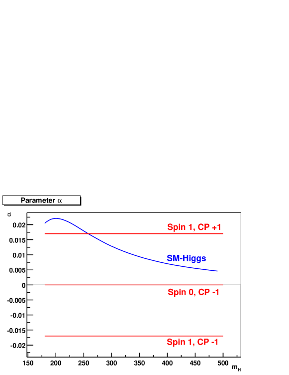
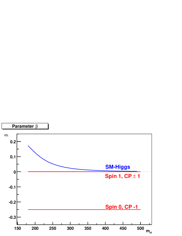
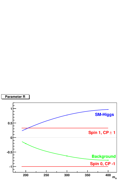
Figure 4: The variation of the three parameters $\alpha$, $\beta$ and $R$ (top to bottom) with the Higgs mass.

The plane-correlation can be parametrised as

$$F(\phi)=1+\alpha\cdot\cos(\phi)+\beta\cdot\cos(2\phi)$$ (1)

In all four cases discussed here, there is no $\sin(\phi)$ or $\sin(2\phi)$ contribution. For the Standard Model Higgs, $\alpha$ and $\beta$ depend on the Higgs mass while they are constant over the whole mass range in the other cases.

The polar angle distribution can be described by

$$G(\theta)=T\cdot(1+\cos^{2}(\theta))+L\cdot\sin^{2}(\theta)$$ (2)

reflecting the longitudinal or transverse polarisations of the Z boson. We define the ratio

$$R:=\frac{L-T}{L+T}$$ (3)

of transversal and longitudinal polarisation.
The dependence of the parameters $\alpha$, $\beta$ and $R$ on the Higgs mass is shown in Figure 4. The pseudoscalar shows the largest deviation from the SM Higgs. It would have $\beta=-0.25$ and $R=-1$ whereas the scalar always has $\beta>0$ and $R>0$. The vector and the axialvector can be excluded through the parameter $R$ for most of the mass range, but for Higgs masses around 200 GeV/c² the main difference lies in the value of $\beta$ which is zero for $J=1$ and $\gamma_{CP}=\pm 1$ and about 0.1 for the scalar. The value for $\alpha$ can only discriminate between the scalar and the axialvector but the difference is very small.

5 Background Estimation

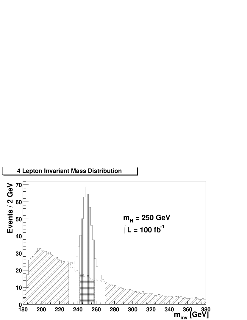
Figure 5: The invariant mass distribution of a 250 GeV/c² Higgs boson and the ZZ Background. The vertically hatched region is the signal region used in the analysis. The diagonally hatched regions are the sidebands used to determine the expected number of background events (hatched horizontally) inside the signal region. The dotted line indicates the shape of the background in the transition region between the sidebands and signal which is not used at all.

Figure 6: The parameter $R$ (defined in (3)) as obtained by a fit to different mass regions of the background only (solid line) and by a fit to the same mass regions to signal plus background distributions (points with errorbars). The horizontal errorbars indicate the regions from which the distributions where taken.

The subtraction of the angular distributions of the background is necessary to obtain and analize the angular distributions of the signal alone. This bears a risk of introducing systematic errors. Thus, the background distributions as produced by Monte-Carlo-Generators have to be checked against the data. In this chapter we will estimate the effects and possible systematic errors introduced by the subtraction.

First, the absolute number of background events has to be estimated. This can be done by comparing the sidebands of the signal to a simulated distribution of the background only. This procedure is illustrated in Figure 5. In order to obtain the number of expected events the number of simulated events in the signal region N${}^{MC}_{signal}$ is scaled by the number of events in the sidebands N${}^{Data}_{side}$ divided by the number of simulated events in the sidebands N${}^{MC}_{side}$. The error from this calculation is $\sigma_{\rm N}$ = $\sqrt{N^{Data}_{side}}\cdot\frac{N^{MC}_{signal}}{N^{MC}_{side}}$. In the case of a 250 GeV/c² Higgs boson the estimated number of background events is N=130 with a systematic error of $\sigma_{\rm N{\rm syst}}$ = 4.1 which is well below the statistical error of $\sigma_{\rm N{\rm stat}}$ = 11.4.

Checking of the shape of the background distribution can be done by using bins below and above the signal region, too. This is demonstrated in Figure 6. It shows the parameter $R$ derived from a fit described in chapter 4 to the background distribution only (black line) and the background plus signal (points with errorbars). For most of the fitted values a bin width of 20 GeV/c² was used, except for the last bin where 100 GeV/c² were used to compensate for the fact that there are less events for higher invariant masses. From the expected errors one finds that the parameter $R$ for the background can be estimated with a precision of about $\sigma_{\rm R}$ = 0.08. This might not seem too good, but the effect of using a slightly wrong background distribution is not so large. To demonstrate this, a fit to the angular distribution of the angle $\theta$ was performed, where a wrong background distribution was subtracted from the signal-plus-background distribution as obtained from the generator. The parameter R_sub of the subtracted distribution was changed to values higher and lower than the value of R_MC of the generated distributions. In Table 3, the difference $\Delta$R = R_MC - R_sub and the value of R_signal obtained from the fit to the signal distribution produced by subtracting the wrong background distribution are shown.

$\Delta$R	-0.2	-0.1	0.0	0.1	0.2
Rsignal	0.747	0.758	0.770	0.782	0.796

Table 3: The measured Parameter $R$ for five different distributions that have been used to subtract the expected background distribution. $\Delta$R is the difference between the value of $R$ from the background as produced by the Monte Carlo and the value of $R$ of the subtracted distribution.

The shift of the parameter is thus expected to be less than $\pm$0.01. Again, this is very small compared to the statistical error of $\Delta$R_stat = 0.053. This error is not considered in the rest of the analysis. Furthermore, the effects will be even smaller when considering K-factors. Any K greater than 1 will give better conditions to check the background distributions. And, since the K-factor of the gluonic Higgs production is higher than the K-factor of the main ZZ production process by quark antiquark pairs, the signal to background ratio will be even higher than predicted here.

6 Results

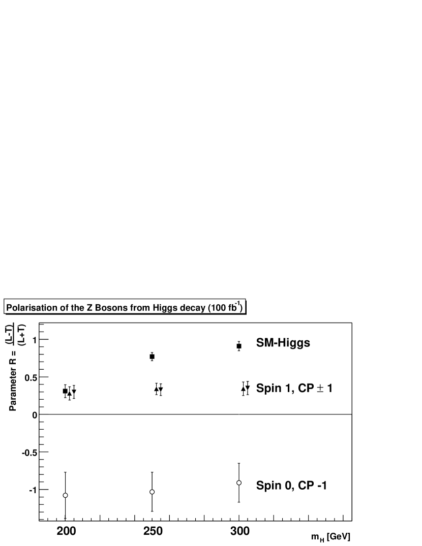
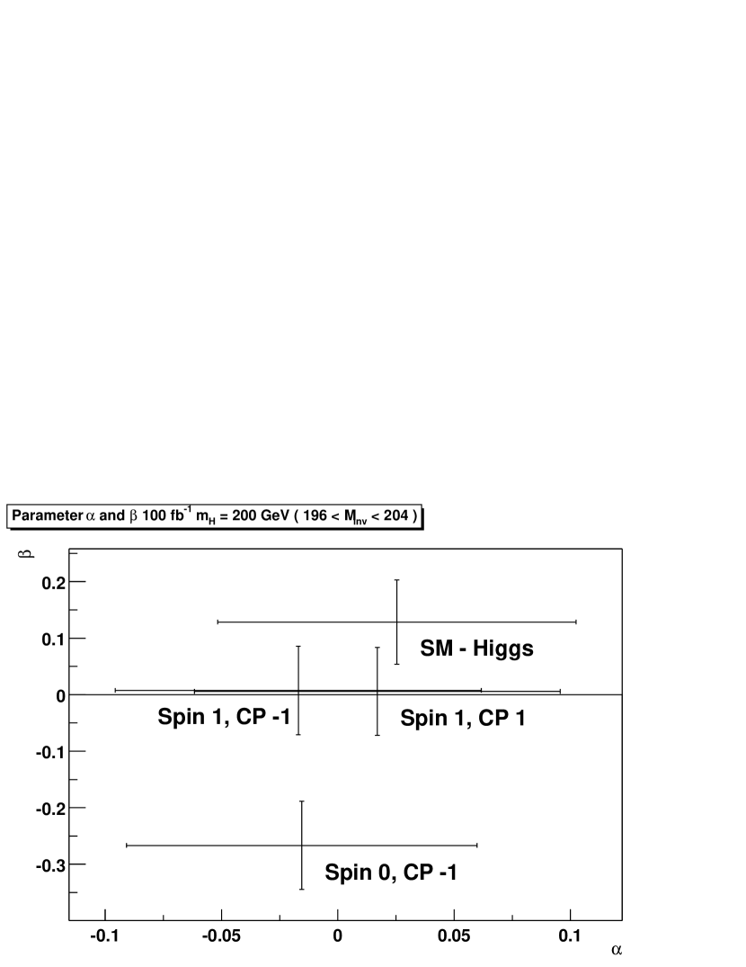
Figure 7: The parameter $R$ for different Higgs massses (top) and $\alpha$ and $\beta$ (bottom) for $m_{H}$ = 200 GeV/c² using 100 fb^-1. The error scales with the integrated luminosity as expected.

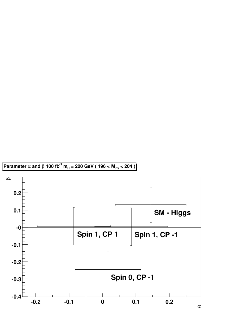
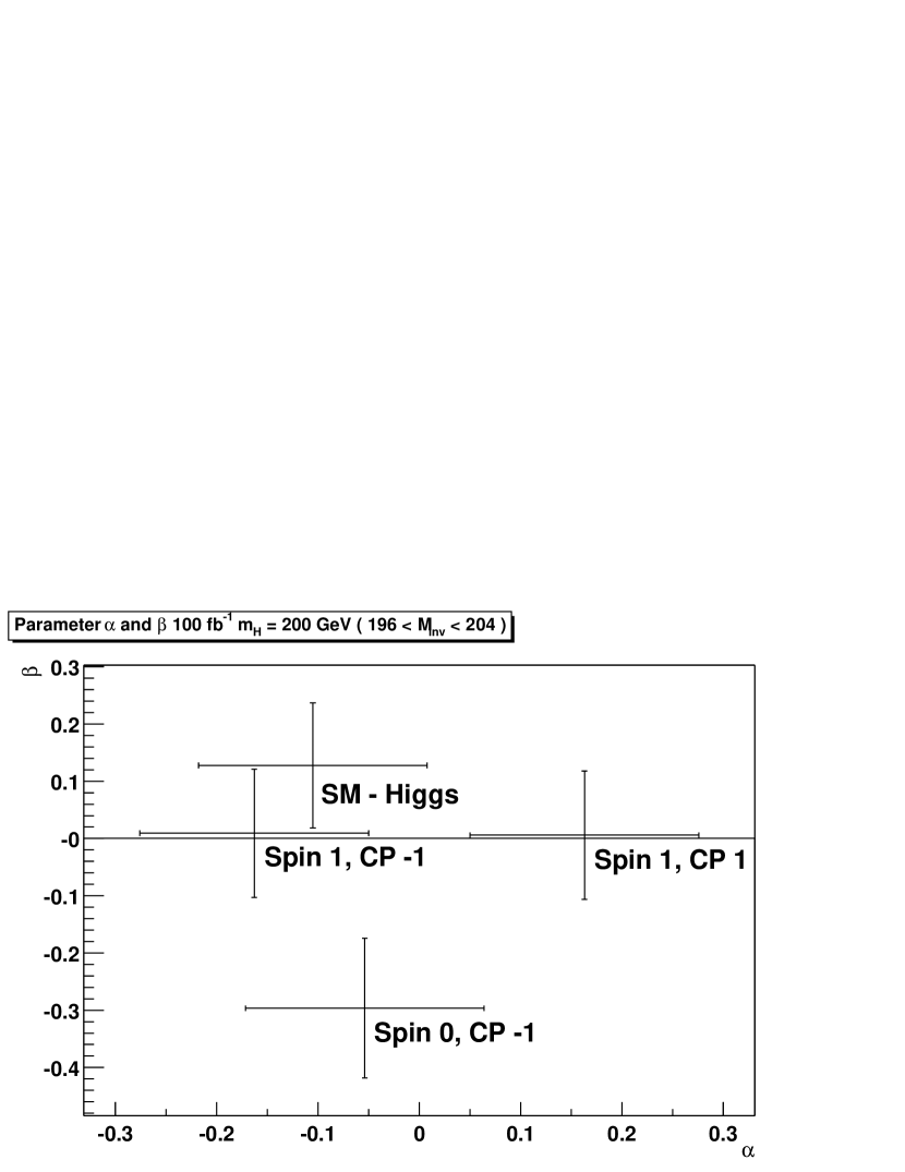
Figure 8: The parameter $\alpha$ depends on the signs of the $\cos(\theta)$ of the two Z bosons. The events where the signs are equal are used for the upper plot, those where the signs are different are used for the lower plot.

In Chapter 4, the exact results for the signal were given. However, in practice one needs a procedure to separate signal from background, which will lead to uncertainties in the distributions. The expected errors have been calculated by generating a large number of events and scaling the distributions to the expected number of events, since the expected values of the parameters follow a Gaussian distribution. The background was statistically subtracted after applying the same cuts to it as were applied to the signal. The error reflects the statistical error from the number of the signal events, the statistical error from the number of background events subtracted and the error made by the estimation of the number of background events as described in Chapter 5. No error from a possibly different angular distribution of background events has been taken into acount, but we have shown that the effect is small. Then the parametrisations for $\phi$ and $\theta$ as described above were fitted to the distributions. Signal and background are summed over muons and electrons.

Figure 7 (top) shows the expected values and errors for the parameter R, using an integrated luminosity of 100 fb^-1. It is clearly visible that for masses above 250 GeV/c² the measurement of this parameter allows the various hypotheses considered here for the spin and CP-state of the “Higgs Boson” to be unambiguously separated.

For a Higgs mass of 200 GeV/$c^{2}$ only the pseudoscalar is excluded. Figure 7 (bottom) shows the expected values and errors for $\alpha$ and $\beta$ for a 200 GeV/c² Higgs and an integrated luminosity of 100 fb^-1.

The parameter $\alpha$ can be used to distinguish between a spin 1 and the SM Higgs particle, but its use is statistically limited. The same applies to the parameter $\beta$. Measuring $\beta$, which is zero for spin 1 and $>$ 0 in the SM case, can contribute only very little to the spin measurement even if $m_{H}$ is in the range where $\beta$, in the SM case, is close to its maximum value. Nevertheless, $\beta$ can be useful to rule out a CP odd spin 0 particle.

The values of $\alpha$ get more widely separated when the correlation between the sign of $\cos(\theta)$ for the two Z Bosons and $\phi$ is exploited. In Figure 8, we plot the parameters separately for $sign(\cos\theta_{1})=sign(\cos\theta_{2})$ (F11 + F22 in Table 2) and $sign(\cos\theta_{1})=-sign(\cos\theta_{2})$ (F12 + F21 in Table 2). As can be seen, the difference in $\alpha$ becomes bigger for $J=1$ and $\gamma_{CP}=+1$. For higher masses $\alpha$ and $\beta$ of the SM Higgs approach 0; thus only $\alpha$ can be used to measure the spin. But the measurement of R compensates this.

Figure 9 shows the significance, i. e. the difference of the expected values divided by the expected error of the SM Higgs. We add up the significance for $\alpha$ and $\beta$ exploiting the $\cos(\theta)$ - $\phi$ correlation and plot the significance from the polar angle measurement separately. For higher Higgs masses the decay plane angle correlation contributes almost nothing, but the polarisation leads to a good measurement of the parameters spin and CP-eigenvalue. For full luminosity (300 fb^-1) the significance can simply be multiplied by $\sqrt{3}$. This is especially interesting for a Higgs mass of 200 GeV/c². The Spin 1, CP even hypothesis can then be ruled out with a significance of 6.4$\sigma$, while for the Spin 1, CP odd case the significance is still only 3.9$\sigma$.

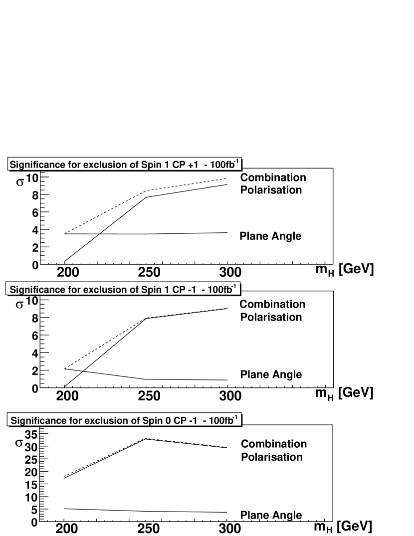
Figure 9: The overall significance for the exclusion of the non standard spin and CP-eigenvalue. The significance from the polar angle measurement and the decay-plane-correlation are plotted separately.

In conclusion, for Higgs masses larger than about 230 GeV/c² a Spin 1 hypothesis can be clearly ruled out already with 100 fb^-1. For m_H around 200 GeV/c² the distinction is less clear, and one will need the full integrated luminosity of the LHC. A spin-CP hypothesis of 0- can be ruled out with less than 100 fb${}^{-}1$ for the whole mass range above and around 200 GeV/c².

Appendix A Formulae for differential angular distributions

The most general coupling of a (pseudo) scalar Higgs boson to two on-shell Z-bosons is of the following form:

$${\cal L}_{scalar}=\mathbf{X}\delta_{\mu\nu}+\mathbf{Y}k_{\mu}k_{\nu}/M_{h}^{2}+i\mathbf{P}\epsilon_{\mu\nu p_{Z}q_{Z}}/M_{h}^{2}$$ (4)

Here the momentum of the first Z-boson is $p_{Z}^{\mu}$, that of the second Z-boson is $q_{Z}^{\nu}$. The momentum of the Higgs boson is $k$ and $\epsilon_{\mu\nu\rho\sigma}$ is the total antisymmetric tensor with $\epsilon_{1234}=i$. Within the Standard Model one has $\mathbf{X}=1$, $\mathbf{Y}=\mathbf{P}=0$. For a pure pseudoscalar particle one has $\mathbf{P}\not=0,\mathbf{X}=\mathbf{Y}=0$. If both $\mathbf{P}$ and one of the other interactions are present, one cannot assign a definite parity to the Higgs boson.

The same formula for a (pseudo) vector with momentum $k_{\rho}$ reads:

$${\cal L}_{vector}=\mathbf{X}(\delta_{\rho\mu}p_{Z}^{\nu}+\delta_{\rho\nu}q_{Z}^{\mu})+\mathbf{P}(i\epsilon_{\mu\nu\rho p_{Z}}-i\epsilon_{\mu\nu\rho q_{Z}})$$ (5)

It is to be noted that the coupling to the vector field actually contains only two parameters and is therefore simpler than to the scalar.

In the following we give the angular dependence of the triple differential cross section for the case of a scalar or vector Higgs decaying into two on-shell Z bosons which subsequently decay into two lepton pairs. The meaning of the angles $\theta_{1},\theta_{2}$ and $\phi$ is explained in Figure 1. $p$ is the absolute value of the momentum of the Z boson, $p^{2}=(\frac{1}{2}M_{h})^{2}-M_{Z}^{2}$. In the following we use the definitions $x=\frac{M_{h}}{M_{Z}}$ and $y=\frac{p}{M_{Z}}$. $c_{v}$ and $c_{a}$ are the vector and axial vector couplings: $c_{v}=t_{3}-2q\sin(\theta_{W})$, $c_{a}=t_{3}$, where $t_{3}$ is the weak isospin, $q$ the charge of the fermion and $\theta_{W}$ the Weinberg angle. For our case, the values of $c_{v}$ and $c_{a}$ are $c_{v}$ = -0.0379 and $c_{a}$ = -0.5014.

A.1 The general case

Scalar Higgs

$$\begin{split}&\frac{d\sigma}{d\phi d\cos\theta_{1}d\cos\theta_{2}}\sim\,\\ &-8{\mathbf{X}}{\mathbf{Y}}c_{a}^{2}c_{v}^{2}x^{2}(x^{2}-4)\cos\phi\sin\theta_{1}\sin\theta_{2}\\ &-{\mathbf{X}}{\mathbf{Y}}(c_{v}^{2}+c_{a}^{2})^{2}x^{2}(x^{2}-4)(2\cos\phi\sin\theta_{1}\sin\theta_{2}\cos\theta_{1}\cos\theta_{2}+(x^{2}-2)\sin^{2}\theta_{1}\sin^{2}\theta_{2})\\ &+16{\mathbf{X}}{\mathbf{P}}c_{a}^{2}c_{v}^{2}xy(x^{2}-2)\sin\phi\sin\theta_{1}\sin\theta_{2}\\ &+4{\mathbf{X}}{\mathbf{P}}(c_{v}^{2}+c_{a}^{2})^{2}xy\sin\phi(2\cos\phi\sin^{2}\theta_{1}\sin^{2}\theta_{2}+(x^{2}-2)\sin\theta_{1}\sin\theta_{2}\cos\theta_{1}\cos\theta_{2})\\ &+16{\mathbf{X}}^{2}c_{a}^{2}c_{v}^{2}x^{2}(2\cos\theta_{1}\cos\theta_{2}+(x^{2}-2)\cos\phi\sin\theta_{1}\sin\theta_{2})\\ &+{\mathbf{X}}^{2}(c_{v}^{2}+c_{a}^{2})^{2}x^{2}\{4(1+\cos^{2}\theta_{1}\cos^{2}\theta_{2}+\cos^{2}\phi\sin^{2}\theta_{1}\sin^{2}\theta_{2}\\ &+(x^{2}-2)\cos\phi\sin\theta_{1}\sin\theta_{2}\cos\theta_{1}\cos\theta_{2})+x^{2}(x^{2}-4)\sin^{2}\theta_{1}\sin^{2}\theta_{2}\}\\ &-8{\mathbf{P}}{\mathbf{Y}}c_{a}^{2}c_{v}^{2}xy(x^{2}-4)\sin\phi\sin\theta_{1}\sin\theta_{2}\\ &-2{\mathbf{P}}{\mathbf{Y}}(c_{v}^{2}+c_{a}^{2})^{2}xy(x^{2}-4)\sin\phi\sin\theta_{1}\sin\theta_{2}\cos\theta_{1}\cos\theta_{2}\\ &+1/4{\mathbf{Y}}^{2}(c_{v}^{2}+c_{a}^{2})^{2}x^{2}(x^{2}-4)^{2}\sin^{2}\theta_{1}\sin^{2}\theta_{2}\\ &+8{\mathbf{P}}^{2}c_{a}^{2}c_{v}^{2}(x^{2}-4)\cos\theta_{1}\cos\theta_{2}\\ &+{\mathbf{P}}^{2}(c_{v}^{2}+c_{a}^{2})^{2}(x^{2}-4)(1+\cos^{2}\theta_{1}\cos^{2}\theta_{2}-\cos^{2}\phi\sin^{2}\theta_{1}\sin^{2}\theta_{2})\\ \end{split}$$

Vector Higgs

$$\begin{split}&\frac{d\sigma}{d\phi d\cos\theta_{1}d\cos\theta_{2}}\sim\,\\ &-16{\mathbf{X}}{\mathbf{P}}c_{a}^{2}c_{v}^{2}xy\sin\phi\sin\theta_{1}\sin\theta_{2}\\ &+4{\mathbf{X}}{\mathbf{P}}(c_{v}^{2}+c_{a}^{2})^{2}xy\sin\phi\sin\theta_{1}\sin\theta_{2}\cos\theta_{1}\cos\theta_{2}\\ &+4{\mathbf{X}}^{2}c_{a}^{2}c_{v}^{2}x^{2}\cos\phi\sin\theta_{1}\sin\theta_{2}\\ &+{\mathbf{X}}^{2}(c_{v}^{2}+c_{a}^{2})^{2}x^{2}(1-\cos^{2}\theta_{1}\cos^{2}\theta_{2}-\cos\phi\sin\theta_{1}\sin\theta_{2}\cos\theta_{1}\cos\theta_{2})\\ &-4{\mathbf{P}}^{2}c_{a}^{2}c_{v}^{2}(x^{2}-4)\cos\phi\sin\theta_{1}\sin\theta_{2}\\ &+{\mathbf{P}}^{2}(c_{v}^{2}+c_{a}^{2})^{2}(x^{2}-4)(1-\cos^{2}\theta_{1}\cos^{2}\theta_{2}+\cos\phi\sin\theta_{1}\sin\theta_{2}\cos\theta_{1}\cos\theta_{2})\end{split}$$

A.2 The special cases

In this appendix we list the triple differential cross section for pure Higgs spin and CP states. In addition, we also give the differential cross sections, where some of the angular variables have been integrated over. F11, F12, F21, F22 refer to the different quadrants as defined in Chapter 4. The spin 0, CP even part only contains the pure SM contribution.

Spin 0, CP even

$$\begin{split}\frac{d\sigma}{d\phi d\cos\theta_{1}d\cos\theta_{2}}\sim\,&+16c_{a}^{2}c_{v}^{2}(2\cos\theta_{1}\cos\theta_{2}+(x^{2}-2)\cos\phi\sin\theta_{1}\sin\theta_{2})\\ &+(c_{v}^{2}+c_{a}^{2})^{2}\{4(1+\cos^{2}\theta_{1}\cos^{2}\theta_{2}+\cos^{2}\phi\sin^{2}\theta_{1}\sin^{2}\theta_{2}\\ &+(x^{2}-2)\cos\phi\sin\theta_{1}\sin\theta_{2}\cos\theta_{1}\cos\theta_{2})+x^{2}(x^{2}-4)\sin^{2}\theta_{1}\sin^{2}\theta_{2}\}\\ \frac{d\sigma}{d\cos\theta_{1}d\cos\theta_{2}}\sim\,&+32c_{a}^{2}c_{v}^{2}\cos\theta_{1}\cos\theta_{2}\\ &+(c_{v}^{2}+c_{a}^{2})^{2}\{4(1+\cos^{2}\theta_{1}\cos^{2}\theta_{2})+(x^{4}-4x^{2}+2)\sin^{2}\theta_{1}\sin^{2}\theta_{2}\}\\ \mbox{F11 = F22: }\frac{d\sigma}{d\phi}\sim\,&c_{a}^{2}c_{v}^{2}(8+\pi^{2}(x^{2}-2)\cos\phi)\\ &+4/9(c_{v}^{2}+c_{a}^{2})^{2}(x^{4}-4x^{2}+10+(x^{2}-2)\cos\phi+4\cos^{2}\phi)\\ \mbox{F12 = F21: }\frac{d\sigma}{d\phi}\sim\,&-c_{a}^{2}c_{v}^{2}(8-\pi^{2}(x^{2}-2)\cos\phi)\\ &+4/9(c_{v}^{2}+c_{a}^{2})^{2}(x^{4}-4x^{2}+10-(x^{2}-2)\cos\phi+4\cos^{2}\phi)\\ \end{split}$$

Spin 0, CP odd

$$\begin{split}\frac{d\sigma}{d\phi d\cos\theta_{1}d\cos\theta_{2}}\sim\,&+8c_{a}^{2}c_{v}^{2}\cos\theta_{1}\cos\theta_{2}\\ &+(c_{v}^{2}+c_{a}^{2})^{2}(1+\cos^{2}\theta_{1}\cos^{2}\theta_{2}-\cos^{2}\phi\sin^{2}\theta_{1}\sin^{2}\theta_{2})\\ \\ \frac{d\sigma}{d\cos\theta_{1}d\cos\theta_{2}}\sim\,&+16c_{a}^{2}c_{v}^{2}\cos\theta_{1}\cos\theta_{2}+(c_{v}^{2}+c_{a}^{2})^{2}(1+\cos^{2}\theta_{1})(1+\cos^{2}\theta_{2})\\ \\ \mbox{F11 = F22: }\frac{d\sigma}{d\phi}\sim\,&c_{a}^{2}c_{v}^{2}+1/9(c_{v}^{2}+c_{a}^{2})^{2}(5-2\cos^{2}\phi)\\ \\ \mbox{F12 = F21: }\frac{d\sigma}{d\phi}\sim\,&-c_{a}^{2}c_{v}^{2}+1/9(c_{v}^{2}+c_{a}^{2})^{2}(5-2\cos^{2}\phi)\end{split}$$

Spin 1, CP even

$$\begin{split}\frac{d\sigma}{d\phi d\cos\theta_{1}d\cos\theta_{2}}\sim\,&+4c_{a}^{2}c_{v}^{2}\cos\phi\sin\theta_{1}\sin\theta_{2}\\ &+(c_{v}^{2}+c_{a}^{2})^{2}(1-\cos^{2}\theta_{1}\cos^{2}\theta_{2}-\cos\phi\sin\theta_{1}\sin\theta_{2}\cos\theta_{1}\cos\theta_{2})\\ \\ \frac{d\sigma}{d\cos\theta_{1}d\cos\theta_{2}}\sim\,&1-\cos^{2}\theta_{1}\cos^{2}\theta_{2}\\ \\ \mbox{F11 = F22: }\frac{d\sigma}{d\phi}\sim\,&+c_{a}^{2}c_{v}^{2}\pi^{2}\cos\phi+1/9(c_{v}^{2}+c_{a}^{2})^{2}(32-4\cos\phi)\\ \\ \mbox{F12 = F21: }\frac{d\sigma}{d\phi}\sim\,&+c_{a}^{2}c_{v}^{2}\pi^{2}\cos\phi+1/9(c_{v}^{2}+c_{a}^{2})^{2}(32+4\cos\phi)\\ \end{split}$$

Spin 1, CP odd

$$\begin{split}\frac{d\sigma}{d\phi d\cos\theta_{1}d\cos\theta_{2}}\sim\,&-4c_{a}^{2}c_{v}^{2}\cos\phi\sin\theta_{1}\sin\theta_{2}\\ &+(c_{v}^{2}+c_{a}^{2})^{2}(1-\cos^{2}\theta_{1}\cos^{2}\theta_{2}+\cos\phi\sin\theta_{1}\sin\theta_{2}\cos\theta_{1}\cos\theta_{2})\\ \\ \frac{d\sigma}{d\cos\theta_{1}d\cos\theta_{2}}\sim\,&1-\cos^{2}\theta_{1}\cos^{2}\theta_{2}\\ \\ \mbox{F11 = F22: }\frac{d\sigma}{d\phi}\sim\,&-c_{a}^{2}c_{v}^{2}\pi^{2}\cos\phi+1/9(c_{v}^{2}+c_{a}^{2})^{2})(32+4\cos\phi)\\ \\ \mbox{F12 = F21: }\frac{d\sigma}{d\phi}\sim\,&-c_{a}^{2}c_{v}^{2}\pi^{2}\cos\phi+1/9(c_{v}^{2}+c_{a}^{2})^{2})(32-4\cos\phi)\\ \\ \end{split}$$

References

- [1] ALEPH, DELPHI, L3, OPAL and the Electroweak Working Group for Higgs Boson Searches, Phys. Lett. B565 (2003) 61.
- [2] The LEP Electroweak Working Group, LEP EWWG Home Page. URL: http://lepewwg.web.cern.ch/LEPEWWG (2003).
- [3] K. Moenig, Electroweak precision data and the Higgs mass: Workshop summary, hep-ph/0308133 (2003).
- [4] M. E. Peskin, Phys. Rev. D64 (2001) 093003.
- [5] For a short review of the Higgs search status at the LHC; F. Piccinini, contribution to ICHEP 2002, hep-ph/0209377 (2002).
- [6] D. Dominici, Riv. Nuovo Cim. 20, 11 (1997).
- [7] B. Kastening and J. J. van der Bij Phys. Rev. D60: 095003 (1999).
- [8] C. N. Yang Phys. Rev. 77, 242 (1950).
- [9] A recent review; C. Quigg, Acta Phys. Polon. B30, 2145 (1999).
- [10] A. Abbasabadi and W. W. Repko, Nucl. Phys. B292, (1987) 461 and Phys. Rev. D37, (1988) 2668.
- [11] M. J. Duncan, Phys. Lett. B179, (1986) 393.
- [12] M. J. Duncan, G. L. Kane and W. W. Repko, Phys. Rev. Lett. 55, (1985) 773 and Nucl. Phys. B272, (1986) 517.
-
[13]
J. R. Dell’Aquila and C. A. Nelson, Phys. Rev. D33,
(1986) 80;
C. A. Nelson, Phys. Rev. D37, (1988) 1220. - [14] T. Matsuura and J. J. van der Bij, Z. Phys. C51, 259 (1991).
- [15] S. Y. Choi, D. J. Miller, M. M. Muhlleitner, P. M. Zerwas. Phys. Lett. B553 (2003) 61.
- [16] H. L. Lai, J. Huston, S. Kuhlmann, F. Olness, J. Owens, D. Soper, W.K. Tung, H. Weerts. hep-ph/9606399. 1996
- [17] A. Djouadi, J. Kalinowski, M.Spira. Comput. Phys. Commun. 108 (1998) 56.
- [18] E. Richter-Was, D. Froidevaux, L. Pogglioli. ATL-PHYS-98-131. 1998
- [19] Atlas Detector and Physics Performance. Technical Design Report. Volume 1. CERN 1999
- [20] Atlas Detector and Physics Performance. Technical Design Report. Volume 2. CERN 1999