Abstract

Supersymmetric particles can be produced copiously at future colliders. From the high-precision data taken at $e^{+}e^{-}$ linear colliders, TESLA in particular, and combined with results from LHC, and CLIC later, the low-energy parameters of the supersymmetric model can be determined. Evolving the parameters from the low-energy scale to the high-scale by means of renormalization group techniques the fundamental supersymmetry parameters at the high scale, GUT or Planck, can be reconstructed to reveal the origin of supersymmetry breaking.

1 Introduction

Despite the lack of direct experimental evidence for supersymmetry (SUSY), the concept of symmetry between bosons and fermions has so many attractive features that the supersymmetric extension of the Standard Model is widely considered as a most natural scenario. It protects the electroweak scale from destabilizing divergences, leads to the unification of gauge couplings, accommodates a large top quark mass, provides a natural candidate for dark matter, and decouples from precision measurements. Exact supersymmetry is a fully predictive framework: to each known particle it predicts the existence of its superpartner which differs in the spin quantum number by 1/2, and fixes their couplings without introducing new parameters. Thus the Minimal Supersymmetric extension of the Standard Model (MSSM) encompasses spin 1/2 partners of the gauge and Higgs bosons, called gauginos and higgsinos, and spin 0 companions of leptons and quarks, called sleptons and squarks.

If realized in nature, supersymmetry (SUSY) must be a broken symmetry since until now none of the superpartners have been found. The construction of a viable mechanism of SUSY breaking, however, is a difficult issue. It is impossible to construct a realistic breaking scenario with the particle content of the MSSM [2]. Therefore the origin of SUSY breaking is usually assumed to take place in a “hidden sector” of particles which have no direct couplings to the MSSM particles and the supersymmetry breaking is “mediated” from the hidden to the visible sector. This opens up a variety of possible scenarios of SUSY breaking and its mediation, and in fact many models have been proposed: gravity-mediated, gauge-mediated, anomaly-mediated, gaugino-mediated etc. Each model is characterized by a few parameters (usually defined at a high scale) and leads to different phenomenological consequences.

With all the different SUSY models proposed in the past, the best is to keep an open mind and parameterize the breaking of SUSY by the most general explicit breaking terms in the Lagrangian. The structure of the breaking terms is constrained by the gauge symmetry and the requirement of stabilization against radiative corrections from higher scales. This leads to a set of soft-breaking terms [3], which include
(i) gaugino mass terms for bino $\tilde{B}$, wino $\tilde{W}^{j}$ $[j=$1–3] and gluino $\tilde{g}^{i}$ $[i=$1–8]

$${\textstyle\frac{1}{2}}M_{1}\,\overline{\tilde{B}}\,\tilde{B}\ +\ {\textstyle\frac{1}{2}}M_{2}\,\overline{\tilde{W}}^{i}\,\tilde{W}^{i}\ +\ {\textstyle\frac{1}{2}}M_{3}\,\overline{\tilde{g}}^{i}\,\tilde{g}^{i}\ ,$$ (1)

(ii) trilinear ($A^{i}$) and bilinear ($B$) scalar couplings (generation indices are understood)

$$A_{u}H_{2}\tilde{Q}\tilde{u}^{c}+A_{d}H_{1}\tilde{Q}\tilde{d}^{c}+A_{l}H_{1}\tilde{L}\tilde{l}^{c}-\mu BH_{1}H_{2}$$ (2)

(iii) and squark and slepton mass terms

$$m_{\tilde{Q}}^{2}[\tilde{u}^{*}_{L}\tilde{u}_{L}+\tilde{d}^{*}_{L}\tilde{d}_{L}]+m_{\tilde{u}}^{2}\tilde{u}^{*}_{R}\tilde{u}_{R}+m_{\tilde{d}}^{2}\tilde{d}^{*}_{R}\tilde{d}_{R}+\ \cdots$$ (3)

where the ellipses stand for the soft mass terms for sleptons and Higgs bosons (tilde denotes the superpartner). The above parameters can be complex with nontrivial CP violating phases [4]. The stability of quantum corrections implies that at least some of the superpartners should be relatively light, with masses around 1 TeV, and thus within the reach of present or next generation of high-energy colliders.

As a consequence of the most general soft-breaking terms, a large number of parameters is introduced. The unconstrained low-energy MSSM has some 100 parameters resulting in a rich spectroscopy of states and complex phenomenology of their interactions. One should realize, that the low-energy parameters are of two distinct categories. The first one includes all the gauge and Yukawa couplings and the higgsino mass parameter $\mu$. They are related by exact supersymmetry which is crucial for the cancellation of quadratic divergences. For example, at tree-level the $qqZ$, $\tilde{q}\tilde{q}Z$ gauge and $q\tilde{q}\tilde{Z}$ Yukawa couplings have to be equal. The relations among these parameters (with calculable radiative corrections) have to be confirmed experimentally; if not – the supersymmetry is excluded. The second category encompasses all soft-supersymmetry breaking parameters: higgsino, gaugino and sfermion masses and mixing, and the trilinear couplings.

If supersymmetry is detected at a future collider it will be a matter of days to discover all kinetically accessible supersymmetric particles. However, it will be an enormous task to investigate the masses, couplings and quantum numbers of the superpartners and many measurements and considerable ingenuity will be needed to reconstruct a complete low-energy theory. The experimental program to search for and explore SUSY at present and future colliders has to include the following points:
          (a) discover supersymmetric particles and measure their quantum numbers to prove
               that they are the superpartners of standard particles,
          (b) measure their masses, mixing angles and couplings,
          (c) determine the low-energy Lagrangian parameters,
          (d) verify the relations among them in order to distinguish between various SUSY
               breaking models.

It is important to realize that all low-energy SUSY parameters should be measured independently of any theoretical assumptions. In this respect the concept of a high-energy $e^{+}e^{-}$ linear collider [5] is of particular interest since it opens up a possibility of precision measurements of supersymmetric particle properties. An intense activity during last few years on $e^{+}e^{-}$ collider physics has convincingly demonstrated the advantages and benefits of such a machine and its complementarity to the Large Hadron Collider (LHC). Many studies have shown that the LHC can cover a mass range for SUSY particles up to $\sim$ 2 TeV, in particular for squarks and gluinos [6]. Early indication of SUSY can be provided by an excess in $M_{eff}=E^{T}_{miss}+p^{T}_{1}+p^{T}_{2}+\ldots$, an example is shown in Fig.1, where $E^{T}_{miss}$ is due to the stable lightest SUSY particles (LSP) escaping detection, and $p^{T}_{i}$ are transverse momenta of jets. Sparticles from squark and gluino decays can be accessed if the SUSY decays are distinctive. The problem however is that many different sparticles will be accessed at once with the heavier ones cascading into the lighter which will in turn cascade further leading to a complicated picture. Simulations for the extraction of parameters have been attempted for the LHC and demonstrated that some of them can be extracted with a good precision. Identifying particular decay channels and measuring the endpoints, for example in the dilepton invariant mass as shown in Fig.1, the mass differences of SUSY particles can be determined very precisely. If enough channels are identified and measured, the masses can be determined without any model assumptions. With a large amount of information available from the production of squarks and gluinos and their main decay products, theoretical interpretation can be possible in favorable models.

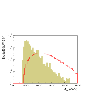
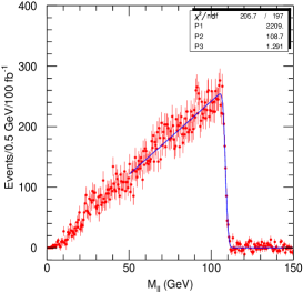
Figure 1: Left: Typical $M_{eff}$ spectrum. Right: The dilepton invariant mass distribution. From [6].

But if all proposed theoretical models of the SUSY breaking turn out to be wrong, the concurrent running of an $e^{+}e^{-}$ LC will be very much welcome. It will provide information complementary to that from the LHC. Thanks to
          $\diamond$ clean final state environment,
          $\diamond$ tunable energy,
          $\diamond$ polarized incoming beams,
          $\diamond$ and a possibility of additional modes: $e^{-}e^{-}$, $e\gamma$ and $\gamma\gamma$
precise determination of masses, couplings, quantum numbers, mixing angles and CP phases will be possible at $e^{+}e^{-}$ colliders. As I will illustrate with some examples below, this will allow us a model independent reconstruction of the low-energy SUSY parameters to be performed and, hopefully, connect the low-scale phenomenology with the high-scale physics [7].

2 Reconstruction of low-energy SUSY parameters

In contrast to many earlier analyzes, we will not elaborate on global fits but rather we will discuss attempts at “measuring” the fundamental Lagrangian parameters. Generically such attempts are performed in two steps [8]
          $A$: from the observed quantities: cross sections, asymmetries etc. determine the
               physical parameters: the masses, mixing and couplings of sparticles,
          $B$: from the physical parameters extract the Lagrangian parameters: $M_{i}$, $\mu$, $\tan\beta$,
               $A^{u}$, $m_{\tilde{Q}}$ etc.

To deal with so many parameters, a clear strategy is needed. An attractive possibility would be to
          $\diamond$ start with charginos which depend only on $M_{2}$, $\mu$, $\tan\beta$,
          $\diamond$ add neutralinos which depend in addition on $M_{1}$,
          $\diamond$ include sleptons which bring in $m_{\tilde{l}}$, $A_{l}$,
          $\diamond$ and finally squarks and gluinos to determine $m_{\tilde{q}}$, $A_{q}$ and $M_{3}$
to reconstruct at tree level the basic structure of SUSY Lagrangian. In reality it might be difficult to separate a specific sector (e.g. sleptons enter via t-channel in the chargino production processes), many production channels can simultaneously be open, and SUSY constitutes an important background to SUSY processes. In addition sizable loop corrections will mix all sectors. Precision measurements will require loop corrections to the masses and mixing angles, the finite decay width effects and loop corrections to the production and decay processes to be included for final global analyzes of all data. Some one-loop results are already available: for the current status we refer to [9].

2.1 The chargino sector

The mass matrix of the wino and charged higgsino, after the gauge symmetry breaking, is nondiagonal

$${\cal M}_{C}=\left(\begin{array}[]{cc}M_{2}&\sqrt{2}m_{W}\cos\beta\\ \sqrt{2}m_{W}\sin\beta&|\mu|{\rm e}^{i\Phi_{\mu}}\end{array}\right)\$$ (6)

It can be diagonalized by two unitary matrices acting on left- and right-chiral states

$$U_{L}=\left(\begin{array}[]{cc}c_{L}&s_{L}^{*}\\ -s_{L}&c_{L}\end{array}\right),\qquad U_{R}=\left(\begin{array}[]{cc}{\rm e}^{i\gamma_{1}}&0\\ 0&{\rm e}^{i\gamma_{2}}\end{array}\right)\left(\begin{array}[]{cc}c_{R}&s_{R}^{*}\\ -s_{R}&c_{R}\end{array}\right)$$ (13)

with $c_{L,R}=\cos\phi_{L,R}$, $s_{L,R}={\rm e}^{i\beta_{L,R}}\sin\phi_{L,R}$, which involve two mixing angles $\phi_{L,R}$ and three CP phases $\beta_{L,R}$ and $\gamma_{1}-\gamma_{2}$ The mass eigenstates, called charginos, are mixtures of wino and higgsino with the masses and mixing angles given by

$$m^{2}_{\tilde{\chi}^{\pm}_{1,2}}=\frac{1}{2}\left[M^{2}_{2}+|\mu|^{2}+2m^{2}_{W}\mp{\Delta_{C}}\right]$$ (14)

$$\cos 2\phi_{L,R}=-\left[M_{2}^{2}-|\mu|^{2}\mp 2m^{2}_{W}\cos 2\beta\right]/{\Delta_{C}}$$ (15)

where $\Delta_{C}=[(M^{2}_{2}-|\mu|^{2})^{2}+4m^{4}_{W}\cos^{2}2\beta+4m^{2}_{W}(M^{2}_{2}+|\mu|^{2})+8m^{2}_{W}M_{2}|\mu|\sin 2\beta\cos{\Phi_{\mu}}]^{1/2}$. Experimentally the chargino masses can be measured very precisely either by threshold scans or in continuum above the threshold [10]. Since the chargino production cross sections are simple binomials of $\cos 2\phi_{L,R}$, see Fig.2, the mixing angles can be determined in a model independent way using polarized electron beams [11, 12].

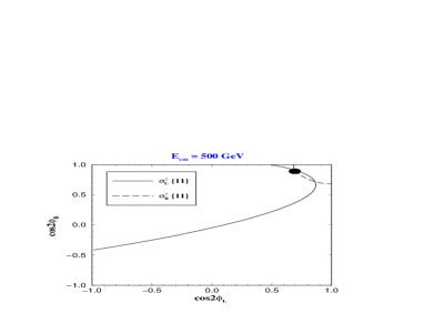
Figure 2: Contours of the light chargino production cross sections with polarized electron beams in the plane $[\cos 2\phi_{L},\cos 2\phi_{R}]$. From [12].

Based on this high-precision information, the fundamental SUSY parameters can be extracted in analytic form. Inverting eqs.(14,15) one finds to lowest order:

$$M_{2} = M_{W}[\Sigma-\Delta[\cos 2\phi_{R}+\cos 2\phi_{L}]]^{1/2}$$ (16)

$$\left|\mu\right| = M_{W}[\Sigma+\Delta[\cos 2\phi_{R}+\cos 2\phi_{L}]]^{1/2}$$ (17)

$$\cos\Phi_{\mu} = [\Delta^{2}-(M^{2}_{2}-\mu^{2})^{2}-4m^{2}_{W}(M^{2}_{2}+\mu^{2})$$ (18)

$$-4m^{4}_{W}\cos^{2}2\beta]/8m_{W}^{2}M_{2}|\mu|\sin 2\beta$$

$$\tan\beta = \left[\frac{1+\Delta(\cos 2\phi_{R}-\cos 2\phi_{L})}{1-\Delta(\cos 2\phi_{R}-\cos 2\phi_{L})}\right]^{1/2}$$ (19)

where $\Delta=\Delta_{C}/4M^{2}_{W}==(m^{2}_{\tilde{\chi}^{\pm}_{2}}-m^{2}_{\tilde{\chi}^{\pm}_{1}})/4M^{2}_{W}$ and $\Sigma=(m^{2}_{\tilde{\chi}^{\pm}_{2}}+m^{2}_{\tilde{\chi}^{\pm}_{1}})/2M^{2}_{W}-1$.

If both $m_{\tilde{\chi}^{\pm}_{1}}$ and $m_{\tilde{\chi}^{\pm}_{2}}$ can be measured, the fundamental parameters (16-19) can be extracted unambiguously. However, if $\tilde{\chi}^{\pm}_{2}$ happens to be beyond the kinematical reach at an early stage of the LC, it depends on the CP properties of the higgsino sector whether they can be determined or not in the light chargino system alone [12]

(i)  If the higgsino sector is CP invariant, $\cos\Phi_{\mu}=\pm 1$ can be exploited to determine $m_{\tilde{\chi}^{\pm}_{2}}$ up to at most a two–fold ambiguity. This ambiguity can be resolved if other observables can be measured, e.g. the mixed–pair $\tilde{\chi}^{0}_{1}\tilde{\chi}^{0}_{2}$ production cross sections.

(ii)  In a CP non–invariant theory the parameters in eqs.(16–19) remain dependent on the unknown heavy chargino mass $m_{\tilde{\chi}^{\pm}_{2}}$. Two trajectories in the plane $[\cos 2\phi_{L},\cos 2\phi_{R}]$ are generated (and consequently in the $\{M_{2},\mu;\tan\beta\}$ space), parametrized by $m_{\tilde{\chi}^{\pm}_{2}}$ and classified by the two possible signs of $\sin\Phi_{\mu}$. The analysis of the two light neutralino states $\tilde{\chi}^{0}_{1}$ and $\tilde{\chi}^{0}_{2}$ can be used to predict the heavy chargino mass $m_{\tilde{\chi}^{\pm}_{2}}$ in the MSSM. Therefore we will now discuss

2.2 The neutralino sector

The mass matrix of the $(\tilde{B},\tilde{W}^{3},\tilde{H}^{0}_{1},\tilde{H}^{0}_{2})$ is symmetric but nondiagonal

$$M_{N}=\left(\begin{array}[]{cccc}M_{1}&0&-m_{Z}c_{\beta}s_{W}&m_{Z}s_{\beta}s_{W}\\ 0&M_{2}&m_{Z}c_{\beta}c_{W}&-m_{Z}s_{\beta}c_{W}\\ -m_{Z}c_{\beta}s_{W}&m_{Z}c_{\beta}c_{W}&0&-\mu\\ m_{Z}s_{\beta}s_{W}&-m_{Z}s_{\beta}c_{W}&-\mu&0\end{array}\right)\$$ (24)

where $M_{1}=|M_{1}|\,\,{\rm e}^{i\Phi_{1}}$, $\mu=|\mu|\,\,{\rm e}^{i\Phi_{\mu}}$. The mass eigenstates, neutralinos, are obtained by the $4\times 4$ diagonalization matrix $N$, which is parameterized by 6 angles and 10 phases as

$$N = {\sf diag}\left\{{\rm e}^{i\alpha_{1}},\,{\rm e}^{i\alpha_{2}},\,{\rm e}^{i\alpha_{3}},\,{\rm e}^{i\alpha_{4}}\,\right\}{\sf R}_{34}\,{\sf R}_{24}\,{\sf R}_{14}\,{\sf R}_{23}\,{\sf R}_{13}\,{\sf R}_{12}$$ (25)

where ${\sf R}_{jk}$ are $4\times 4$ matrices describing 2-dim complex rotations in the {jk} plane (of the form analogous to $U_{L}$ in eq.(13) and defined in terms of ($cos\theta_{jk}$, $\sin\theta_{jk}\,{\rm e}^{i\delta_{jk}})$).

The CP is conserved in the neutralino sector if $\delta_{ij}=0$ and $\alpha_{i}=0$. The unitarity constraints can conveniently be formulated in terms of unitarity quadrangles built up by
          $\diamond$ the links $N_{ik}N^{*}_{jk}$ connecting two rows $i$ and $j$
          $\diamond$ the links $N_{ki}N^{*}_{kj}$ connecting two columns $i$ and $j$.
Unlike in the CKM or MNS cases of quark and lepton mixing, the orientation of all quadrangles is physical [12].

To resolve the light chargino case in the CP-violating scenario (ii), we note that each neutralino mass satisfies the characteristic equation

$$m_{\tilde{\chi}^{0}_{i}}^{8}-a\,m_{\tilde{\chi}^{0}_{i}}^{6}+b\,m_{\tilde{\chi}^{0}_{i}}^{4}-c\,m_{\tilde{\chi}^{0}_{i}}^{2}+d=0$$ (26)

where $a$, $b$, $c$ and $d$ are binomials of  $\Re{\rm e}{M_{1}}$ and  $\Im{\rm m}{M_{1}}$. Therefore the equation for each $m^{2}_{\tilde{\chi}^{0}_{i}}$ has the form

$$(\Re{\rm e}{M_{1}})^{2}+(\Im{\rm m}{M_{1}})^{2}+u_{i}\,\Re{\rm e}{M_{1}}+v_{i}\,\Im{\rm m}{M_{1}}=w_{i}$$ (27)

i.e. each neutralino mass defines a circle in the $\{\Re{\rm e}M_{1},\Im{\rm m}M_{1}\}$ plane. With two light neutralino masses two crossing points in the ($\Re{\rm e}{M_{1}}$, $\Im{\rm m}{M_{1}}$) plane are generated, as seen in the left panel of Fig.3.

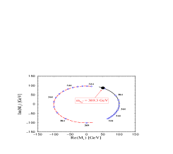
Figure 3: Left: Contour lines for two light neutralino masses in the ($\Re{\rm e}{M_{1}}$, $\Im{\rm m}{M_{1}}$) plane. Right: The migration with $m_{\tilde{\chi}^{\pm}_{2}}$ of two crossing points. From [12].

Since from the chargino sector $\{M_{2},\mu\;\tan\beta\}$ are parameterized by unknown $m_{\tilde{\chi}^{\pm}_{2}}$, the crossing points will migrate with $m_{\tilde{\chi}^{\pm}_{2}}$, right panel of Fig.3. One can use the measured cross section for $\tilde{\chi}^{0}_{1}\tilde{\chi}^{0}_{2}$ to select a unique solution for $M_{1}$ and predict the heavy chargino mass. If the LC runs concurrently with the LHC, the LHC experiments may be able to verify the predicted value of $m_{\tilde{\chi}^{\pm}_{2}}$.

If the machine energy is above the heavy charginos and neutralinos, one can
          $\diamond$ study the threshold behavior of non-diagonal neutralino pair production to check
             for a clear signal of nontrivial CP phases,
          $\diamond$ measure the normal neutralino polarization which provides a unique probe of
             $\alpha_{i}$ (Majorana) CP phases,
          $\diamond$ exploit the sum rules to verify the closure of the chargino and neutralino sectors,
          $\diamond$ analyze the SUSY relations between Yukawa and gauge couplings,
          $\diamond$ extract information on sleptons exchanged in the t-channels etc.
For more details, we refer to [13].

2.3 The sfermion sector

The sfermion mass matrix in the $(\tilde{f}_{L},\tilde{f}_{R})$ basis is given as

$$\left(\begin{array}[]{cc}{\ M^{2}_{\tilde{F_{L}}}}+m^{2}_{Z}\cos 2\beta(I_{f_{i}}-Q_{f}\sin^{2}\theta_{W})+m_{f}^{2}&m_{f}({\ A_{f}^{*}}-{\ \mu}(\cot\beta)^{2I_{f}})\\ m_{f}({\ A_{f}}-{\ \mu}^{*}(\cot\beta)^{2I_{f}})&{\ M^{2}_{\tilde{f_{R}}}}-m^{2}_{Z}Q_{f}\cos 2\beta\sin^{2}\theta_{W}+m_{f}^{2}\end{array}\right)\$$ (30)

where $M^{2}_{\tilde{F_{L}}}$, $M^{2}_{\tilde{f_{R}}}$ and $A_{f}$ are slepton soft SUSY breaking parameters. The mass eigenstates are defined

$$\left(\begin{array}[]{c}\tilde{f}_{1}\\ \tilde{f_{2}}\end{array}\right)=\left(\begin{array}[]{cc}{\rm e}^{i\alpha_{f}}\cos\theta_{f}&\sin\theta_{f}\\ -\sin\theta_{f}&{\rm e}^{-i\alpha_{f}}\cos\theta_{f}\end{array}\right)\left(\begin{array}[]{c}\tilde{f}_{L}\\ \tilde{f_{R}}\end{array}\right)$$

The $(\tilde{f}_{L},\tilde{f}_{R})$ mixing is important if $|m^{2}_{\tilde{f}_{L}}-m^{2}_{\tilde{f}_{R}}|\leq|a_{f}m_{f}|$. Therefore for the first and second generation sfermions the mixing is usually neglected.

$e^{+}e^{-}\to\tilde{e}_{\rm R}^{+}\tilde{e}_{\rm R}^{-}\to e^{+}e^{-}+{\not{\!\!E}}$        $e^{-}e^{-}\to\tilde{e}_{\rm R}^{-}\tilde{e}_{\rm R}^{-}\to e^{-}e^{-}+{\not{\!\!E}}$

Figure 4: Threshold excitation curves for $\tilde{e}_{R}$ pair production. Errors for $\int L=10{\rm\ fb}^{-1}$ in $e^{+}e^{-}$ and $1{\rm\ fb}^{-1}$ in $e^{-}e^{-}$ per scan point. From [15].

The slepton masses can be measured at a high luminosity $e^{+}e^{-}$ collider by scanning the pair production near threshold [10]. Since the expected experimental accuracy is of ${\cal O}(100)$ MeV, it is necessary to incorporate effects beyond leading order in the theoretical predictions [15]. The non-zero widths of the sleptons, which considerably affect the cross-sections near threshold, must be included in a gauge-invariant manner. This can be achieved by shifting the slepton mass into the complex plane, $m_{\tilde{l}}^{2}\to m_{\tilde{f}}^{2}-im_{\tilde{l}}\Gamma_{\!\tilde{l}}$. Moreover, for the production of off-shell sleptons the full $2\to 4$ matrix element, including the decay of the sleptons, must be taken into account as well as the MSSM background and interference contributions. One of the most important radiative corrections near threshold is the Coulomb rescattering correction due to photon exchange between the slowly moving sleptons. Beamstrahlung and ISR also play an important role. The production of smuons and staus proceeds via s-channel gauge-boson exchange, so that the sleptons are produced in a P-wave with a characteristic rise of the excitation curve $\sigma\propto\beta^{3}$, where $\beta=\sqrt{1-4m_{\tilde{l}}^{2}/s}$ is the slepton velocity. Due to the exchange of Majorana neutralinos in the t-channel, selectrons can also be produced in S-wave ($\sigma\propto\beta$), namely for $\tilde{e}_{\rm R}^{\pm}\tilde{e}_{\rm L}^{\mp}$ pairs in $e^{+}e^{-}$ annihilation and $\tilde{e}_{\rm R}^{-}\tilde{e}_{\rm R}^{-},\tilde{e}_{\rm L}^{-}\tilde{e}_{\rm L}^{-}$ pairs in $e^{-}e^{-}$ scattering.

Expectations for the R-selectron cross-sections at both collider modes are shown in Fig.4 with the background from both the SM and MSSM sources, reduced by appropriate cuts, included [15]. Using five equidistant scan points, four free parameters, the mass, width, normalization and flat background contribution, can be fitted in a model-independent way.

In contrast to the first two generation sfermions, large mixing are expected between the left- and right-chiral components of the third generation sfermions due to the large Yukawa coupling. The mixing effects are thus sensitive to the Higgs parameters $\mu$ and $\tan\beta$ as well as the trilinear couplings $A_{f}$ [14]. For instance, by examining the polarization of the taus in the decay $\tilde{\tau}^{-}_{1,2}\to\tau^{-}_{\rm L,R}\tilde{\chi}^{0}_{1}$, Fig. 5, a recent study within the MSSM [16] finds that $\tan\beta$ in the range of 30–40 can be determined with an error of about 10%.

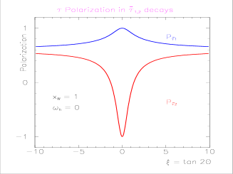
Figure 5: Polarization of the tau in the decay $\tilde{\tau}^{-}_{1,2}\to\tau^{-}\tilde{\chi}^{0}_{1}$ as a function of the stau mixing angle $\theta$ (which depends on $\tan\beta$) for bino-like $\tilde{\chi}^{0}_{1}$. From [16]

Moreover, if $A_{\tau}$ or $\mu$ turn out to be complex, the phase of the off-diagonal term $a_{\tau}m_{\tau}=({\ A_{\tau}}-{\ \mu}^{*}\tan\beta)m_{\tau}=|a_{\tau}m_{\tau}|{\rm e}^{i\Phi_{\tau}}$ modifies $\tilde{\tau}$ properties. Although the best would be to determine the complex parameters by measuring suitable $CP$ violating observables, this is not straightforward, because the $\tilde{\tau}_{i}$ are spinless and their main decay modes are two–body decays. However, the $CP$ conserving observables also depend on the phases.

For example, the various $\tilde{\tau}$ decay branching ratios depend in a characteristic way on the complex phases [17]. This is illustrated in Fig. 6.

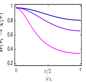
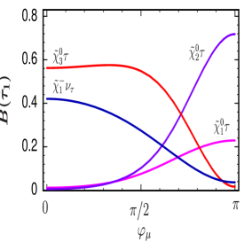
Figure 6: Branching ratios of $\tilde{\tau}_{1}$ and $\tilde{\tau}_{2}$ as a function of: $\varphi_{A_{\tau}}$ (left), $\varphi_{\mu}$ (right). From [17].

The fit to the simulated experimental data with 2 ab^-1 at a collider like TESLA shows that $\Im{\rm m}A_{\tau}$ and $\Re{\rm e}A_{\tau}$ can be determined with an error of order 10%.

Similarly, for the $\tilde{t}$ and $\tilde{b}$ sectors, the $L-R$ mixing can be important. By measuring the production cross sections with polarized beams the squark masses and mixing angles can be determined quite precisely [18], see Fig.7.

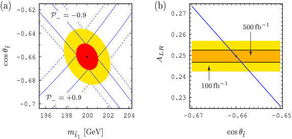
Figure 7: (a) Error bands and 68% CL ellipse in {$m_{\tilde{t}_{1}}$, $\cos\theta_{\tilde{t}}$} plane from cross section measurements; ${\int L}=100{\rm\ fb}^{-1}$ (dashes) and $500{\rm\ fb}^{-1}$ (solid). (b) The determination of $\cos\theta_{\tilde{t}}$ from $A_{LR}$. From [18].

For more details on the sfermion sector, we refer to [19]

3 Extrapolating to high-energy scale

Why we need high precision measurements? The Standard Model physics is characterized by energy scales of order 100 GeV. However we expect the origin of supersymmetry breaking at the high scale, near the Planck scale $\Lambda_{\rm PL}\sim 10^{19}$ GeV or the grand unification [GUT] scale $\Lambda_{GUT}\sim 10^{16}$ GeV. Information on physics near the Planck scale may become available from the well-controlled extrapolation of fundamental parameters measured with high precision at laboratory energies. Although such extrapolations exploiting renormalization group techniques extend over 13 to 16 orders of magnitude, they can be carried out in a stable way in supersymmetric theories [20]. Such a procedure has very successfully been pursued for the three electroweak and strong gauge couplings providing the solid base of the grand unification hypothesis.

This method can be expanded to a large ensemble of the soft SUSY breaking parameters: gaugino and scalar masses, as well as trilinear couplings. Recently this procedure has been applied [21] to the minimal supergravity (with a naturally high degree of regularity near the grand unification scale) and confronted with the gauge mediated supersymmetry breaking GMSB, see Fig.8.

The basic structure in this approach is assumed to be essentially of desert type, although the existence of intermediate scales is not precluded. An interesting example, the left-right extension of mSUGRA incorporating the seesaw mechanism for the masses of right-handed neutrinos, as well as a string-inspired effective field theory example, can be found in [21].

This bottom-up approach, formulated by means of the renormalization group, makes use of the low-energy measurements to the maximum extent possible. Therefore high-quality experimental data are necessary in this context, that should become available by future lepton colliders, to reveal the fundamental theory at the high scale.

a)    $M_{j}^{2}$ [GeV²]                               b)    $M_{j}^{2}$ [GeV²]

Figure 8: Evolution, from low to high scales, of first-generation sfermion mass parameters squared and the Higgs mass parameter $M^{2}_{H_{2}}$ for (a) the mSUGRA point SPS#1a, (b) the GMBS point SPS#8. The widths of the bands indicate the 1$\sigma$ CL. From [21].

4 Conclusions

Data rules! We need them badly. The LHC will provide plenty of data, however, their theoretical interpretation will be possible in specific models. In this context the $e^{+}e^{-}$ linear collider is very much welcome. Overlap of the LC running with the LHC would greatly help to perform critical tests: quantum numbers, masses, couplings etc. We have demonstrated that from the future high-precision data taken at $e^{+}e^{-}$ linear colliders, TESLA in particular, and combined with results from LHC, and CLIC later, the low-energy parameters of the supersymmetric model can be determined. Then the bottom-up approach, by evolving the parameters from the low-energy scale to the high scale by means of renormalization group techniques, can be exploited to reconstruct the fundamental supersymmetry parameters at the high scale, GUT or Planck, providing a picture in a region where gravity is linked to particle physics, and superstring theory becomes effective directly.

References

- [1] Talks by R. McPherson, by Y. Sirois and by T. Kamon, these Proceedings.
- [2] S. Ferrara, L. Girardello and F. Palumbo, Phys. Rev. D 20, 403 (1979).
- [3] L. Girardello and M. T. Grisaru, Nucl. Phys. B 194 (1982) 65.
- [4] For a recent discussion of CP phases see talk by P. Nath, these Proceedings and T. Ibrahim and P. Nath, arXiv:hep-ph/0210251, and references therein.
- [5] E. Accomando et al., ECFA/DESY LC Working Group, Phys. Rep. 299 (1998) 1; “TESLA Technical Design Report Part III: Physics at an e+e- Linear Collider”, eds. R. Heuer, D.J. Miller, F. Richard and P.M. Zerwas, DESY 01-011 and hep-ph/0106315.
- [6] For a summary see F. Paige, these Proceedings and arXiv:hep-ph/0211017, and references therein.
- [7] Talk by G. L. Kane, these Proceedings and arXiv:hep-ph/0210352.
- [8] J. Kalinowski, Acta Phys. Polon. B 30 (1999) 1921 [arXiv:hep-ph/9904260]; J.L. Kneur and G. Moultaka, Phys. Rev. D 61 (2000) 095003 [arXiv:hep-ph/9907360].
- [9] W. Majerotto, these Proceedings and arXiv:hep-ph/0209137, and references therein.
- [10] G.A. Blair and U. Martyn, Proceedings, LC Workshop, Sitges 1999, hep-ph/9910416.
- [11] S. Y. Choi, M. Guchait, J. Kalinowski and P. M. Zerwas, Phys. Lett. B 479 (2000) 235 [arXiv:hep-ph/0001175]. S.Y. Choi, A. Djouadi, M. Guchait, J. Kalinowski, H.S. Song and P.M. Zerwas, Eur. Phys. J. C 14 (2000) 535.
- [12] S.Y. Choi, J. Kalinowski, G. Moortgat-Pick and P.M. Zerwas, Eur. Phys. J. C 22 (2001) 563 [Addendum-ibid. C 23 (2002) 769].
- [13] Talks by A. Brandenburg, by G. Moortgat-Pick, by S. Hesselbach and by C. Hensel in Session 1B.
- [14] M. M. Nojiri, Phys. Rev. D 51 (1995) 6281 [arXiv:hep-ph/9412374]. M. M. Nojiri, K. Fujii and T. Tsukamoto, Phys. Rev. D 54 (1996) 6756 [arXiv:hep-ph/9606370].
- [15] A. Freitas, DESY-THESIS-2002-023. A. Freitas, D. J. Miller and P. M. Zerwas, Eur. Phys. J. C 21 (2001) 361 [arXiv:hep-ph/0106198].
- [16] E. Boos et al., arXiv:hep-ph/0211040.
- [17] A. Bartl, K. Hidaka, T. Kernreiter and W. Porod, Phys. Lett. B 538 (2002) 137 [arXiv:hep-ph/0204071]; arXiv:hep-ph/0207186.
- [18] A. Bartl, H. Eberl, S. Kraml, W. Majerotto and W. Porod, Eur. Phys. J. directC 2 (2000) 6 [arXiv:hep-ph/0002115].
- [19] Talks by E. Boos, by A. Freitas and by M.M. Nojiri in Session 1B.
- [20] E. Witten, Nucl. Phys. B 188 (1981) 513.
- [21] G.A. Blair, W. Porod and P.M. Zerwas, Phys. Rev. D 63 (2001) 017703; DESY 02-166 and hep-ph/0210058.