abstract Topological defects are involved in a plethora of physical and astrophysical phenomena. In these lectures, I will review the rôle they could play in the large-scale structure formation and the anisotropies of the cosmic microwave background, as well as in various high energy phenomena, including baryon number asymmetry, ultra-high energy cosmic rays, and gamma ray bursts. I will then summarize the gravitational effects of cosmic strings. Finally, I will briefly discuss the rôle of topological defects in brane world cosmology.

1 Introduction

Most aspects of high energy physics beyond the standard model can only be tested by going to very high energies, which are by far greater than those accessible by present, or even future, terrestrial accelerators. Cosmology has offered a way to experimentally test new theories of fundamental forces. In these lectures, I will shortly present the fascinating interplay between particle physics and cosmology, as provided by topological defects.

Many particle physics models of matter admit solutions which correspond to a class of topological defects, that are either stable or long-lived. Provided our understanding about unification of forces and the big bang cosmology are correct, it is natural to expect that such topological defects could have formed naturally during phase transitions followed by spontaneously broken symmetries, in the early stages of the evolution of the universe. Certain types of defects lead to disastrous consequences for cosmology and thus, they are undesired, while others may play a useful rôle.

Spontaneous symmetry breaking is an old idea, having its origin in the field of condensed matter physics, where it is described in terms of the order parameter, while in particle physics, symmetry breaking is described in terms of a scalar field, the Higgs field. The symmetry is called spontaneously broken (SSB) if the ground state is not invariant under the full symmetry of the Lagrangian density. Thus, the vacuum expectation value of the Higgs field is non-zero. In quantum field theories, broken symmetries are restored at high enough temperatures, as one can easily see from the finite temperature effective potential, which can be calculated from the zero temperature classical potential in loop expansion.

In three spatial dimensions, four different kinds of topological defects can arise. Whether or not topological defects will develop during a symmetry breaking phase transition as well as the determination of their type both depend on the topology of the vacuum manifold ${\cal M}$. The properties of ${\cal M}$ are usually described by the $n^{\rm th}$ homotopy group $\pi_{n}({\cal M})$ which classifies dinstinct mappings from the $n$-dimensional sphere $S^{n}$ into the manifold ${\cal M}$. If ${\cal M}$ has disconnected components, or equivalently if the order $n$ of the non-trivial homotopy group is $n=0$, then two-dimensional defects, called domain walls, form. The spacetime dimension $d$ of the defects is given in terms of the order of the non-trivial homotopy group by $d=4-1-n$. If ${\cal M}$ is not simply connected, in other words if ${\cal M}$ contains loops which cannot be continuously shrunk into a point, then cosmic strings form. A necessary, but not sufficient, condition for the existence of stable strings is that the first homotopy group (the fundamental group) $\pi_{1}({\cal M})$ of ${\cal M}$, must be non-trivial, or multiply connected. Cosmic strings are line-like defects, $d=2$. If ${\cal M}$ contains unshrinkable surfaces, then monopoles form, for which $n=2,~{}d=1$. Finally, if ${\cal M}$ contains non-contractible three-spheres, then textures form. Textures are event-like defects with $n=3,~{}d=0$.

Topological defects are called local or global. The energy of local defects is strongly confined, while the gradient energy of global defects is spread out over the causal horizon at defect formation.

In these lectures I will basically concentrate on cosmic strings, which have very intriguing properties and interesting cosmological implications [1, 2]. I will discuss the rôle which they could play in the large-scale structure and the anisotropies of the cosmic microwave background, as well as the rôle of cosmic strings in explaining various high energy phenomena. I will then summarize the gravitational effects of cosmic strings networks. Finally, I will discuss topological defects within brane world cosmology.

This review is organized as follows: In Section 2, I describe cosmic strings in the context of field theory. I first discuss two simple models, the abelian-Higgs model and the Goldstone model, which lead to local and global strings respectively. I then summarize string formation and string dynamics. After this short introduction to the physics of cosmic strings, I proceed with their physical/astrophysical consequences. In Section 3, I analyze the mechanism of cosmic structure formation with topological defects. I first describe the basic observable of the cosmic microwave background, and the physical mechanisms which are responsible for the microwave background anisotropies. I compare topological defects models versus inflationary ones, as the two alternative mechanisms for structure formation within gravitational instability theory. Concluding that topological defects are excluded as the main source of the large-scale structure, I address the question of finding the more natural class of inflationary models, meaning inflationary scenarios motivated by high energy physics. I then discuss the implications of these findings for particle physics models. In Section 4, I describe how cosmic strings could explain various high energy phenomena (baryon asymmetry, ultra-high energy cosmic rays, and gamma ray bursts). In Section 5, I discuss the gravitational effects of cosmic strings networks. In Section 6, I briefly comment on the rôle of topological defects in brane world cosmology. I close this review with the conclusions in Section 7.

2 Cosmic strings in field theory

In two simple cases, I describe how cosmic strings appear in the context of field theory. I first present the abelian-Higgs model and I then proceed with the Goldstone model for which the gauge fields are removed. I will not discuss non-abelian strings (e.g., $Z_{N}-$ strings, Alice strings, electroweak strings) which can arise at a symmetry breaking $G\rightarrow H$, with $G$ a non-abelian group, for which the unbroken subgroup $H$ is disconnected.

2.1 LOCAL OR GAUGE STRINGS

Let us consider the simplest example of a gauge field theory with SSB. This is the abelian-Higgs model with Lagrangian density

$${\cal L}=D_{\mu}{\bar{\phi}}D^{\mu}\phi-{1\over 4}F_{\mu\nu}F^{\mu\nu}-V(\phi)~{}~{},~{}~{}V(\phi)={\lambda\over 4}(|\phi|^{2}-\eta^{2})^{2}~{},$$ (1)

where $D_{\mu}=\partial_{\mu}+ieA_{\mu}$ and $F_{\mu\nu}=\partial_{\mu}A_{\nu}-\partial_{\nu}A_{\mu}$. The $U(1)$ invariance is satisfied by the transformations $\phi\rightarrow\phi\exp[i\alpha(x)]$,  $A_{\mu}\rightarrow A_{\mu}-(1/e)\partial_{\mu}\alpha(x)$, where $\alpha(x)$ is a real single-valued function with a spatial dependence.

The Euler-Lagrange equations, which follow from Eq. (1), read

$$[D^{2}+\lambda(|\phi|^{2}-\eta^{2})]\phi=0~{}~{},~{}~{}\partial_{\nu}F^{\mu\nu}+ie({\bar{\phi}}D^{\mu}\phi-D^{\mu}{\bar{\phi}}\phi)=0~{}.$$ (2)

We are seeking a cylindrically symmetric, static solution of the above field equations. In cylindrical polar cordinates $\{\rho,\varphi,z\}$, we demand the solution to approach a vacuum state as $\rho\rightarrow\infty$, meaning that $\phi\rightarrow\eta\exp(in\varphi)$ (with $n$ an integer) and $A_{\mu}\rightarrow(n/e)\partial_{\mu}\varphi$, thus $D_{\mu}\phi\rightarrow 0$. We make the ansatz:

$$\phi = \eta f(\rho)\exp(in\varphi)$$

$$A_{x} = {-n\eta\over e}\left({y\over\rho^{2}}\right)\alpha(\rho)$$

$$A_{y} = {n\eta\over e}\left({x\over\rho^{2}}\right)\alpha(\rho)$$

$$A_{z} = 0~{},$$ (3)

which we insert into the field equations and we get two coupled ordinary differential equations for $f$ and $\alpha$. Solutions to this system, describing a string along the $z$-axis and satisfying the requirements $f(0)=\alpha(0)=0$, and $f(\rho)~{},~{}\alpha(\rho)\rightarrow 1$ as $\rho\rightarrow 1$, can be found numerically.

The string solution of the abelian-Higgs model is the Nielsen-Olesen vortex [3]. For a local string, the energy per unit length is finite. For large $\rho$, the energy per unit length of the gauge string, $\mu=\int\rho d\rho d\varphi T_{0}^{0}$, is of the order of $\mu\sim 2\pi\eta^{2}$. The local string also contains a tube of magnetic flux, with quantized flux $(2\pi n/e)$.

The thickness of a Nielsen-Oleson string is about $1/\eta$ and on length scales which are much larger than $1/\eta$, its energy momentum tensor can be approximated by

$$(T_{\mu}^{\nu})=\mu\delta(x)\delta(y){\rm diag}(1,0,0,1)~{}.$$ (4)

The vortices in the abelian-Higgs model have as condensed matter analogues, the flux tubes in superconductors.

2.2 GLOBAL STRINGS

Let us consider a complex scalar field $\phi(x)$, described by the Lagrangian density

$${\cal L}={1\over 2}\partial_{\mu}\phi\partial^{\mu}\bar{\phi}-V(\phi)~{}~{},~{}~{}V(\phi)={\lambda\over 4}(|\phi|^{2}-\eta^{2})^{2}~{}.$$ (5)

We remain at low temperatures, so we only consider the zero temperature effective potential, while we do not include any thermal corrections. The Lagrangian density, Eq. (5), has a global $U(1)$ symmetry, under the transformation $\phi\rightarrow\phi\exp(i\tilde{\alpha})$, with $\tilde{\alpha}$ constant.

The Euler-Lagrange equations that follow from Eq. (5) read

$$[\partial^{2}+\lambda(|\phi|^{2}-\eta^{2})]\phi=0~{}.$$ (6)

Thus, the vacuum manifold is a circle of radius $\eta$. At high enough temperatures, $T\gg\eta$, the effective potential has a single minimum located at $\phi=0$. However, as the temperature falls below a critical value $T_{\rm c}$, with $T_{\rm c}\sim\eta$, a phase transition occurs and the field $\phi$ takes a non-zero vacuum expectation value, $\langle 0|\phi|0\rangle=\eta\exp(i\alpha_{0})$, where $\alpha_{0}$ is a constant. This ground state solution is stable, and since it does not remain invariant under the $U(1)$ symmetry transformations, the symmetry is said to be broken by the vacuum.

Besides the vacuum, there are also static solutions with non-zero energy density. In cylindrical polar coordinates $\{\rho,\varphi,z\}$, we make the ansatz:

$$\phi({\bf x})=\eta\tilde{f}(\rho)~{}\exp(in\varphi)$$ (7)

(with $n$ an integer). The field equations of motion reduce to a single non-linear ordinary differential equation for $\tilde{f}$. As $\rho\rightarrow 0$, continuity of $\phi$ demands $\tilde{f}\rightarrow 0$, while at infinity, $\tilde{f}\rightarrow 1$, so that $\phi\rightarrow|\phi|=\eta$. These solutions are known as global strings or vortices  [4, 5], and they have close analogies with the vortices in superfluid ⁴He [6, 7].

The non-zero components of the vortex energy momentum tensor are

$$T_{0}^{0}=T_{z}^{z}=|\dot{\phi}^{2}|+V(\phi)+|{\bf\nabla}\phi|^{2}=-{\lambda\eta^{4}\over 2}\left[\tilde{f}^{{}^{\prime}2}-{1\over 2}(\tilde{f}^{2}-1)^{2}+{\eta^{2}\over\lambda\eta^{2}\rho^{2}}\tilde{f}^{2}\right]$$ (8)

The energy per unit length of cross-section of a vortex of radius $R$ is

$$\mu(R)=2\pi\int_{0}^{R}~{}T_{0}^{0}~{}\rho~{}{\rm d}\rho~{}\sim~{}\pi\eta^{2}\ln(\sqrt{\lambda}\eta R)~{}.$$ (9)

The logarithmic divergence for large $R\gg(\sqrt{\lambda}\eta)^{-1}$, comes from the angular part of the gradient term, the last term in Eq. (8), which decays only as $1/\rho^{2}$. Clearly an upper cutoff is naturally provided by either the curvature radius of the string or by its distance to the next vortex.

The energy per unit length of local strings was found to be finite, since the angular derivative of the field was replaced by a covariant derivative, which can vanish faster than $1/\rho$ at infinity. The energy density of local strings was found to be much more localized than in the global string case.

I will now discuss the formation and dynamics of cosmic strings, making no distinction between local/global strings.

2.3 FORMATION OF STRINGS

According to the laws of standard cosmology, our universe in the past was denser and hotter. Thus, the early universe was in a symmetric phase and there were no topological defects. As the universe expands, it cools down and once its temperature falls below a critical value $T_{\rm c}$, the Higgs field settles down into the valley of the minima of the potential. Eventually, as the temperature drops to zero, the system tends towards one of the equivalent vacuum states and the original symmetry is broken.

The density of defects depends on the order of the phase transition. In the original picture [8], defects form at a second-order phase transition and their density is determined by the correlation length $\xi(T_{\rm f})$ of the Higgs field $\phi$ at the freeze-out temperature $T_{\rm f}$, which is identified with the Ginzburg temperature $T_{\rm G}$. The correlation length $\xi(T)$ sets the maximum distance over which the Higgs field can be correlated during a symmetry breaking phase transition. The Ginzburg temperature $T_{\rm G}$ is the temperature below which thermal fluctuations cannot restore the broken symmetry at the scale of the correlation length. Since the horizon distance is finite, at the time of phase transition the Higgs field must be uncorrelated on scales greater than the particle horizon, which sets an absolute maximum for the correlation length. As a result, non-trivial vacuum configurations will necessarily be produced during a symmetry breaking phase transition in the early universe, with an abundance of order one per horizon volume. This original picture has been later revised, as I will now discuss.

For given temperature $T$, the time $\tau(T)$ it takes to correlations to establish on the length scale $\xi(T)$, has a rather crucial rôle [9, 10]. As $T\rightarrow T_{\rm c}$, both $\xi(T)$ and $\tau(T)$ diverge as inverse powers of $(T-T_{\rm c})$. Once $\tau(T)$ exceeds the dynamical time scale $t_{\rm D}=|T-T_{\rm c}|/|\dot{T}|$ of the temperature variation, then correlations cannot establish on larger scales. Thus, the freeze-out temperature $T_{\rm f}$ should be determined by $\tau\sim t_{\rm D}$ and this is known as the Kibble-Zurek picture [9, 10, 11]. In this picture of defect formation, the distribution of defects is determined by the distribution of zeros of the Higgs field $\phi$, smoothed over the correlation length $\xi$, in thermal equilibrium at the freeze-out temperature $T_{\rm f}$. This picture is supported by experiments in ${}^{3}He$, by non-equilibrium quantum field theory studies, as well as by numerical simulations. However, despite all this, defect formation in second-order phase transitions still remains an open issue.

On the other hand, if defects were formed as a result of a first-order phase transition, then their density depends on how efficient is phase equilibration in bubble collisions. It turns out that the physics of defect formation in bubble collissions is quite involved and one cannot just use a simple rule in order to estimate the density of defects. I will not enter into any details and I refer the reader to the literature [12, 13, 14, 15, 16].

In the case of cosmic strings, energetics do not determine the phase of the vacuum expectation value of the complex Higgs field $\phi$, since the vacuum energy depends only upon $|\phi|$, while the phase is arbitrary. Since $\phi$ must be single valued, the total change in phase around any closed path must be an integer multiple of $2\pi$. Imagine a closed path with total change in phase equal to $2\pi$. As the path is shrunk to a point, the total change in phase cannot change continuously from $2\pi$ to $0$. Thus, there must be one point inside the path where the phase is undefined, meaning that the vacuum expectation value of $\phi$ vanishes. The region of false vacuum inside this path is part of a tube of false vacuum, the cosmic string. Cosmic strings must be either infinite in length or closed in form of loops, since otherwise it would be possible to deform the path around the tube and contract it to a point without encountering the tube of false vacuum. Assuming that the radius of curvature of a string is much greater than its thickness, cosmic strings can be considered as one-dimensional, in space, objects.

2.4 STRING DYNAMICS

The world history of a string can be expressed by a two-dimensional surface in the four-dimensional spacetime, which is called the string worldsheet:

$$x^{\mu}=x^{\mu}(\zeta^{a})~{}~{},~{}~{}a=0,1$$ (10)

where the worldsheet coordinates $\zeta^{0},\zeta^{1}$ are arbitrary parameters chosen so that $\zeta^{0}$ is timelike and $\zeta^{1}$ spacelike.

The string equations of motion, in the limit of strings of zero thickness, are derived from the Nambu-Goto action which, up to an overall factor, corresponds to the surface area swept out by the string in spacetime:

$$S=-\mu\int\sqrt{-\gamma}d^{2}\zeta~{},$$ (11)

where $\gamma$ is the determinant of the two-dimensional worldheet metric $\gamma_{ab}$,

$$\gamma={\rm det}(\gamma_{ab})={1\over 2}\epsilon^{ac}\epsilon^{bd}\gamma_{ab}\gamma_{cd}~{}~{},~{}~{}\gamma_{ab}=g_{\mu\nu}x^{\mu}_{,a}x^{\nu}_{,b}$$ (12)

with $g_{\mu\nu}$ the four-dimensional metric.

Varying the Nambu-Goto action with respect to $x^{\mu}(\zeta^{a})$ we obtain the string equations of motion

$$x^{\mu~{};a}_{,a}+\Gamma^{\mu}_{\nu\sigma}\Gamma^{ab}x^{\nu}_{,a}x^{\sigma}_{,b}=0~{},$$ (13)

with $\Gamma^{\mu}_{\nu\sigma}$ the four-dimensional Christoffel symbol.

The string energy-momentum tensor can be found by varying the Nambu-Goto action with respect to the metric $g_{\mu\nu}$:

$$T^{\mu\nu}\sqrt{-g}=\mu\int d^{2}\zeta\sqrt{-\gamma}\gamma^{ab}x^{\mu}_{,a}x^{\nu}_{,b}\delta^{(4)}(x^{\sigma}-x^{\sigma}(\zeta^{a}))~{}.$$ (14)

One then distinguishes between strings in flat or in curved spacetime, fix the gauge conditions, find the string equations of motion, and solve them.

The Nambu-Goto action, Eq. (11), describes the string motion in the absence of string intersections with itself or another string. At least within simple models, strings cannot simply pass through one another with no interaction, so strings reconnect. At every intercommuting, string pieces moving originaly independently from each other, become connected. At the intersection time, ${\bf x}^{\prime}$ and $\dot{\bf x}$ change very rapidly as functions of $\zeta^{1}$ on a length scale which is comparable to the thickness of the string. The region of this rapid change is known as kink, and at the kink, ${\bf x}^{\prime}$ and $\dot{\bf x}$ are discontinuous. Closed loops of string can self-intersect and break into smaller loops.

For many years, the evolution of a string network was described in the basis of the one-scale model [11], which gives long-string evolution in terms of a correlation length , given two free parameters, the loop chopping efficiency and the root-mean-square velocity. However, strings in an interacting network develop substantial substructure in the form of kinks and wiggles, on a smaller scale than the characteristic length scale of the network. Numerical studies [17, 18] have revealed the wiggliness of the long strings and have demonstrated the inedequacy of the one-scale model. As a result, the three-scale model has been proposed [19]. A numerical study of the three-scale model emphasizing the important dependence of small-scale structure on the numerical loop cutoff has been presented in Ref.[20].

In the next sections I will discuss the possible rôle of cosmic strings on various cosmological and astrophysical issues.

3 Cosmic structure formation with topological defects

The geometry of our universe is to a very good approximation isotropic, and assuming that we are not in a special position, then it is also homogeneous. The best observational evidence in support to this is the isotropy of the cosmic microwave background (CMB). The CMB, last scattered at the epoch of decoupling, has to a high accuracy a black-body distribution [21, 22], with a temperature $T_{0}=2.728\pm 0.002~{}{\rm K}$, which is almost independent of direction. The DMR experiment on the COBE satellite measured a tiny variation $\Delta T$ in intensity of the CMB, at fixed frequency. This is equivalently expressed as a variation in the temperature, which was measured [23, 24] to be $\Delta T/T_{0}\approx 10^{-5}$. On the other hand, on galaxy and cluster scales the matter distribution is very inhomogeneous.

The origin of the large-scale structure in the universe, remains one of the most important questions in cosmology. Within the framework of gravitational instability, two families of models attempted to explain the formation of the structure one observes. Initial density perturbations can either be due to freezing in of quantum fluctuations of a scalar field during an inflationary period, or they may be seeded by a class of topological defects, which could have formed naturally during a symmetry breaking phase transition in the early universe. The CMB anisotropies provide a link between theoretical predictions and observational data, which may allow us to distinguish between inflationary models and topological defects scenarios, by purely linear analysis. More precisely, the characteristics of the CMB anisotropy multipole moments (position, amplitude of acoustic peaks), and the statistical properties of the CMB anisotropy are used to discriminate among models, and to constrain the parameters space [25].

3.1 OBSERVABLES OF THE CMB

The basic observable is the CMB intensity as a function of frequency and direction of observation $\hat{{\bf n}}$. We want to calculate temperature anisotropies in the sky, thus it is natural to expand $\Delta T/T_{0}$ in spherical harmonics:

$${\Delta T\over T_{0}}(\hat{{\bf n}})=\sum_{\ell=1}^{\infty}\sum_{m=-\ell}^{m=\ell}a_{\ell m}Y_{\ell m}(\hat{{\bf n}}){\cal W}_{\ell}~{},$$ (15)

where $\Delta T=T-T_{0}$, with $T_{0}$ the mean temperature in the sky, and ${\cal W}_{\ell}$ stands for the $\ell$-dependent window function of the particular experiment.

The angular power spectrum of CMB anisotropies is expressed in terms of the dimensionless coefficients $C_{\ell}$, which is the ensemble average of the coefficients $a_{\ell m}$:

$$C_{\ell}=\langle|a_{\ell m}|^{2}\rangle~{}.$$ (16)

If the fluctuations are statistically isotropic, then $C_{\ell}$’s are independent of $m$, and if they are Gaussian, then all the statistical information is contained in the power spectrum. Topological defects generate non-Gaussian perturbations, while one-field inflation leads, in general, to Gaussian perturbations. Departure from the vacuum initial conditions for cosmological perturbations of quantum mechanical origin leads generically to a non-Gaussian signature, however the signal-to-noise ratio is far away from experimental detection [26, 27]. In what follows when I refer to perturbations of quantum-mechanical origin, I will simply consider as initial state to be the vacuum.

The relation between the power spectrum and the two-point correlation function is:

$$\left\langle{\Delta T\over T_{0}}(\hat{{\bf n}}_{1}){\Delta T\over T_{0}}(\hat{{\bf n}}_{2})\right\rangle={1\over 4\pi}\sum_{\ell}(2\ell+1)C_{\ell}P_{\ell}(\hat{{\bf n}}_{1}\cdot\hat{{\bf n}}_{2})~{},$$ (17)

where $P_{\ell}$ denotes the Legendre polynomials. The angular power spectrum compares points in the sky separated by an angle $\vartheta$, where $(\hat{{\bf n}}_{1}\cdot\hat{{\bf n}}_{2})=\cos\vartheta$. Here the brackets denote spatial average, or expectation values if perturbations are quantized. The value of $C_{\ell}$ is determined by fluctuations on angular scales of order $2\pi/\ell$.

In a real experiment, we have only one universe and one sky, and therefore we cannot measure an ensemble average. Assuming statistical isotropy,

$$C_{\ell}\simeq C_{\ell}^{\rm obs}={1\over 2\ell+1}\sum_{m}|a_{\ell m}|^{2}~{},$$ (18)

which in the ideal case of full sky coverage, this yields an average on $2\ell+1$ numbers. Assuming that the temperature fluctuations are Gaussian, the observed mean deviates from the ensemble average by about

$${\sqrt{(C_{\ell}^{\rm obs})^{2}-(C_{\ell})^{2}}\over C_{\ell}}\simeq\sqrt{{2\over 2\ell+1}}~{}.$$ (19)

This limitation of the precision of a measurement is known as cosmic variance and it is important especially for low multipoles.

3.2 PHYSICS OF THE CMB

Since the distribution of photons is uniform, perturbations are small, and they can be studied with linear perturbation theory. One can split perturbations into scalar, vector and tensor modes; different components do not mix. Initially vector perturbations rapidly decay, while scalar and tensor perturbations contribute to the CMB. At the time of recombination ($T_{\rm rec}\sim 3000K$, $z_{\rm rec}\approx 10^{3})$, electrons and protons formed neutral hydrogen. Earlier, free electrons acted as glue between the photons and the baryons through Thomson and Coulomb scattering, implying that the cosmological plasma was a tightly coupled photon-baryon fluid. After recombination, the universe becomes transparent for CMB photons, and they move along geodesics of the perturbed Friedmann geometry.

Integrating the perturbed geodesic equation, temperature anisotropies in gauge-invariant form take the form [28, 29, 30]:

$$\left({\Delta T\over T}\right)^{({\rm s})}(\eta_{0},{\bf x}_{0},{\hat{\bf n}}) = {1\over 4}D_{\rm r}(\eta_{\rm dec},{\bf x}_{\rm dec})+v_{i}(\eta_{\rm dec},{\bf x}_{\rm dec})n^{i}$$

$$+(\Phi-\Psi)(\eta_{\rm dec},{\bf x}_{\rm dec})-\int_{\eta_{\rm dec}}^{\eta_{0}}(\dot{\Phi}-\dot{\Psi})(\eta,{\bf x}(\eta)){\rm d}\eta$$

$$\left({\Delta T\over T}\right)^{({\rm t})}(\eta_{0},{\bf x}_{0},{\hat{\bf n}}) = -\int_{\eta_{\rm dec}}^{\eta_{0}}\dot{h}_{ij}(\eta,{\bf x}(\eta))n^{i}n^{j}{\rm d}\eta~{},$$ (20)

where $\eta$ denotes conformal time; ${\bf x}(\eta)$ is the comoving unperturbed photon position at time $\eta$; $D_{\rm r}$ is the photon energy density fluctuations; $v_{i}$ is the baryon velocity field; $\Phi,\Psi$ are the Bardeen potentials, an overdot denotes derivative with respect to conformal time $\eta$; and $h_{ij}$ is a spatial metric perturbation (tracelless $\delta^{ij}h_{ij}=0$ and transverse $\vartheta_{i}h_{ij}=0$).

Let us take the scalar mode of temperature anisotropies, which is the first of Eqs. (20). The first term describes the intrinsic inhomogeneities on the surface of the last scattering due to acoustic oscillations prior to decoupling. It also contains contributions to the geometrical perturbations. The second term describes the relative motions of emitter and observer. This is the Doppler contribution to the CMB anisotropies. It appears on the same angular scale as the acoustic term and we denote the sum of the acoustic and Doppler contributions by acoustic peaks. The last two terms are due to the inhomogeneities in the space-time geometry; the first contribution determines the change in the photon energy due to the difference of the gravitational potential at the position of emitter and observer. Together with the part contained in $D_{\rm r}$ they represent the ordinary Sachs-Wolfe effect. The second term accounts for red-shifting or blue-shifting caused by the time dependence of the gravitational field along the path of the photon (Integrated Sachs-Wolfe (ISW) effect). The sum of the two terms is the full Sachs-Wolfe contribution (SW).

On angular scales $0.1^{\circ}\stackrel{{\scriptstyle<}}{{\sim}}\theta\stackrel{{\scriptstyle<}}{{\sim}}2^{\circ}$, the main contribution to the CMB anisotropies comes from the acoustic peaks, while the SW effect is dominant on large angular scales. For topological defects models, the gravitational contribution is mainly due to the ISW; the ordinary Sachs-Wolfe term even has the wrong spectrum, a white noise spectrum instead of a Harrison-Zel’dovich [31] spectrum.

On scales smaller than about $0.1^{\circ}$, the anisotropies are damped due to the finite thickness of the recombination shell, as well as by photon diffusion during recombination (Silk damping). Baryons and photons are very tightly coupled before recombination and oscillate as one component fluid. During the process of decoupling, photons slowly diffuse out of over-dense into under-dense regions. To fully account for this process, one has to solve the Boltzmann equation.

3.3 Topological defects models versus inflationary ones

Inflationary fluctuations are produced at a very early stage of the evolution of the universe, and are driven far beyond the Hubble radius by inflationary expansion. Subsequently, they are not altered anymore and evolve freely according to homogeneous linear perturbation equations until late times. These fluctuations are termed passive and coherent. Passive, since no new perturbations are created after inflation; coherent since randomness only enters the creation of perturbations during inflation, subsequently they evolve in a deterministic and coherent manner.

Within inflation, the induced perturbations are adiabatic density perturbations, meaning that the density of each particle species is a unique function of the total energy density $(\delta\rho_{\rm m}/\rho_{\rm m})=(3/4)(\delta\rho_{\rm r}/\rho_{\rm r})$.

The main difference in linear cosmological perturbation theory for models with topological defects, as compared to the adiabatic inflationary case, is that perturbations are generated by seeds (sources). The seeds are defined as any non-uniformly distributed form of energy, which contributes only a small fraction to the total energy density of the universe and which interacts with the cosmic fluid only gravitationally. Topological defects are a concrete example of such seeds. The energy momentum tensor of the seeds enters in the perturbation equation as a source term on the rhs, while the seeds themselves evolve according to the background space-time; perturbations in the seed evolution are of second order.

Topological defects (and in general models with seeds) lead to isocurvature density perturbations, in the sense that the total density perturbation vanishes, but those of the individual particle species do not. In other words, there is a non-zero temperature perturbation $S=(\delta\rho_{\rm m}/\rho_{\rm m})-(3/4)(\delta\rho_{\rm r}/\rho_{\rm r})\neq 0$, To have isocurvature perturbations, the universe has to possess more than the single degree of freedom provided by the total energy density. For isocurvature perturbations, the measure of the spatial curvature seen by comoving observers is zero, ${\cal R}=0$, during RDE, but on large scales entering the horizon during MDE, ${\cal R}=(1/3)S$.

In models with topological defects, fluctuations are generated continuously and evolve according to inhomogeneous linear perturbation equations. The energy momentum tensor of defects is determined by the their evolution which, in general, is a non-linear process. These perturbations are called active and incoherent. Active since new fluid perturbations are induced continuously due to the presence of the defects; incoherent since the randomness of the non-linear seed evolution which sources the perturbations can destroy the coherence of fluctuations in the cosmic fluid. The highly non-linear structure of the topological defects dynamics makes the study of the evolution of these causal (there are no correlations on super-Horizon scales) and incoherent initial perturbations much more complicated.

Among the various topological defects, local cosmic strings or any kind of global defects could, in principle, induce the initial perturbations. Models with domain walls or local monopoles are ruled out. In the first case, because even a single domain wall stretching across the present universe would overclose it, while in the second one, since local monopoles soon dominate the energy density of the universe due to the lack of interactions. Finally, textures cannot exist as local coherent defects which have a non-vanishing gradient energy. On the other hand, as it was shown from numerical simulations [18], a network of local cosmic strings approaches a scaling distribution, meaning that once scaling has been reached, there only be a few long strings crossing each Hubble volume, together with a distribution of rather small closed loops of strings. Thus, cosmic strings are not cosmologically undesirable. Global defects are also acceptable as possible candidates for a scenario of structure formation, since there are long range forces between them resulting to a scaling solution, in the sense that there is again a fixed number of such defects per Hubble volume.

The measurements of cosmic microwave background anisotropy by the COBE-DMR experiment provide the normalization $T_{\rm c}^{2}/M_{\rm Pl}\sim 10^{-5}$, where $T_{c}$ denotes the temperature at the symmetry breaking phase transition which gave rise to the topological defects, within a scenario of structure formation via a mechanism of seeds. Thus, to seed the observed large scale structure, global defects or local cosmic strings should have been formed at $T_{\rm c}\sim 10^{16}$ GeV, which is the scale of unification of weak, strong and electromagnetic interactions.

Within linear cosmological perturbation theory, structure formation induced by seeds is determined by the solution of the inhomogeneous equation

$$\mbox{$\cal D$}X({\bf k},t)=\SS({\bf k},t)~{},$$ (21)

where $X$ is a vector containing all the background perturbation variables for a given mode specified by the wave-vector ${\bf k}$, like the $a_{lm}$’s of the CMB anisotropies, the dark matter density fluctuation, the peculiar velocity potential etc., $\cal D$ is a linear time-dependent ordinary differential operator, and the source term $\SS$ is given by linear combinations of the energy momentum tensor of the seed (the type of topological defects we are considering). The generic solution of this equation is given in terms of a Green’s function and has the following form [32]

$$X_{i}({\bf k},t_{0})=\int_{t_{in}}^{t_{0}}\mbox{$\cal G$}_{il}({\bf k},t_{0},t)\SS_{l}({\bf k},t)dt~{}.$$ (22)

At the end, we need to determine expectation values, which are given by

$$\langle X_{i}({\bf k},t_{0})X_{j}({\bf k},t_{0})^{*}\rangle=\int_{t_{in}}^{t_{0}}\int_{\eta_{in}}^{\eta_{0}}\mbox{$\cal G$}_{il}(t_{0},t)\mbox{$\cal G$}_{jm}^{*}(t_{0},t^{\prime})\langle\SS_{l}(t)\SS_{m}^{*}(t^{\prime})\rangle dtdt^{\prime}.$$ (23)

Thus, the only information we need from topological defects simulations in order to determine cosmic microwave background and large-scale structure power spectra, is the unequal time two-point correlators [33], $\langle\SS_{l}(t)\SS_{m}^{*}(t^{\prime})\rangle$, of the seed energy-momentum tensor. This problem can, in general, be solved by an eigenvector expansion method [34].

A crucial issue, is how to reach the desirable dynamical range in order to compute accurately observables which will then be compared to the data. To overcome this difficulty, one applies the theoretical requirements of causality, scaling, and statistical homogeneity and isotropy.

The complexity of computations in defect scenarios has of course affected the number of studies, in which the mechanism of structure formation is provided by seeds, as compared to the inflationary case. Nevertheless, one can find in the literature scenario with global defects or local cosmic strings, as well as models with causal seeds which attempt to imitate inflation. Let us summarize the present status, once we compare theoretical predictions with the available data.

On large angular scales ($\ell\raise 1.72218pt\hbox{$<$}\kern-8.00003pt\lower 2.6694pt\hbox{$\sim$}50$), defect models lead to the same prediction as inflation, namely, they both predict an approximately scale-invariant (Harrison-Zel’dovich) spectrum of perturbations. Their only difference concerns the statistics of the induced fluctuations. Inflation predicts generically Gaussian fluctuations, whereas in the case of topological defects models, even if initially the defect energy-momentum tensor would be Gaussian, non-Gaussianities will be induced from the non-linear defect evolution. Thus, in defect scenarios, the induced fluctuations are non-Gaussian, at least at sufficiently high angular resolution. This is an interesting fingerprint, even though difficult to test through the data.

On itermediate and small angular scales however, the predictions of models with seeds are quite different than those of inflation, due to the different nature of the induced perturbations. In topological defects models, defect fluctuations are constantly generated by the seed evolution. The non-linear defect evolution and the fact that the random initial conditions of the source term in the perturbation equations of a given scale leak into other scales, destroy perfect coherence. The incoherent aspect of active perturbations does not influence the position of the acoustic peaks, but it does affect the structure of secondary oscillations, namely secondary oscillations may get washed out. Thus, in topological defects models, incoherent fluctuations lead to a single bump at smaller angular scales (larger $\ell$), than those predicted within any inflationary scenario. This incoherent feature is shared in common by local and global defects.

Studying the acoustic peaks for perturbations induced by global textures, we found [35] that the amplitude of the first acoustic peak is only $\sim 1.5$ times higher than the SW plateau and its position is at $\ell\sim 350$. Global ${\cal{O}}(N)$ textures in the large $N$ limit show a flat spectrum, with a slow decay after $\ell\sim 100$ [36]. There are similar results with other global ${\cal{O}}(N)$ defects [37, 34]. For local cosmic strings the predictions range from an almost flat spectrum to a single wide bump at $\ell\sim 500$ with extremely rapidly decaying tail [38, 39, 40, 41, 42]. This discrepancy between global and local defects may come from the larger difference between the energy-momentum tensor in the radiation and matter-dominated era of the local defects, as compared to the case of global defects. Moreover, it seems that the microphysics of the cosmic string network plays a crucial role in the height and in the position of the bump. It is interesting to mention that in the case of local cosmic strings, the energy density is clearly dominant over the other components of the energy-momentum tensor, whereas this feature is not shared by global defects. In addition, the angular cosmic microwave background power spectrum of local cosmic strings depends on the equation of state of the decay product.

One expects also to find a defect fingerprint on the power spectrum of polarization. Due to the presence of vector perturbations, all defect models predict a much larger component of magnetic-type polarization on small angular scales, as compared to a standard cold dark matter model. In addition, the isocurvature shift of the acoustic peaks, as well as the incoherent character of the perturbations, appear in the polarization signal.

Standard inflation predicts the position of the first peak at $\ell\sim 220$ and its amplitude $\sim(4-6)$ times higher than the SW plateau.

One can manufacture models [43] with structure formation being induced by scaling seeds, which lead to an angular power spectrum with the same characteristics (position and amplitude of acoustic peaks), as the one predicted by standard inflationary models. The open question is, though, whether such models are the outcome of a realistic theory. At this point, I would like to remind to the reader that the question whether or not inflationary models which fit the data are physical or not, has also to be addressed, even though people often tend to forget about it.

I would also like to briefly mention another model, which could account for the origin of the large-scale curvature perturbation in our universe. This is the so-called curvaton model [44], where the curvaton is a scalar field which remains light during inflation, and gets perturbed with an almost scale-invariant spectrum. Initially there is an isocurvature density perturbation, which generates the curvature perturbation later, when the curvaton density becomes a significant fraction of the total. A priori this model can be applied in scenarios with seeds.

The position and amplitude of the acoustic peaks, as found by the CMB measurements — and in particular by the BOOMERanG [45, 46], MAXIMA [47, 48], and DASI [49, 50] experiments — are in disagreement with the predictions of topological defects models. Thus, the latest CMB anisotropy measurements rule out pure topological defects models as the origin of initial density fluctuations.

The inflationary paradigm is at present the most appealing candidate for describing the early universe. However, inflation is not free from open questions and I would like to mention the following three types of issues, to which any inflationary model should give an answer:
(i)It is difficult to implement inflation in high energy physics. More precisely, the inflaton potential coupling constant must be very low in order to reproduce the CMB data. This is related to the question of deciding which kind of inflationary model is the more natural one.
(ii) The quantum fluctuations are typically generated from sub-Planckian scales and therefore one should examine the validity of the theoretical predictions based upon standard quantum mechanics. Recent studies [51] seem to indicate that inflation is robust to some changes of the standard laws of physics beyond the Planck scale.
(iii) It is almost always assumed that the initial state of the perturbations is the vacuum. The proof of such a hypothesis, if it exists, should rely on full quantum gravity, a theory which is still lacking. If the initial state is not the vacuum, this would imply a large energy density of inflaton field quanta, not of a cosmological term type [52]. Thus, non-vacuum initial states lead to a back-reaction problem, which has not been calculated yet.

Since inflation provides, at present, the most appealing candidate for describing the early universe, we face the choice of the more physical inflationary scenario. Following the philosophy that the more natural cosmological model is the one which arises from particle physics models, as for example superstring theories, we will see that topological defects, and in particular cosmic strings, can still play a rôle for the origin of the large-scale structure and the patterns of cosmic microwave sky. I will thus comment on a new degeneracy apparently arising in the CMB data, that would be due to a small — but still significant — contribution of topological defects.

In many particle physics based models, inflation ends with the formation of topological defects, and in particular cosmic strings [53, 54, 55]. Moreover, cosmic strings are predicted by many realistic particle physics models. Thus, even though the current CMB anisotropy measurements seem to rule out the class of generic topological defects models as the unique mechanism responsible for the CMB fluctuations, it is conceivable to consider a mixed perturbation model, in which the primordial fluctuations are induced by inflation with a non-negligible topological defects contribution.

We consider [56] a model in which a network of cosmic strings evolved independently of any pre-existing fluctuation background, generated by a standard cold dark matter with a non-zero cosmological constant ($\Lambda$CDM) inflationary phase. As we shall restrict our attention to the angular spectrum, we are in the linear regime. Thus,

$$C_{\ell}=\alpha C^{\scriptscriptstyle{\rm I}}_{\ell}+(1-\alpha)C^{\scriptscriptstyle{\rm S}}_{\ell}~{},$$ (24)

where $C^{\scriptscriptstyle{\rm I}}_{\ell}$ and $C^{\scriptscriptstyle{\rm S}}_{\ell}$ denote the (COBE normalized) Legendre coefficients due to adiabatic inflation fluctuations and those stemming from the string network respectively. The coefficient $\alpha$ in Eq. (24) is a free parameter giving the relative amplitude for the two contributions. We have to compare the $C_{\ell}$, given by Eq. (24), with data obtained from CMB anisotropy measurements.

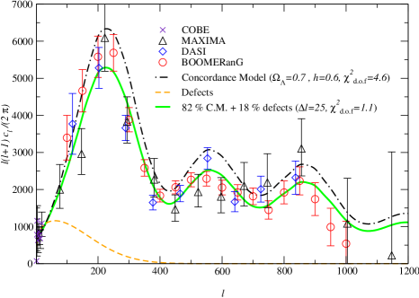
Figure 1.  : $\ell(\ell+1)C_{\ell}$ versus $\ell$ for three different models. The upper dot-dashed line represents the prediction of a $\Lambda$CDM model, with $n_{\rm S}=1$, $\Omega_{\Lambda}=0.7$, $\Omega_{\rm m}=0.3$, $\Omega_{\rm b}=0.05$ and $h=0.6$. The lower dashed line is a typical string spectrum. Both lines are normalized at the COBE scale (crosses). Combining both curves with the parameter $\alpha$ produces the solid curve, with a $\chi^{2}$ per degree of freedom slightly above unity. The string contribution is about 18% of the total.

Figure 1 shows the two uncorrelated spectra ($\Lambda$CDM model, strings) as a function of $\ell$, both normalized on the COBE data, together with the weighted sum. One clearly sees that neither the upper dot-dashed line — which represents the prediction of a $\Lambda$CDM model, with $n_{\rm S}=1$, $\Omega_{\Lambda}=0.7$, $\Omega_{\rm m}=0.3$, $\Omega_{\rm b}=0.05$ and $h=0.6$ — nor the lower dashed line — which is a typical string spectrum — fit the BOOMERanG, MAXIMA and DASI data (circles, triangles and diamonds respectively). The best fit [56], having $\alpha\sim 0.82$, yields a non-negligible string contribution, although the inflation produced perturbations represent the dominant part for this spectrum.

This mixed perturbation model leads to the following conclusions [56]:
(i) It seems still a bit premature to rule out any contribution of cosmic strings to the CMB anisotropy measurements, even though we conclude that pure topological defects models are excluded as the mechanism of structure formation.
(ii) There is some degree of degeneracy between the class of models with a string contribution and those without any strings but with more widely accepted cosmological parameters. We thus suggest to add the string contribution as a new parameter to the standard parameters space.

I will next discuss the implications of the CMB constraints on particle physics models.

3.4 IMPLICATIONS FOR PARTICLE PHYSICS MODELS

Supersymmetry is a well accepted framework for constructing extensions of the standard model. Supersymmetry (SUSY) is either a global symmetry, or a local symmetry, in which case it also includes gravity and is called supergravity (SUGRA). We would like to consider inflationary models predicted within supersymmetric theories, following the philosophy that such models of inflation should be the more natural ones. In the context of spontaneous broken global SUSY, the scalar potential is the sum of $F$-terms and $D$-terms, and therefore inflation can come from the non-zero vacuum expectation value of either an $F$-term or by that of a $D$-term, which comes from a gauge group $U(1)$. In both cases, one usually gets hybrid inflation.

Let us consider models where inflation is due to the non-zero vacuum expectation value of a $D$-term. It was shown that at the end of hybrid inflation, the formation of stable cosmic strings may occur in the context of global SUSY theories [57], as well as in the context of SUGRA theories [54]. Cosmic strings formed at the end of $D$-term inflation are very heavy and temperature anisotropies may arise both from inflationary dynamics and from the presence of cosmic strings. In the simplest version of $D$-term inflation, cosmic strings may contribute to the angular spectrum an amount of order of $75\%$ [58]. In the light of the findings of Ref. [56], such a high contribution is not allowed from the current CMB data. Thus, CMB measurements either rule out the simplest version of $D$-term inflation, or, at least, modify the allowed window for its free parameters.

I believe that the crucial question of finding the class of natural inflationary models, remains unfortunately still open. Only once this question is satisfactorily answered, we can indeed say that inflation won. In this sense, this is a beautiful example of the fruitful interplay between cosmology and high energy physics.

The CMB measurements can also impose constraints on decaying defects. More precisely, one can constrain models with decaying topological defects, demanding that the photons produced during the decay should not lead to spectral distortions of the CMB in disagreement with the limits put from the COBE/FIRAS. The strongest limits are within theories with decaying vortons.

Let me remind that cosmic strings can become superconducting if electromagnetic gauge invariance is broken inside the strings. The original idea that strings could become superconducting was first suggested by Witten [59]. The electromagnetic properties of superconducting strings are very similar to those of thin superconducting wires. Since the thickness of the string is typically within the electromagnetic penetration depth, one concludes that superconducting strings can be penetrated by electric and magnetic fields. One can distinguish between bosonic and fermionic string superconductivity. Loops of superconducting cosmic strings stabilized by a current are called vortons [60, 61] and they arise in symmetry breaking theories above the electroweak scale for which the vacuum manifold is not simply connected. Vortons are either infinite or closed loops which decay via emission of gravitational radiation. They can be characterized by two integer numbers, a topological one, which specifies the winding number of the current carrier phase around the loop, and a dynamically conserved number, which is related, in the charge-coupled case, to the total amount of electric charge.

The constraint on the non-thermal fractional energy density production in photons reads

$$(\delta\rho_{\gamma})/\rho_{\gamma}\leq 7\times 10^{-5}~{}.$$ (25)

Topological defects that decay into photons at temperature $\Theta_{\rm d}$ corresponding to a redshift of less than $10^{6}$ will produce spectral distortions of the CMB. In the case of theories with decaying vortons the COBE/FIRAS constraint becomes [62]:

$$\left({\Theta_{\rm Q}\over m_{\rm Pl}}\right)^{5/4}\left({\Theta_{\rm Q}\over\Theta_{\rm c}}\right)^{3/2}{\Theta_{\rm Q}\over\Theta_{\rm d}}<7\times 10^{-5}~{},$$ (26)

where $\Theta_{\rm Q}$ stands for the time when the string becomes current-carrying and $\Theta_{\rm c}$ denotes the time of string formation.

Using the CMB data we can therefore constrain the various parameters of a model which predicts decaying topological defects.

4 Cosmic strings and high energy phenomena

I proceed with a brief presentation of the possible rôle cosmic strings can play on a number of high energy phenomena. As such, I discuss the issues of baryogenesis, ultra-high energy cosmic rays, and gamma ray bursts.

4.1 Cosmic strings and baryogenesis

One of the most important issues in modern cosmology is to find a way to explain the observed asymmetry between matter and antimatter (baryon (B) asymmetry). In particular, we would like to explain the observed value of the net baryon-to-entropy ratio at the present time, which is

$${\Delta n_{\rm B}\over s}(t_{0})\sim 10^{-10}~{},$$ (27)

(where $s$ denotes the entropy density) starting from initial conditions in the very early universe when this ratio vanishes. As it was pointed out by Sakharov [63] three basic criteria must be satisfied in order to have a chance to explain the data, namely: (i) the theory describing the microphysics must contain baryon number violating processes, (ii) these processes must be C and CP violating, and (iii) these processes must occur out of thermal equilibrium.

These, necessary but not sufficient, criteria can be satisfied in GUT theories, where baryon number violating processes are mediated by superheavy Higgs and gauge particles. Let us however examine the magnitude of the predicted $n_{\rm B}/s$. It depends on the asymmetry $\epsilon$ per decay, on the coupling constant $\lambda$ of the $n_{\rm B}$ violating processes, and on the ratio $n_{\rm X}/s$ of the number density $n_{\rm X}$ of superheavy Higgs and gauge particles to the number density of photons, evaluated at the time $t_{\rm d}$ when the $n_{\rm B}$ violating processes fall out of thermal equilibrium (after the phase transition). The parameter $\epsilon$ is propotional to the CP-violation parameter in the model, and in a GUT theory the CP-violation parameter can be large (of order 1). However, the ratio $n_{\rm B}/s$ depends also on the value of the ratio $n_{\rm X}/s$, and to evaluate it we must consider two different cases. If $T_{\rm d}>m_{\rm X}$ then $n_{\rm X}\sim s$, while if $T_{\rm d}<m_{\rm X}$ then $n_{\rm X}$ is diluted exponentially in the time interval between the time when $T=m_{\rm X}$ and the time when $T=T_{\rm d}$. Thus, in this second cacse, $n_{\rm B}/s$ is exponentially suppressed, $(n_{\rm B}/s)\sim(\lambda^{2}/g)\epsilon e^{-m_{\rm X}/T_{\rm d}}$ (where $g$ is the number of spin degrees of freedom in thermal equilibrium at the time of the phase transition), implying that the standard GUT baryogenesis mechanism is ineffective.

In the case where the standard GUT baryogenesis mechanism is inefficient, topological defects, which are indeed out of equilibrium configurations, may be helpful. As we have already discussed, topological defects will inevitably be produced in the symmetry breaking GUT transition, with the GUT symmetry restored inside the defects. In an analogous way as the decay of free $X$ quanta, the $B-$ and $CP-$ violating decays of superheavy particles emitted by defects may produce the required baryon asymmetry of the universe. The particles can be emitted either from the cusps of the strings, or from small loops, or even during the decay of hybrid defects (e.g., walls bounded by strings, or monopoles connected by strings). In addition, baryon asymmetry can be also produced by decaying vortons.

Let us briefly see how decay of topological defects can produce a non-vanishing $n_{\rm B}/s$ [64]. For $m_{\bf X}<T_{\rm d}$, when the $n_{\rm B}$ violating processes fall out of equilibrium, the energy density in free $X$ quanta is much larger than the defect density, implying that the defect driven baryogenesis is subdominant. However, if $m_{\bf X}>T_{\rm d}$, then the energy density in free quanta decays exponentially, while, in contrast, the density in defects only decreases as a power of time and it will therefore soon dominate baryogenesis. More precisely, it was shown that [64]

$$\left({n_{\rm B}\over s}\right)|_{\rm defect}\sim\lambda^{2}{T_{\rm d}\over\eta}\left({n_{\rm B}\over s}\right)|_{0}~{},$$ (28)

where $({n_{\rm B}\over s})|_{0}$ denotes the unsuppressed value using GUT baryogenesis mechanism, and $\eta$ is the symmetry breaking scale.

A baryon asymmetry generated in the early universe can be erased by non-perturbative electroweak processes. Thus, any baryon number produced at temperature $T$ above the electroweak phase transition temperature will, in general, be destroyed due to sphaleron processes which are in thermal equilibrium for $T>T_{\rm EW}$. Clearly, the baryon asymmetry can be regenerated at a temperature around $T_{\rm EW}$, when sphaleron processes fall out of equilibrium, and this is the so-called electroweak baryogenesis [65, 66]. In the standard electroweak model the phase transition is too wealkly first-order and the $CP-$violation is too small to explain the observed baryon asymmetry. The situation slightly improves in the minimal supersymmetric extension of the standard model. An alternative to a first-order phase transition can be obtained by considering the evolution of a defects network, where the moving topological defects act as expanding bubble walls. There is a number of such scenarios where cosmic strings have been taken as the defects [67, 68, 69, 70].

4.2 Cosmic strings and ultrahigh energy cosmic rays

Topological defects in general, and cosmic strings in particular, can produce high energy particles and contribute to the spectrum of cosmic rays. However, what is indeed very interesting is the possibility [71] that vacuum defects can explain ultrahigh energy cosmic rays [72] with energies higher or approximately equal to $10^{11}{\rm GeV}$, which are in fact hard to explain by some other more standard astrophysical mechanisms. Topological defects produce superheavy Higgs and gauge particles which in their turn decay into light particles. Defects can easily give particles with ultrahigh energies and what remains is to to explain the observed fluxes.

Another challenge is to explain the absence of the Greisen-Zatsepin-Kuz’min (GZK) cutoff [73, 74] in the observed cosmic ray spectrum. More precisely, this is the following puzzle: most models based on reasonable astrophysical assumptions indicate a likely maximum value for the energy of any kind of emitted particle of at most approximately $6\times 10^{10}{\rm GeV}$ [71]. However, pion production on the background microwave photons makes it impossible for a particle to propagate with such energy on scales much larger than a few tens of Mpc, which is known as the GZK cutoff, and it is expected in all models with a uniform distribution of sources. On the orther hand, from the observational point of view, there is evidence for a cosmic ray at an energy of $(3.2\pm 0.6)10^{11}{\rm GeV}$ and there is also evidence for showers above $10^{11}{\rm GeV}$, and well above the GZK cutoff [75, 76].

Within the context of topological defects, various mechanisms have been suggested in order to explain the production of ultrahigh energy particles. For example two mechanisms that have been suggested are the annihilation of monopole-antimonopole bound states [77, 78, 79] and the annihilation of overlapping string segments near a cusp [80]. However both those mechanisms face difficulties to meet the observational data. Another class of models involves hybrid monopole-string defects [81, 82, 83] and the various proposed scenario are rather plausible. Moreover another successful proposition states that decay of metastable vortons can act as a source of cosmic rays [84]. Finally, there is another interesting scenario which suggests that utrahigh energy particles could themselves be topological defects. For example, magnetic monopoles can be accelerated to energies of the order of $10^{11}{\rm GeV}$ in galactic magnetic fields [85, 86, 87]. In this approach, another possibility is that ultrahigh energy cosmic rays might be the bound states of very massive particles in vortons [88]. If we demand that vortons are the candidates for the few $10^{11}{\rm GeV}$ events, through interaction with atmospheric protons, then the energy scale $m$ at which strings are formed was found [88] to be $10^{9}{\rm GeV}$, which is exactly the upper limit on $m$ so that if the vortons are stable, we can avoid cosmological mass excess (a rather remarquable coincidence!). Acceleration is performed by kicking the vortons with the high electrostatic fields, while propagation in the intergalactic medium is done almost without any collision. There is no reason for a GZK cutoff and vortons can come from a small redshift.

4.3 Cosmic strings as the origin of gamma ray bursts

As cosmic strings move through cosmic magnetic fields, they develop electric currents. It is therefore natural to expect that oscillating loops of superconducting strings, emit short bursts of highly beamed electromagnetic radiation, as well as high-energy particles [89, 90]. It was thus proposed [91, 92] that gamma ray bursts (GRB) could be produced at cusps of superconducting strings.

The original model [91, 92] had assumed that the bursts originate at very high redshifts with GRB photons produced either directly or in electromagnetic cascades developing due to interaction with the microwave background. The existence of a strong primordial magnetic field was required in order to generate the string currents. However, this model failed to meet the data.

Following basically the same idea, another approach has been more recently investigated [93], where the main mechanism leading to GRB radiation is the following: low-frequency electromagnetic radiation from a cusp loses its energy by accelerating particles of the plasma to very large Lorentz factors. The particles are beamed and give rise to a hydrodynamical flow in the surrounding gas, terminated by a shock. This model assumes that cosmic magnetic fields were generated at moderate redshifts and then they remain frozen in the extragalactic plasma. A single free parameter, the string symmetry breaking scale $\eta\sim 10^{14}{\rm GeV}$, explains the GRB rate, the duration and fluence, defined as the total energy per unit area of the detector, as well as the observed ranges of these quantities. This model also predicts that GRBs are accompanied by strong bursts of gravitational radiation (see next section). These gravitational waves bursts are much stronger than those expected from more conventional sources and they should be detectable by the planned LIGO, VIRGO, and LISA detectors.

5 Gauge cosmic strings and gravity

Gravitational interactions of strings are characterized by the dimensionless parameter

$$G\mu\sim(\eta/M_{\rm Pl})^{2}~{},$$ (29)

where $G$ is Newton’s constant, $\mu$ is the string mass per unit length, $\eta$ is the string symmetry breaking scale, and $M_{\rm Pl}$ denotes the Planck mass.

Around a straight string the metric is that of a conical space, which is an almost flat space with a wedge $\Delta=8\pi G\mu$ removed and the two faces of the wedge being identified. As a consequence of the conical geometry, light sources behind the string will form double images [94, 95] and therefore strings will act as gravitational lenses.

The relativistic motion of oscillating string loops results to a strong emission of gravitational radiation. Oscillating loops of cosmic strings lose their energy by emitting gravity waves at the rate [96]

$$\dot{E}=\Gamma G\mu^{2}~{},$$ (30)

where the numerical factor $\Gamma$ only depends on the shape and the trajectory of the loop, but it is independent of its length. The typical value for $\Gamma$ is $50-100$. Thus, the lifetime $\tau$ of a loop of length $L$ is approximately

$$\tau\sim{M\over\dot{E}}\sim{L\over\Gamma G\mu}~{},$$ (31)

where $M=\mu L$ is the mass of the loop.

Gravitational radiation from an oscillating loop also carries away momentum. The rate of momentum radiation is [96]

$$|\dot{\bf P}|=\Gamma_{\rm P}G\mu^{2}~{},$$ (32)

with $\Gamma_{\rm P}\sim 10$. finally the rate of angular momentum radiation from loops is found to be  [97]

$$|\dot{\bf J}|=\Gamma_{\rm J}G\mu^{2}L~{},$$ (33)

with $\Gamma_{\rm J}\sim 10$.

Gravitational waves emitted by oscillating string loops at different epochs produce a stochastic gravitational wave background. The power spectrum of this background covers a large range of frequencies and over much of this range there is equal logarithmic frequnecy interval [98].

Long strings are not straight but they have a substantial small-scale structure in the form of kinks and wiggles on scales below the characteristic scale of the network [17, 18]. Thus, long wiggly strings have also gravitational effects which are qualitatively different from those produced by a straight string. The calculation of the radiation power from wiggly strings was first presented in Ref. [99], where it was applied to the gravitational radiation from a helicoidal standing wave on a string.

Estimating the gravitational wave background from a network of cosmic strings [100], one can constrain the string energy scale $G\mu$ using pulsar timing measurements, as well as nucleosynthesis. It was found that the result depends on the loop spectrum, while it is insensitive to the loop size. If the radiation of the string loops is dominated by the kinks, then the constraint on the parameter $G\mu$ was found to be:

$$G\mu\leq 5.4(\pm 1.1)\times 10^{-6}~{}.$$ (34)

Future generations of gravity wave detectors will be able to probe the predicted spectrum of cosmic strings with $G\mu\sim 10^{-6}$.

6 Topological defects and brane world cosmology

Spacetime may have more than four dimensions, with extra coordinates being unobservable at available energies. A first possibility arises in Kaluza-Klein type theories, where the $D$-dim metric has te form:

$$ds^{2}=g_{\mu\nu}(x^{\mu}){\rm d}x^{\mu}{\rm d}x^{\nu}-\gamma_{ab}(x^{a}){\rm d}x^{a}{\rm d}x^{b}~{},$$ (35)

where $g_{\mu\nu}$ is the metric of our four-dimensional world, $\gamma_{ab}$ is the metric associated with $D-4$ small compact extra dimensions. An alternative to Kaluza-Klein compactification proposes the four dimensions of our world to be identified with the internal space of topological defects embedded in a higher-dimensional spacetime (eg., a domain wall in 5d, string in 6d, monopole in 7d, instanton in 8d, etc), with non-compact extra dimensions [101, 102, 103].

Then one faces the natural question of how gauge fields and gravity can be localized on topological defects, in order to make the whole construction realistic. The matter fields are localized on the brane because of the specific dynamics of solitons in string theory ($D$-branes) [104]. Moreover, the gravity of a domain wall in five-dimensional anti-de Sitter has a four-dimensional character for the particles living on the brane, provided the domain wall tension is fine tuned to a bulk cosmological constant [105]. In six dimensions there is a metric solution where gravity is localized on a four-dimensional singular string-like defect. No tunning of the bulk cosmological constant to the brane tension is required in order to cancel the four-dimensional cosmological constant [106]. In the case of more than two extra dimensions $(n)$, we will distinguish between local and global defects. It was found [107], that for strictly (meaning that the stress-energy tensor of the defect is zero outside the core) local defects, in contrast to the case of one or two extra dim, there are no solutions that localize gravity when $n\geq 3$. On the other hand, global defects can lead to the localization of gravity [107]. In the particular case of monopole type configurations, the introduction of a bulk hedgehog magnetic field leads to a regular geometry and localizes gravity on the three-brane with either positive, zero or negative bulk cosmological constant [107].

7 Conclusions

Topological defects in general, and cosmic strings in particular, present a very active subject of modern cosmology. These objects arise in a wide class of elementary paricle physics models and they are inevitably formed during phase transitions in the early universe. They present a fruitful interplay between cosmology and high energy physics. Lately defects gained even more interest since one can study various defects aspects in condensed matter experiments.

In these lectures I briefly presented topological defects from the point of view of field theories and I then discussed some of their cosmological/astrophysical consequences.

Topological defects are ruled out as the main mechanism for the observed large-scale structure and for the anisotropies of the cosmic microwave backround radiation. Nevertheless, cosmic strings can still play a non-negligible rôle in this aspect. The task we are facing now is to use this knowledge (combining the predictions of the models with defects together with the observational data) to choose an acceptable inflationary scenario, and also to constrain particle physics models. In addition, topological defects may have played a rôle in some other physical/astrophysical questions which I have briefly discussed here.

References

- [1] Vilenkin, A., and Shellard, P.E.S. (2000) Cosmic Strings and Other Topological Defects, Cambridge University Press.
- [2] Hindmarsh, M.B., and Kibble, T.W.B. (1995) Rept. Prog. Phys. 58, p. 477.
- [3] Nielsen, H., and Olesen, P. (1973) Nucl. Phys. B61, p. 45.
- [4] Vilenkin A., and Everett, A.E. (1982) Phys. Rev. Lett. 48, p. 1867.
- [5] Shafi Q., and Vilenkin A. (1984) Phys. Rev. D29, p. 1870.
- [6] Donnelly, R.J. (1991) Quantized Vortices in Helium II, Cambridge University Press.
- [7] Davis, R.L., and Shellard, E.P.S. (1989) Phys. Rev. Lett. 63, p. 2021.
- [8] Kibble, T.W.B. (1976) J. Phys. A9, p. 1387.
- [9] Zurek, W.H. (1985) Nature 317, p. 505.
- [10] Zurek, W.H. (1996) Phys. Rep. 276, p. 177.
- [11] Kibble, T.W.B. (1980) Phys. Rep. 67, p. 183.
- [12] Borrill, J., Kibble, T.W.B., Vachaspati, T., and Vilenkin, A. (1995) Phys. Rev. D52, p. 1934.
- [13] Ferrera, A. (1999) Phys. Rev. D59, p. 123503.
- [14] de Laix, A., and Vachaspati, T. (1999) Phys. Rev. D59, p. 045017.
- [15] Copeland, E.J., Saffin, P.M., and Tornkvist, O. (1999) Phys. Rev. D61, p. 105005.
- [16] Davis, A.-C., and Lilley, M. (2000) Phys. Rev. D61, p. 043502.
- [17] Shellard, E.P.S., and Allen, B (1990) in Formation and Evolution of Cosmic Strings, Gibbons, G.W., Hawking, S.W., and Vachaspati, T. eds. (Cambridge University Press).
- [18] Sakellariadou, M., and Vilenkin, A. (1990) Phys. Rev. D42, p. 349.
- [19] Austin, D., Copeland, E., and Kibble, T.W.B. (1993) Phys. Rev. D48, p. 5594.
- [20] Vincent, G., Hindmarsh, M.B., and Sakellariadou, M. (1997) Phys. Rev. D56, p. 637.
- [21] Mather, J.C., et al. (1990) Astrophys. J. 354, p. L37 (1990).
- [22] Cheng, E.S., et al. (1996) Astrophys. J. 456, p. L71.
- [23] Smoot, G.F., et al. (1992) Astrophys. J. 396, p. L1.
- [24] Bennett, C.L., et al. (1996) Astrophys. J. 464, p. L1.
- [25] Sakellariadou, M. (2000) in Recent Developments in Gravitation, Proceedings of the Spanish Relativity Meeting, ERE-99 Bilbao (Spain) 7-10 September 1999, Ibanez, J., ed., p. 113.
- [26] Martin, J., Riazuelo, A., and M. Sakellariadou (2000) Phys. Rev. D61, p. 083518.
- [27] Gangui, A., Martin, J., and Sakellariadou, M. (2002) Phys. Rev. D66, p. 083502.
- [28] Kodama, H., and Sasaki, M. (1984) Prog. Theor. Phys. Suppl. 78, p. 1.
- [29] Durrer, R. (1994) Fund. of Cosmic Physics 15, p. 209.
- [30] Durrer, R., Kunz, M., and Melchiorri, A. (2002) Phys. Rept. 364, p. 1.
- [31] Durrer, R., and Zhou, Z.H. (1996) Phys. Rev. D53, p. 5384.
- [32] Veeraraghavan, S., and Stebbins, A. (1990) Ap. J. 365, p. 37.
- [33] Vincent, G., Hindmarsh, M.B., and Sakellariadou, M. (1997) Phys. Rev. D55, p. 573.
- [34] Pen, U.-L., Seljak, U., and Turok, N. (1997) Phys. Rev. Lett. 79, p. 1611.
- [35] Durrer, R., Gangui, A, and Sakellariadou, M. (1996) Phys. Rev. Lett. 76, p. 579.
- [36] Durrer, R., Kunz, M, and Melchiorri, A. (1999) Phys. Rev. D59, p. 123005.
- [37] Turok, N. Pen, U.-L., and Seljak, U. (1998) Phys. Rev. D58, p. 023506.
- [38] Magueijo, J., Albrecht, A., Coulson, D., and Ferreira, P. (1996) Phys. Rev. Lett. 76, p. 2617.
- [39] Battye, R.A., Albrecht, A., and Robinson, J. (1998) Phys. Rev. Lett. 80, p. 4847.
- [40] Avelino, P.P., Shellard, E.P.S., Wu, J.H., and Allen, B. (1998) Phys. Rev. Lett. 81, p. 2008.
- [41] Avelino, P.P., Caldwell, R.R., and Martins, C.J.A.R. (1999) Phys. Rev. D59, p. 123509.
- [42] Contaldi, C., Hindmarsh, M., and Magueijo, J. (1999) Phys. Rev. Lett. 82, p. 679.
- [43] Durrer, R. and Sakellariadou, M. (1997) Phys. Rev. D56, p. 4480.
- [44] Lyth, and Wands (2002) Phys. Lett. B524, p. 5.
- [45] C. B. Netterfield, et al. (2002) Astrophys. J. 571, p. 604.
- [46] P. de Bernardis, et al. (2002) Astrophys. J. 564, p. 559.
- [47] Lee, A.T., et al. (2001) Astrophys. J. 561, p. L1.
- [48] Stompor, R., et al. (2001) Astrophys. J. 561, p. L7.
- [49] Halverson, N.W., et al. (2002) Astrophys. J. 568, p. 38.
- [50] Pryke, C., et al. (2002) Astrophys. J. 558, p. 46.
- [51] Brandenberger, R., and Martin, J. (2001) Mod. Phys. Lett. A16, p. 999.
- [52] Liddle, A.R., Lyth, D.H. (1993) Phys. Rep. 231, p. 1.
- [53] Kofman, L.A., and Linde, A.D. (1997) Nucl. Phys. B 282, p. 555.
- [54] Linde, A.D., and Riotto, A. (1997) Phys. Rev. D56, p. 1841.
- [55] Lyth, D.H., and Riotto, A. (1999) Phys. Rep. 314, p. 1.
- [56] Bouchet, F.R., Peter, P., Riazuelo, A., and Sakellariadou, M. (2001) Phys. Rev. D65, p. 021301(R).
- [57] Jeannerot, R. (1996) Phys. Rev. D53, p. 5426.
- [58] Jeannerot, R. (1997) Phys. Rev. D56, p. 6205.
- [59] Witten, E. (1985) Nucl. Phys. B249, p. 557.
- [60] Davis, R.L., and Shellard, E.P.S. (1988) Phys. Lett. B329, p. 485.
- [61] Davis, R.L., and Shellard, E.P.S. (1988) Nucl. Phys. B323, p. 209.
- [62] Brandenberger, R., Carter, B., and Davis, A.-C. (2002) Phys. Lett. B534, p. 1.
- [63] Sakharov, A.D. (1967) JETP Lett. 5, p. 24.
- [64] Prokopec, T., Brandenberger,R., Davis, A.C., and Trodden, M. (1996) Phys. Lett. B384, p. 175.
- [65] Rubakov, V.A., and Shaposhnikov, M.E. (1996) Phys. Usp. 39, p. 461.
- [66] Riotto, A., and Trodden, M. (1999) Ann. Rev. Nucl. Part. Sci. 49
- [67] Brandenberger, R., Davis, A.-C., and Trodden, M. (1994) Phys. Lett. B335, p. 123.
- [68] Trodden, M., Davis, A.-C., and Brandenberger, R. (1995) Phys. Lett. B349, p. 131.
- [69] Brandenberger, R., Davis, A.-C., Prokopek, T.,and Trodden, M. (1996) Phys. Rev. D53, p. 4257.
- [70] Cline, J., Espinosa, J., Moore, G.D., and Riotto, A. (1999) Phys. Rev. D59, p. 065014.
- [71] Sigl, G., Schramm, D., and Bhattacharjee, P. (1994) Astropart. Phys. 2, p. 401.
- [72] Bhattacharjee, P., and Sigl (2000) Phys. Rept. 327, p. 109.
- [73] Greisen, K. (1966) Phys. Rev. Lett. 16, p. 748.
- [74] Zatsepin, G.T., and Kuz’min V.A. (1966) JETP Lett. 4, p. 78.
- [75] Linsley, K (1963) Phys. Rev. Lett. 10, p. 146.
- [76] Lawrence, M.A., Reid, R.J.O., and Watson, A.A. (1991) J. Phys. G17, p. 733.
- [77] Hill, C.T. (1983) Nucl. Phys. B224, p. 469.
- [78] Bhattacharjee, P. and Sigl, G. (1995) Phys. Rev. D51, p. 4079.
- [79] Blanco-Pillado, J.J., and Olum, K.D. (1999) Phys. Rev. D60, p. 083001
- [80] Olum, K.D., and Blanco-Pillado, J.J. (1999) Phys. Rev. D60, p. 023503.
- [81] Berezinsky, V., Martin, X., and Vilenkin, A. (1997) Phys. Rev. D56, p. 2024.
- [82] Berezinsky, V., and Vilenkin, A. (1997) Phys. Rev. Lett. 79, p. 5202.
- [83] Berezinsky, V., Blasi, P., and Vilenkin, A. (1998) Phys. Rev. D58, p. 103515.
- [84] Masperi, L., and Silva, G. (1998) Astrop. Phys. 8, p. 173.
- [85] Weiler, T.J., and Kephart, T.W. (1996) Nucl. Phys. Proc. Suppl. 51B, p. 218.
- [86] Huguet, E., and Peter, P. (2000) Astropart. Phys. 12, p. 277.
- [87] Wick, S.D., Kephart, T.W., Weiler, T.J., and Biermann, P.L. (2000) Astropart. Phys. (astro-ph/0001233).
- [88] Bonazzola, S., and Peter, P. (1997) Astropart. Phys. 7, p. 161.
- [89] Vilenkin, A., and Vacgaspati, T, (1987) Phys. Rev. Lett. 58, p. 1041.
- [90] Spergel, D.N., Piran, T., and Goodman, J. (1987) Nucl. Phys. B291, p. 847.
- [91] Babul, A., Paczynski, B., and Spergel, D.N. (1987) Ap. J. Lett. 316, p. L49.
- [92] Paczynski, B. (1988) Ap. J. 335, p. 525.
- [93] Berezinsky, V., Hnatyk, B., and Vilenkin, A. (2000) (astro-ph/0001213).
- [94] Vilenkin, A. (1981) Phys. Rev. D23, p. 852.
- [95] Gott, J.R. (1985) Ap. J. 288, p. 422.
- [96] Vachaspati, T., and Vilenkin, A. (1985) Phys. Rev. D31, p. 3052.
- [97] Durrer, R. (1989) Nucl. Phys. B328, p. 238.
- [98] Vilenkin, A. (1981) Phys. Lett. 107B, p. 47.
- [99] Sakellariadou, M. (1990) Phys. Rev. D42, p. 354.
- [100] Caldwell, R.R., Battye, R.A., and Shellard, E.P.S. (1996) Phys. Rev. D54, p. 7146.
- [101] Rubakov, V.A., and Shaposhnikov, M.E. (1983) Phys. Lett. B 125, p. 139.
- [102] Visser, M. (1985) Phys. Lett. B 159, p. 22.
- [103] Akama, K. (2000) in Proceedings of the Symposium on Gauge Theory and Gravitation, Kikkawa, K., Nakanishi, N., and Nariai, H., eds.
- [104] Polchinski, J. (1995) Phys. Rev. Lett. 75, p. 4724.
- [105] Randall, L., and Sundrum, R. (1999) Phys. Rev. Lett. 83, p. 4690.
- [106] Gherghetta, T., and Shaposhnikov, M. (2000) Phys. Rev. Lett. 85, p. 240.
- [107] Gherghetta, T., Roessl, E., and Shaposhnikov, M. (2000) Phys. Lett. B491, p. 353.