Scaling in Numerical Simulations of Domain Walls

Abstract

We study the evolution of domain wall networks appearing after phase transitions in the early Universe. They exhibit interesting dynamical scaling behaviour which is not yet well understood, and are also simple models for the more phenomenologically acceptable string networks. We have run numerical simulations in two- and three-dimensional lattices of sizes up to $4096^{3}$. The theoretically predicted scaling solution for the wall area density $A$ $\propto 1/t$ is supported by the simulation results, while no evidence of a logarithmic correction reported in previous studies could be found. The energy loss mechanism appears to be direct radiation, rather than the formation and collapse of closed loops or spheres. We discuss the implications for the evolution of string networks.

I Introduction

The idea that the symmetries in nature are not respected by the vacuum plays a crucial role in the unification of forces. Moreover, any broken symmetries that can be identified today were likely to have been restored at high temperatures Kirzhnits:1972iw ; Dolan:1974qd ; Kirzhnits:1976ts . These two facts suggest that the Universe underwent phase transitions in its early history. It was realised that phase transitions may leave the Universe filled with topological defects Zeldovich:1974uw ; Kibble:1976sj , which if massive enough could be observed through their density fluctuations Kibble:1976sj ; Zeldovich:1980gh ; Vilenkin:1983jv (see also VilShe94 ; Hindmarsh:1995re for reviews).

Probably the most interesting and important property of defect networks is that they seem to exhibit dynamic scaling. This means that they quickly lose memory of their initial conditions and evolve towards configurations which can be characterised by a single length scale (or perhaps a few Austin:1995dz ) $\xi$. This length scale is thought to increases with time with a universal exponent. In a relativistic field theory one can argue from dimensional analysis that $\xi(t)\sim tf(Mt)$, where $M$ is the mass scale of the defect. The large-scale dynamics of defects are independent of $M$, and so the dynamical scaling exponent can be naively estimated as 1.

This behaviour has been checked by numerically simulating classical field theories for domain walls Press:1989yh ; Coulson:1996nv ; Larsson:1997sp , gauge strings Vincent:1998cx ; Moore:1998gp ; Moore:2001px , global strings Ryden:1989vj ; Yamaguchi:2000dy , global monopoles Bennett:1993fy ; Yamaguchi:2001rf ; Yamaguchi:2001xn and textures Bennett:1993fy ; Durrer:1994da ; Pen:1994nx . All the simulations are consistent with the linear scaling law over the range of the simulations, but do allow other behaviours: in particular, Press, Ryden and Spergel suggested that the results for domain walls would be better fitted by $\xi\sim t/\ln(t)$.

Since the original naive scaling arguments were put forward, a more quantitative approach to the dynamics of domain wall networks has been proposed by one of the authors Hindmarsh:1996xv ; HinCop97 ; Hin02 , which predicts not only the linear scaling law for domain walls, but also the amplitude of the relation. Clearly, a logarithmic correction would be a problem for the approach. The main purpose of this paper is to give a more accurate numerical determination of the scaling law (in 2 and 3 dimensions) and to determine the amplitude, to check the accuracy of the theoretical predictions in Hindmarsh:1996xv ; Hin02 .

Our results for the scaling exponents and amplitude can be found in Tables 1, 2. They are consistent with the linear scaling law for $\xi$, but the numerically determined amplitudes are higher than the theoretical predictions. A detailed comparison can be found in Hin02 .

II Dynamics of domain walls

Domain walls occur in field theories whose manifold of minimum energy states is topologically disconnected (see e.g. VilShe94 ). The canonical example in relativistic field theory is a theory of a single scalar field $\phi(x)$, with action

$$S=\int d^{4}x\sqrt{-g}\left(\frac{1}{2}\partial_{\mu}\phi\partial^{\mu}\phi-V(\phi)\right),$$ (1)

where the potential $V$ is a function with more than one minimum, which we take to be the renormalisable form

$$V(\phi)=\frac{\lambda}{4}(\phi^{2}-\mu^{2})^{2}.$$ (2)

In the cosmological context, the metric $g_{\mu\nu}$ is taken to have the Friedmann-Robertson-Walker form

$$g_{\mu\nu}=R^{2}(t)\eta_{\mu\nu},$$

where $\eta_{\mu\nu}=\mathrm{diag}(1,-1,-1,-1)$ is the Minkowksi space metric and $t$ is conformal time. The field can be conformally rescaled $R(t)\phi\to\phi$, giving an Euler-Lagrange equation

$$\ddot{\phi}+2\frac{\dot{R}}{R}\dot{\phi}-\nabla^{2}\phi+\lambda\phi\left(\phi^{2}-\mu^{2}R^{2}\right)=0.$$ (3)

In the broken phase, ($\mu^{2}>0$) there are domain wall solutions in which the field changes vacuum over a distance of order $M^{-1}$, passing through zero. The solution for an infinite static planar wall is well known VilShe94 and with an appropriate choice of coordinates can be written

$$\phi=\mu\tanh(Mz).$$ (4)

At high temperature the mass parameter receives thermal corrections from the fluctuations in fields to which $\phi$ is coupled Kirzhnits:1972iw ; Kirzhnits:1976ts :

$$\mu^{2}(T)=\mu_{0}^{2}-cT^{2},$$

where $c$ is a model-dependent numerical factor. For the pure scalar field theory $c=1/6$. Thus as the Universe cools the field undergoes a phase transition from $\langle\phi\rangle=0$ to $\langle\phi\rangle=\pm\mu(T)$. As this transition happens at a finite rate, the field cannot select the same minimum everywhere at the same time, and the Universe divides into domains in which $\phi$ takes either positive or negative values. By continuity of the field, these domains must be separated by domain walls Kibble:1976sj in which the field approximates the configuration given by Eq. 4 in the transverse direction. The initial size of the domains $\hat{\xi}$ is controlled by the rate at which the transition occurs and how strongly damped the field is Zurek:1996sj .

The domain walls are mostly in the form of one infinite boundary separating percolating clusters of the two vacua Ryden:1989vj ; Coulson:1996nv ; Larsson:1997sp . The subsequent evolution of the field is controlled by the dynamics of this infinite domain wall. The wall has a tension of order $M^{3}$, and tries to straighten out and lose energy, and in finite volume eventually one or other vacuum will take over the whole space and the field thereby reaches equilibrium. One way of quantifying the approach to equilibrium is to measure the area density of the domain wall $A$, or equivalently the curvature scale of the wall $\xi=1/A$, where Hindmarsh:1996xv

$$A=\left\langle\delta(\phi)\left|\nabla\phi\right|\right\rangle.$$ (5)

At late times, this quantity can only depend on time $t$ and the mass scale $M$. The fact that the wall obeys a Nambu-Goto equation independently of $M$ VilShe94 indicates that $A=a/t$ purely on dimensional grounds, where $a$ is a constant amplitude. This can be called the naive or “classical” scaling hypothesis for domain walls, which has been put on a more rigorous footing in Hindmarsh:1996xv ; Hin02 . The scaling hypothesis, and the theory of dynamic scaling, can be also be applied to other extended topological defects such as cosmic strings. More generally, one can define a scaling exponent $b$, such that $A=a/t^{b}$, and one of the goals of this paper is to measure both the exponent $b$ and the amplitude $a$ as accurately as possible.

The first numerical simulations of this system were performed by Press, Ryden and Spergel Press:1989yh ; Ryden:1989vj who noted that in comoving coordinates the width of the wall shrinks as $R^{-1}$, and so any numerical simulation with a lattice spacing fixed in comoving coordinates runs the risk of failing to resolve the domain wall at late times. They showed that ignoring the $R$ dependence of the $\mu^{2}$ parameter did not substantially affect the dynamics of the walls, and we adopt the same approach. We also include a damping term to simulate cooling in the early stages of the evolution. Written in first order form, the field equations become

$$\dot{\phi} = \pi$$ (6)

$$\dot{\pi} = \nabla^{2}\phi-\lambda\phi\left(\phi^{2}-\mu^{2}\right)-\left(\frac{\dot{R}}{R}+\eta\right)\pi,$$ (7)

The equations may be rescaled to $\mu=1$, $\lambda=1$, so that the width of the wall is 1. These classical equations can be thought of as effective equations representing the long-wavelength dynamics of the quantum field when the occupation number is high.

The results of Press:1989yh ; Ryden:1989vj seemed to show that a good fit for the area scaling law was given by

$$A\propto\ln(t)/t,$$ (8)

in both 2 and 3 dimensions, which is not predicted by the theory of dynamic scaling for domain walls Hindmarsh:1996xv ; Hin02 . It is therefore important to check these numerical simulations, and after a decade of development in computer technology one can do much larger simulations in order to eliminate transient effects. Indeed, our largest simulation is performed on 3D grid of $4096^{3}$, which gives us a dynamic range of roughly three orders of magnitude between $t$ and $M^{-1}$, the characteristic response time of the field .

III Numerical Simulations

III.1 Evolution Algorithm

We used 2 and 3D cubic lattices with a 2nd order discretization of the Laplacian operator. The evolution of the discretized system was effected with the Verlet or leapfrog algorithm, common in molecular dynamics and offering a simple but effective way of discretizing the equations of motion (7). The scheme is

$$\begin{array}[]{rcl}\pi_{n+\frac{1}{2}}&=&\pi_{n-\frac{1}{2}}+f\left(t,\phi_{n},\pi_{n}\right)\Delta t\\ \phi_{n+1}&=&\phi_{n}+\pi_{n+\frac{1}{2}}\Delta t,\end{array}$$ (9)

where $f\left(t,\phi_{n},\pi_{n}\right)$ is the right hand side of Eq. (7), and $\pi_{n}=(\pi_{n+\frac{1}{2}}-\pi_{n\frac{1}{2}})/2$. As $f$ is linear in $\pi_{n}$, the equation can easily be rearranged so that $\pi_{n+\frac{1}{2}}$ is on the left hand side. The simulations on which the data is based all have $\Delta x=0.3$ and $\Delta t=0.1$.

We chose periodic boundary conditions, and restricted the length of the simulation to a maximum time equal to $T_{tot}=N\Delta x/2\Delta t,$ the time required for two signals emitted from the same point and travelling in opposite directions to interfere with each other. This represents the time it takes for the field to “notice” the finite dimension of the lattice it resides in.

III.2 Initial Conditions

The main objective of the simulations was not to see the formation of the network, but the evolution at later times, and so it is not necessary to start with a proper thermal distribution. Instead, we try to imitate the configuration of the field in the potential at some temperature above the critical $T>T_{C}$, with a Gaussian distribution around zero in $k$-space. We created a Gaussian distribution by adding 12 uniformly distributed random numbers of unit variance, and algorithm that is quick and easy to parallelize. By setting $\phi_{k=0}=0$ we set the average of the distribution to zero and the proceed with transforming the field to the $x$-representation. This is an alternative to simulating the actual phase transition by deforming the symmetry-breaking potential. The Gaussian distribution was chosen to give a pointwise spatial variance of about $10^{-1}\mu$, and the value of the volume-averaged field was always less than 10${}^{-8}.$ Bigger ranges for the Gaussian distribution were found to lead to instabilities unless high dissipation was used. This is due to the occasional large values of the field, which have high energy densities due to the quartic potential. After initialisation the field is left to roll slowly to the two minima and start oscillating in them. A typical evolution of $\left|\phi\right|^{2}$ can be seen in Fig. 1.

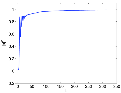
Figure 1: Typical evolution of $\left|\phi\right|^{2}$

If the average field were not close to zero in the initial conditions distribute we would have found that the biased initial conditions would give a different time dependence in the area density Coulson:1996nv ; Larsson:1997sp . Indeed, if one phase is selected in the initial distribution then the evolution of the domain wall area density can be shown to follow the relation

$$A\propto\frac{1}{t}e^{-ct},$$ (10)

where $c$ a positive real number. Percolation theory predicts that for a phase occupying a fraction less than a critical value $p_{c},$ the infinite wall disappears. The dominant phase takes over at a characteristic time scale, and quickly fills the entire simulation volume. In our case $p\simeq 0.5\pm 10^{-7},$ far above the percolation threshold which for a cubic lattice can be shown to be $p_{c}=0.31.$

III.3 Beginning the Evolution

In the beginning of the simulation dissipation is imposed in order for the field to sink in a controlled manner into the minima and to remove spurious high frequency modes. This is controlled by the parameter $\eta$ in (7). The dissipation aids the formation of the domain wall network and as soon as this is formed, dissipation is turned off and the system is left to evolve freely. A small amount of time, roughly the system’s characteristic time, is required for the field to adjust itself into the new equation with no dissipation and continue to evolve. For that reason any regression on data starts a few timesteps after the end of the dissipated period. Turning the dissipation off slowly seems to help the system adjust more quickly to the new conditions and smooths out the effects of this ‘adjustment’ period. More specifically, the end of the dissipation period $T_{D}$ and the beginning of the regression $T_{R}$ are specified in the program and their difference $T_{R}-T_{D}$ is calculated. As soon as the system reaches $T_{D},$ dissipation at timestep $n$ $\eta_{n}$ is decreased till zero using a Gaussian like function

$$\eta_{n}=\eta_{\rm i}\times\exp\left(\frac{-A\left(n-T_{D}\right)^{2}}{\left(T_{R}-T_{D}\right)^{2}}\right)\times\Theta(T_{R}-T_{D}),$$ (11)

where $n$ is the timestep, $\eta_{\rm i}$ the initial dissipation and $A$ a real positive number controlling in more accuracy the length of this period.

Dissipations ranged from 0.1 to 0.3 in the simulations and affected the system for roughly 10%-30% of the total simulation time $T_{tot},$ with regression on the results starting at 20%-40% of the total time and the coefficient $A$ was taken to be in the range $1$ to $1.5$ .

III.4 Wall Area Density Calculation

The main purpose of the simulations was to check the power law for the evolution of the wall area density. A crude way of calculating the total wall area is counting the places where adjacent lattice points have opposite signs and multiplying by $\Delta x$ or $\Delta x^{2}$ which is a rough estimation of the wall area at the “link”. More precisely, one should find an accurate discretization of the continuum area density operator (5).

The calculation is made by finding two adjacent lattice points where the field has opposite signs and calculating the gradient of the field at the “link”. For two such adjacent points $\left\{i,j,k\right\}$ and $\left\{i-1,j,k\right\}$ the gradient is calculated as follows. The numerical approximation to the gradient at the direction of the link is just

$$\Delta_{i}\phi=\frac{\phi_{i,j,k}-\phi_{i-1,j,k}}{\Delta x}$$

whereas the gradients at the remaining two directions are taken by averaging over the gradients of nearby links; the $j$ -component of the gradient for example would be

$$\Delta_{j}\phi=\frac{1}{2}\left(\frac{\phi_{i-1,j+1,k}-\phi_{i-1,j-1,k}}{2\Delta x}+\frac{\phi_{i,j+1,k}-\phi_{i,j-1,k}}{2\Delta x}\right).$$

One needs to account for the orientation of the area element at each link, otherwise one will end up overestimating the area Ryden:1989vj ; Scherrer:1998sq . For domain walls in 3D the problem can be resolved by simply multiplying the lattice area estimate by a factor $\frac{2}{3}$ Scherrer:1998sq , while a similar argument to that given in Scherrer:1998sq gives the factor $\pi/4$ in 2D:

$$A = A_{Lat}\frac{2}{3}\qquad\textrm{(3D)}$$ (12)

$$A = A_{Lat}\frac{\pi}{4}\qquad\textrm{(2D)}$$ (13)

The Figures show $A_{Lat}$, while the Tables show $A$.

IV Results

IV.1 Wall area density

In all simulations the wall area data started to be taken shortly after the dissipation had been stopped. Fig. 2 shows the results from a 2D run, fitted to a

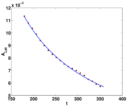
Figure 2: Evolution of the wall area density $A_{Lat}$ for a 2D simulation, $N=1024$, $\Delta x=0.3$, $\Delta t=0.1$.

power law

$$A_{Lat}=at^{-b}$$ (14)

by regression. Five simulations for the same parameters were run and an average was taken, with the fit taken on the averaged area. The results for 2D and 3D simulations are presented in Tables 1, 2, for Minkowski,

Background	Length scaling law
Minkowski	$0.765(0.227).t^{-0.987(0.032)}$
Radiation	$0.928(0.165).t^{-0.996(0.018)}$
Matter	$1.145(0.227).t^{-0.992(0.014)}$

Table 1: Area scaling laws for Minkowski, radiation-dominated, and matter-dominated FRW backgrounds in 2 dimensions. The results are derived from averaging over 5 simulations for each case, with ${\Delta x}=0.3$, ${\Delta t}={0.1}$ and a $1024^{2}$ lattice.

Background	Area scaling law
Minkowski	$0.883(0.141).t^{-0.995(0.026)}$
Radiation	$0.925(0.125).t^{-0.994(0.013)}$
Matter	$0.963(0.122).t^{-0.997(0.012)}$

Table 2: Area scaling laws for Minkowski, radiation-dominated, and matter-dominated FRW backgrounds in 3 dimensions. The results are derived from averaging over 5 simulations for each case, with ${\Delta x}=0.3$, ${\Delta t}={0.1}$ and a $512^{3}$ lattice.

radiation and matter-dominated Friedmann-Robertson-Walker backgrounds respectively. The biggest 3D simulation ($N=4096$, $\Delta x=0.3$, $\Delta t=0.08$) gave $a=0.980(\pm 0.017)$, $b=0.985(\pm 0.003).$

There is a suggestion from the simulations that the wall area decreases slightly slower than $b=1.$ However, this deviation from the $b=1$ scaling could not be attributed to a relation of the form given in Eq. 8, as it has been suggested Press:1989yh . Plotting $\exp(A_{Lat})\times t$ against time shows that there seems to be no logarithmic term in the wall area evolution, Fig. 3.

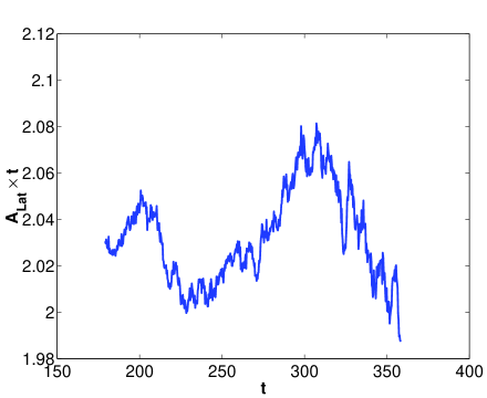
Figure 3: $\exp(A_{Lat}t)$ against time for the simulation of Fig. 2. A decay law $A_{Lat}\sim\log(t)/t$ would show as a logarithmic increase on this graph.

Both the power law and the coefficient $a$ of Eq.  14. present challenges to the analytic method for the calculation of the wall area density of Ref. Hindmarsh:1996xv , which are compared in detail in Hin02 . The power law is very close to the predicted value of $b=1$, with good precision, but the coefficient $a$ showed larger fluctuations between runs.

V Conclusions

The numerical integration of the equations of motion for the the $\phi^{4}$ model has given an insight to the dynamics involved in domain wall networks and has provided an accurate way to support the scaling solution predicted by theoretical computations. A power law with exponent very close to 1 was found to be the best solution according to the simulation data with no evidence for a logarithmic term suggested in previous studies Press:1989yh .

The fact that a domain wall network shows this dynamic scaling over approximately three orders of magnitude in the parameter $M\xi$, the ratio between the local curvature radius and the wall width, is remarkable, and has important implications for cosmic string networks. Firstly, it is clear from the visualisations in Fig. 4 (see also Sims )

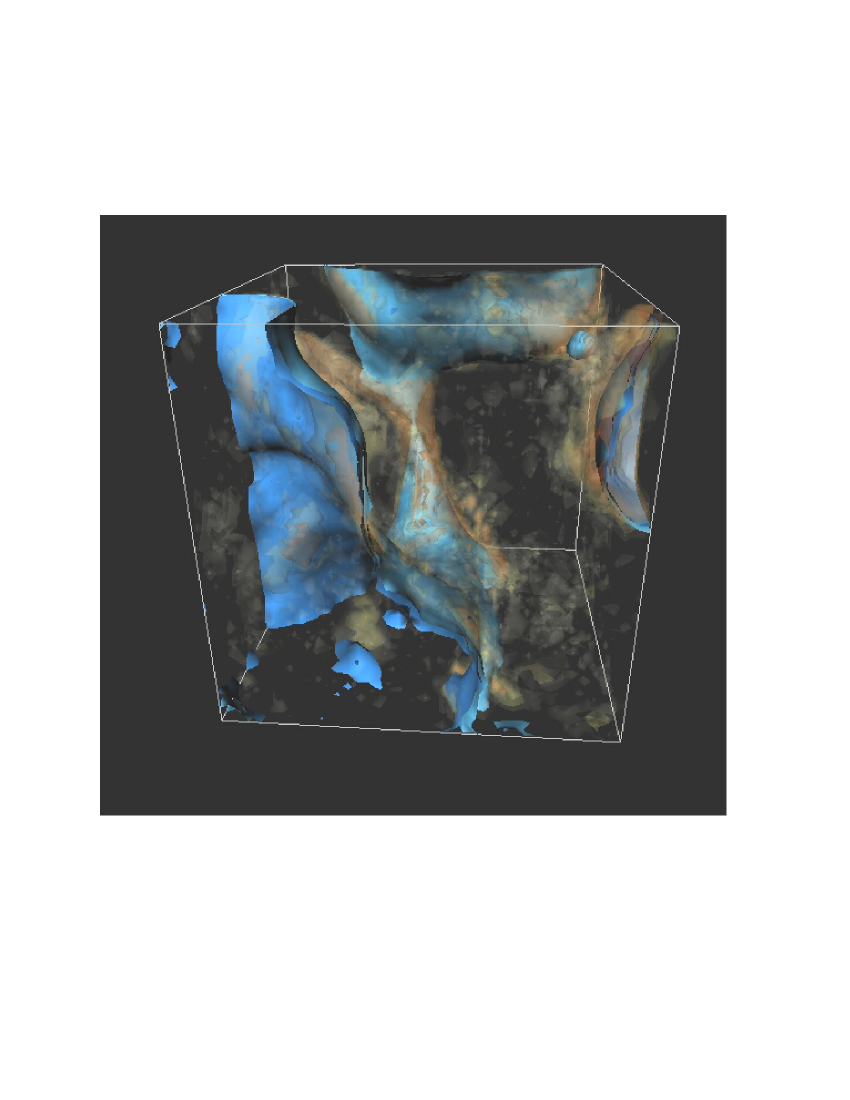
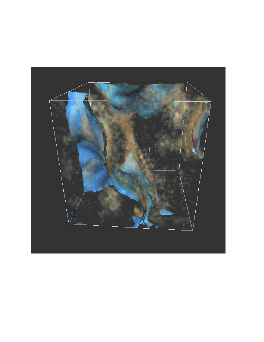
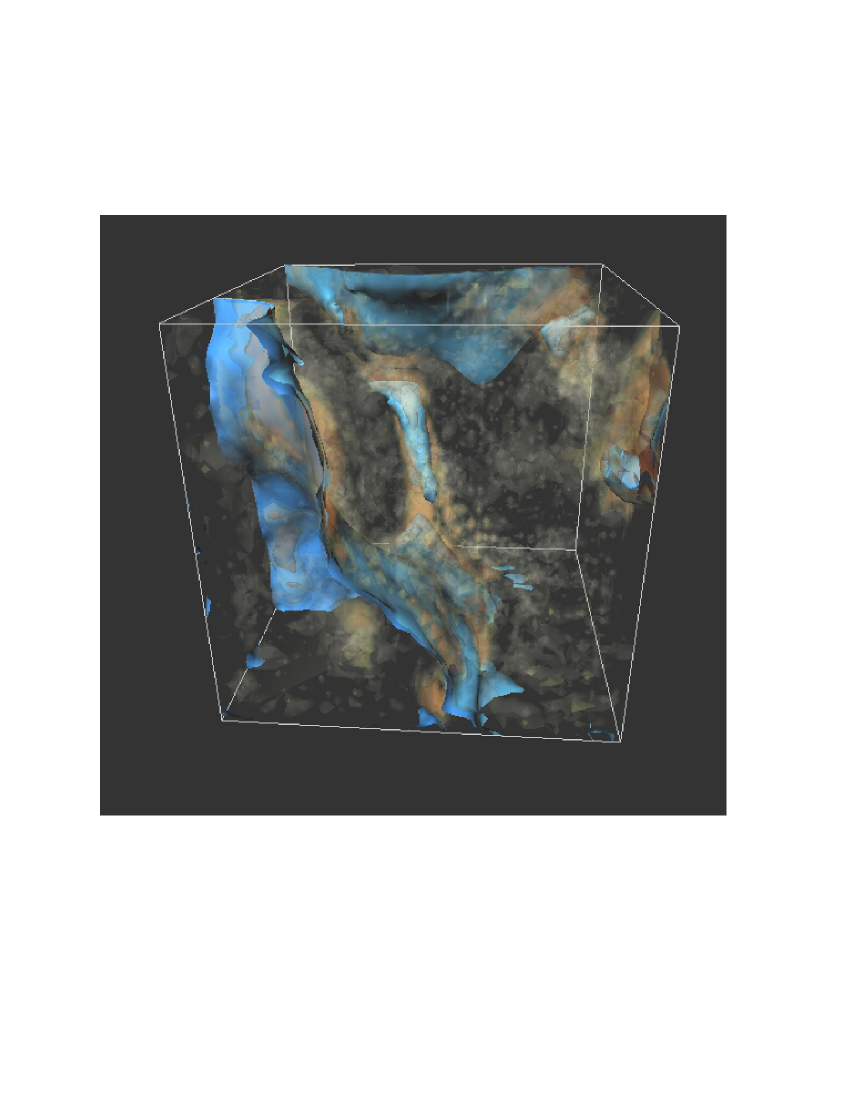
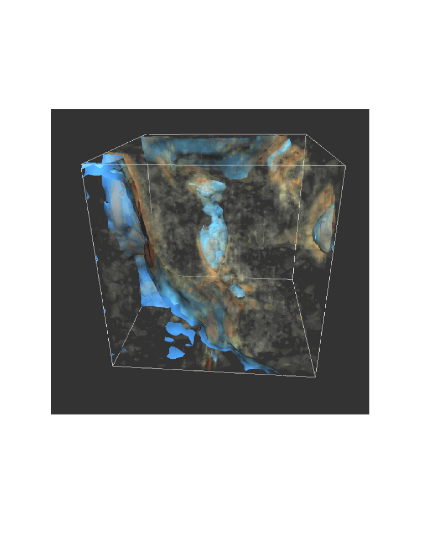
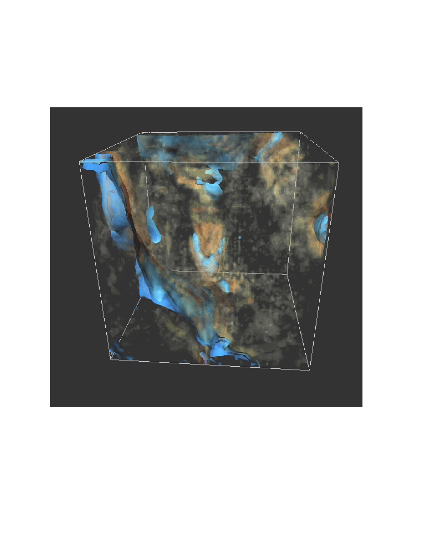
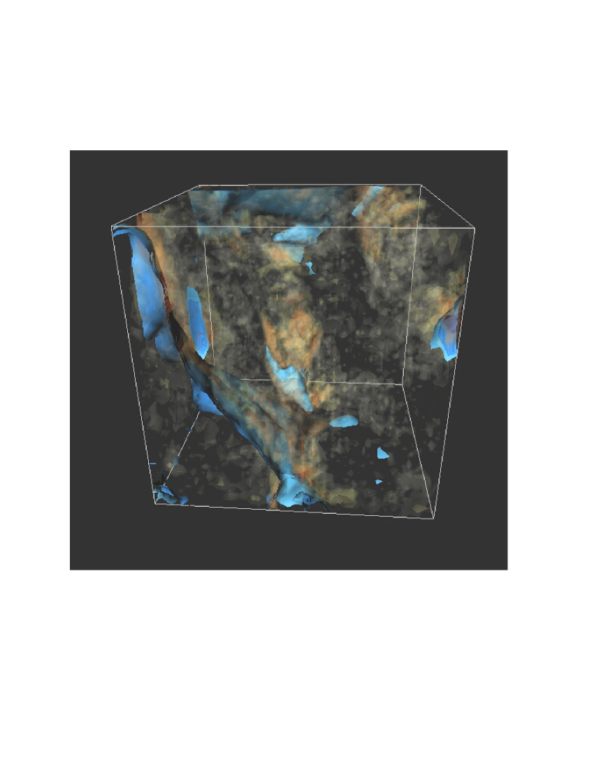
Figure 4: Six snapshots from a numerical simulation using the algorithm described in Sec. III, with time increasing left to right and top to bottom. The solid isosurfaces are surfaces of constant $\phi$, with the red representing small positive values and the blue small negative values. Semi-transparent isosurfaces are surfaces of constant momentum density.

that the energy in the domain walls is very quickly transferred into propagating modes of the field: the formation and collapse of closed loops (2D) or surfaces (3D), expected in the standard picture of the evolution of wall networks VilShe94 , is rare. Indeed, in 2D, self-intersections to form closed loops must be very rare; if two segments of wall approach each other they must be generically curved away from the point of closest approach, and therefore the acceleration is in the direction which would tend to increase the separation. Nonetheless, 2D walls scale perfectly well, so it seems plausible in that case that energy is being transferred directly into radiation. If the amplitude of the oscillations is large enough they could appear to form tiny loops or “protoloops” Moore:1998gp ; Moore:2001px .

We believe that our results add weight to the contention, first put forward in Vincent:1998cx , that extended defects (including cosmic strings in 3D) have a non-perturbative channel into massive radiation. At first sight this is difficult to square with the standard picture, in which walls and strings obey the Nambu-Goto equations of motion for large curvature radii, for in that case the total energy locked up in the extended defects is conserved, in the absence of an general relativistic effects such as an expanding background or gravitational radiation. It is certainly true that it is possible to find string trajectories which are very close to being solutions of the Nambu-Goto equations Moore:1998gp ; Olum:2000sg : however, the initial conditions have to be carefully prepared, and the existence of these trajectories does not preclude the existence of a non-perturbative radiative process for defect networks. Indeed, we maintain that our results are good evidence that there must be such a process.

Appendix A Lattice Correction factor for 2D wall length density

In Ref. Scherrer:1998sq it was shown that the naive lattice estimate of the area density of random domain walls in 3D overcounts the continuum value by a factor of 3/2 in the limit that the radii of curvature are large compared with the lattice spacing. In this section we perform the analagous calculation for two dimensions, finding it to be $4/\pi$.

The naive estimate is obtained by summing the length of all links containing a wall and dividing by the total volume. A link crossing a wall is defined to be one for which the values of the field $\phi$ on the sites at either end have opposite signs. One can immediately see this will overestimate the length, as one is approximating a smooth curve by a sequence of line segments parallel to the lattice vectors ${\mathbf{i}}$ and ${\mathbf{j}}$.

In the continuum the centre of a domain wall is described by a 2-dimensional curve ${\mathbf{r}}(\sigma)$. Consider a segment of length $l$, with $l\ll\xi$, where $\xi$ is the correlation length of the curve. Writing $\Delta{\mathbf{r}}={\mathbf{r}}(l)-{\mathbf{r}}(0)=x{\mathbf{i}}+y{\mathbf{j}}$, we see that the lattice approximation to the length is

$$l_{\mathrm{Lat}}=|x|+|y|.$$ (15)

In the limit that $l/\xi\to 0$, the continuum value of the length is $l=\surd(x^{2}+y^{2})$. Hence

$$l_{\mathrm{Lat}}=\frac{l_{\mathrm{Lat}}}{l}l=(|\cos\alpha|+|\sin\beta|)l$$ (16)

where $\alpha$ and $\beta=\pi/2-\alpha$ are the direction cosines of the vector $\Delta{\mathbf{r}}$. The ratio between the lattice estimate of the length and the true length is obtained by averaging over all possible orientations of the lattice relative to $\Delta{\mathbf{r}}$:

$$\left\langle\frac{l_{\mathrm{Lat}}}{l}\right\rangle=\frac{1}{2\pi}\int_{0}^{2\pi}d\alpha\left(|\cos\alpha|+|\sin\alpha|\right)=\frac{4}{\pi},$$ (17)

as advertised.

This calculation can be extended to arbitrary $l$ through a more involved argument. Let us first define the correlation function

$$C(r)=\langle\phi({\mathbf{r}})\phi(0)\rangle,$$ (18)

which is assumed to be smooth at ${\mathbf{r}}=0$, so that

$$C(r)=C(0)-\frac{1}{2}C^{\prime\prime}(0)r^{2}.$$ (19)

In Refs. OhtJasKaw82 ; Hindmarsh:1996xv it is shown that the length density $A$ of the locus of zeroes of a Gaussian random field in 2 dimensions is given by

$$A=\frac{1}{2}\sqrt{-\frac{C^{\prime\prime}(0)}{C(0)}}.$$ (20)

This is the value of the length density in the continuum.

On the lattice, we must consider the probability that the values of the field at opposite ends of a link have opposite signs, in which case we can say that the link is occupied by a segment of domain wall. Let us call this probability $p_{\mathrm{occ}}$, which is

$$p_{\mathrm{occ}}=2P(\phi({\mathbf{x}})>0\;\mathrm{AND}\;\phi({\mathbf{x}}+{\mathbf{i}}\Delta x)<0),$$ (21)

where the factor of 2 accounts for the opposite case $\phi({\mathbf{x}})>0\;\mathrm{AND}\;\phi({\mathbf{x}}+{\mathbf{i}}\Delta x)<0$. The lattice estimate of the length density is then

$$A_{\mathrm{Lat}}=\frac{2p_{\mathrm{occ}}}{\Delta x},$$ (22)

where the lattice spacing is $\Delta x$, and the factor 2 comes from the fact that there are twice as many links as sites in 2 dimensions.

Suppose we now define

$$P_{12}(C(r_{12}),V)=P(\phi({\mathbf{x}}_{1})>V\;\mathrm{AND}\;\phi({\mathbf{x}}_{2})<V),$$ (23)

where $V$ is an arbitrary threshold and $r_{12}=|{\mathbf{x}}_{1}-{\mathbf{x}}_{2}|$. One can then almost trivially write

$$P_{12}(C(r_{12}),V)=\int_{0}^{r_{12}}\frac{\partial P_{12}}{\partial C(r)}\frac{dC(r)}{dr}dr.$$ (24)

It can be shown HamGotWei86 that

$$\frac{\partial P_{12}}{\partial C_{12}}=\frac{1}{2\pi[C(0)^{2}-C_{12}^{2}]^{\frac{1}{2}}}\exp\left(-\frac{V^{2}}{C(0)+C_{12}}\right),$$ (25)

where $C_{12}=C(r_{12})$. Hence the lattice estimate of the area density is

$$A_{\mathrm{Lat}}=\frac{2}{\pi\Delta x}\cos^{-1}\left(\frac{C(\Delta x)}{C(0)}\right).$$ (26)

Providing $\Delta x$ is much smaller than the correlation length $\xi$, defined by $\xi^{2}=|C(0)/C^{\prime\prime}(0)|$, we see that

$$A_{\mathrm{Lat}}=\frac{2}{\pi}\sqrt{-\frac{C^{\prime\prime}(0)}{C(0)}},$$ (27)

and hence, from Eq. (20), that $A_{\mathrm{Lat}}=4A/\pi$.

References

- (1) D. A. Kirzhnits, JETP Lett. 15, 529 (1972).
- (2) L. Dolan and R. Jackiw, Phys. Rev. D 9, 3320 (1974).
- (3) D. A. Kirzhnits and A. D. Linde, Annals Phys. 101, 195 (1976).
- (4) Y. B. Zeldovich, I. Y. Kobzarev and L. B. Okun, Zh. Eksp. Teor. Fiz. 67, 3 (1974).
- (5) T. W. Kibble, J. Phys. A A9, 1387 (1976).
- (6) Y. B. Zeldovich, Mon. Not. Roy. Astron. Soc. 192, 663 (1980).
- (7) A. Vilenkin and Q. Shafi, Phys. Rev. Lett. 51, 1716 (1983).
- (8) A. Vilenkin, E.P.S. Shellard Cosmic Strings and other Topological Defects (Cambridge University Press 1994)
- (9) M. B. Hindmarsh and T. W. Kibble, Rept. Prog. Phys. 58, 477 (1995) [hep-ph/9411342].
- (10) D. Austin, E. J. Copeland and T. W. Kibble, Phys. Rev. D51, 2499 (1995) [hep-ph/9406379].
- (11) W. H. Press, B. S. Ryden and D. N. Spergel, Astrophys. J. 347, 590 (1990).
- (12) D. Coulson, Z. Lalak and B. Ovrut, Phys. Rev. D53, 4237 (1996).
- (13) S. E. Larsson, S. Sarkar and P. L. White, Phys. Rev. D55, 5129 (1997) [hep-ph/9608319].
- (14) G. Vincent, N. D. Antunes and M. Hindmarsh, Phys. Rev. Lett. 80, 2277 (1998) [hep-ph/9708427].
- (15) J. N. Moore and E. P. Shellard, [arXiv:hep-ph/9808336].
- (16) J. N. Moore, E. P. Shellard and C. J. Martins, [arXiv:hep-ph/0107171].
- (17) B. S. Ryden, W. H. Press and D. N. Spergel, Astrophys. J. 357, 293 (1990).
- (18) M. Yamaguchi, J. Yokoyama and M. Kawasaki, Phys. Rev. D61, 061301 (2000) [hep-ph/9910352].
- (19) D. P. Bennett and S. H. Rhie, Astrophys. J. 406, L7 (1993) [hep-ph/9207244].
- (20) M. Yamaguchi, Phys. Rev. D 64, 081301 (2001) [arXiv:hep-ph/0103130].
- (21) M. Yamaguchi, arXiv:hep-ph/0107230.
- (22) R. Durrer, A. Howard and Z. Zhou, Phys. Rev. D49, 681 (1994) [astro-ph/9311040].
- (23) U. Pen, D. N. Spergel and N. Turok, Phys. Rev. D49, 692 (1994).
- (24) T. Ohta, D. Jasnow, and K. Kawasaki, Phys. Rev. Lett. 49, 1223 (1982).
- (25) M. Hindmarsh, Phys. Rev. Lett. 77, 4495 (1996) [hep-ph/9605332].
- (26) M. Hindmarsh and E.J. Copeland “Defects without Computers” in ‘Topological defects in Cosmology’, eds F. Melchiorri and M. Signore, (World Scientific, Singapore, 1997).
- (27) M. Hindmarsh “Dynamics of Defect and Brane Networks” [arXiv:hep-ph/0207267].
- (28) W. H. Zurek, Phys. Rept. 276, 177 (1996) [aarXiv:cond-mat/9607135].
- (29) R. J. Scherrer and A. Vilenkin, Phys. Rev. D58, 103501 (1998) [hep-ph/9709498].
- (30) Animation and images of the simulations can be found on our website at http://www.pact.cpes.susx.ac.uk/arXiv/0212350/
- (31) K. D. Olum and J. J. Blanco-Pillado, Phys. Rev. Lett. 84, 4288 (2000) [astro-ph/9910354].
- (32) A.S. Hamilton, J.R. Gott and D. Weinberg, Ap. J. 309, 1 (1986).