Evidence of Non-Zero Mass Features for the Neutrinos Emitted at Supernova LMC-’87A

Abstract

The observation of the neutrinos arrived from Supernova LMC-’87A shows, with a good confidence level, the existence of two massive neutrinos. For the unobserved third neutrino mass, could speculate two possibilities either that this mass is close to one of the two observed values or that this neutrino has a negligible electronic flavor component.

1 Introduction

The explosion of a faraway supernova is an event quite suitable for understanding some of the most important physical features of neutrinos. After being produced, neutrinos pass through dense matter and therefore both their initial flavors and masses might considerably change. However, in their subsequent long journey through a good vacuum towards the Earth, no further interaction will practically occur, and their mass states will not change. If the masses of the three kinds of neutrinos are not zero and differ from each other more than order of eV, the wave packet of each mass state will separate from the others much more than the Earth dimension and there would be almost no interference between states of different masses. The detector can see all the three flavors for each separate mass group provided the neutrino energy is high enough. Therefore a complete knowledge of the basic features of neutrinos, i.e. the mass values and the mixing angles to all the flavor states from each separated mass state, could be obtained without too big uncertainty.

The explosion of Supernova LMC-’87A has been a lucky event, since it occurred at a distance of $\sim$ 200,000 light-years and the produced neutrinos arrived on the Earth in 1987, when three huge detectors, able to observe neutrino interactions, were already operative. Moreover, the distance is large enough to separate the neutrino mass states (provided these differ more than order of eV) and, at the same time, is not so large to make the statistics of the observed events too poor for a quantitative analysis.

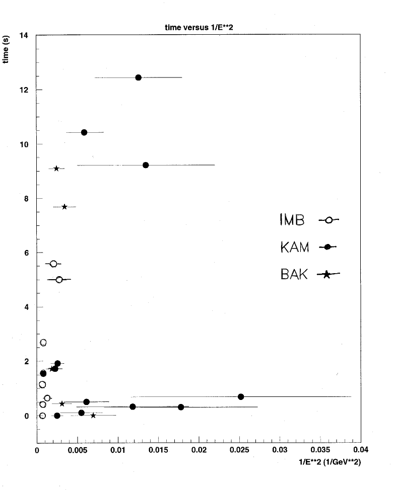
Figure 3: T vs. $1/E^{2}$ Plot of the observed events

The observations made at Kamiokande II [1, 2], IMB [3, 4] and Baksam [5] show an apparent disagreement with the theory: the number of the observed events is roughly one order of magnitude smaller, while the spread in the arrival times is about one order of magnitude larger than the values, both comparing to the values expected on a theoretical ground [6]. Thus, the first disagreement indicates an explosion smaller than the predicted one, while the second indicates a bigger. This contradiction disappears if neutrinos are massive particles. In this case, a massive neutrino with a lower energy travels more slowly than a higher energy one and will arrive on the Earth appreciably later than the latter due to long distance the neutrinos must go through. In this way, the large spread observed in the arrival times could be easily understood. A further consequence of the assumption that neutrinos are massive particles is the fact that the plot of the arrival time of each neutrino versus the reciprocal of the square of the observed energy must show a grouping of the points along three different straight lines, whose slopes are proportional to the squared mass of each kind of neutrino (see sect. 5). The plot is given in Fig.3. It shows only two linear groupings indicating the mass values $3.4\pm 0.6$ and $22.7\pm 3.7$ eV. One could speculate on the reasons hiding the third mass value (or the third linear grouping). This mass could be close to one of the two observed mass values or the electronic flavor of the third neutrino could be so small to yield visible events. In the latter case its mass value is completely unknown and any positive value, including zero, is possible.

2 Discrepancy between expectation and observation by Kamiokande II

Due to the fact that the neutrinos arriving from Supernova LMC-’87A do not have a very high energy, their observation was made possible by detecting the electrons produced by the neutrino charged current interactions in the detector. The observed electron energy gives a good estimate of the primary neutrino energy while the neutrinos’ arrival times are measured with a precision higher than a millisecond. Therefore we have two well observed quantities for each event: the neutrino energy and the arrival time.

According to theoretical predictions, the Kamiokande II detector in Japan (3 kilo tons of water) should have observed, within a few seconds or less, nearly 50 events with energy higher than 10 MeV, with an average energy of $10\sim 15$ MeV. The real events observed at Kamiokande II were in total 12 with an average energy of 14.6 MeV, and only 7 of these had an energy higher than 10 MeV. Further, the total time spread between the first and the last observed events was found to be equal to 12.44 seconds.

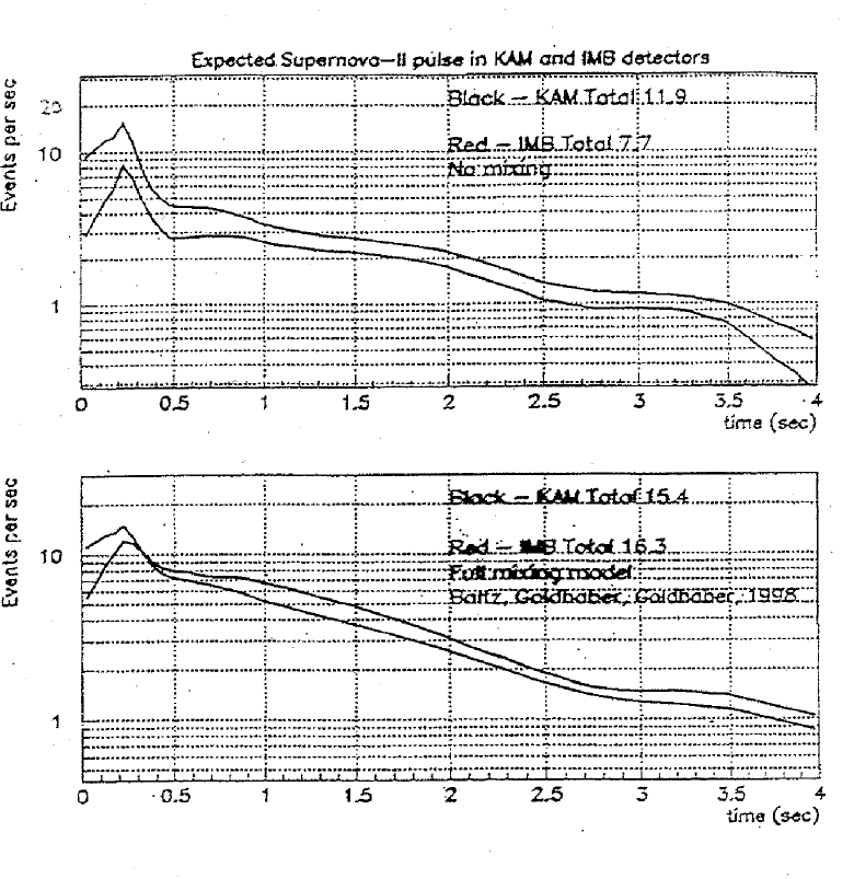
Figure 1: Expected Time Distribution of Neutrinos produced at LMC’87-A

Considering the lowest energy value (6.3 MeV) of the observed events as the detector’s threshold energy and the fact that around this energy the detector efficiency is still rather low, the real average energy should be lower than 14.6 MeV. It could likely be about 10 MeV, or even lower. The observed small number of events with energy greater than 10 MeV, where the detector’s efficiency should already be fairly good, indicates that the real supernova explosion was energetically less powerful than theoretically expected. On the contrary, the wide time spread of the observed events appears to indicate that the real explosion was much bigger, so as to have a longer emission of neutrinos. In fact, according to estimations, the majority of events were expected to occur within one second and only a negligible fraction was expected after a few of seconds (see Fig.1) [9].

The two discrepancies between the observed and predicted number of events and the observed and predicted spread of their arrival times appear to be contradictory. But, as already anticipated, this inconsistency is only apparent since it reflects the fact that neutrinos are massive particles, as it will appear clear in the following. In fact, while massless neutrinos propagate with the light speed and their time distribution does not change whatever the distance they go through, for massive neutrinos the time spread in the arrival times does no longer depend only on the spread in their production times but also on the time delay for traveling the distance Supernova-Earth. Thus, for each neutrino, this arrival time depends both on its mass and its energy, since the velocity of a massive particle depends on these two quantities.

3 Comparison of the Kamiokande data with that of the IMB and the Baksam

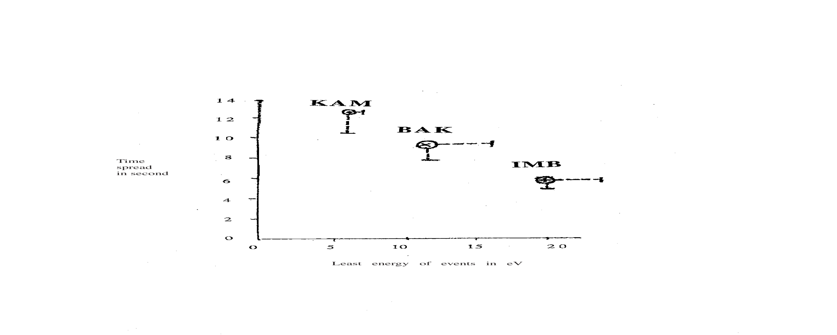
Figure 2: Relation between the lowest energy of events and the spread of arriving time of events

The Kamiokande II data can be compared with those observed by the IMB detector in USA and the Baksan detector in Caucasus, which have different threshold energies, because the time distribution of events does neither depend on the detectors’ working mechanism nor on their dimensions, responsible only of their statistical efficiency. The correlation between the spread time (i.e. the time difference between the first and the last arrived events) and the lowest energy of the observed events (related to the detector’s threshold) is shown in the following table and in Fig.2.

		The lowest energy(MeV)		Spread time (s)
Kamiokande II		6.3		12.4
Baksan		12.0		9.1
IMB		20.0		5.6

In Fig.2, for each detector the error bars were obtained using the differences between the observed lowest energy values and between the observed latest arrival times, respectively. The figure shows that the observed time spreads depend almost linearly on the threshold energies of the detectors.

Even if the neutrinos with lower energies were produced at the tail of the explosion interval, this fact could not explain such a big difference in the time spread due to the sharp fall off of events. The spread of the arrival times in the IMB detector, which cannot observe neutrino energy lower than 20 MeV, is nearly 6 seconds, nearly half of the value observed at Kamiokande II, but still much longer than the expected duration of the supernova explosion. Furthermore, in spite of its lower statistics, the Baksan data, collected with a threshold energy about halfway between the IMB and the Kamiokande II ones, give a time spread about halfway between the values obtained by the last two laboratories.

In the next sections, it will be shown that also this smooth change of the time spreads with the detectors’ thresholds is an effect related to the non-zero masses of the neutrinos arriving on the Earth.

4 Time delay of massive neutrino

Let us look now at the time delay in the arrival time of a non-zero mass neutrino in comparison to that of a massless one. If the mass is exactly zero, the time of flight for arriving on the Earth from the Supernova is the same for all the neutrinos. It is

$$T_{0}=L_{SN}/c=1.7\cdot 10^{5}\quad years$$

where $L_{SN}$ is the distance of the Supernova from the Earth, and c is the light speed in vacuum. However if the mass m is not zero, then the time of flight is

$$T_{m}=\frac{L_{SN}}{c\cdot\sqrt{1-(m/E)^{2}}}\sim\frac{L_{SN}}{c}\cdot\{1+\ 1/2\cdot(m/E)^{2}\}$$

The difference of these two values, i.e. the delay in the arrival of a neutrino with mass m in comparison to a massless one, is

$$\Delta T_{m}=T_{m}-T_{0}\approx 1/2\cdot T_{0}\cdot m^{2}/E^{2}$$

Numerically, a neutrino of energy 5 MeV should delay about one second if the mass is 3 eV and about 10 seconds if the mass is 10 eV.

5 Data plotted in the diagram: $\Delta T$ vs. $1/E^{2}$

The best way to see if such a mass effect exists at all consists in plotting $\Delta T$, the arrival time delay of each event, versus $1/E^{2}$, the reciprocal of the observed squared energy. Before doing that, it is noted that the supernova explosion takes a finite (non zero) time. Thus the delay in the arrival time of the nth observed event reads

$$\Delta T_{n}=\tau_{n}+T_{0}m_{\alpha}^{2}/2E_{n}^{2},$$

where index $\alpha$ specifies the kind of the arrived neutrino and $\tau_{n}$ denotes the time when the neutrino was produced since the start of the supernova explosion. It should be observed that $\Delta T_{n}$ increases with n and that it depends on the observed energy $E_{n}$ as well as on the mass - for the moment unknown - of the n th observed neutrino. Assuming that the distribution of the emission time $\tau_{n}$ is narrow, from the previous equation it follows that, in a diagram $\Delta T$ versus $1/E^{2}$, the data points ($\Delta T_{n},1/E_{n}^{2}$) should clearly form a straight line with a positive and finite slope, if the neutrinos have a non-zero mass. In fact, the slope is simply proportional to the squared mass value of the neutrino. Moreover, if there are more than one mass state, in the diagram one should observe as many straight lines as the number of the different masses not equal to zero. If the supernova explosion takes a finite time, then the points ($\Delta T_{n},1/E_{n}^{2}$), relevant to neutrinos with mass $m_{\alpha}$, must lie inside a stripe delimited by two parallel straight lines with slope equal to $T_{0}m_{\alpha}^{2}/2$. Noting that the $\tau_{n}$ distribution is the same for each mass group, because the explosion is the same for each mass state, and the intersection of each stripe with the time axis will also be the same.

In Fig.3 we report all the data observed by the three laboratories mentioned above. This procedure is quite legitimate. In fact, the different location of the laboratories on the Earth is at most responsible for a delay of a tenth of second, while the uncertainty in the time zero among the different detectors can be estimated in less than 2 tenths of second from the time separation in the arrival times of the first events at each detector. (Of course, these two uncertainties disappear if we confine ourselves to consider the data collected by a single laboratory.) It should be also noted that Fig.3 was obtained by setting the origin of the time axis at the arrival time delay of the first observed event. As a consequence of this choice, assuming the explosion instantaneous, each straight line will intersect the time axis slightly before the origin. Fig.3 clearly shows two well separated grouping of the observed events. Moreover, each group obeys the conditions required by the massive nature of neutrinos, namely:

1) a less energetic event arrives later than a more energetic one within experimental errors,

2) the events are well distributed inside a narrow strip close to a straight line,

3) the slope of this line is positive and is proportional to the squared mass of the corresponding neutrino,

4) the straight line intersects the time axis just before the arriving time delay of the first event,

5) the linear course grained distributions of the points inside each strip are similar for the two strips, and the intersections of the strip with the time axis are roughly less than 1 s.

The linear fits of the two grouping of the only Kamiokande II data, characterized by a lower energy threshold and a lower experimental error, yield the following two mass values [10]

$$m_{1}=3.4\pm 0.6eV$$

and

$$m_{2}=22.\pm 4.eV$$

The data plot in this diagram two separated linear mass groups are very clearly visible. The order statistics applied to the relation between order of arriving time and that of its energy of the events, for the first and the second mass group separately, gives us both more than 90% confidence. However this statistics tests only monotone relation between two orders without discriminating two opposite sense of relations; in our case, physically good sense or nonsense (lower energy event arrives later or earlier). Adding this effect the above obtained value becomes as more than 95%. Furthermore taking into account the other physically necessary conditions; 1) not only monotonous relation in good sense but also the linear form in this diagram, further 2) the fact that this line should hit a little bit before the arriving time of the first event, and also 3) the consistency with all the other data obtained by independent apparatus, the confidence level should be very high.

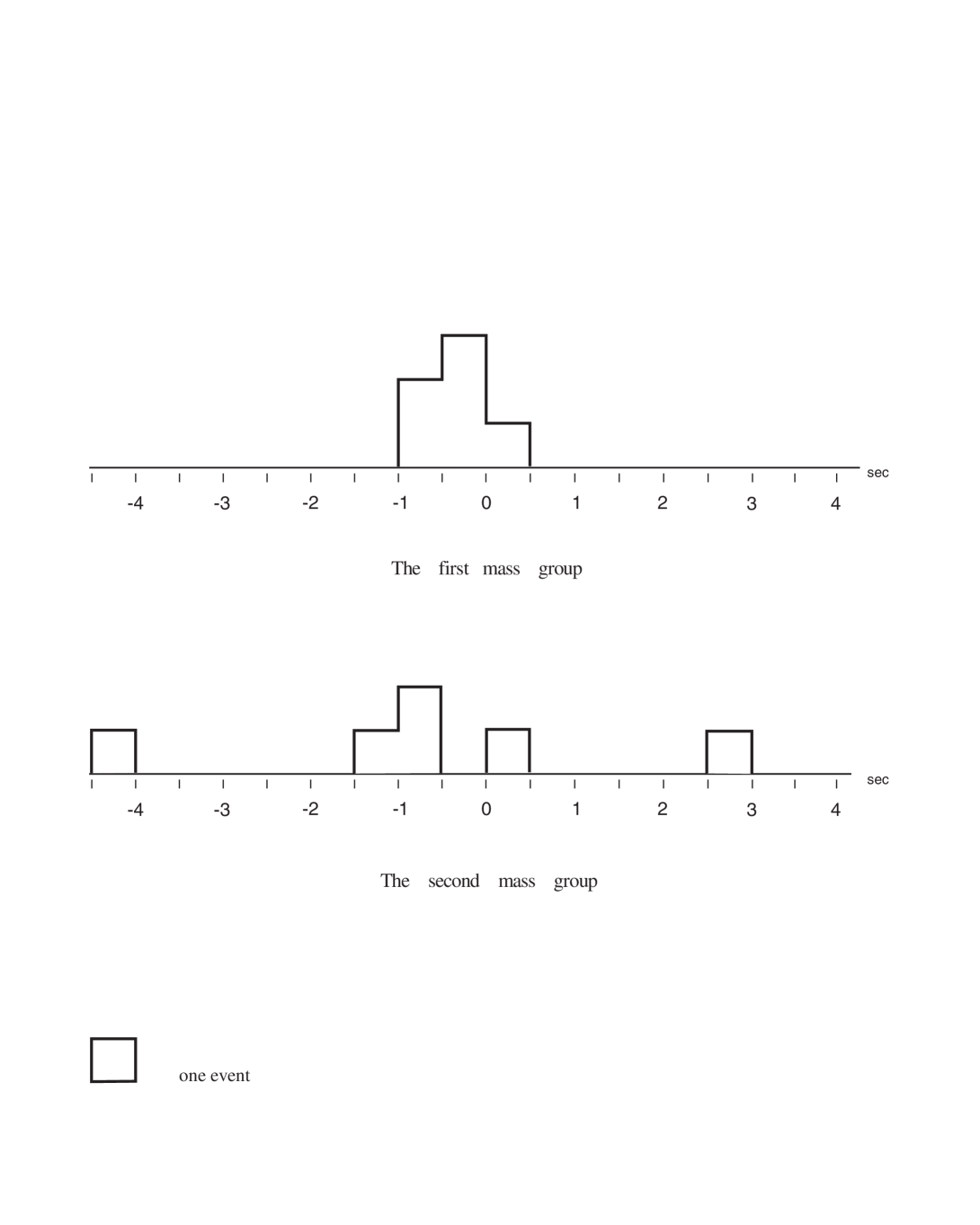
Figure 4: Emission time distribution of neutrinos at the Supernova

Very rough time distribution of the neutrino emission at the Supernova can be easily obtained and shown in Fig.4 both $m_{1}$ and $m_{2}$ separately. The distribution for $m_{2}$ comes out very much wider. But two events far from the center of the explosion corresponding to a little before the time zero, one at about the beginning and the other twards the ending, have the time errors of several seconds due to the large observation error of low energy and also due to the large slope of the mass-fit line. Both events are the last arriving in the detector of KAM II. Taking into account this effect, the both emission time distribution are consistent as the same.

6 Discussion

The previous plot and the mass values obtained by its analysis deserve some remarks:

1) It should be noted the usefulness of plotting the delay in the arrival times of neutrinos versus the reciprocal squared energy. It is this plot that clearly shows the separation of the observed events into two groups. The precise determination of the arrival times and the $10\sim 30$% errors on the energies of the observed neutrinos allows us to fit the separate groups of events with two straight half lines which intersect the vertical axis near the origin. In this respect, the assumption that neutrinos are massive particles plays the fundamental role. On the one hand, it explains the separate groupings of the events. On the other hand, it also explains the rather large spread in the arrival times. Moreover, the energy distributions in the two groups of events look similar (see Fig.5 in Ref.[10]).

2) For each group of events, consider now the deviation, along the time axis, of each event from the best-fitted straight line. The distributions of these deviations, that correspond to $\tau_{n}$ of the preceeding section, are also quite similar between the two groups and narrower than one second. The similarity of the distributions of energy and time deviation for the two groups of events is consistent with the fact that the neutrino of each event, produced during the supernova explosion with a well defined flavor state, generates well separated mass states after its long journey towards the Earth. Last but not least, the best fit of the two almost linear groupings allows us to determine the masses of at least two neutrinos (for the third neutrino mass, see the discussion in the next section) and not simply their mass difference.

3) It is important to combine in a single plot all the data collected by the three laboratories. It has already been explained the reason why this is legitimate. We stress now the usefulness of this procedure. The data collected by the IMB apparatus refer to rather energetic neutrinos owing to the high energy threshold of the detector. Thus, no wonder that the IMB data show only one grouping of these events so as to make the observation of two masses impossible. The data collected by the Baksam apparatus refer to neutrinos of lower energy. But, due to the small size of this detector, the total number (only 5) of the detected events is too small to make any mass effect clearly visible. However, this effect becomes clearly visible in the plot including Kamiokande II data. In fact, the Kamiokande II detector performed much better thanks to its larger size and to the enormous efforts made to purify the water of the apparatus so as to ensure a very good transparency to faint light (the Kamioka underground mine has a wonderful water spring that produces excellent pure water in enormous quantity, but this is only a small part of the excellent function of this detector) and it has a much lower energy threshold. In this way, the low-energy events detected by the Kamiokande II apparatus make the separation of the events into two groups quite evident.

4) The previous findings no longer require to assume that the duration of the supernova explosion is longer than predicted in order to explain the wide spread observed in the arrival times, and that a large fraction of low energy neutrinos is produced toward the end of the supernova’s explosion. Furthermore, an explosion of 10 s or more would make it difficult to explain the reason why the observed events lie within two different strips. On the contrary, the small time spread of the two bunches of straight lines in the plot indicates that the explosion lasted less than 1 s. A shorter explosion also agrees with the observation that only 7 events, instead of the expected 50 ones, have energy higher than 10 MeV.

5) The mechanism that could show particle mass in the method is extremely simple and fundamental rule in physics: the relation between velocity and energy of a particle that depends on only one variable, its mass. It is clear that the method does not depend on the initial condition of the particle at leaving from the source, but only on the observation of the particle on the Earth. Also often physical value and character of a particle appears in several different independent modes. In this case each result of all the different mechanism should be physically important.

7 The third mass

Neutrinos are expected to have three mass states as well as three flavors. Then, one rightly wonders why only two mass values are clearly visible in the reported plot. We are therefore obliged to speculate on the possible reason hiding the appearance of a third mass value.

1) If the third mass is zero and it interacts in the electronic flavor channel, it cannot escape from observation. In this case, the associated events should concentrate in a narrow group around the time of the first arrived event. This group cannot experimentally get lost. Thus one concludes that the existence of a massless neutrino with electronic flavor is impossible.

2) If we assume that the third mass is very large, e.g. around 100 eV or bigger, the arrival times of these neutrinos would spread over a time range wide several minutes or more. Then, it would be quite awkward to distinguish the real supernova signals from the background events. However, if the mass is so large, it should easily be observed through decay processes of charged leptons or in neutrino oscillation phenomena. In conclusion, the existence of a quite large mass neutrino appears unlikely.

3) The missing mass state could have a mixing angle of nearly 90 with the electronic flavor state (i.e. a very small component of electronic flavor state). Thus such neutrinos could hardly produce a visible electronic event. Moreover, the highest energy value observed for the neutrinos, arrived from the supernova, is 40 MeV, and energies higher than this value are quite unlikely according to theoretical estimates of the explosion power [1]. Thus, this kind of neutrinos would hardly have enough energy to produce other leptons as a muon (105.66 MeV) or a much heavier tauon (1784.2 MeV) via other flavor channels. Therefore, in this case, any value for the third mass is possible, including the zero value. Besides, if such a case were true, the nearly equal number of events in the two mass groups indicates that these two mass states have roughly the same mixing angles with the electronic flavor state and therefore the maximum mixing would be favored.

4) The mass value of the third neutrino is fairly close to one of the two observed values (within a few of eV). Thus, either

$$m_{3}\approx m_{1}$$

or

$$m_{3}\approx m_{2}$$

The second possibility is favored by the recent results on the atmospheric neutrino oscillations, observed at Super-Kamiokande [11, 12] by comparing the neutrino behaviors over distances of the Earth diameter, since the observed squared mass difference turned out to be about $10^{-3}(eV)^{2}$.

5) It is also mentioned that some theoretical models on neutrino mixing predict only two observable mass states [13].

8 Conclusion

Neutrinos emitted from a very distant supernova, once arrived on Earth, could reveal all their physical features, as masses and mixing angles among both mass- and flavor-states, if all the flavors can be observed by the detectors and if all the three mass states are well separated.

In the case of Supernova LMC-’87A, however, it was impossible to get this full information partly because the only electronic flavor could be observed due to the low energy of neutrinos and partly because two masses only are visibly separated. Even though no information about the mixing angles among mass and flavor states can be obtained, this explosion was an extremely important opportunity to prove the existence of at least two massive neutrino kinds and to get a reliable estimate of their masses. This was made possible by the plot of the time delay in the arrival times versus the reciprocal squared energy of the events. The plot also showed the full consistency of the data observed by the three laboratories. For the third neutrino mass, one can only say either that its value is close to one of the observed ones or that it is not visible because the neutrino has a very small electron flavor.

References

- [1] H. Hirata et al., Phys. Rev. Letters B, Vol. 58 (’87), 1490.
- [2] H. Hirata et al., Phys. Rev. D Vol. 38 (’88), 448.
- [3] R. M. Bionta et al., Phys. Rev. Letters Vol. 58 (87), 1494.
- [4] C. B. Bratton et al., Phys. Rev. D Vol. 37 (’88), 3351.
- [5] E. N. Alexeyev et al., Phys. Rev. Letters B, Vol. 205 (’88), 209.
- [6] J. N. Bahcall, A. Dar and T. Piran, Nature Vol. 326 (’87), 133.
- [7] J. R. Wilson ”Numerical Astrophysics”(1986), Ed.s Centrella J. et al., (Jones & Bartlett, Boston).
- [8] J. R. Wilson et al. N.Y. Acad. Sci. Vol. 470 (’86), 267.
- [9] M. Goldhaber and M. Divanat, Neutrino Telescope. Venice (’99).
- [10] H. Huzita, Modern Physics Letters A, Vol. 2 (’87), 905.
- [11] Y. Fukuda et al., Phys. Rev. Letters, Vol. 82 (’99), 2644.
- [12] Y. Fukuda et al., Phys. Letters B, Vol. 467 (’99), 185.
- [13] S. M. Bilenky, C. Giunti and W. Grimus, Prog. Part. Nucl. Phys. Vol 43 (’99), 1