Electroproduction of Charmonia
off Protons and Nuclei

Abstract

Elastic virtual photoproduction of charmonia on nucleons is calculated in a parameter free way with the light-cone dipole formalism and the same input: factorization in impact parameters, light-cone wave functions for the photons and the charmonia, and the universal phenomenological dipole cross section which is fitted to other data. The charmonium wave functions are calculated with four known realistic potentials, and two models for the dipole cross section are tested. Very good agreement with data for the cross section of charmonium electroproduction is found in a wide range of $s$ and $Q^{2}$. Using the ingredients from those calculations we calculate also exclusive electroproduction of charmonia off nuclei. Here new effects become important, (i) color filtering of the $c\bar{c}$ pair on its trajectory through nuclear matter, (ii) dependence on the finite lifetime of the $c\bar{c}$ fluctuation (coherence length) and (iii) gluon shadowing in a nucleus compared to the one in a nucleon. Total coherent and incoherent cross sections for C, Cu and Pb as functions of $s$ are presented. The results can be tested with future electron-nucleus colliders or in the peripheral collisions of relativistic heavy ions.

1 Introduction

In contrast to hadro-production of charmonia, where the mechanism is still debated, electro(photo)production of charmonia seems better understood: the $c\bar{c}$ fluctuation of the incoming real or virtual photon interacts with the target (proton or nucleus) via the dipole cross section ${\sigma_{q\bar{q}}}$ and the result is projected on the wave function of the observed hadron KZ . The aim of this paper is not to propose a conceptually new scheme, but to calculate within this approach as accurately as possible and without any free parameters. Wherever there is room for arbitrariness, like form for the color dipole cross section and for for charmonium wave function, we use and compare other author’s proposals, which have been tested on different data.

In the light-cone (LC) dipole approach the virtual photoproduction of charmonia (here $\Psi$ stands for ${J\!/\!\psi}$ or $\psi^{\prime}$) looks as shown in Fig. 1 KZ .

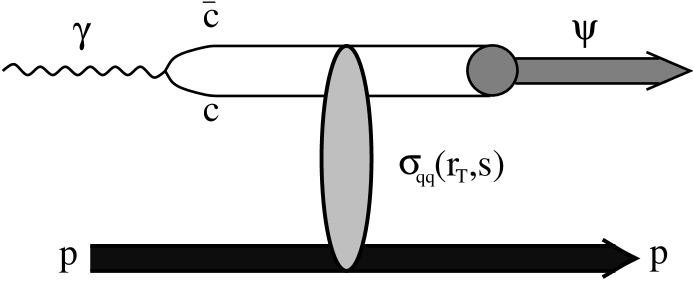
Figure 1: Schematic representation of the amplitude for the reaction $\gamma p\to\Psi p$ in the rest frame of the proton. The $c\bar{c}$ fluctuation of the photon with transverse separation $r_{T}$ and c.m. energy $\sqrt{s}$ interacts with the target proton via the dipole cross section ${\sigma_{q\bar{q}}}(r_{T},s)$ and produces a $\Psi$.

The corresponding expression for the forward amplitude reads

$${\cal M}_{\gamma p}(s,Q^{2})=\sum_{\mu,\bar{\mu}}\,\int\limits_{0}^{1}\!\!d\alpha\int d^{2}{\vec{r}_{T}}\,\Phi^{\!*(\mu,\bar{\mu})}_{\Psi}(\alpha,{\vec{r}_{T}})\,{\sigma_{q\bar{q}}}(r_{T},s)\,\Phi^{(\mu,\bar{\mu})}_{\gamma}(\alpha,{\vec{r}_{T}},Q^{2})\,.$$ (1)

Here the summation runs over spin indexes $\mu$, $\bar{\mu}$ of the $c$ and $\bar{c}$ quarks, $Q^{2}$ is the photon virtuality, $\Phi_{\gamma}(\alpha,r_{T},Q^{2})$ is the LC distribution function of the photon for a $c\bar{c}$ fluctuation of separation $r_{T}$ and relative fraction $\alpha$ of the photon LC momentum carried by $c$ or $\bar{c}$. Correspondingly, $\Phi_{\Psi}(\alpha,{\vec{r}_{T}})$ is the LC wave function of ${J\!/\!\psi}$ or $\psi^{\prime}$. The dipole cross section $\sigma_{q\bar{q}}(r_{T},s)$ mediates the transition.

This paper is organized as follows. First we review the expressions of the factorized LC approach to electroproduction of heavy quarkonia (more details one can find in HIKT ) and then compare with available experimental data for $J/\psi$ production. The calculations which are parameter free demonstrate good agreement with data.

After it we analyse exclusive electroproduction of charmonia off nuclei $\gamma A\to\Psi X$, where $X=A$ (coherent) or $X=A^{*}$ (incoherent, where $A^{*}$ is an exited state of the $A$-nucleon system). In these processes new phenomena are to be expected. (i) Color filtering, i.e. inelastic interactions of the $c\bar{c}$ pair on its way through the nucleus is expected to lead to a suppression of $\Psi$ production relative to $A\sigma_{\gamma p\to\Psi p}$. (ii) Production of a $c\bar{c}$ pair in a nucleus and its absorption are also determined by the values of the coherence length (lifetime of the $c\bar{c}$ fluctuation),

$$l_{c}=\frac{2\,\nu}{Q^{2}+M_{c\bar{c}}^{2}}\approx\frac{2\,\nu}{Q^{2}+M_{{J\!/\!\psi}}^{2}}\,,$$ (2)

where $\nu$ is the energy of the virtual photon in the rest frame of the nucleus. (iii) Since the dipole cross section ${\sigma_{q\bar{q}}}$ also depends on the gluon distribution in the target ($p$ of $A$), nuclear shadowing of the gluon distribution is expected to reduce ${\sigma_{q\bar{q}}}$ in a nuclear reaction relative to the one on the proton.

The predictions in this paper may be used for planning of future experiments for electron-nucleus collisions at high energies like in the eRHIC project. Another possibility to observe photoproduction off nuclei is heavy ion relativistic collisions (see, for example, review BHT ). In the last section we present our results for ${J\!/\!\psi}$ production in such processes.

2 Light-cone dipole approach

The LC variable describing longitudinal motion of the quarks is the fraction $\alpha=p_{c}^{+}/p_{\gamma}^{+}$ of the photon LC momentum $p_{\gamma}^{+}=E_{\gamma}+p_{\gamma}$ carried by the quark or antiquark. $\alpha$ is Lorentz-boost invariant. In the nonrelativistic approximation (assuming no relative motion of $c$ and $\bar{c}$) $\alpha=1/2$ (e.g. KZ ), otherwise one should integrate over $\alpha$ (see Eq. (1)).

2.1 Photon wave function

For transversely ($T$) and longitudinally ($L$) polarized photons the perturbative photon-quark distribution function in Eq. (1) reads KS ; BKS ,

$$\Phi_{T,L}^{(\mu,\bar{\mu})}(\alpha,{\vec{r}_{T}},Q^{2})=\frac{\sqrt{N_{c}\,\alpha_{em}}}{2\,\pi}\,Z_{c}\,\chi_{c}^{\mu\dagger}\,\widehat{O}_{T,L}\,\widetilde{\chi}_{\bar{c}}^{\bar{\mu}}\,K_{0}(\epsilon r_{T})\ ,$$ (3)

where $\widetilde{\chi}_{\bar{c}}=i\sigma_{y}\chi^{*}_{\bar{c}}$, $\chi$ and $\bar{\chi}$ are the spinors of the $c$-quark and antiquark respectively; $Z_{c}=2/3$. $K_{0}(\epsilon r_{T})$ is the modified Bessel function with $\epsilon^{2}=\alpha(1-\alpha)Q^{2}+m_{c}^{2}$. The operators $\widehat{O}_{T,L}$ have the form:

$$\widehat{O}_{T} = m_{c}\,\vec{\sigma}\cdot\vec{e}_{\gamma}+i(1-2\alpha)\,(\vec{\sigma}\cdot\vec{n})\,(\vec{e}_{\gamma}\cdot\vec{\nabla}_{r_{T}})+(\vec{n}\times\vec{e}_{\gamma})\cdot\vec{\nabla}_{r_{T}}\ ,$$ (4)

$$\widehat{O}_{L} = 2\,Q\,\alpha(1-\alpha)\,\vec{\sigma}\cdot\vec{n}\ ,$$ (5)

where $\vec{n}=\vec{p}/p$ is a unit vector parallel to the photon momentum and $\vec{e}$ is the polarization vector of the photon. Effects of the non-perturbative interaction within the $q\bar{q}$ fluctuation are negligible for the heavy charmed quarks.

2.2 Charmonium wave function

The charmonium wave function is well defined in its rest frame where one can rely on the Schrödinger equation. As soon as the rest frame wave function is known, one may be tempted to apply the Lorentz transformation to the $c\bar{c}$ pair as it would be a classical system and boost it to the infinite momentum frame. However, quantum effects are important and in the infinite momentum frame a series of different Fock states emerges from the Lorentz boost. Therefore the lowest $|c\bar{c}\rangle$ component in the infinite momentum frame does not represent the $|c\bar{c}\rangle$ in the rest frame. We rely on the widely used procedure Terent'ev for the generation of the LC wave functions of charmonia.

In the rest frame the spatial part of the $c\bar{c}$ pair wave function satisfying the Schrödinger equation

$$\left(-\,\frac{\Delta}{m_{c}}+V(r)\right)\,\Psi_{nlm}({\vec{r}\,})=E_{nl}\,\Psi_{nlm}({\vec{r}\,})$$ (6)

is represented in the form

$$\Psi({\vec{r}\,})=\Psi_{nl}(r)\cdot Y_{lm}(\theta,\varphi)\ ,$$ (7)

where ${\vec{r}\,}$ is 3-dimensional $c\bar{c}$ separation, $\Psi_{nl}(r)$ and $Y_{lm}(\theta,\varphi)$ are the radial and orbital parts of the wave function. The following four potentials $V(r)$ have been used

• “COR”: Cornell potential COR ,

  $$V(r)=-\frac{k}{r}+\frac{r}{a^{2}}$$ (8)

  with $k=0.52$, $a=2.34\,\mbox{GeV}^{-1}$ and $m_{c}=1.84\,\mbox{GeV}$.

• “BT”: Potential suggested by Buchmüller and Tye BT with $m_{c}=1.48\,\mbox{GeV}$. It has a similar structure as the Cornell potential: linear string potential at large separations and Coulomb shape at short distances with some refinements, however.

• “LOG”: Logarithmic potential LOG

  $$V(r)=-0.6635\,\mbox{GeV}+(0.733\,\mbox{GeV})\log(r\cdot 1\,\mbox{GeV})$$ (9)

  with $m_{c}=1.5\,\mbox{GeV}$.

• “POW”: Power-law potential POW

  $$V(r)=-8.064\,\mbox{GeV}+(6.898\,\mbox{GeV})(r\cdot 1\,\mbox{GeV})^{0.1}$$ (10)

  with $m_{c}=1.8\,\mbox{GeV}$.

The shapes of the four potentials differ from each other only at large $r$ ($\geq 1\,\mbox{fm}$) and very small $r$ ($\leq 0.05\,\mbox{fm}$) separations. Note, however, that COR and POW use $m_{c}\approx 1.8\,\mbox{GeV}$, while BT and LOG use $m_{c}\approx 1.5\,\mbox{GeV}$ for the mass of the charmed quark. This difference will have significant consequences.

For the ground state $1S$ all the potentials provide a very similar behavior for the radial part $\Psi_{nl}(r)$ at $r>0.3\,\mbox{fm}$, while for small $r$ the predictions differ by up to $30\%$. The peculiar property of the $2S$ state wave function is the node at $r\approx 0.4\,\mbox{fm}$ which causes strong cancellations in the matrix elements Eq. (1) and as a result, a suppression of photoproduction of $\psi^{\prime}$ relative to ${J\!/\!\psi}$ KZ ; Benhar .

The lowest Fock component $|c\bar{c}\rangle$ in the infinite momentum frame is not related by simple Lorentz boost to the wave function of charmonium in the rest frame. This makes the problem of building the LC wave function for the lowest $|c\bar{c}\rangle$ component difficult, no unambiguous solution is yet known. There are only recipes in the literature, a simple one widely used Terent'ev , is the following. One applies a Fourier transformation from coordinate to momentum space to the known spatial part of the non-relativistic wave function (7), $\Psi({\vec{r}\,})\Rightarrow\Psi({\vec{p}\,})$, which can be written as a function of the effective mass of the $c\bar{c}$, $M^{2}=4(p^{2}+m_{c}^{2})$, expressed in terms of LC variables

$$M^{2}(\alpha,p_{T})=\frac{p_{T}^{2}+m_{c}^{2}}{\alpha(1-\alpha)}\ .$$ (11)

In order to change integration variable $p_{L}$ to the LC variable $\alpha$ one relates them via $M$, namely $p_{L}=(\alpha-1/2)M(p_{T},\alpha)$. In this way the $c\bar{c}$ wave function acquires a kinematical factor

$$\Psi({\vec{p}\,})\Rightarrow\sqrt{2}\,\frac{(p^{2}+m_{c}^{2})^{3/4}}{(p_{T}^{2}+m_{c}^{2})^{1/2}}\cdot\Psi(\alpha,{\vec{p}_{T}})\equiv\Phi_{\psi}(\alpha,{\vec{p}_{T}})\ .$$ (12)

This procedure was used in Hoyer and the result is applied to calculation of the amplitudes (1). The result was discouraging, since the $\psi^{\prime}$ to ${J\!/\!\psi}$ ratio of the electroproduction cross sections are far too low in comparison with data. However, the oversimplified dipole cross section $\sigma_{q\bar{q}}(r_{T})\propto r_{T}^{2}$ was used, and what is even more essential, the important ingredient of Lorentz transformations, the Melosh spin rotation, was left out.

The 2-dimensional spinors $\chi_{c}$ and $\chi_{\bar{c}}$ describing $c$ and $\bar{c}$ respectively in the infinite momentum frame are known to be related via the Melosh rotation Terent'ev ; Melosh to the spinors $\bar{\chi}_{c}$ and $\bar{\chi}_{\bar{c}}$ in the rest frame: $\bf\overline{\chi}_{c}=\widehat{R}(\alpha,{\vec{p}_{T}})\,\chi_{c}$ and $\bf\overline{\chi}_{\bar{c}}=\widehat{R}(1-\alpha,-{\vec{p}_{T}})\,\chi_{\bar{c}}$, where the matrix $R(\alpha,{\vec{p}_{T}})$ has the form:

$$\widehat{R}(\alpha,{\vec{p}_{T}})=\frac{m_{c}+\alpha\,M-i\,[\vec{\sigma}\times\vec{n}]\,{\vec{p}_{T}}}{\sqrt{(m_{c}+\alpha\,M)^{2}+p_{T}^{2}}}\ .$$ (13)

Since the potentials we use contain no spin-orbit term, the $c\bar{c}$ pair is in $S$-wave. In this case spatial and spin dependences in the wave function factorize and we arrive at the following LC wave function of the $c\bar{c}$ in the infinite momentum frame

$$\Phi^{(\mu,\bar{\mu})}_{\psi}(\alpha,{\vec{p}_{T}})=U^{(\mu,\bar{\mu})}(\alpha,{\vec{p}_{T}})\cdot\Phi_{\psi}(\alpha,{\vec{p}_{T}})\ ,$$ (14)

where

$$U^{(\mu,\bar{\mu})}(\alpha,{\vec{p}_{T}})=\chi_{c}^{\mu\dagger}\,\widehat{R}^{\dagger}(\alpha,{\vec{p}_{T}})\,\vec{\sigma}\cdot\vec{e}_{\psi}\,\sigma_{y}\,\widehat{R}^{*}(1-\alpha,-{\vec{p}_{T}})\,\sigma_{y}^{-1}\,\widetilde{\chi}_{\bar{c}}^{\bar{\mu}}\,.$$ (15)

Now we can determine the LC wave function in the mixed longitudinal momentum - transverse coordinate representation:

$$\Phi^{(\mu,\bar{\mu})}_{\psi}(\alpha,{\vec{r}_{T}})=\frac{1}{2\,\pi}\int d^{2}{\vec{p}_{T}}\,e^{-i{\vec{p}_{T}}{\vec{r}_{T}}}\,\Phi^{(\mu,\bar{\mu})}_{\psi}(\alpha,{\vec{p}_{T}})\ .$$ (16)

2.3 Phenomenological dipole cross section

The color dipole cross section $\sigma_{q\bar{q}}(r_{T},s)$ is poorly known from first principles. It is expected to vanish $\propto r_{T}^{2}\,\ln r_{T}$ at small $r_{T}\!\!\to\!0$ due to color screening ZKL and to level off at large separations. We use a phenomenological form which interpolates between the two limiting cases of small and large separations. Few parameterizations are available in the literature, we choose two of them which are simple, but quite successful in describing data and denote them by the initials of the authors as “GBW” GBW and “KST” KST .

$$\mbox{``GBW'':}~{}~{}~{}~{}~{}~{}~{}~{}\sigma_{q\bar{q}}(r_{T},x) = 23.03\left[1-e^{-r_{T}^{2}/r_{0}^{2}(x)}\right]\,\mbox{mb}\ ,$$ (17)

$$r_{0}(x) = 0.4\left(\frac{x}{x_{0}}\right)^{\!\!0.144}\,\mbox{fm}\ ,$$

where $x_{0}=3.04\cdot 10^{-4}$. The proton structure function calculated with this parameterization fits well all available data at small $x$ and in wide range of $Q^{2}$ GBW . However, it obviously fails describing the hadronic total cross sections, since it never exceeds the value $23.03\,\mbox{mb}$. The $x$-dependence guarantees Bjorken scaling for DIS at high $Q^{2}$, however, Bjorken $x$ is not a well defined quantity in the soft limit. Instead we use the prescription of Ryskin , $x=(M^{2}_{\psi}+Q^{2})/s$, where $M_{\psi}$ is the charmonium mass.

This problem with limited dipole cross section as well as the difficulty with the definition of $x$ have been fixed in KST . The dipole cross section is treated as a function of the c.m. energy $\sqrt{s}$, rather than $x$, since $\sqrt{s}$ is more appropriate for hadronic processes. A similarly simple form for the dipole cross section is used

$$\mbox{``KST'':}~{}~{}~{}~{}~{}~{}~{}~{}~{}\sigma_{\bar{q}q}(r_{T},s) = \sigma_{0}(s)\left[1-e^{-r_{T}^{2}/r_{0}^{2}(s)}\right]\ .~{}~{}~{}~{}~{}~{}$$ (18)

The values and energy dependence of hadronic cross sections are reproduced with the following expressions

$$\sigma_{0}(s) = 23.6\left(\frac{s}{s_{0}}\right)^{\!\!0.08}\left(1+\frac{3}{8}\frac{r_{0}^{2}(s)}{\left<r^{2}_{ch}\right>}\right)\,\mbox{mb}\ ,$$ (19)

$$r_{0}(s) = 0.88\left(\frac{s}{s_{0}}\right)^{\!\!-0.14}\,\mbox{fm}\ .$$ (20)

The energy dependent radius $r_{0}(s)$ is fitted to data for the proton structure function $F^{p}_{2}(x,Q^{2})$, $s_{0}=1000\,\mbox{GeV}^{2}$ and the mean square of the pion charge radius $\left<r^{2}_{ch}\right>=0.44\,\mbox{fm}^{2}$. The improvement at large separations leads to a somewhat worse description of the proton structure function at large $Q^{2}$. Apparently, the cross section dependent on energy, rather than $x$, cannot provide Bjorken scaling. Indeed, parameterization (18) is successful only up to $Q^{2}\approx 10\,\mbox{GeV}^{2}$.

In fact, the cases we are interested in, charmonium production and interaction, are just in between the regions where either of these parameterization is successful. Therefore, we suppose that the difference between predictions using Eq. (17) and (18) is a measure of the theoretical uncertainty which fortunately turns out to be rather small.

3 Electroproduction off protons

Having Eq. (1) and the expressions from the previous section (LC wave functions and dipole cross section), we can calculate cross sections for the virtual photoproduction $\gamma p\to\Psi p$

$$\sigma_{\gamma p\to\Psi p}(s,Q^{2})=\frac{|\widetilde{\cal M}_{T}(s,Q^{2})|^{2}+\varepsilon\,|\widetilde{\cal M}_{L}(s,Q^{2})|^{2}}{16\,\pi\,B}\ ,$$ (21)

where $\varepsilon$ is the photon polarization (for H1 data $\langle\varepsilon\rangle=0.99$); $B$ is the slope parameter in reaction $\gamma^{*}p\to\psi p$. We use the experimental value H1-s $B=4.73\,GeV^{-2}$. $\widetilde{\cal M}_{T,L}$ includes also the correction for the real part of the amplitude:

$$\widetilde{\cal M}_{T,L}(s,Q^{2})={\cal M}_{T,L}(s,Q^{2})\,\left(1-i\,\frac{\pi}{2}\,\frac{\partial\,\ln{\cal M}_{T,L}(s,Q^{2})}{\partial\,\ln s}\right)\ ,$$ (22)

where we apply the well known derivative analyticity relation between the real and imaginary parts of the forward elastic amplitude Bronzan . The correction from the real part is not small since the cross section of charmonium electroproduction is a rather steep function of energy.

Figure 2: Integrated cross section for elastic photoproduction with real photons ($Q^{2}=0$) calculated with GBW and KST dipole cross sections and for four potentials to generate ${J\!/\!\psi}$ wave functions. Experimental data points from the H1 H1-s , E401 E401-s , E516 E516-s and ZEUS ZEUS-s experiments.

Figure 3: The ratio of $\psi^{\prime}$ to $J/\psi$ virtual photoproduction cross sections as a function of the photon virtuality $Q^{2}$ at energy $\sqrt{s}=90\,\mbox{GeV}$ for four potentials and with GBW and KST parameterizations for the dipole cross section. Experimental data points from the H1 experiment H1-RQ .

We present here only results for energy dependence of the ${J\!/\!\psi}$ integrated cross section (Fig. 2) and for $Q^{2}$ dependence of the ratio $\psi^{\prime}$ to ${J\!/\!\psi}$ photoproduction (Fig. 3). More results are presented in HIKT . All calculations are performed with GBW and KST parameterizations for the dipole cross section and for wave functions of the ${J\!/\!\psi}$ calculated from BT, LOG, COR and POW potentials. One can see that there are no major differences for the results using the GBW and KST parameterizations. The BT and LOG potentials describe the data very well, while the potentials COR and POW underestimate them by a factor of two. The different behavior has been traced to the following origin: BT and LOG use $m_{c}\approx 1.5\,\mbox{GeV}$, but COR and POW $m_{c}\approx 1.8\,\mbox{GeV}$. While the bound state wave functions of ${J\!/\!\psi}$ are little affected by this difference, the photon wave function Eq. (3) depends sensitively on $m_{c}$.

It turns out that the effects of spin rotation have a gross impact on the ratio $R=\sigma(\psi^{\prime})/\sigma({J\!/\!\psi})$. This effects add 30-40% to the ${J\!/\!\psi}$ electroproduction cross section. But they have a much more dramatic impact on $\psi^{\prime}$ increasing the electroproduction cross section by a factor 2-3. This spin effects explain the large values of the ratio $R$ observed experimentally. Our results for $R$ are about twice as large as evaluated in Suzuki and even more than in Hoyer .

4 Electroproduction off nuclei

Exclusive charmonium production off nuclei, $\gamma A\to\Psi X$ is called coherent, when the nucleus remains intact, i.e. $X=A$, or incoherent, when $X$ is an excited nuclear state which contains nucleons and nuclear fragments but no other hadrons. The cross sections depend on the polarization $\varepsilon$ of the virtual photon (in all figures below we will imply $\varepsilon=1$),

$$\sigma_{\gamma A}(s,Q^{2})=\sigma_{T}(s,Q^{2})+\varepsilon\,\sigma_{L}(s,Q^{2})~{},$$ (23)

where the indexes $T,L$ correspond to transversely or longitudinally polarized photons, respectively. At high energies the coherence length Eq. (2) may substantially exceed the nuclear radius ($l_{c}\gg R_{A}$). In this case the transverse size of the $c\bar{c}$ wave packet is “frozen” by Lorentz time dilation, i.e. it does not fluctuate during propagation through the nucleus, and the expressions for the incoherent ($inc$) and coherent ($coh$) cross sections are simple KZ :

$$\sigma_{T,L}^{coh}(s,Q^{2}) = \int d^{2}b\left|\widetilde{\cal M}_{T,L}^{coh}(s,Q^{2},b)\right|^{2}\,,$$ (24)

$$\sigma_{T,L}^{inc}(s,Q^{2}) = \int d^{2}b\left|\widetilde{\cal M}_{T,L}^{inc}(s,Q^{2},b)\right|^{2}\,\frac{T_{A}(b)}{16\pi B(s)}\,,$$ (25)

where $T_{A}(b)=\int_{-\infty}^{\infty}dz\,\rho_{A}(b,z)$ is the nuclear thickness function given by the integral of the nuclear density along the trajectory at a given impact parameter $b$ and expressions for $\widetilde{\cal M}(s,Q^{2},b)$ are given by Eqs. (22) and (1) with replacement

$${\sigma_{q\bar{q}}}(r_{T},s)\Rightarrow\left\{\begin{array}[]{rl}1-\exp\left[-{\sigma_{q\bar{q}}}(r_{T},s)\,T_{A}(b)/2\right],&coh.\\[5.69054pt] {\sigma_{q\bar{q}}}(r_{T},s)\exp\left[-{\sigma_{q\bar{q}}}(r_{T},s)\,T_{A}(b)/2\right],&inc.\end{array}\right.$$ (26)

But for charmonium production off nuclei the “frozen” approximation is not enough and additional phenomena should be taken into account: effects of finite coherence length and gluon shadowing.

4.1 Finite coherence length

The “frozen” approximation (26) is valid only for $l_{c}\gg R_{A}$ and can be used only at $\sqrt{s}>20\div 30\,\,\mbox{GeV}$. The low-energy part should be corrected for the effects related to the finiteness of $l_{c}$. A strictly quantum-mechanical treatment of a fluctuating $q\bar{q}$ pair propagating through an absorptive medium based on the LC Green function approach has been suggested recently in KNST . However, an analytical solution for the LC Green function is known only for the simplest form of the dipole cross section ${\sigma_{q\bar{q}}}(r_{T})\propto r_{T}^{2}$. With a realistic form of ${\sigma_{q\bar{q}}}(r_{T})$ it is possible only to solve this problem numerically, what is still a challenge. Here we use the approximation suggested in HKZ to evaluate the corrections arising from the finiteness of $l_{c}$ by multiplying the cross sections for coherent and incoherent production evaluated for $l_{c}\to\infty$ by a kind of formfactor $F^{coh}$ and $F^{inc}$ respectively:

$$\sigma_{\gamma A}(s,Q^{2})\Rightarrow\sigma_{\gamma A}(s,Q^{2})\cdot F\left(s,l_{c}(s,Q^{2})\right)\,,$$ (27)

where

$$F^{coh}(s,l_{c}) = \int\!d^{2}b\left|\,\int\limits_{-\infty}^{\infty}\!dz\,\rho_{A}(b,z)\,F_{1}(s,b,z)\,e^{iz/l_{c}}\right|^{2}/\,(...)|_{l_{c}=\infty}\,,$$ (28)

$$F^{inc}(s,l_{c}) = \int\!d^{2}b\,\int\limits_{-\infty}^{\infty}\!dz\,\rho_{A}(b,z)\,\left|F_{1}(s,b,z)-F_{2}(s,b,z,l_{c})\right|^{2}/\,(...)|_{l_{c}=\infty}\,,$$ (29)

$$F_{1}(s,b,z) = \,\exp\left(-\frac{1}{2}\,\sigma_{\Psi N}(s)\!\int\limits_{z}^{\infty}\!dz^{\prime}\,\rho_{A}(b,z^{\prime})\right)\,,$$ (30)

$$F_{2}(s,b,z,l_{c}) = \frac{1}{2}\,\sigma_{\Psi N}(s)\!\int\limits_{-\infty}^{z}\!dz^{\prime}\,\rho_{A}(b,z^{\prime})\,F_{1}(b,z^{\prime})\,e^{-i(z-z^{\prime})/l_{c}}\,.$$ (31)

For the charmonium nucleon total cross section $\sigma_{\Psi N}(s)$ we use our previous results HIKT .

4.2 Gluon shadowing

The gluon density in nuclei at small Bjorken $x$ is expected to be suppressed compared to a free nucleon due to interferences. This phenomenon, called gluon shadowing, renormalizes the dipole cross section,

$${\sigma_{q\bar{q}}}(r_{T},x)\Rightarrow{\sigma_{q\bar{q}}}(r_{T},x)\,R_{G}(x,Q^{2},b)\,.$$ (32)

where the factor $R_{G}(x,Q^{2},b)$ is the ratio of the gluon density at $x$ and $Q^{2}$ in a nucleon of a nucleus to the gluon density in a free nucleon. No data are available so far which could provide information about gluon shadowing. Currently it can be evaluated only theoretically. To calculate function $R_{G}$ we use the approach developed in KST and applied for charmonia production in HIKT-A .

4.3 Numerical results

Combining the results above (i.e. including finite coherence length and gluon shadowing) we obtain the results for charmonia (${J\!/\!\psi}$ and $\psi^{\prime}$) electroproduction off nuclei. As it is common practice we express nuclear cross sections in the form of the ratio

$$R_{\Psi}(s,Q^{2})=\frac{\sigma_{\gamma A}(s,Q^{2})}{A\,\sigma_{\gamma p}(s,Q^{2})}~{},$$ (33)

where the numerator stands for the expression Eq. (23) (with Eq. (24) for coherent and Eq. (25) for incoherent scattering) and the denominator is given by Eq. (21). We present here only $s$ dependences (plots for $Q^{2}$ dependences and momentum transfer $\vec{k}_{T}$ distributions are given in HIKT-A ) for coherent (Fig. 4) and incoherent (Fig. 5) production of charmonia with the GBW GBW parameterization for the dipole cross section. KST KST parameterization gives quite close results (they differ at most 10% at high energies). It is not a surprise that the ratios for coherent production exceed one: in the absence of $c\bar{c}$ attenuation the forward coherent production would be proportional to $A^{2}$, while integrated over momentum transfer it behaves as $A^{4/3}$. It is a result of our definition Eq. (33) that $R^{coh}_{\Psi}$ exceeds one.

   

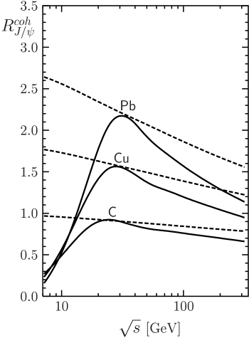
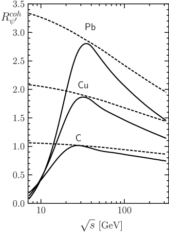
Figure 4: Ratios $R^{coh}_{{J\!/\!\psi}}$ and $R^{coh}_{\psi^{\prime}}$ for coherent production on carbon, copper and lead as a function of $\sqrt{s}$ and at $Q^{2}=0$ calculated with GBW parameterization of ${\sigma_{q\bar{q}}}$. Solid curves display the modifications due to the finite coherence length $l_{c}$ and gluon shadowing corrections while the dashed lines are without (“frozen” approximation).

   

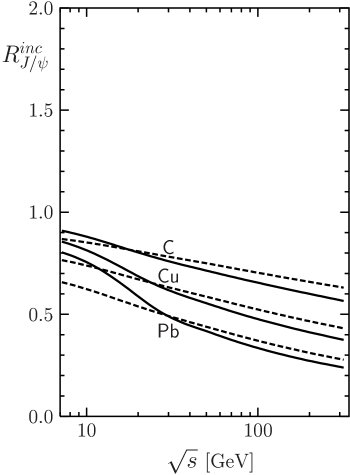
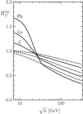
Figure 5: Ratios $R^{inc}_{\Psi}$ for ${J\!/\!\psi}$ and $\psi^{\prime}$ incoherent production on nuclei as function of $\sqrt{s}$ and at $Q^{2}=0$. The meaning of the different lines is the same as in Fig. 4.

We see that in comparison with the “frozen” approximation, $l_{c}$ corrections noticeable change ratios at low energies (especially for $\psi^{\prime}$). For coherent production in the limit of low energies $l_{c}\to 0$ the strongly oscillating exponential phase factor in (28) makes the integral very small and thus $F^{coh}\approx 0$. Then the cross section rises with $l_{c}$ unless it saturates at $l_{c}\gg R_{A}$ when the phase factor becomes constant. Apparently, this transition region is shifted to higher energies for larger nuclear radius. For incoherent production the observed nontrivial energy dependence is easy to interpret. At low energies $l_{c}\ll R_{A}$ and the photon propagates without any attenuation inside the nucleus where it develops for a short time $t_{c}$ a $c\bar{c}$ fluctuation which momentarily interacts to get on mass shell. The produced $c\bar{c}$ pair attenuates along the path whose length is a half of the nuclear thickness on the average. On the other hand, at high energies when $l_{c}\gg R_{A}$ the $c\bar{c}$ fluctuation develops long before its interaction with the nucleus. As a result, it propagates through the whole nucleus and the mean path is twice as long as at low energies. This is why the nuclear transparency drops when going from the regimes of short to long $l_{c}$.

At high energies gluon shadowing becomes important. We see that the onset of gluon shadowing happens at a c.m. energy of few tens of GeV. Remarkably, the onset of shadowing is delayed with rising nuclear radius. Nuclear suppression of ${J\!/\!\psi}$ production becomes stronger with energy. This is an obvious consequence of the energy dependence of ${\sigma_{q\bar{q}}}(r_{T},s)$, which rises with energy. For $\psi^{\prime}$ the suppression is rather similar as for ${J\!/\!\psi}$. In particular we do not see any considerable nuclear enhancement of $\psi^{\prime}$ which has been found earlier KZ ; KNNZ , where the oversimplified form of the dipole cross section, ${\sigma_{q\bar{q}}}(r_{T})\propto r_{T}^{2}$ and the oscillator form of the wave function had been used.

5 Heavy ion peripheral collisions

The large charge $Z$ of heavy nuclei gives rise to strong electromagnetic fields: the photon field of one nucleus can produce a photo-nuclear interaction in the other. The cross section of the charmonia photoproduction by the induced photons reads

$$k\frac{d\sigma}{dk}=\int\!\!d^{2}b\int\!\!d^{2}b^{\prime}\,n(k,\vec{b}^{\prime}-\vec{b})\,\sigma_{A}(b,s)\,,$$ (34)

where $k$ is the photon momentum. Photon flux induced by projectile nucleus with Lorenz factor $\gamma$ is

$$n(k,\vec{b})=\frac{{\alpha_{\mbox{\tiny em}}}Z^{2}k^{2}}{\pi^{2}{\gamma}^{2}}K_{1}^{2}\left(\frac{bk}{\gamma}\right)\,.$$ (35)

Cross sections $\sigma_{A}(b,s)$ for coherent and incoherent production are

$$\sigma_{A}^{coh}(s,b) = \left|\widetilde{\cal M}_{A}^{coh}(s,b)\right|^{2}\,,$$ (36)

$$\sigma_{A}^{inc}(s,b) = \left|\widetilde{\cal M}_{A}^{inc}(s,b)\right|^{2}\,\frac{T(b)}{16\pi B(s)}\,,$$ (37)

where expressions $\widetilde{\cal M}(s,b)$ correspond to $\widetilde{\cal M}$ in Eqs. (24, 25) at $Q^{2}=0$. Our predictions for coherent ${J\!/\!\psi}$ production at RHIC and LHC energies are presented on Fig. 6.

   

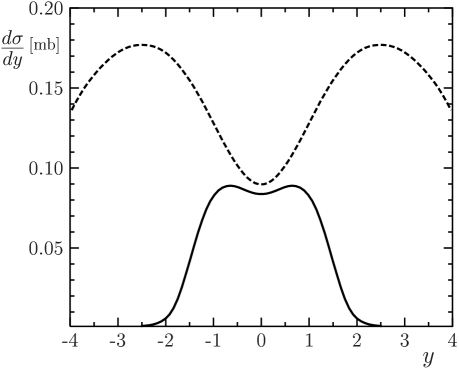
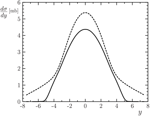
Figure 6: Rapidity distribution for coherent ${J\!/\!\psi}$ production in heavy ion peripheral gold-gold collisions at RHIC (left) and lead-lead collisions at LHC (right) calculated with the GBW parameterization of ${\sigma_{q\bar{q}}}$. Solid curves display the modifications due to gluon shadowing and finite coherence length $l_{c}$ while the dashed lines are without (“frozen” approximation).

We see that $l_{c}$ corrections modify the distribution at the edges (positive and negative $y$) while suppression around $y=0$ is provided mostly by gluon shadowing (especially for LHC, where energies should be much higher).

6 Conclusion

In this paper we use the LC dipole approach for description of charmonium electroproduction off protons and nuclei. We have no free parameters and our calculations are in good agreement with existing experimental data. Our predictions can be tested in future experiments at high energies with electron-nuclear colliders (eRHIC) and in peripheral heavy ion collisions (RHIC and LHC).

Acknowledgment: The authors gratefully acknowledge the partial support by a grant from the Gesellschaft für Schwerionenforschung Darmstadt (grant no. GSI-OR-SCH) and by the Federal Ministry BMBF (grant no. 06 HD 954).

References

- (1) Kopeliovich, B.Z., and Zakharov, B.G., Phys. Rev. D 44, 3466 (1991).
- (2) Huefner, J., et al., Phys. Rev. D 62, 094022 (2000); hep-ph/0007111.
- (3) Huefner, J., et al., Phys. Rev. C 66, 024903 (2002); hep-ph/0202216.
- (4) Baur, G., Hencken, K., and Trautmann, D., Prog. Part. Nucl. Phys. 42, 357 (1999); nucl-th/9810078.
- (5) Kogut, J.B., and Soper, D.E., Phys. Rev. D1 2901 (1970).
- (6) Bjorken, J.M., Kogut, J.B., and Soper, D.E., Phys. Rev. D3 1382 (1971).
- (7) Zamolodchikov, A.B., Kopeliovich, B.Z., and Lapidus, L.I., JETP Lett. 33 595 (1981).
- (8) Golec-Biernat, K., and Wüsthoff, M., Phys. Rev. D53 014017 (1999); hep-ph/9903358.
- (9) Kopeliovich, B.Z., Schäfer, A., and Tarasov, A.V., Phys. Rev. D62 054022 (2000); hep-ph/9908245.
- (10) Ryskin, M.G., Roberts, R.G., Martin, A.D., and Levin, E.M., Z. Phys. C76 231 (1997).
- (11) Terent’ev, M.V., Sov. J. Nucl. Phys. 24 106 (1976).
- (12) Eichten, E., et al., Phys. Rev. D 17 3090 (1978); Phys. Rev. D 21 203 (1980).
- (13) Buchmüller, W., and Tye, S.-H.H., Phys. Rev. D 24 132 (1981).
- (14) Quigg, C., and Rosner, J.L., Phys. Lett. B 71 153 (1977).
- (15) Martin, A., Phys. Lett. B 93 338 (1980).
- (16) Benhar, O., et al., Phys. Rev. Lett. 69 1156 (1992).
- (17) Hoyer, P., and Peigné, S., Phys. Rev. D 61 031501 (2000).
- (18) Melosh, H.J., Phys. Rev. D 9 1095 (1974); Jaus, W., Phys. Rev. D 41 3394 (1990).
- (19) Bronzan, J.B., Kane, G.L., and Sukhatme, U.P., Phys. Lett. B 49 272 (1974).
- (20) H1 Collaboration, Adloff, C., et al., Phys. Lett. B 483 23-35 (2000); hep-ex/0003020.
- (21) E401 Collaboration, Binkley, M., et al., Phys. Rev. Lett. 48 73 (1982).
- (22) E516 Collaboration, Denby, B.H., et al., Phys. Rev. Lett. 52 795 (1984).
- (23) ZEUS Collaboration, Breitweg, J., et al., Z. Phys. C 75 215 (1997).
- (24) H1 Collaboration, Adloff, C., et al., Eur. Phys. J. C 10 373 (1999); hep-ex/9903008.
- (25) Suzuki, K., et al. Phys. Rev. D 62 031501 (2000); hep-ph/0005250.
- (26) Kopeliovich, B.Z., et al., Phys. Rev. C 65, 035201 (2002); hep-ph/0107227.
- (27) Hüfner, J., Kopeliovich, B.Z., and Zamolodchikov, Al.B., Z. Phys. A 357, 113 (1997).
- (28) Kopeliovich, B.Z., et al., Phys. Lett. B 324, 469 (1994).