Abstract

We have calculated the fermion contributions to the shift of the position of the poles of the massive gauge boson propagators at two–loop order in the Standard Model. Together with the bosonic contributions calculated previously the full two–loop corrections are available. This allows us to investigate the full correction in the relationship between $\overline{\rm MS}$ and pole masses of the vector bosons $Z$ and $W$. Two–loop renormalization and the corresponding renormalization group equations are discussed. Analytical results for the master–integrals appearing in the massless fermion contributions are given. A new approach of summing multiple binomial sums has been developed.

1 Introduction

In our previous paper [1], referred to as I in the following, we presented the two–loop calculation of the bosonic contributions to the $W$– and $Z$–self–energies on the mass shell and discussed the main properties and possible applications. In the present paper II we extend this calculation to a full Standard Model (SM) calculation by including the missing fermion–loop and mixed contributions. Throughout the paper, we shall adopt the terminology calling “bosonic corrections” the one’s represented by diagrams without any fermions and “fermionic corrections” the remaining one’s given by diagrams exhibiting at least one fermion loop.

In I, in particular, we have shown by an explicit calculation that up to two-loop order the purely bosonic corrections to the position of the pole of the gauge-boson propagators are real for arbitrary values of the Higgs-boson mass. In contrast, since the $W$– and $Z$–bosons decay, at leading order, into light fermion pairs, the light (massless) fermion corrections give rise to a non–zero imaginary part at the one loop level already. The problem of gauge (in)dependence of the complex pole has been extensively discussed in literature [2]. Only recently, two important results have been proven to all orders in perturbation theory: i) the position of the complex pole is a gauge independent quantity [3]; ii) the branching ratios and partial widths associated with the pole residues are gauge independent [4]. Moreover, it has been shown that the pole mass of the W-boson is an infrared finite quantity with respect to massless photonic corrections. An alternative proof of the infrared finiteness of the two-loop bosonic contributions to the pole of the gauge bosons was presented in I by explicite calculation. It is based on the fact that within dimensional regularization [5], in $d=4-2\varepsilon$ space-time dimensions, the singular $1/\varepsilon$ terms, which regularize both ultraviolet (UV) and infrared (IR) singularities, are absent after UV renormalization of the position of the pole in the propagators.

In the present paper, besides from completing our previous calculation by including the missing fermion contributions, we will discuss in some detail general features and technical problems which are specifically related to these contributions.

The paper is organized as follows. In Section 2 we briefly reconsider the definition of the pole-mass of the massive gauge-bosons within the SM and remind the reader of some notation given in I. The required analytical results for the massless fermion two-loop master-integrals are presented in Section 3. In Section 4 we discuss the UV renormalization of the pole mass and the interrelation between our results and the one’s familiar from the standard renormalization group approach. In particular, we performed several cross-checks of the singular $1/\varepsilon^{2}$- and $1/\varepsilon$-terms. General aspects as well as numerical results for the finite parts are discussed in Section 5. Some technical details and a number of our analytical results will be presented in Appendices. In Appendix A we present a set of non–standard binomial sums which are needed for the $\varepsilon$–expansion of some of the hypergeometric functions entering the master–integrals. The one–loop fermion contribution to the pole masses of the gauge–bosons are reproduced in Appendix B. The reducible two–loop corrections obtained by mass renormalization of the one–loop fermion contributions may be found in Appendix C. In Appendix D the bare two–loop on–shell self–energy contribution of the massless fermions are given in exact analytical form. The corresponding contributions involving the top quark are presented in terms of the first few coefficients of the expansion in $\sin^{2}\theta_{W}$ and specific mass ratios in Appendix E.

2 Pole mass: definition and calculation

The position of the pole $s_{P}$ of the propagator of a massive gauge-boson in a quantum field theory is a solution for $p^{2}$ at which the inverse of the connected full propagator equals zero, i.e.,

$$s_{P}-m^{2}-\Pi(s_{P},m^{2},\cdots)=0,$$ (2.1)

where $\Pi(p^{2},\cdots)$ is the transversal part of the one-particle irreducible self-energy. The latter depends on all SM parameters but, in order to the keep notation simple, we have indicated explicitly only the dependence on the external momentum $p$ and in some cases also $m$, where $m$ is the mass of the particle under consideration. This can be either the bare mass or the renormalized mass defined in some particular renormalization scheme.

Generally, the pole $s_{P}$ is located in the complex plane of $p^{2}$ and has a real and an imaginary part. By writing

$$s_{P}\equiv M^{2}-{\rm i}M\Gamma\;,$$ (2.2)

the real part defines $M$ which we call the pole mass while the imaginary part is related to the width $\Gamma$ of the particle. This is the natural generalization of the physical mass of a stable particle, which is defined by the mass of its asymptotic scattering state [6, 7].

For the remainder of the paper we will adopt the following notation: capital $M$ always denotes the pole mass; lower case $m$ stands for the renormalized mass in the $\overline{\rm MS}$ scheme, while $m_{0}$ denotes the bare mass. In addition we use $e$, $g$ and $g_{s}$ to denote the $U(1)_{\rm em}$, $SU(2)_{\rm L}$ and $SU(3)_{\rm c}$ couplings of the SM in the $\overline{\rm MS}$ scheme.

In perturbation theory (2.1) is to be solved order by order. To two loops we have the solution

$$s_{P} = m^{2}+\Pi^{(1)}(m^{2},m^{2},\cdots)+\Pi^{(2)}(m^{2},m^{2},\cdots)+\Pi^{(1)}(m^{2},m^{2},\cdots)\Pi^{(1)}{}^{\prime}(m^{2},m^{2},\cdots),$$ (2.3)

which yields the pole mass $M^{2}$ and the width $\Gamma$ at this order. $\Pi^{(L)}$ is the bare ($m=m_{0}$) or $\overline{\rm MS}$ -renormalized ($m$ the $\overline{\rm MS}$ -mass) $L$-loop contribution to $\Pi$, and the prime denotes the derivative with respect to $p^{2}$.

In this paper we show by explicit calculation at the two-loop level that the fermion contribution (including mixed terms) to the propagator pole $s_{P}$ of a gauge boson is a gauge invariant and infrared stable quantity. For more details concerning the tensor decomposition of propagators and abbreviations adopted we refer to Sec. 2 of I.

In order to find the relationship between the poles of the gauge boson-propagators and the $\overline{\rm MS}$ masses $m_{Z}^{2},\,m_{W}^{2}$ we have to compute the one- and two-loop self-energies for the $Z$- and $W$-bosons at $p^{2}=m_{Z}^{2}$ and $p^{2}=m_{W}^{2}$, respectively.

For the calculation of the two-loop fermion contributions we again use the strategy described in our previous paper I. Let us present here some basic features. In order to be able to work with manifestly gauge independent parameter renormalization constants we have to include the Higgs tadpole diagrams. To keep control of gauge invariance we work in the $R_{\xi}$ gauge with three different gauge parameters $\xi_{W},\,\xi_{Z}$ and $\xi_{\gamma}$. However, in order to avoid additional mass parameters like $\sqrt{\xi_{W}}m_{W}$ and $\sqrt{\xi_{Z}}m_{Z}$ (ghost masses), we expand the original propagators in an asymptotic series at $\xi_{i}=1$. For the purpose of checking the gauge invariance of our results it turned out to be sufficient to keep the first two terms of the expansion. As an additional cross–check we actually kept one more term.

For calculating diagrams with massless fermion loops we utilize Tarasov’s recurrence relations [11] (a detailed discussion we postpone to Sec. 3). For diagrams with top-quark and/or Higgs-boson propagators we apply asymptotic expansions with respect to the heavy masses. In these cases we firstly expand the propagator in the weak mixing parameter $\sin^{2}\theta_{W}=1-m_{W}^{2}/m_{Z}^{2}\approx 0.25$ and get rid in this way of $m_{W}$ (or $m_{Z}$). All diagrams with top-quarks and/or Higgs-bosons are divided into several prototypes which are presented in Fig. 1. The large mass expansion has been performed with the help of the packages TLAMM [12] or by the program described in [13]. In the heavy top limit, the leading and next–to–leading contributions to the gauge boson self–energies have been calculated in [14, 15] and  [16], respectively.

As usual, in order to preserve gauge invariance of the regularized theory, we utilize dimensional regularization [5] for our calculation. In order to avoid spurious anomalies we adopt an anti-commuting $\gamma_{5}$ in dimensional regularization [5, 17] and impose vector current conservation by hand in triangle fermion loops which contribute to the two–loop two–point functions [18]. The axial vector current anomalies [19] cancel for each fermion family by the lepton–quark duality [20]. In contrast to calculations which involve vertex- and/or box-type diagrams [21], in our calculation of self-energies we do not encounter problems with violation of Ward identities (see also [22]).

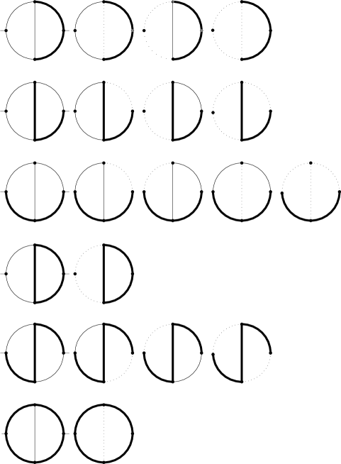
Figure 1: The prototype diagrams and their subgraphs contributing to the large mass expansion for two-loop diagrams with heavy propagators. Thick and thin lines correspond to heavy- and light-mass (massless) particle propagators, respectively. Dotted lines indicate the lines omitted in the subgraph.

3 Master integrals for the massless fermion contributions

This part is devoted to the calculation of the two-loop massless fermion corrections to the pole masses of the gauge bosons. For this class of corrections it is possible to work out the exact analytical results without expansion.

In contrast to the previous calculations performed in [22], where results are expressed in terms of the non–minimal set of scalar two–loop integrals, we use here Tarasov’s recurrence relations [11] which allow us to reduce the number of integrals to a minimal set of master–integrals in our results. The analytical results for these diagrams are presented in [23]. Here we present an independent analytical calculation of the relevant master integrals shown in Fig. 2. Besides the known one’s, we consider here two new master-integrals, shown in Fig. 3, which contribute to the two-loop on-shell top-quark propagator in the limit of massless gauge-bosons. They may also be considered as the “naive” parts of the asymptotic expansion of the original diagrams with massive $W$- and $Z$-bosons in the limit, when the external momentum approaches the heavy mass-shell [24].

Figure 2: Diagrams corresponding to the master–integrals with massless fermion-loops contributing to the two-loop gauge-boson propagators. Bold, thin and dashed lines correspond to off-shell massive, on-shell massive and to massless propagators, respectively.

Figure 3: Diagrams contributing to the two-loop on-shell top-quark propagator in the limit of massless gauge-bosons. Bold, thin and dashed lines correspond to off-shell massive, on-shell massive and to massless propagators, respectively.

For the analytical calculation of these integrals up to the finite parts in $\varepsilon$ we use the method developed in [25] (see also [26]). This approach is based on the possibility to retrieve the analytical results in terms of sums, as predicted by the differential equation method [27], from several of the first coefficients of the small momentum expansion [28]. Whenever it is possible, we present the exact analytical results in terms of hypergeometric functions. Thereby, we apply Mellin–Barnes techniques developed in [29, 30].

Let us introduce now the following notation for the finite sums which show up in the master integrals:

$$S_{a}(n)=\sum_{j=1}^{n}\frac{1}{j^{a}},~{}~{}~{}~{}~{}V_{a}(n)=\sum_{j=1}^{n}\frac{1}{\left(2j\atop j\right)}\frac{1}{j^{a}},~{}~{}~{}~{}~{}W_{a}(n)=\sum_{j=1}^{n}\left(2j\atop j\right)\frac{1}{j^{a}}\;.$$

Throughout the rest of this paper, the symbol $S_{a}$ will always stand for $S_{a}(n-1)$ and $\bar{S}_{a}$ will stand for $S_{a}(2n-1)$. The same notation applies for all the other type of sums, e.g., $V_{a}=V_{a}(n-1)$. We denote all master integrals as $T_{AB\cdots}$, where the first letter $T=F,V,J$ indicates the topology in accordance with notation introduced in [11]; indices $A,B,\cdots=0,1,2$ characterize the relation of the corresponding internal mass to the external momentum: $0$ indicates a massless line, $1$ corresponds to “internal mass equal to external momentum” and $2$ means that mass and momentum are different (see Fig. 2 for details). In our normalization each loop is divided by $(\pi)^{2-\varepsilon}\Gamma(1+\varepsilon).$

• $\bf F_{00002}$

For this integral we use the representation given in [25]

$$p^{2}\cdot F_{00002} = 2\zeta_{2}\ln(1+z)+2\ln(-z){\rm Li}_{2}(-z)+\ln^{2}(-z)\ln(1+z)+4\ln(1+z){\rm Li}_{2}(z)$$ (3.4)

$$-2{\rm Li}_{3}(-z)-2{\rm Li}_{3}(z)+2S_{1,2}(z^{2})-4S_{1,2}(z)-4S_{1,2}(-z)\,,$$

where $z=\frac{p^{2}}{M^{2}}$ and $S_{n,p}$ are Nielsen polylogarithms [31, 32]. For the on–shell gauge-boson propagators two points in the variable $z$ are interesting: (i) $z=\cos^{2}\theta_{W}[p^{2}=m_{W}^{2}]$; (ii)$z=1/\cos^{2}\theta_{W}[p^{2}=m_{Z}^{2}]$.

• $\bf F_{20200}$

For this integral the following representation is valid

$$p^{2}\cdot F_{20200} = {\mbox{Li}}_{3}\left(z\right)-6\zeta_{3}-\zeta_{2}\ln y-\frac{1}{6}\ln^{3}y-4\ln y\,{\mbox{Li}}_{2}\left(y\right)$$ (3.5)

$$+4{\mbox{Li}}_{3}\left(y\right)-3{\mbox{Li}}_{3}\left(-y\right)+\frac{1}{3}{\mbox{Li}}_{3}\left(-y^{3}\right)\;,$$

where we have introduced the new “conformal” variable

$$y=\frac{1-\sqrt{\frac{z}{z-4}}}{1+\sqrt{\frac{z}{z-4}}},~{}~{}~{}~{}z=-\frac{(1-y)^{2}}{y}\equiv\frac{p^{2}}{M^{2}}\;.$$ (3.6)

Here we are interested in the case $z=1/\cos^{2}\theta_{W}$ only.

• $\bf V_{2002}$

The off-shell integral $V_{X00Y}$ with two different masses and unit powers of propagators was considered in [33]. The result, Eq. (46) of [33] was presented as a sum of $F_{2}$ and $F_{4}$ hypergeometric functions of two variables. It turns out, however, that the extraction of the finite part from this result is difficult. The analytical result up to finite parts for this diagram (see Fig. 2) is given by

$$(M^{2})^{2\varepsilon}\,V_{2002}=-\frac{1}{2\varepsilon^{2}}-\frac{1}{2\varepsilon}-\frac{1}{2}-\zeta_{2}+\sum\limits_{n=1}^{\infty}z^{n}\Biggl{\{}\frac{1}{\varepsilon}\left[-\frac{1}{n}\frac{1}{{2n\choose n}}+4\frac{1}{n+1}\frac{1}{{2n+2\choose n+1}}\right]$$

$$-\frac{1}{n}-\frac{1}{2}\frac{1}{n^{2}}-\frac{1}{n}\frac{1}{{2n\choose n}}\Biggl{[}\frac{3}{2}W_{1}+S_{1}+4\Biggr{]}+\frac{1}{n+1}+\frac{1}{n+1}\frac{1}{{2n+2\choose n+1}}\Biggl{[}6W_{1}(n)+4S_{1}(n)+16\Biggr{]}\Biggr{\}},$$

(3.7)

where $z=p^{2}/M^{2}$ with $M$ an internal mass. This result can be written also as

$$\left(\frac{p^{2}}{z}\right)^{2\varepsilon}\,V_{2002}=-\frac{1}{2\varepsilon^{2}}-\frac{1}{\varepsilon}\Biggl{[}\frac{5}{2}+\frac{1+y}{1-y}\ln y\Biggr{]}-\frac{19}{2}-\zeta_{2}-\frac{1}{2}{\rm Li}_{2}(z)-\frac{1-z}{z}\ln(1-z)$$

$$+\frac{1+y}{1-y}\Biggl{[}\frac{7}{2}{\rm Li}_{2}(-y)-\frac{1}{2}{\rm Li}_{2}(-y^{3})-\frac{5}{4}\ln^{2}y+2\ln(1+y)\ln y-4\ln y+\frac{3}{2}\zeta_{2}\Biggr{]},$$ (3.8)

where $y$ is defined in (3.6). If we compare this with the cases considered previously in [25], as a novelty, in Eq. (3.7) we encounter series with shifted index of summation ($n+1$ instead of $n$). The latter give rise to the appearance of terms of different weight in the finite part. They are connected with the presence of UV-divergent subgraphs. For this diagram only the point $z=1/\cos^{2}\theta_{W}$ $[p^{2}=m_{Z}^{2}]$ is of interest here.

• $\bf J_{002}$

For the off-shell case, we have two master–integrals: one with all indices equal to one, and a second one with indices 1,1,2. Their $\varepsilon$-expansion up to order $O(\varepsilon^{2})$ are given by Eqs. (A1) and (A2) in Appendix A of [34]. For our task only the following finite parts are needed:

$$J_{002}(1,1,1,p^{2},m^{2}) = (m^{2})^{1-2\varepsilon}\Biggl{[}-\frac{1}{2\varepsilon^{2}}+\frac{z-6}{4\varepsilon}-\zeta_{2}-3+\frac{13}{8}z+\frac{1-z^{2}}{2z}\ln(1-z)-{\mbox{Li}}_{2}\left(z\right)\Biggr{]}\;,$$

$$J_{002}(1,1,2,p^{2},m^{2}) = (m^{2})^{-2\varepsilon}\Biggl{[}-\frac{1}{2\varepsilon^{2}}-\frac{1}{2\varepsilon}+\frac{1}{2}-\zeta_{2}+\frac{1-z}{z}\ln(1-z)-{\mbox{Li}}_{2}\left(z\right)\Biggr{]}\;.$$

For this diagram again two expansion points are important: $z=\cos^{2}\theta_{W}$ and $z=1/\cos^{2}\theta_{W}$.

• $\bf V_{1002}$

Let us present some useful details for this integral. Its Mellin-Barnes representation is

$$V_{1002}(\alpha,\sigma_{1},\sigma_{2},\beta,p^{2},m^{2},M^{2})\left.\right|_{p^{2}=m^{2}}=$$

$$\int\frac{d^{d}k_{1}}{\Gamma(1+\varepsilon)}\frac{d^{d}k_{2}}{\Gamma(1+\varepsilon)}P^{(\alpha)}(k_{2}-p,m)P^{(\sigma_{1})}(k_{1}-k_{2},0)P^{(\sigma_{2})}(k_{1},0)P^{(\beta)}(k_{2},M)=$$

$$\frac{(\mbox{i}^{1-d})^{2}(-m^{2})^{d-\alpha-\beta-\sigma_{1}-\sigma_{2}}\Gamma(\sigma_{1}\!+\!\sigma_{2}\!-\!\frac{d}{2})\Gamma(\frac{d}{2}\!-\!\sigma_{1})\Gamma(\frac{d}{2}\!-\!\sigma_{2})}{\Gamma^{2}(1+\varepsilon)\Gamma(\sigma_{1})\Gamma(\sigma_{2})\Gamma(\alpha)\Gamma(\beta)\Gamma(d\!-\!\sigma_{1}\!-\!\sigma_{2})}\frac{1}{2\pi i}\int_{-i\infty}^{i\infty}ds\left(\frac{M^{2}}{m^{2}}\right)^{s}$$

$$\frac{\Gamma(-s)\Gamma(\beta+s)\Gamma(\alpha\!+\!\beta\!+\!\sigma_{1}\!+\!\sigma_{2}\!+\!s\!-\!d)\Gamma(2d\!-\!2\sigma_{1}\!-\!2\sigma_{2}\!-\!2\beta\!-\!\alpha\!-\!2s)}{\Gamma(\frac{3d}{2}\!-\!\sigma_{1}\!-\!\sigma_{2}\!-\!\alpha\!-\!\beta\!-\!s)}\;,$$ (3.9)

where $P^{(\sigma)}(p,m)=1/(p^{2}-m^{2}+{\rm i}\epsilon)^{\sigma}.$ Closing the integration contour to the left $(s\leq 0)$ we find the following result for an arbitrary set of indices:

$$V_{1002}(\alpha,\sigma_{1},\sigma_{2},\beta,p^{2},m^{2},M^{2})\left.\right|_{p^{2}=m^{2}}=\frac{(\mbox{i}^{1-d})^{2}\Gamma(\sigma_{1}\!+\!\sigma_{2}\!-\!\frac{d}{2})\Gamma(\frac{d}{2}\!-\!\sigma_{1})\Gamma(\frac{d}{2}\!-\!\sigma_{2})}{\Gamma^{2}(1+\varepsilon)\Gamma(\sigma_{1})\Gamma(\sigma_{2})\Gamma(\alpha)\Gamma(\beta)\Gamma(d\!-\!\sigma_{1}\!-\!\sigma_{2})}\times$$

$$(-M^{2})^{d-\alpha-\beta-\sigma_{1}-\sigma_{2}}\Biggl{[}\left(\frac{m^{2}}{M^{2}}\right)^{d-\alpha-\sigma_{1}-\sigma_{2}}\frac{\Gamma(\beta)\Gamma(\alpha\!+\!\sigma_{1}\!+\!\sigma_{2}\!-\!d)\Gamma(2d\!-\!2\sigma_{1}\!-\!2\sigma_{2}\!-\!\alpha)}{\Gamma(\frac{3d}{2}\!-\!\alpha\!-\!\sigma_{1}\!-\!\sigma_{2})}\times$$

$$~{}{}_{3}F_{2}\left(\begin{array}[]{c|}\beta,d\!-\!\sigma_{1}\!-\!\sigma_{2}\!-\!\frac{\alpha}{2},d\!-\!\sigma_{1}\!-\!\sigma_{2}\!+\!\frac{1-\alpha}{2}\\ 1\!+\!d\!-\!\alpha\!-\!\sigma_{1}\!-\!\sigma_{2},\frac{3d}{2}\!-\!\alpha\!-\!\sigma_{1}\!-\!\sigma_{2}\end{array}~{}\frac{4m^{2}}{M^{2}}\right)$$ (3.12)

$$+\frac{\Gamma(\alpha)\Gamma(\alpha\!+\!\beta\!+\!\sigma_{1}\!+\!\sigma_{2}\!-\!d)\Gamma(d\!-\!\alpha\!-\!\sigma_{1}\!-\!\sigma_{2})}{\Gamma(\frac{d}{2})}~{}{}_{3}F_{2}\left(\begin{array}[]{c|}\frac{\alpha}{2},\frac{1+\alpha}{2},\alpha\!+\!\beta\!+\!\sigma_{1}\!+\!\sigma_{2}\!-\!d\\ 1\!+\!\alpha\!+\!\sigma_{1}\!+\!\sigma_{2}\!-\!d,\frac{d}{2}\end{array}~{}\frac{4m^{2}}{M^{2}}\right)\Biggr{]}\;.$$ (3.15)

(3.16)

We introduce the short notation

$$V_{1002}(1,1,1,1,p^{2},m^{2},M^{2})\left.\right|_{p^{2}=m^{2}}\equiv V_{1002}$$

for the master integral $\alpha=\beta=\sigma_{1}=\sigma_{2}=1$. The result for this particular integral reads

$$V_{1002}=-\frac{\left(M^{2}\right)^{-2\varepsilon}}{2(1-\varepsilon)(1-2\varepsilon)\varepsilon^{2}}\frac{\Gamma(1-\varepsilon)\Gamma(1+2\varepsilon)}{\Gamma(1+\varepsilon)}\times$$

$$\Biggl{[}~{}{}_{2}F_{1}\left(\begin{array}[]{c|}1,\frac{1}{2}\\ 2-\varepsilon\end{array}~{}4x\right)-x^{1-2\varepsilon}\frac{2(1-\varepsilon)(1-4\varepsilon)}{(2-3\varepsilon)(1-3\varepsilon)}\frac{\Gamma(1-4\varepsilon)\Gamma(1-\varepsilon)}{\Gamma(1-3\varepsilon)\Gamma(1-2\varepsilon)}~{}{}_{2}F_{1}\left(\begin{array}[]{c|}1,\frac{3}{2}-2\varepsilon\\ 3-3\varepsilon\end{array}~{}4x\right)\Biggr{]}$$ (3.21)

where $x=\frac{m^{2}}{M^{2}}$. Using the quadratic transformation for hypergeometric functions

$$~{}{}_{2}F_{1}\left(\begin{array}[]{c|}1,\frac{1}{2}\\ 2-\varepsilon\end{array}~{}4x\right)=\frac{2}{1+\sqrt{1-4x}}~{}{}_{2}F_{1}\left(\begin{array}[]{c|}1,\varepsilon\\ 2-\varepsilon\end{array}~{}\frac{1-\sqrt{1-4x}}{1+\sqrt{1-4x}}\right)\equiv(1+\chi)\left.{}_{2}F_{1}\left(\begin{array}[]{c}1,\;\varepsilon\\ 2-\varepsilon\end{array}\right|\chi\right)$$

where $\chi$ is defined in Eq. (A.2), the first term can be reduced to a new ${}_{2}F_{1}$ function, whose all-order $\varepsilon$-expansion is given by Eq. (2.14) of [35]:

$$\left.{}_{2}F_{1}\left(\begin{array}[]{c}1,\;\varepsilon\\ 2-\varepsilon\end{array}\right|z\right) = \frac{1-\varepsilon}{2(1\!-\!2\varepsilon)z}\Biggl{\{}1+z-(1\!-\!z)^{1-2\varepsilon}$$ (3.26)

$$-2(1\!-\!z)^{1-2\varepsilon}\varepsilon\sum_{j=1}^{\infty}\varepsilon^{j}\sum_{k=1}^{j}(-2)^{j-k}S_{k,j-k+1}(z)\Biggl{\}}\;.$$

Note, that up to order $\varepsilon^{3}$ the expansion of the given hypergeometric function can be extracted from Eq. (A.3) of [34]. The second term can be reduced to a ${}_{2}F_{1}$ function of the type considered in Appendix A (see Eq. (A.31)). To this end the relation

$$\frac{\left[1+2(a-b)\varepsilon\right]z}{2(2-b\varepsilon)}~{}{}_{2}F_{1}\left(\begin{array}[]{c|}1,\frac{3}{2}-a\varepsilon\\ 3-b\varepsilon\end{array}~{}z\right)=1-(1-z)~{}{}_{2}F_{1}\left(\begin{array}[]{c|}1,\frac{3}{2}-a\varepsilon\\ 2-b\varepsilon\end{array}~{}z\right)$$

has to be applied. Combining the relations given above we may represent the integral as a series:

$$(M^{2})^{2\varepsilon}V_{1002}=-\frac{1}{2\varepsilon^{2}}-\frac{3}{2\varepsilon}+\frac{1}{\varepsilon}\sum\limits_{n=1}^{\infty}\frac{{2n\choose n}}{n+1}x^{n}\Biggl{[}-\ln x+2S_{1}(n)-2S_{1}(2n)+\frac{1}{n+1}\Biggr{]}$$

$$+\sum\limits_{n=1}^{\infty}\frac{{2n\choose n}}{n+1}x^{n}\Biggl{\{}\ln^{2}x+\Biggl{[}-5S_{1}(n)+4S_{1}(2n)-\frac{3}{n+1}-2\Biggr{]}\ln x+\zeta_{2}$$

$$+3S_{2}(n)-4S_{2}(2n)+6S_{1}^{2}(n)-10S_{1}(n)S_{1}(2n)+4S_{1}^{2}(2n)$$

$$+7\frac{S_{1}(n)}{n+1}-6\frac{S_{1}(2n)}{n+1}+\frac{4}{(n+1)^{2}}+4S_{1}(n)-4S_{1}(2n)+\frac{2}{n+1}\Biggr{\}}-\zeta_{2}-\frac{7}{2}$$ (3.27)

or in analytical form:

$$\left(\frac{p^{2}}{x}\right)^{2\varepsilon}\,V_{1002}=-\frac{1}{2\varepsilon^{2}}-\frac{1}{\varepsilon}\Biggl{[}\frac{5}{2}+\chi\ln x-\frac{(1-\chi^{2})}{\chi}\ln(1+\chi)\Biggr{]}$$

$$+\chi\ln^{2}x-\ln x\left(4\chi-1+\frac{1-\chi^{2}}{\chi}\left[\ln(1-\chi)+2\ln(1+\chi)\right]\right)-\zeta_{2}-\frac{19}{2}+\chi\zeta_{2}$$

$$+\frac{1-\chi^{2}}{\chi}\left[4\ln(1+\chi)-2\ln(1+\chi)\ln(1-\chi)-3{\mbox{Li}}_{2}\left(-\chi\right)-{\mbox{Li}}_{2}\left(\chi\right)-2\ln^{2}(1+\chi)\right]\;.$$

The all order $\varepsilon$–expansion for this diagram can be deduced for $x\geq 1/4$. Closing the contour of the integral (3.9) on the right $(s\geq 0)$ we obtain an alternative representation. The latter also may be obtained from (3.16) by analytical continuation of the hypergeometric function to the inverse argument:

$$-4\varepsilon^{2}(1-2\varepsilon)\left(m^{2}\right)^{2\varepsilon}V_{1002}=\left(\frac{1}{x}\right)^{1-2\varepsilon}\frac{\Gamma(1-\varepsilon)\Gamma(1+2\varepsilon)}{\Gamma(1+\varepsilon)}~{}{}_{2}F_{1}\left(\begin{array}[]{c|}1,\varepsilon\\ \frac{3}{2}\end{array}~{}\frac{1}{4x}\right)$$ (3.31)

$$+\frac{2}{(1-3\varepsilon)}\frac{\Gamma^{2}(1-\varepsilon)\Gamma(1+2\varepsilon)\Gamma(1-4\varepsilon)}{\Gamma(1+\varepsilon)\Gamma(1-2\varepsilon)\Gamma(1-3\varepsilon)}~{}{}_{2}F_{1}\left(\begin{array}[]{c|}1,-1+3\varepsilon\\ \frac{1}{2}+2\varepsilon\end{array}~{}\frac{1}{4x}\right)$$ (3.34)

$$-\frac{4\pi\varepsilon}{(1-2\varepsilon)}\frac{\Gamma^{3}(1-\varepsilon)\Gamma(1-4\varepsilon)\Gamma(1+4\varepsilon)}{\Gamma^{3}(1-2\varepsilon)\Gamma(1+\varepsilon)\Gamma(1+2\varepsilon)}\sqrt{\frac{1}{x}}\left(\frac{2}{x}\right)^{-2\varepsilon}\left(1-\frac{1}{4x}\right)^{\frac{1}{2}-\varepsilon}\;.$$ (3.35)

The $\varepsilon$–expansion of the first hypergeometric function ${}_{2}F_{1}$ is given in [36]. It only contains log-sine integrals [32]. The second term at first may be transformed using the Kummer relation to a new function (see Eq. (4.13) in [37]) whose $\varepsilon$–expansion is given by Eq. (B.13) in [37] and includes a Lsc function (A.26). The analytical continuation of the $\varepsilon$–expanded result to $x>1/4$ can be constructed in the manner described in Sec. 2.2. of [37].

The point of interest here is $x=\cos^{2}\theta_{W}$ $[p^{2}=m_{W}^{2}]$. In the rest of this section the expansion parameter $x$ will denote $x=m^{2}/M^{2}$.

• $\bf V_{2001}$

For this integral we have the series

$$(M^{2})^{2\varepsilon}V_{2001}=-\frac{1}{2\varepsilon^{2}}-\frac{3}{2\varepsilon}+\frac{1}{\varepsilon}\sum\limits_{n=1}^{\infty}\frac{{2n\choose n}}{n+1}x^{n}\Biggl{[}-\ln x+2S_{1}(n)-2S_{1}(2n)+\frac{1}{n+1}\Biggr{]}$$

$$+\sum\limits_{n=1}^{\infty}\frac{{2n\choose n}}{n+1}x^{n}\Biggl{\{}\ln^{2}x-\Biggl{[}3S_{1}(n)-2S_{1}(2n)+\frac{2}{n+1}+2\Biggr{]}\ln x-3V_{2}(n)+S_{2}(n)$$

$$+2S_{1}^{2}(n)-2S_{1}(n)S_{1}(2n)+3\frac{S_{1}(n)}{n+1}-2\frac{S_{1}(2n)}{n+1}+\frac{2}{(n+1)^{2}}+4S_{1}(n)-4S_{1}(2n)+\frac{2}{n+1}\Biggr{\}}$$

$$+\sum\limits_{n=1}^{\infty}x^{n}\Biggr{[}\frac{1}{(n+1)^{2}}+\frac{1}{n+1}-\frac{1}{n}\Biggr{]}-\zeta_{2}-\frac{7}{2}$$ (3.36)

and the analytical solution

$$\left(\frac{p^{2}}{x}\right)^{2\varepsilon}\,V_{2001}=-\frac{1}{2\varepsilon^{2}}-\frac{1}{\varepsilon}\Biggl{[}\frac{5}{2}+\chi\ln x-\frac{(1-\chi^{2})}{\chi}\ln(1+\chi)\Biggr{]}$$

$$+\chi\ln^{2}x-\ln x\left[4\chi+\frac{(1-\chi^{2})}{\chi}\ln(1-\chi^{2})\right]-\zeta_{2}-\frac{19}{2}$$

$$-\frac{(1-\chi^{2})}{2\chi}\left[4\ln(1-\chi)\ln(1+\chi)-8\ln(1+\chi)\right]-\frac{(1-x)}{x}\ln(1-x)$$

$$-\frac{(1-\chi^{2})}{2\chi}\left[5{\mbox{Li}}_{2}\left(\chi\right)+8{\mbox{Li}}_{2}\left(-\chi\right)-{\mbox{Li}}_{2}\left(\chi^{3}\right)\right]-\frac{1}{2x}{\mbox{Li}}_{2}\left(x\right)\;.$$ (3.37)

The physical point is $x=\cos^{2}\theta_{W}$.

• $\bf F_{20100}$

The series and the analytical solution for this integral are given by

$$M^{2}F_{20100} = \frac{1}{x}\sum\limits_{n=1}^{\infty}{2n\choose n}\frac{x^{n}}{n}\Biggl{\{}-\frac{1}{4}\ln^{2}x+\frac{1}{2}\ln(-x)\ln x+\Biggl{[}2S_{1}-2\bar{S}_{1}+\frac{1}{n}\Biggr{]}\ln x$$ (3.38)

$$+\Biggl{[}-S_{1}+\bar{S}_{1}-\frac{1}{n}\Biggr{]}\ln(-x)-\zeta_{2}-\frac{3}{2}V_{2}-\frac{3}{2}S_{2}+3\bar{S}_{2}$$

$$-3S_{1}^{2}+6S_{1}\bar{S}_{1}-3\bar{S}_{1}^{2}-4\frac{S_{1}}{n}+4\frac{\bar{S}_{1}}{n}-\frac{3}{2}\frac{1}{n^{2}}-2\frac{1}{{2n\choose n}}\frac{1}{n^{2}}\Biggr{\}}$$

and

$$p^{2}F_{20100}=\frac{2}{3}\ln^{3}(1+\chi)-2\zeta_{2}\ln(1+\chi)-\ln^{2}(1+\chi)\ln(-\chi)+\ln\chi\ln(-\chi)\ln(1+\chi)$$

$$-\frac{1}{2}\ln^{2}\chi\ln(1+\chi)+2\ln\chi{\mbox{Li}}_{2}\left(-\chi\right)-2{\mbox{Li}}_{3}\left(-\chi\right)-\frac{1}{6}{\mbox{Li}}_{3}\left(\chi^{3}\right)+\frac{3}{2}{\mbox{Li}}_{3}\left(\chi\right)-\frac{1}{2}{\mbox{Li}}_{3}\left(x\right)\;,$$

(3.39)

respectively. The physical point is again $x=\cos^{2}\theta_{W}$.

• ON-SHELL2

We are interested also in the integrals $F_{00200}(1,1,1,1,1,p^{2},m^{2})$, $V_{0002}(1,1,1,1,p^{2},m^{2})$ and $J_{000}(1,1,1,p^{2})$ when the external momentum is on-shell. Up to finite parts these diagrams have been calculated in [23] for arbitrary values of the external momentum. For our purpose it is important, that the limit $p^{2}\to m^{2}$ exists and is smooth, such that we can substitute the on-shell values of these diagrams without problems:

$$F_{00100}(1,1,1,1,1,m^{2},m^{2})=\frac{1}{m^{2}}\Biggl{[}-3\zeta_{3}+2i\pi\zeta_{2}\Biggr{]}\;,$$

$$V_{0001}(1,1,1,1,m^{2},m^{2})=(m^{2})^{-2\varepsilon}\Biggl{[}-\frac{1}{2\varepsilon^{2}}-\frac{5}{2\varepsilon}-\zeta_{2}-\frac{19}{2}-i\pi\Biggr{]}\;,$$

$$J_{001}(1,1,1,m^{2})=(m^{2})^{1-2\varepsilon}\Biggl{[}-\frac{1}{2\varepsilon^{2}}-\frac{5}{4\varepsilon}-\frac{11}{8}-2\zeta_{2}\Biggr{]}$$

$$J_{000}(1,1,1,m^{2})=(m^{2})^{1-2\varepsilon}\Biggl{[}\frac{1}{4\varepsilon}+\frac{13}{18}-i\pi\frac{1}{2}\Biggr{]}\;.$$

• $\bf F_{20110}$

This master-integral shows up as a Higgs contribution to the pole of the top-quark propagator in the approximation of massless $W$- and $Z$-bosons and a massive Higgs-boson $(m_{H}^{2}=M^{2},\>m_{t}^{2}=m^{2}\gg M_{W}^{2},\>M_{Z}^{2})$. It may be obtained also as the leading term of a Taylor expansion of the original diagram with massive $W$- and $Z$-bosons in the limit, when the external momentum is on the heavy mass-shell [24]. For this integral we find the following series representation

$$M^{2}F_{20110} = \frac{1}{x}\sum\limits_{n=1}^{\infty}{2n\choose n}\frac{x^{n}}{n}\Biggl{[}\frac{1}{4}\ln^{2}x-\frac{1}{n}\ln x-\frac{1}{2}\zeta_{2}$$ (3.40)

$$-\frac{1}{2}S_{2}+\bar{S}_{2}-S_{1}^{2}+2S_{1}\bar{S}_{1}-\bar{S}_{1}^{2}+\frac{3}{2}\frac{1}{n^{2}}\Biggl{]}\;,$$

and the analytical result

$$m^{2}F_{20110}=-\zeta_{2}\ln(1+\chi)+\frac{1}{2}\ln^{2}\chi\ln(1+\chi)+2\ln\chi{\mbox{Li}}_{2}\left(-\chi\right)-3{\mbox{Li}}_{3}\left(-\chi\right).$$ (3.41)

The on-shell result coincides with [39].

• $\bf F_{00112}$

This master-integral again is important for the calculation of the Higgs correction to the pole-mass of the top-quark. Its representation is

$$M^{2}F_{00112} = \frac{1}{x}\sum\limits_{n=1}^{\infty}{2n\choose n}\frac{x^{n}}{n}\Biggl{\{}\frac{1}{2}\ln^{2}x+\Biggl{[}-2S_{1}+2\bar{S}_{1}-3\frac{1}{n}\Biggr{]}\ln x+\zeta_{2}$$ (3.42)

$$+S_{2}-2\bar{S}_{2}+2S_{1}^{2}-4S_{1}\bar{S}_{1}+2\bar{S}_{1}^{2}+6\frac{S_{1}}{n}-6\frac{\bar{S}_{1}}{n}+6\frac{1}{n^{2}}\Biggl{\}},$$

or, in analytical form,

$$m^{2}F_{00112}=2\zeta_{2}\ln(1+\chi)+\ln^{2}\chi\ln(1+\chi)+2\ln\chi{\mbox{Li}}_{2}\left(-\chi\right).$$ (3.43)

The on-shell result again coincides with the one given in [39].

4 Renormalization

The pole mass is a gauge independent and infrared stable quantity. For the SM this has been shown to all orders of perturbation theory [3]. In order to calculate the pole mass in terms of renormalized quantities at the two-loop level we need to calculate the one-loop renormalization constants for all physical parameters (charge and masses) as well as the two-loop mass renormalization constant. Not needed are the wave-function renormalizations and the unphysical sector renormalizations. In order to obtain a gauge invariant result in the SM, however, we have to add in a proper way the tadpole contributions [40].

We first perform the UV-renormalization within the $\overline{\rm MS}$ scheme in order to obtain finite results. In a next step we work out the relation between the on–shell and $\overline{\rm MS}$ parameters. We adopt the convention that the $\overline{\rm MS}$ parameters are defined by multiplying each $L$-loop integral by the factor $(\exp({\gamma})/4\pi)^{\varepsilon L}$. As usual we denote by $\mu$ the $\overline{\rm MS}$ renormalization scale. For the RG functions we use the following definitions : for all dimensionless coupling constants, like $g,g^{\prime},g_{s},e,\lambda$, the $\beta$-function is given by $\mu^{2}\frac{\partial}{\partial\mu^{2}}g=\beta_{g}$ and for all mass parameters (a mass or the Higgs v.e.v. $v$) the anomalous dimension $\gamma_{m^{2}}$ is given by $\mu^{2}\frac{\partial}{\partial\mu^{2}}\ln m^{2}=\gamma_{m^{2}}.$

4.1 One-loop charge renormalization

The relationship between the bare charge $e_{0}$ and the $\overline{\rm MS}$ charge $e$ reads

$$e_{0}=\mu^{\varepsilon}e\>\left(1+Z_{\overline{\rm MS}}^{(1)}/\varepsilon+O(e^{4})\right)\;,$$ (4.44)

with

$$Z_{\overline{\rm MS}}^{(1)}=\frac{e^{2}}{16\pi^{2}}\left(-\frac{7}{2}+\frac{2}{3}n_{F}\Biggl{[}\frac{5}{9}N_{c}+1\Biggr{]}\right)\;,$$ (4.45)

where $n_{F}$ is the number of fermion families and $N_{c}$ the number of colors. In the SM we have $n_{F}=3$ and $N_{c}=3$. The corresponding $\beta$-function reads

$$\mu^{2}\frac{\partial}{\partial\mu^{2}}e=\beta_{e}=e^{3}\left(\frac{\beta_{g}}{g^{3}}+\frac{\beta_{g^{\prime}}}{g^{\prime 3}}\right)=\frac{e^{3}}{16\pi^{2}}\left(-\frac{7}{2}+\frac{2}{3}n_{F}\Biggl{[}\frac{5}{9}N_{c}+1\Biggr{]}\right)+{\it O}(e^{5})\;.$$ (4.46)

where $g$ and $g^{\prime}$ denote the $SU(2)_{L}$ and $U(1)_{Y}$ gauge couplings, respectively.

4.2 Mass renormalization

The mass renormalization constants $(Z_{m})_{V}$ at two loops may be written in the form

$$m_{V,0}^{2}=m_{V}^{2}(\mu)\;(Z_{m})_{V}=m_{V}^{2}(\mu)\>\left(1+\frac{g^{2}(\mu)}{16\pi^{2}\varepsilon}Z_{V}^{(1,1)}+\frac{g^{4}(\mu)}{(16\pi^{2})^{2}\varepsilon}Z_{V}^{(2,1)}+\frac{g^{4}(\mu)}{(16\pi^{2})^{2}\varepsilon^{2}}Z_{V}^{(2,2)}\right),$$ (4.47)

where $V$ stands for any of the bosons $Z$, $W$ or $H$. We shall use the same notation for fermions $V\to f$, where we are interested in particular in the top quark $f=t$. In addition to the masses, we have one coupling constant as a free parameter of the SM which we have chosen above to be the electric charge strength $e=g\sin\theta_{W}$. The one-loop mass counter-terms are well known [40]. We divide all corrections into bosonic and fermionic parts, $Z_{V}=Z_{V,\mbox{boson}}+Z_{V,\mbox{fermion}}$. The purely bosonic contributions have been given in I. The fermion-loop corrections yield the following $\overline{\rm MS}$ renormalization constants

$$Z_{H,\mbox{fermion}}^{(1,1)} = \sum_{\mbox{leptons}}\frac{1}{2}\frac{m_{l}^{2}}{m_{W}^{2}}+N_{c}\sum_{\mbox{quarks}}\frac{1}{2}\frac{m_{q}^{2}}{m_{W}^{2}}\;,$$ (4.48)

$$Z_{W,\mbox{fermion}}^{(1,1)} = \sum_{\mbox{leptons}}\left(2\frac{m_{l}^{4}}{m_{W}^{2}m_{H}^{2}}-\frac{1}{2}\frac{m_{l}^{2}}{m_{W}^{2}}\right)+N_{c}\sum_{\mbox{quarks}}\left(2\frac{m_{q}^{4}}{m_{W}^{2}m_{H}^{2}}-\frac{1}{2}\frac{m_{q}^{2}}{m_{W}^{2}}\right)$$ (4.49)

$$+\frac{1}{3}n_{F}\left(N_{c}+1\right),$$

$$Z_{Z,\mbox{fermion}}^{(1,1)} = Z_{W,\mbox{fermion}}^{(1,1)}+\frac{1}{3}n_{F}\Biggl{[}\frac{m_{Z}^{2}}{m_{W}^{2}}\left(\frac{11}{9}N_{c}+3\right)+\frac{m_{W}^{2}}{m_{Z}^{2}}\left(\frac{20}{9}N_{c}+4\right)-\frac{31}{9}N_{c}-7\Biggr{]}$$

(4.50)

$$Z_{t-{\rm quark}}^{(1,1)} = \frac{2}{3}-\frac{2}{3}\frac{m_{Z}^{2}}{m_{W}^{2}}-\frac{3}{2}\frac{m_{Z}^{4}}{m_{W}^{2}m_{H}^{2}}-\frac{3}{4}\frac{m_{H}^{2}}{m_{W}^{2}}-3\frac{m_{W}^{2}}{m_{H}^{2}}+\frac{3}{4}\frac{m_{t}^{2}}{m_{W}^{2}}-\frac{3}{4}\frac{m_{b}^{2}}{m_{W}^{2}}$$ (4.51)

$$+2\sum_{\rm leptons}\frac{m_{l}^{4}}{m_{W}^{2}m_{H}^{2}}+2N_{c}\sum_{\rm quarks}\frac{m_{q}^{4}}{m_{W}^{2}m_{H}^{2}}\;,$$

where sums run over all leptons $(e,\mu,\tau)$ (leptons) or quarks $(u,d,s,c,b,t)$ (quarks). All masses here are $\overline{\rm MS}$ masses and depend on the renormalization scale $\mu$: $m^{2}_{V}=m^{2}_{V}(\mu)$. In general, we will divide the two-loop fermion contribution to the mass-renormalization constants into two parts: the first one includes the contribution from $N_{m}$ massless fermion-families and the second one the contribution of $N_{h}$ lepton-quark families exhibiting one massive u-quark of mass $m_{t}$ (massive top-quark). The number of fermion families is $n_{F}=N_{m}+N_{h}$, where in the SM we have $N_{m}=2$ and $N_{h}=1$. The results are given by the following exact expressions

$$Z_{W,\mbox{fermion}}^{(2,1)} = \Biggl{[}-\frac{m_{Z}^{4}}{m_{W}^{4}}\left(\frac{55}{432}N_{c}+\frac{5}{16}\right)+\frac{m_{Z}^{2}}{m_{W}^{2}}\left(\frac{29}{108}N_{c}+\frac{3}{4}\right)+\frac{343}{216}N_{c}+\frac{31}{24}$$ (4.52)

$$-\frac{m_{Z}^{4}}{m_{W}^{2}m_{H}^{2}}\left(\frac{44}{27}N_{c}+4\right)+\frac{m_{Z}^{2}}{m_{H}^{2}}\left(\frac{40}{27}N_{c}+\frac{8}{3}\right)+\frac{m_{W}^{2}}{m_{H}^{2}}\frac{4}{3}(N_{c}+1)$$

$$+\frac{m_{Z}^{6}}{m_{W}^{4}m_{H}^{2}}\left(\frac{22}{27}N_{c}+2\right)\Biggr{]}n_{F}+Z_{W,\mbox{top}}^{(2,1)}$$

$$Z_{W,\mbox{fermion}}^{(2,2)} = \Biggl{[}-\frac{1}{4}\frac{m_{H}^{2}}{m_{W}^{2}}(N_{c}+1)+\frac{m_{Z}^{4}}{m_{W}^{4}}\left(\frac{11}{72}N_{c}+\frac{3}{8}\right)-\frac{m_{Z}^{2}}{m_{W}^{2}}\left(\frac{1}{18}N_{c}+\frac{1}{2}\right)$$

$$+\frac{1}{9}(N_{c}+1)^{2}n_{F}-\frac{15}{4}N_{c}-\frac{127}{36}+\frac{m_{Z}^{4}}{m_{W}^{2}m_{H}^{2}}\left(\frac{13}{18}N_{c}+\frac{5}{2}\right)$$

$$-\frac{m_{Z}^{2}}{m_{H}^{2}}\left(\frac{10}{9}N_{c}+2\right)-\frac{m_{W}^{2}}{m_{H}^{2}}2(N_{c}+1)-\frac{m_{Z}^{6}}{m_{H}^{2}m_{W}^{2}}\left(\frac{11}{18}N_{c}+\frac{3}{2}\right)\Biggr{]}n_{F}$$

$$+Z_{W,\mbox{top}}^{(2,2)}$$

$$Z_{Z,\mbox{fermion}}^{(2,1)} = \Biggl{[}\frac{1}{8}N_{c}+\frac{17}{8}-\frac{m_{Z}^{2}}{m_{W}^{2}}\left(\frac{73}{216}N_{c}+\frac{19}{8}\right)+\frac{m_{W}^{2}}{m_{Z}^{2}}\left(\frac{301}{162}N_{c}+\frac{7}{6}\right)$$ (4.54)

$$+\frac{m_{W}^{2}}{m_{H}^{2}}\frac{4}{3}(N_{c}+1)+\frac{m_{Z}^{4}}{m_{W}^{4}}\left(\frac{109}{1296}N_{c}+\frac{13}{16}\right)+\frac{m_{Z}^{2}}{m_{H}^{2}}\left(\frac{40}{27}N_{c}+\frac{8}{3}\right)$$

$$-\frac{m_{Z}^{4}}{m_{W}^{2}m_{H}^{2}}\left(\frac{44}{27}N_{c}+4\right)+\frac{m_{Z}^{6}}{m_{W}^{4}m_{H}^{2}}\left(\frac{22}{27}N_{c}+2\right)\Biggr{]}n_{F}+Z_{Z,\mbox{top}}^{(2,1)}$$

$$Z_{Z,\mbox{fermion}}^{(2,2)} = \Biggl{[}\frac{m_{H}^{2}}{m_{W}^{2}}\left(\frac{11}{18}N_{c}+\frac{3}{2}\right)-\frac{m_{H}^{2}m_{Z}^{2}}{m_{W}^{4}}\left(\frac{11}{36}N_{c}+\frac{3}{4}\right)-\frac{m_{H}^{2}}{m_{Z}^{2}}\left(\frac{5}{9}N_{c}+1\right)+\frac{29}{108}N_{c}$$

$$+\frac{1}{243}(27+11N_{c})^{2}n_{F}-\frac{m_{Z}^{2}}{m_{W}^{2}}\left(\frac{77}{108}N_{c}+\frac{7}{4}+\frac{1}{243}(27+11N_{c})^{2}n_{F}\right)$$

$$+\frac{m_{Z}^{4}}{m_{W}^{4}}\left(\frac{385}{648}N_{c}+\frac{35}{24}+\frac{1}{729}(27+11N_{c})^{2}n_{F}\right)-\frac{m_{Z}^{2}}{m_{H}^{2}}\left(\frac{31}{9}N_{c}+7\right)-\frac{1}{4}$$

$$-\frac{m_{W}^{2}}{m_{Z}^{2}}\left(\frac{308}{81}N_{c}+\frac{28}{9}+\frac{8}{729}(N_{c}+9)(5N_{c}+9)\right)+\frac{m_{W}^{2}}{m_{H}^{2}}\left(\frac{13}{9}N_{c}+5\right)$$

$$-\frac{m_{W}^{4}}{m_{Z}^{2}m_{H}^{2}}\left(\frac{20}{9}N_{c}+4\right)+\frac{m_{Z}^{4}}{m_{W}^{2}m_{H}^{2}}\left(\frac{22}{9}N_{c}+6\right)-\frac{m_{Z}^{6}}{m_{W}^{4}m_{H}^{2}}\left(\frac{11}{9}N_{c}+3\right)\Biggr{]}n_{F}$$

$$+Z_{Z,\mbox{top}}^{(2,2)}\;\;,$$

where

$$Z_{W,\mbox{top}}^{(2,1)} = \Biggl{[}-\frac{5}{2}\frac{m_{t}^{6}}{m_{W}^{4}m_{H}^{2}}-\frac{7}{32}\frac{m_{t}^{4}}{m_{W}^{4}}-\frac{4}{9}\frac{m_{t}^{4}}{m_{W}^{2}m_{H}^{2}}+\frac{4}{9}\frac{m_{t}^{4}m_{Z}^{2}}{m_{W}^{4}m_{H}^{2}}-\frac{85}{288}\frac{m_{t}^{2}m_{Z}^{2}}{m_{W}^{4}}$$ (4.56)

$$+\frac{19}{12}\frac{m_{t}^{2}m_{Z}^{4}}{m_{W}^{4}m_{H}^{2}}+\frac{3}{8}\frac{m_{t}^{2}m_{H}^{2}}{m_{W}^{4}}-\frac{20}{3}\frac{m_{t}^{2}m_{Z}^{2}}{m_{W}^{2}m_{H}^{2}}-\frac{43}{144}\frac{m_{t}^{2}}{m_{W}^{2}}+\frac{35}{6}\frac{m_{t}^{2}}{m_{H}^{2}}\Biggr{]}N_{c}$$

$$Z_{W,\mbox{top}}^{(2,2)} = \Biggl{[}4N_{c}\frac{m_{t}^{8}}{m_{W}^{4}m_{H}^{2}}+\left(\frac{3}{2}-N_{c}\right)\frac{m_{t}^{6}}{m_{W}^{4}m_{H}^{2}}-\frac{39}{16}\frac{m_{t}^{4}}{m_{W}^{4}}+\frac{1}{6}\frac{m_{t}^{4}m_{Z}^{2}}{m_{W}^{4}m_{H}^{2}}-6\frac{m_{t}^{4}m_{Z}^{4}}{m_{W}^{4}m_{H}^{4}}$$ (4.57)

$$+\left(\frac{2}{3}(N_{c}+1)n_{F}-10\right)\frac{m_{t}^{4}}{m_{W}^{2}m_{H}^{2}}-\frac{1}{48}\frac{m_{t}^{2}m_{Z}^{2}}{m_{W}^{4}}+\frac{3}{2}\frac{m_{t}^{2}m_{Z}^{4}}{m_{W}^{4}m_{H}^{2}}-12\frac{m_{t}^{4}}{m_{H}^{4}}$$

$$+3\frac{m_{t}^{2}}{m_{H}^{2}}-\left(\frac{1}{6}n_{F}(N_{c}+1)-\frac{73}{24}\right)\frac{m_{t}^{2}}{m_{W}^{2}}\Biggr{]}N_{c}$$

$$Z_{Z,\mbox{top}}^{(2,1)} = \Biggl{[}-\frac{5}{2}\frac{m_{t}^{6}}{m_{W}^{4}m_{H}^{2}}-\frac{7}{32}\frac{m_{t}^{4}}{m_{W}^{4}}-\frac{4}{9}\frac{m_{t}^{4}}{m_{W}^{2}m_{H}^{2}}+\frac{4}{9}\frac{m_{t}^{4}m_{Z}^{2}}{m_{W}^{4}m_{H}^{2}}-\frac{17}{32}\frac{m_{t}^{2}m_{Z}^{2}}{m_{W}^{4}}-\frac{13}{36}\frac{m_{t}^{2}}{m_{Z}^{2}}$$ (4.58)

$$+\frac{19}{12}\frac{m_{t}^{2}m_{Z}^{4}}{m_{W}^{4}m_{H}^{2}}+\frac{3}{8}\frac{m_{t}^{2}m_{H}^{2}}{m_{W}^{4}}-\frac{20}{3}\frac{m_{t}^{2}m_{Z}^{2}}{m_{W}^{2}m_{H}^{2}}+\frac{43}{144}\frac{m_{t}^{2}}{m_{W}^{2}}+\frac{35}{6}\frac{m_{t}^{2}}{m_{H}^{2}}\Biggr{]}N_{c}$$

$$Z_{Z,\mbox{top}}^{(2,2)} = \Biggl{[}4N_{c}\frac{m_{t}^{8}}{m_{W}^{4}m_{H}^{4}}+\left(\frac{3}{2}-N_{c}\right)\frac{m_{t}^{6}}{m_{W}^{4}m_{H}^{2}}-\frac{39}{16}\frac{m_{t}^{4}}{m_{W}^{4}}-6\frac{m_{t}^{4}m_{Z}^{4}}{m_{W}^{4}m_{H}^{4}}-12\frac{m_{t}^{4}}{m_{H}^{4}}$$ (4.59)

$$-\left(4n_{F}+\frac{44}{27}n_{F}N_{c}-\frac{11}{3}\right)\frac{m_{t}^{4}}{m_{W}^{2}m_{H}^{2}}+\left(2n_{F}+\frac{22}{27}n_{F}N_{C}+\frac{1}{2}\right)\frac{m_{t}^{4}m_{Z}^{2}}{m_{W}^{4}m_{H}^{2}}$$

$$+\left(\frac{8}{3}n_{F}+\frac{40}{27}n_{F}N_{c}-14\right)\frac{m_{t}^{4}}{m_{Z}^{2}m_{H}^{2}}-\left(\frac{1}{2}n_{F}+\frac{11}{54}n_{F}N_{c}+\frac{5}{48}\right)\frac{m_{t}^{2}m_{Z}^{2}}{m_{W}^{4}}$$

$$+\frac{3}{2}\frac{m_{t}^{2}m_{Z}^{4}}{m_{W}^{4}m_{H}^{2}}+3\frac{m_{t}^{2}}{m_{H}^{2}}+\left(n_{F}+\frac{11}{27}n_{F}N_{c}-\frac{3}{8}\right)\frac{m_{t}^{2}}{m_{W}^{2}}$$

$$-\left(\frac{2}{3}n_{F}+\frac{10}{27}n_{F}N_{c}-\frac{7}{2}\right)\frac{m_{t}^{2}}{m_{Z}^{2}}\Biggr{]}N_{c}\;\;.$$

The renormalization group equation may be utilized to verify the higher order pole terms $1/\varepsilon^{2}$. It is given by Eq. (4.16) of I

$$\left(Z_{V}^{(1,1)}\right)^{2}+\frac{16\pi^{2}}{g^{2}}2\frac{\beta_{g}^{(1)}Z_{V}^{(1,1)}}{g}+\sum_{i}Z_{m_{i}}^{(1,1)}m_{i}^{2}\frac{\partial}{\partial m_{i}^{2}}Z_{V}^{(1,1)}=2Z_{V}^{(2,2)}\;.$$

The value of $\beta_{g}^{(1)}=\frac{g^{3}}{16\pi^{2}}\;\left(-\frac{43}{12}+\frac{1}{6}(N_{c}+1)n_{F}\right)$ may be calculated from the relation

$$\beta_{g}^{(1)}\sin\theta_{W}=\frac{1}{2}g\frac{\cos^{2}\theta_{W}}{\sin\theta_{W}}\left(\frac{g^{2}}{16\pi^{2}}\right)\left(Z_{W}^{(1,1)}-Z_{Z}^{(1,1)}\right)+\beta_{e}^{(1)}\;,$$

where $\beta_{e}^{(1)}$ is given in (4.46), and $\cos^{2}\theta_{W}=m_{W}^{2}/m_{Z}^{2}$. An additional relation which holds for the $1/\varepsilon$–terms is the following (see Eq. (4.19) in I):

$$g^{2}\frac{\beta_{g^{\prime}}^{(2)}}{g^{\prime 3}}\sin^{4}\theta_{W}-\frac{\beta_{g}^{(2)}}{g}\sin^{2}\theta_{W}\cos^{2}\theta_{W}=-\left(\frac{g^{2}}{16\pi^{2}}\right)^{2}\left(Z_{W}^{(2,1)}-Z_{Z}^{(2,1)}\right)\cos^{2}\theta_{W}\;.$$

The two-loop $\beta$-functions for $g$ and $g^{\prime}$ are given in [41] and read

$$\beta_{g^{\prime}}\left.\right|_{N_{c}=3}=\left(\frac{1}{12}+\frac{10}{9}n_{F}\right)\frac{g^{\prime 3}}{16\pi^{2}}+\left(\frac{1}{4}+\frac{95}{54}n_{F}\right)\frac{g^{\prime 5}}{(16\pi^{2})^{2}}+\left(\frac{3}{4}+\frac{1}{2}n_{F}\right)\frac{g^{\prime 3}g^{2}}{(16\pi^{2})^{2}}$$

$$\hskip 28.45274pt-\frac{17}{24}\frac{m_{t}^{2}}{m_{W}^{2}}\frac{g^{\prime 3}g^{2}}{(16\pi^{2})^{2}},$$

$$\beta_{g}\left.\right|_{N_{c}=3}=\left(-\frac{43}{12}+\frac{2}{3}n_{F}\right)\frac{g^{3}}{16\pi^{2}}+\left(-\frac{259}{12}+\frac{49}{6}n_{F}\right)\frac{g^{5}}{(16\pi^{2})^{2}}+\left(\frac{1}{4}+\frac{n_{F}}{6}\right)\frac{g^{3}g^{\prime 2}}{(16\pi^{2})^{2}}$$

$$\hskip 28.45274pt-\frac{3}{8}\frac{m_{t}^{2}}{m_{W}^{2}}\frac{g^{5}}{(16\pi^{2})^{2}}\;.$$

In all cases we could verify our results to satisfy the above RG equations. We also have established that our two-loop RG equations (4.52)-(4.59), calculated in the broken phase, are related to the ones found in the unbroken theory a long time ago [42]. On the one hand the relationship between the UV counterterms and the RG equations in the broken and the unbroken phases for massless coupling constants is a trivial consequence of the Higgs mechanism (spontaneous symmetry breaking), which by definition must preserve the Ward–Takhhashi– and the Slavonv–Taylor–identities. On the other hand the Higgs field vacuum expectation value $v$ appears only in the broken phase and its renormalization is looking very different from the ones one has to perform in the symmetric phase. In the broken phase the $\overline{\rm MS}$ parameter $v(\mu^{2})$ may be defined by the ratio $v^{2}(\mu^{2})=4m_{W}^{2}(\mu^{2})\sin^{2}\theta_{W}(\mu^{2})/e^{2}(\mu^{2})$ and the $\overline{\rm MS}$ Fermi constant by $\sqrt{2}G_{F}(\mu^{2})=1/v^{2}(\mu^{2})$. The relationship with the unbroken phase follows if we define, alternatively, $v^{2}(\mu^{2})=m^{2}(\mu^{2})/\lambda(\mu^{2})$, where $m^{2}$ and $\lambda$ are the $\overline{\rm MS}$ parameters of the scalar potential in the symmetric phase. As a consequence the following relations hold between the RG functions of the broken and the unbroken phase:

$$\gamma_{v^{2}}=\gamma_{W}-\frac{\cos^{2}\theta}{\sin^{2}\theta}\left(\gamma_{W}-\gamma_{Z}\right)-2\frac{\beta_{e}}{e}=\gamma_{m^{2}}-\frac{\beta_{\lambda}}{\lambda}\;.$$ (4.60)

Our results allow us to confirm the $\beta$–function for the combination $\gamma_{m^{2}}-\beta_{\lambda}/\lambda$, not however, the two-loop RG equations for $\lambda$ and $m^{2}$ independently. Given the RG equation for $v^{2}$, we are able to write the two–loop RG equation for the top–quark and Higgs masses using the two–loop result [42] for the corresponding coupling, i.e. $\gamma_{m_{H}^{2}}=\gamma_{m^{2}}$ (for details we refer to [45]).

These considerations also shed light on the role of the tadpole contributions in parameter renormalizations. The zero momentum transfer Higgs propagator which multiplies the tadpole loops implies (in the perturbation expansion) non–analytic terms proportional to $1/m_{H}^{2}\sim 1/\lambda$. In view of (4.60) and the mass coupling relations, like $m_{W}=gv/2$ etc., it is obvious that such terms must appear in mass counter–terms (see above and Sec. 4.2 of I) as well as in the coefficients of the corresponding $\beta$–functions.

4.3 QCD corrections

At the two-loop level there are also diagrams exhibiting gluon exchange which are contributing to the gauge-boson propagators. The exact analytical result for the $O(\alpha\alpha_{s})$ contribution of quark-pairs to the vacuum polarization function of the gauge-bosons have been calculated in [46] (see also [47]). The corresponding set of 1PI diagrams yields a gauge independent and infrared stable (with respect to taking the limit of vanishing fermion’s masses) contribution. For the sake of RG invariance, in contrast to the usual conventions, we include tadpole contributions which cancel in physical observables like $\Delta r$, $\Delta\rho$ etc. [48] (see also [15]). For each quark species, there is one $O(\alpha\alpha_{s})$ tadpole diagram which is gauge invariant. For a quark with mass $m_{q}$ its bare contribution to the location of the pole of the gauge boson propagators reads

$$\Delta_{t}=-\frac{g}{16\pi^{2}}\frac{g_{s}^{2}}{16\pi^{2}}16N_{c}C_{f}\frac{1}{(d-4)^{2}}\frac{(d-1)}{(d-3)}\frac{m_{q}^{4}}{m_{W}}(m_{q}^{2})^{-2\varepsilon}\;,$$

with $C_{f}=4/3$ in the SM. Taking into account the $O(\alpha_{s})$ term of the $\overline{\rm MS}$ one–loop top–quark mass renormalization constant

$$Z_{\rm top}^{\alpha_{s}}=1-2\frac{\alpha_{s}}{4\pi}3C_{f}\frac{1}{\varepsilon}$$

we find

$$Z_{W}^{\alpha_{s}} = 1+\frac{g^{2}}{(16\pi^{2})}\frac{\alpha_{s}}{4\pi}N_{c}C_{f}\Biggl{[}\frac{1}{\varepsilon}\left(4\frac{m_{t}^{4}}{m_{H}^{2}m_{W}^{2}}-\frac{5}{4}\frac{m_{t}^{2}}{m_{H}^{2}}+\frac{1}{2}n_{F}\right)+\frac{1}{\varepsilon^{2}}\left(-12\frac{m_{t}^{4}}{m_{H}^{2}m_{W}^{2}}+\frac{3}{2}\frac{m_{t}^{2}}{m_{H}^{2}}\right)\Biggr{]}$$

$$Z_{Z}^{\alpha_{s}} = 1+\frac{g^{2}}{(16\pi^{2})}\frac{\alpha_{s}}{4\pi}N_{c}C_{f}\Biggl{[}\frac{1}{\varepsilon}\left(4\frac{m_{t}^{4}}{m_{H}^{2}m_{W}^{2}}-\frac{5}{4}\frac{m_{t}^{2}}{m_{H}^{2}}+\frac{10}{9}n_{F}\frac{m_{W}^{2}}{m_{Z}^{2}}+\frac{11}{18}n_{F}\frac{m_{Z}^{2}}{m_{W}^{2}}-\frac{11}{9}n_{F}\right)$$ (4.61)

$$\hskip 99.58464pt+\frac{1}{\varepsilon^{2}}\left(-12\frac{m_{t}^{4}}{m_{H}^{2}m_{W}^{2}}+\frac{3}{2}\frac{m_{t}^{2}}{m_{H}^{2}}\right)\Biggr{]}\;,$$

where $\alpha_{s}=g_{s}^{2}/4\pi$ and the first five quarks are treated as massless. The terms proportional to $m_{t}^{4}$ come from the tadpole contribution and will cancel in observable quantities. Again, the renormalization group equations can be used for cross-checking the $1/\varepsilon^{2}$– and $1/\varepsilon$–terms. The $1/\varepsilon$–part satisfies the following relation (see Eq. (4.19) of I):

$$\sin^{2}\theta_{W}\Biggl{[}\frac{\beta_{g^{\prime}}^{\alpha_{s}}}{g^{\prime 3}}\sin^{2}\theta_{W}-\frac{\beta_{g}^{\alpha_{s}}}{g^{3}}\cos^{2}\theta_{W}\Biggr{]}=-\frac{1}{g^{2}}\left(Z_{W,\varepsilon}^{\alpha_{s}}-Z_{Z,\varepsilon}^{\alpha_{s}}\right)\cos^{2}\theta_{W}\;,$$

where [41]

$$\beta_{g^{\prime}}^{\alpha_{s}}\left.\right|_{N_{c}=3}=\frac{22}{9}n_{F}\frac{g^{\prime 3}g_{s}^{2}}{(16\pi^{2})^{2}}\;,$$

$$\beta_{g}^{\alpha_{s}}\left.\right|_{N_{c}=3}=2n_{F}\frac{g^{3}g_{s}^{2}}{(16\pi^{2})^{2}}$$

and the $Z_{V,\varepsilon^{j}}^{\alpha_{s}}$ denote the $1/\varepsilon^{j}$–parts of the $Z_{V}^{\alpha_{s}}$ renormalization constants (4.61). The terms proportional to $1/\varepsilon^{2}$ may be calculated from the relation

$$\frac{g^{2}}{16\pi^{2}}\left(Z_{\rm top}^{\alpha_{s}}-1\right)m_{t}^{2}\frac{\partial}{\partial m_{t}^{2}}Z_{V}^{(1,1)}=2Z_{V,\varepsilon^{2}}^{\alpha_{s}}\;,$$ (4.62)

where the definition of $Z_{V}^{(i,j)}$ has been given in (4.47). Here, we have to take into account that, in the presence of several dimensionless coupling constants, Eqs. (4.14) and (4.15) in I have to be modified accordingly:

$$\gamma_{V} = \frac{1}{2}\sum_{j}g_{j}\frac{\partial}{\partial g_{j}}Z_{V}^{(1)},$$ (4.63)

$$\left(\gamma_{V}+\sum_{j}\beta_{g_{j}}\frac{\partial}{\partial g_{j}}+\sum_{i}\gamma_{i}m_{i}^{2}\frac{\partial}{\partial m_{i}^{2}}\right)Z_{V}^{(n)} = \frac{1}{2}\sum_{j}g_{j}\frac{\partial}{\partial g_{j}}Z_{V}^{(n+1)}.$$ (4.64)

Note that our Eq. (4.62) explicitly reveals, that the systematic inclusion of the tadpole contributions is important for the self–consistency of the renormalization group equations.

4.4 $\overline{\rm MS}$ renormalization of the propagator pole

The calculation of the one-loop $\overline{\rm MS}$ renormalized on–shell amplitude $\hat{\Pi}_{V}^{(1)}$ is well known (see e.g. [40]). We get it by rewriting the bare expression in terms of $\overline{\rm MS}$ parameters

$$\hat{\Pi}_{V}^{(1)} \equiv \lim_{\varepsilon\to 0}\left(m_{0,V}^{2}-m^{2}_{V}+m_{0,V}^{2}\frac{g_{0}^{2}}{16\pi^{2}}X_{0,V}^{(1)}\right)$$

$$= m_{V}^{2}(\mu)\frac{e^{2}}{16\pi^{2}\sin^{2}\theta_{W}}\lim_{\varepsilon\to 0}\left(\frac{1}{\varepsilon}Z_{V}^{(1,1)}+X_{0,V}^{(1)}\right)=m_{V}^{2}(\mu)\frac{e^{2}}{16\pi^{2}\sin^{2}\theta_{W}}X_{V}^{(1)}\;.$$

As explained in Sec. 5 of I, we may avoid the consideration of wave-function renormalization as well as the renormalization of the ghost sector and of the gauge parameters if we look directly at the full two-loop $\overline{\rm MS}$ renormalized on–shell amplitude. The latter can be written in the form

$$\Biggl{\{}\Pi_{0,V}^{(2)}+\Pi_{0,V}^{(1)}\Pi_{0,V}^{(1)}{}^{\prime}\Biggr{\}}_{\overline{MS}}=\lim_{\varepsilon\to 0}\Biggl{(}\Pi_{0,V}^{(2)}+\Pi_{0,V}^{(1)}\Pi_{0,V}^{(1)}{}^{\prime}$$

$$+m_{V}^{2}(\mu)\frac{1}{\varepsilon}\left(\frac{e^{2}}{16\pi^{2}\sin^{2}\theta_{W}}\right)^{2}\Biggl{[}Z_{V}^{(1,1)}+\Biggl{[}\frac{\Delta g^{2}}{g^{2}}\Biggr{]}+\sum_{j}Z_{m^{2}_{j}}^{(1,1)}\frac{\partial}{\partial m_{j}^{2}}\Biggr{]}X_{0,V}^{(1)}$$

$$+m_{V}^{2}(\mu)\left(\frac{e^{2}}{16\pi^{2}\sin^{2}\theta_{W}}\right)^{2}\Biggl{[}\frac{1}{\varepsilon}Z_{V}^{(2,1)}+\frac{1}{\varepsilon^{2}}Z_{V}^{(2,2)}\Biggr{]}\Biggr{)}\;,$$ (4.66)

where the sum runs over all species of particles $j=Z,\,W,\,H,\ t$ and

$$\Biggl{[}\frac{\Delta g^{2}}{g^{2}}\Biggr{]}=\frac{\cos^{2}\theta_{W}}{\sin^{2}\theta_{W}}\left(Z_{W}^{(1,1)}-Z_{Z}^{(1,1)}\right)-\left(7-\frac{4}{3}n_{F}\>\left[\frac{5}{9}N_{c}+1\right]\right)\sin^{2}\theta_{W}\;.$$

The functions $Z_{V}^{(i,j)},X_{V}^{(1)}$ and $X_{0,V}^{(1)}$ are defined in (4.49-4.50), (4.52-4.2), (B.2-B.3) and Appendix C of I, respectively. The derivatives of $X_{0,V}^{(1)}$ with respect to the masses may be found in Appendix C.

It is interesting to observe that (LABEL:MS1:subtracted) and (4.66) account for the renormalization of the real and the imaginary parts, i.e., for the mass and the width, simultaneously in a unified form.

5 Results and discussions

We have calculated the location of the pole in terms of the $\overline{\rm MS}$ –mass for the massive gauge-bosons $Z$ and $W$. As in I we will write the result in the form

$$\frac{s_{P}}{m_{V}^{2}}=1+\left(\frac{e^{2}}{16\pi^{2}\sin^{2}\theta_{W}}\right)\>X^{(1)}_{V}+\left(\frac{e^{2}}{16\pi^{2}\sin^{2}\theta_{W}}\right)^{2}\>X^{(2)}_{V}\,,$$ (5.1)

where both $e$ and $\sin\theta_{W}$ are to be taken in the $\overline{\rm MS}$ scheme. The one-loop coefficients $X^{(1)}_{V}$ for $Z,\,W$ and $H$ are known of course as exact results. We wrote them down for completeness in Appendix B. The light (massless) fermion contributions to the coefficients $X^{(2)}_{V}$ are given in Appendix D in exact analytical from in terms of the master–integrals discussed in Sec. 3. Alternatively, these contributions may be represented in a $\sin^{2}\theta_{W}$–expanded form in the same way as the other contributions. In the latter case, after summing all diagrams with massless fermion loops, all singularities of type $\ln^{j}\sin^{2}\theta_{W}$ cancel which infers the infrared finiteness of the massless fermion contribution to the pole–mass. When the top quark is involved we perform an expansion and present the coefficients as series with respect to three small parameters. One “small” parameter is the weak mixing parameter $\sin^{2}\theta_{W}$, the others are the mass ratios $m_{V}^{2}/m_{H}^{2}$ and $m_{V}^{2}/m_{t}^{2}$ where $V=W{\rm\ or\ }Z$. The analytical values of the first three coefficients are presented in Appendix E.

Again we have checked, that the relations between the pole– and the $\overline{\rm MS}$ –masses, when calculated in the so-called modified $\overline{\rm MS}$ scheme ($\overline{\rm MMS}$), coincide with the ones obtained in the ordinary $\overline{\rm MS}$ scheme.

We have developed and implemented into a computer program an efficient algorithm for the calculation of the massive Feynman diagrams with external momentum on the mass shell of one of the internal particles. The necessary analytical continuations which allow us to cover the hole region of parameter space has also been constructed and implemented numerically.

After UV renormalization the pole–mass is a finite expression in the limit $\varepsilon\to 0$. Since also the IR singularities have been regularized by dimensional regularization, this result implies the infrared finiteness of the SM contributions to the pole–mass. As a consequence, the pole–masses of the gauge–bosons are infrared finite quantities. Note that, in order to establish the gauge invariance of the location of the pole $s_{p}$, the tadpole contributions have to be taken into account. Also RG-invariance requires the inclusion of the tadpoles.

Our calculation proves that the $\overline{\rm MS}$ renormalization scheme, comprised in (4.66), is self consistent and works properly in case of unstable particles.

In contrast to the mass of a stable particle, the definition of a mass of an unstable particle is not unambiguous. The natural definition by $\sqrt{{\rm Re}s_{P}}$ (see 2.1,2.2), which we adopted in this paper, is not always used. In particular LEP/SLC experiments have adopted another definition, which has been used by most of the theoretical papers on the $Z$ line–shape before LEP/SLC started to take data (see [49] for a pre–LEP status report). As a consequence the $Z$– and $W$–masses determined by LEP/SLC experiments and listed in the particle data tables [50] correspond to $M^{{}^{\prime}2}_{V}=M_{V}^{2}+\Gamma_{V}^{2}$ rather than to the pole–mass $M_{V}$. In this case the width $\Gamma^{\prime}_{Z}$ entering the $Z$ line–shape must be defined by ${\rm Im}\Pi_{Z}(s)\simeq s\Gamma_{Z}/M_{Z}$ and hence is a function of the c.m. energy square $s$. While at one–loop order the width is determined solely by the gauge invariant fermion contributions at higher orders a $s$–dependent widths, which is not an on–shell quantity, will cause troubles with gauge invariance. However, one still may understand the LEP measurements to be defined from the quantities defined in terms of the gauge invariant position of the pole $s_{P}$ by the gauge invariant relationship $M^{{}^{\prime}2}_{V}=M_{V}^{2}+\Gamma_{V}^{2}$. In the latter case the mass may be considered to be defined via $M^{\prime}_{V}/M_{V}=\left|s_{P}\right|/{\rm Re}s_{P}$.

Our results for the two–loop mass renormalization constants in the on-shell and the $\overline{\rm MS}$ scheme can be applied for the calculation of physical quantities in both of these schemes at the two-loop level. Examples of such calculations, where results of our paper I have been used, are the computations of the bosonic two–loop contributions to the muon life–time (usually encoded in the correction $\Delta r$ [51]) presented in [52].

The numerical evaluation of our results is of interest in several respects. First of all, even though the calculated quantities are not observables, but only a subset of contributions to those, their numerical magnitude is interesting. It certainly sheds light on the size of possible corrections as well as on the convergence of the perturbation expansion. Last but not least, the numerical evaluation by itself is a challenge: the amplitudes are of remarkable complexity and the numerical stability and the efficiency of the evaluations are far from trivial. Although we are largely working with series expansions already, and not with numerical integration of the master integrals, we have to apply numerical multiple precision techniques to be sure that we get the correct answers. To this end numerical evaluations at the present stage have been performed in MAPLE were we can work at the desired precision only on the expense of CPU time.

Since we are calculating the on–shell counter terms for the gauge bosons, it is natural to consider the on–shell scheme with the fine structure constant $\alpha$ and the masses as input parameters. For our numerical calculation we have chosen the following input parameters: $\alpha=1/137.036$, $M_{W}=80.419$ GeV, $M_{Z}=91.188$ GeV. Neutrinos, leptons and quarks are taken in the massless approximation and the top–quark mass is taken to be $m_{t}=174.3\mbox{GeV}$. For the strong coupling constant we are using a fixed value $\alpha_{s}=\alpha_{s}(M_{Z})=0.1185$. Often the two–loop corrections are of comparable size to the mass effects of the “light” fermions at one-loop. We then take the following fermion masses for the numerical evaluation:

Fermion masses in GeV $m_{e}$ = 0.00051 $m_{u}$ = 0.003 $m_{d}$ = 0.006 $m_{\mu}$ = 0.1056583 $m_{c}$ = 1.2 $m_{s}$ = 0.120 $m_{\tau}$ = 1.77703 $m_{t}$ = 174.3 $m_{b}$ = 4.4

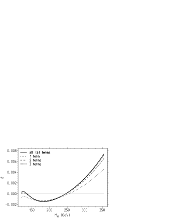
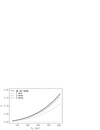
Figure 4: The dependence on the number of coefficients of the expansion with respect to $\sin^{2}\theta_{W}$ of the two–loop corrections $\delta\equiv\Biggl{\{}\Pi_{Z}^{(2)}+\Pi_{Z}^{(1)}\Pi_{Z}^{(1)}{}^{\prime}\Biggr{\}}_{\overline{\rm MS}}$ (see 4.66) as a function of the Higgs mass. The dotted, dashed, dot-dashed and full lines show results obtained with the first one, two, three and all calculated (six) coefficients, respectively. Upper plot: for intermediate Higgs masses. Lower plot: for heavy Higgs masses.

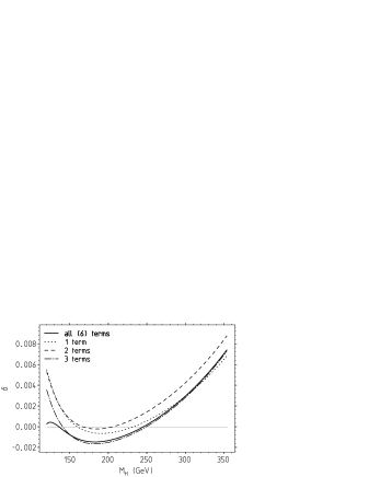
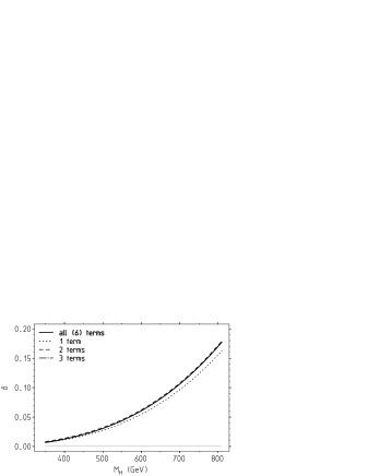
Figure 5: The dependence on the number of coefficients of the expansion with respect to $m^{2}_{Z}/m^{2}_{i}$ ($i=H,t$) used for the evaluation of the two-loop corrections. We show $\delta\equiv\Biggl{\{}\Pi_{Z}^{(2)}+\Pi_{Z}^{(1)}\Pi_{Z}^{(1)}{}^{\prime}\Biggr{\}}_{\overline{\rm MS}}$ (see 4.66) as a function of the Higgs mass. The dotted, dashed, dot-dashed and full lines show results obtained with the first one, two, three and all calculated (six) coefficients, respectively. Upper plot: for intermediate Higgs masses. Lower plot: for heavy Higgs masses.

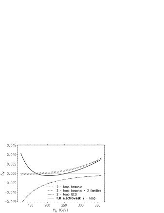
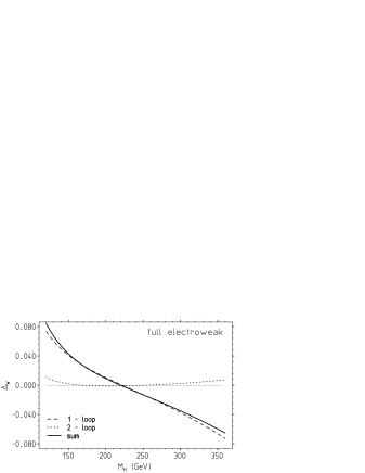
Figure 6: Corrections to the relation $\Delta_{W}\equiv M^{2}_{W}/m^{2}_{W}(M_{W})-1$ as a function of the Higgs mass $M_{H}$ for intermediate Higgs masses. Upper plot: the various two-loop corrections. Lower plot: the complete one- and two-loop correction.

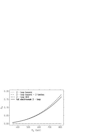
Figure 8: Corrections to the relation $\Delta_{W}\equiv M^{2}_{W}/m^{2}_{W}(M_{W})-1$ as a function of the Higgs mass $M_{H}$ for heavy Higgs masses. Upper plot: the various two-loop corrections. Lower plot: the complete one- and two-loop correction.

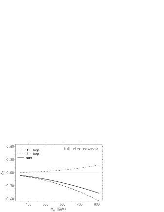
Figure 9: Corrections to the relation $\Delta_{Z}\equiv M^{2}_{Z}/m^{2}_{Z}(M_{Z})-1$ as a function of the Higgs mass $M_{H}$ for heavy Higgs masses. Upper plot: the various two-loop corrections. Lower plot: the complete one- and two-loop correction.

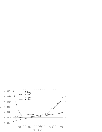
Figure 10: Two–loop imaginary part $\delta={\rm Im}s_{P,\>V}/m_{V}^{2}$ (imag) and absolute value $\delta=|s_{P,\>V}|/m_{V}^{2}$ (abs) of the pole position $s_{P}$ for the $Z$ (Z) and the $W$ (W) as a function of the Higgs mass $M_{H}$. Upper plot: for intermediate Higgs masses. Lower plot: for heavy Higgs masses.

The general features of our expansion have been discussed in I. While the series expansion in $\sin^{2}\theta_{W}$ for the known fixed value converges very well, the expansions in $M_{V}^{2}/m_{H}^{2}$ for large $m_{H}$ leads to a strong coupling problem and perturbation theory becomes useless above about 800 GeV. In general, as is illustrated by Figs. 4 and 5, the first three coefficients yield a good approximation as long as the asymptotic series behaves well. Of course, the expansion in $M_{V}^{2}/m_{H}^{2}$ for smaller values of $m_{H}$ starts to diverge below about 120 GeV. We have calculated six terms in each of the different expansion parameters, but only write down three of them in Appendix E . Figs. 6–9 show the corrections $\Delta_{W}\equiv M^{2}_{W}/m^{2}_{W}(M_{W})-1$ and $\Delta_{Z}\equiv M^{2}_{Z}/m^{2}_{Z}(M_{Z})-1$, respectively, as a function of the Higgs mass $M_{H}$ for intermediate and for heavy Higgs masses. The light fermion contributions are small relative to the other corrections. The same is true for the QCD corrections for Higgs masses above about 300 GeV. In Fig. 10 the imaginary part and the absolute value of the pole position $s_{P}$ are shown.

Very often the inverse of (5.1) is required. To that end we have to solve the real part of (2.3) iteratively for $m_{V}^{2}$ and to express all $\overline{\rm MS}$ parameters in terms of on-shell ones.

The solution to two loops reads

$$m^{2}_{V} = M_{V}^{2}-{\rm Re}\hat{\Pi}_{V}^{(1)}-{\rm Re}\Biggl{\{}\Pi_{V}^{(2)}+\Pi_{V}^{(1)}\Pi_{V}^{(1)}{}^{\prime}\Biggr{\}}_{\overline{\rm MS}}$$ (5.2)

$$-\sum\limits_{j}(\Delta m^{2}_{j})^{(1)}\frac{\partial}{\partial m_{j}^{2}}{\rm Re}\hat{\Pi}_{V}^{(1)}-(\Delta e)^{(1)}\frac{\partial}{\partial e}{\rm Re}\hat{\Pi}_{V}^{(1)}\Biggr{|}_{m_{j}^{2}=M_{j}^{2},\,e=e_{\rm OS}},$$

where the sum runs over all species of particles $j=Z,\,W,\,H,\,t$ and

$$(\Delta m^{2}_{j})^{(1)}=-{\rm Re}\hat{\Pi}^{(1)}_{j}\Biggr{|}_{m_{j}^{2}=M_{j}^{2},\,e=e_{\rm OS}}\equiv-M_{V}^{2}\frac{e^{2}_{\rm OS}}{16\pi^{2}\sin^{2}\theta_{W}}X_{V}^{(1)}\Biggr{|}_{m_{j}^{2}=M_{j}^{2}}$$

stands for the self-energy of the $j$th particle at $p^{2}=m_{j}^{2}$ in the $\overline{\rm MS}$ scheme and parameters replaced by the on-shell ones. The analytical results for the derivative term $\sum\limits_{j}\delta_{j}\frac{\partial}{\partial m_{j}^{2}}\hat{\Pi}_{V}^{(1)}$ can be extracted from the results of Appendix C. In (5.2) $m^{2}_{V}-M_{V}^{2}=\left(\delta M_{V}^{2}\right)_{\rm finite}$ represents the finite part of the on–shell mass counter–term. The corresponding bare one is obtained by adding the $\overline{\rm MS}$ mass counter–term (see section 4.2) $\delta m_{V}^{2}=\left(Z_{\overline{MS}}-1\right)m_{V}^{2}=m_{0V}^{2}-m_{V}^{2}$.

The relation (5.2) involves a change from the $\overline{\rm MS}$ to the on-shell (OS) scheme also for the electric charge. Let us consider therefore, in details, the relationship between the fine structure constants $\alpha_{\overline{\rm MS}}$ and $\alpha_{\rm OS}=\alpha$.

For the electroweak couplings we have to calculate the $\overline{\rm MS}$ versions from their commonly used on-shell values. The $\overline{\rm MS}$ version of the fine structure constant is defined as a solution of the renormalization group equation (see 4.46) and can be calculated from the UV-counterterms of the electrical charge $e$ (see (4.45)). In perturbation theory the naive relation between $\overline{\rm MS}$ and on-shell values of $\alpha$ is determined by the Thomson limit of Compton scattering and can be written as

$$\alpha(\mu^{2}) = \alpha\Biggl{\{}1+\frac{\alpha}{4\pi}\Biggl{[}7\ln\left(\frac{m_{W}^{2}}{\mu^{2}}\right)-\frac{2}{3}+\frac{4}{3}\sum Q_{f}^{2}N_{cf}\ln\frac{\mu^{2}}{m_{f}^{2}}\Biggr{]}\Biggr{\}}\;,$$ (5.3)

where the sum goes over all fermions $f$ with $N_{cf}=1$ for leptons and $N_{cf}=3$ for quarks and $Q_{f}$ is the fermion charge equal to 1 for leptons, -1/3 and 2/3 for d- and u-quarks, correspondingly.

The terms proportional to logarithms of the fermion masses originate from evaluating the finite part of the derivative of the photon propagator at zero momentum transfer, which we denote as $\Pi^{f}_{\gamma\gamma}(0)$. However, the low energy contribution of the five light quarks $(u,d,s,c,b)$ cannot be calculated in perturbation theory. The free quark loops are strongly (non-perturbatively) modified by the strong interaction at low energies. In order to evaluate $\Pi^{f}_{\gamma\gamma}(0)$ we may write it as

$$\Pi^{f}_{\gamma\gamma}(0)={\rm Re}\Pi^{f}_{\gamma\gamma}(q^{2})-\Biggl{[}{\rm Re}\Pi^{f}_{\gamma\gamma}(q^{2})-\Pi^{f}_{\gamma\gamma}(0)\Biggr{]}\;,$$ (5.4)

where $q^{2}$ is chosen sufficiently large (typically $M_{Z}^{2}$) such that the first term on the r.h.s. can be calculated in perturbative QCD. In the limit of large momentum transfer $s\gg m_{f}^{2}$ the result is

$${\rm Re}\Pi^{f}_{\gamma\gamma}(s)=\frac{4}{3}\sum_{f}Q_{f}^{2}N_{cf}\left(\ln\frac{s}{\mu^{2}}-\frac{5}{3}\right)\;,$$ (5.5)

which we use in the relation (5.3) for the perturbative light quarks contributions $(s=M_{Z}^{2})$.

On the grounds of analyticity and unitarity, the second non–perturbative term in (5.4) can be determined by evaluating a dispersion integral over the known experimental $e^{+}e^{-}\to{\rm hadrons}$ cross–section (for details see [53]). Usually, the cross–sections are represented in terms of the cross–section ratio

$$R(s)=\frac{\sigma_{tot}(e^{+}e^{-}\to\gamma^{*}\to{\rm hadrons})}{\sigma(e^{+}e^{-}\to\gamma^{*}\to\mu^{+}\mu^{-})}\;,$$

where $\sigma(e^{+}e^{-}\to\gamma^{*}\to\mu^{+}\mu^{-})=\frac{4\pi\alpha^{2}}{3s}$ at tree level. In terms of $R(s)$ we obtain

$$\Delta\Pi_{\gamma\gamma}(q^{2})\equiv\Biggl{[}{\rm Re}\Pi_{\gamma\gamma}(q^{2})-\Pi_{\gamma\gamma}(0)\Biggr{]}=-\frac{4q^{2}}{3}\int_{4m_{\pi}^{2}}^{\infty}ds\frac{R(s)}{s\>(s-q^{2}-i\epsilon)}.$$

The shift in the fine structure constant in then $\Delta\alpha(s)=4\pi\alpha\times\frac{1}{16\pi^{2}}\Delta\Pi_{\gamma\gamma}(s)$. Using the experimental data for $R(s)$ up to $\sqrt{s}=E_{cut}=5$ GeV and for the $\Upsilon$ resonances region between 9.6 and 13 GeV and perturbative QCD from 5.0 to 9.6 GeV and for the high energy tail above 13 GeV one gets

$$\Delta\alpha_{\rm hadrons}^{(5)}(M^{2}_{Z}) = 0.027572\pm 0.000359\;\;;\;\;\;\alpha^{-1}(M_{Z}^{2})=128.952\pm 0.049$$ (5.6)

at $M_{Z}=$ 91.19 GeV. For numerical estimations we use the results of [54].

The shift in $\alpha$ calculated by the dispersion relation corresponds to the on-shell scheme. Accordingly, since $\hat{\Pi}^{(1)}$ depends on $e$ by an overall factor $e^{2}$ only, we have

$$(\Delta e)^{(1)}\frac{\partial}{\partial e}\hat{\Pi}_{V}^{(1)}=\left\{\delta\alpha_{\rm bos}+\delta\alpha_{\rm lep}+\delta\alpha_{\rm top}+\Delta\alpha_{\rm hadrons}^{(5)}(M^{2}_{Z})-\delta\Delta\alpha_{\rm udscb}(M^{2}_{Z})\right\}\hat{\Pi}_{V}^{(1)}\;,$$

where

$$\delta\alpha_{\rm bos}=\frac{\alpha}{4\pi}\left(7\ln\frac{M_{W}^{2}}{\mu^{2}}-\frac{2}{3}\right),\;\;\delta\alpha_{\rm lep}=-\frac{\alpha}{3\pi}\sum\limits_{\ell=e,\mu,\tau}\ln\frac{m^{2}_{\ell}}{\mu^{2}},\;\;\delta\alpha_{\rm top}=-\frac{4\alpha}{9\pi}\ln\frac{m^{2}_{t}}{\mu^{2}}$$

and

$$\delta\Delta\alpha_{\rm udscb}(M^{2}_{Z})=\frac{11\alpha}{9\pi}\left(\ln\frac{M_{Z}^{2}}{\mu^{2}}-\frac{5}{3}\right)$$

the perturbative subtraction-term (5.5) form the 5 light quarks. The quark loops contributing to the on–shell gauge boson self–energies are evaluated here at a high energy scale and hence it should be save to calculate them in perturbation theory.

Finally, we analyze the Higgs mass dependence of the $\overline{\rm MS}$ parameter $\sin^{2}\theta$ defined as

$$\sin^{2}\theta_{W}=1-\frac{m_{W}^{2}}{m_{Z}^{2}}=\frac{g^{\prime 2}}{g^{2}+g^{\prime 2}}.$$ (5.7)

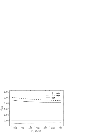
Figure 11: One- and two-loop corrections to $\delta_{\sin^{2}\Theta}=\sin^{2}\theta^{\overline{\rm MS}}_{W}/\sin^{2}\theta^{\rm OS}_{W}-1$ (see (5.7)) as a function of the Higgs mass $m_{H}$ ($\mu=M_{Z}$).

The Fig. 11 shows the correction to $\delta_{\sin^{2}\Theta}=\sin^{2}\theta^{\overline{\rm MS}}_{W}/\sin^{2}\theta^{\rm OS}_{W}-1$ as a function of the Higgs mass. Since the unphysical $m_{H}^{4}$ terms drop out by virtue of Veltman’s screening theorem, the corrections do not blow up so dramatically in the strong coupling regime of large Higgs masses. In the region displayed between 150 and 800 GeV the two–loop correction stays below about 0.6% and has a sign opposite to the one–loop correction. The latter is one order of magnitude larger.

6 Conclusion

We have calculated the full SM two–loop radiative corrections to the pole masses of the gauge bosons $W$ and $Z$. A number of conceptual problems dealing with the renormalization of unstable particles could be studied by explicite calculations: i) The position of the complex pole $s_{P}$ of the gauge boson propagators is manifestly gauge invariant after taking into account the Higgs tadpole contributions. ii) The renormalized on-shell self–energies are infrared finite. iii) Our calculation proves that the $\overline{\rm MS}$ renormalization scheme, comprised in (4.66), is self consistent and works properly in case of unstable particles. iv) Up to two–loops we explicitely confirm that the UV singularities and the related RG equations of the broken phase are completely determined by the unbroken phase [45]. v) The inclusion of the tadpoles is also required from the point of view of the renormalization group invariance. vi) Our results for the 2-loop mass renormalization constants in the on-shell and the $\overline{\rm MS}$ scheme can be applied in calculations of physical quantities in both of these schemes at the 2-loop level. vi) A compact expression for the massless fermion contributions in terms of an irreducible set of master–integrals in given. vii) A new technique for calculating the $\varepsilon$–expansion of some types of hypergeometric functions has been developed.

Note that all results concerning general properties (like gauge invariance etc.) have been checked analytically. Since exact analytical results for many of the multi–scale master–integrals are not yet available, in this work we had to resort to asymptotic expansion techniques. The exact results in terms of a basis of master–integrals will by given elsewhere. For the latter one dimensional integral representations are available which are suitable for the numerical evaluations [10]. However, for numerical evaluations in the heavy Higgs region above about 200 GeV, the computation in terms of our series expansions is numerically much more stable and much more efficient.

Acknowledgments. We are grateful to D. Bardin, A. Davydychev, O. V. Tarasov and B. Tausk for useful discussions. M. K.’s research was supported in part by INTAS-CERN grant No. 99-0377 and by the Australian Research Council grant No. A00000780. We thank Oleg Tarasov for carefully reading the manuscript.

Appendix

Appendix A Sums with binomial coefficients in the numerator

Let us present in the following some useful formulae for the binomial sums which occur in the master-integrals (3.38) and (3.40). The sums which involve only harmonic coefficients, were investigated in [55], while the sums with binomial coefficients in the denominator were considered in [25, 56]. In this Appendix we present some results for sums with binomial coefficients in the numerator. A sum $F_{a}$ of weight $a$ has form

$$F_{a}(x)\equiv\sum_{k=1}^{\infty}\left(2k\atop k\right)f(k)\frac{x^{k}}{k^{a}}$$ (A.1)

where $f(k)$ is a product of some finite sums (e.g. $S_{a},\bar{S}_{b}$, etc.). It is convenient to introduce a new variable $\chi$ related to $x$ via

$$\chi = \frac{1-\sqrt{1-4x}}{1+\sqrt{1-4x}},~{}~{}~{}~{}x=\frac{\chi}{(1+\chi)^{2}},~{}~{}~{}~{}\sqrt{1-4x}=\frac{1-\chi}{1+\chi}.$$ (A.2)

A general relation for sums of type (A.1) is then given by

$$F_{a-1}(x)=x\frac{d}{dx}F_{a}(x)=\frac{1+\chi}{1-\chi}\chi\frac{d}{d\chi}\tilde{F}_{a}(\chi).$$ (A.3)

Relevant analytical results for sums of the type considered are:

$$\sum\limits_{k=1}^{\infty}\left(2k\atop k\right)\frac{x^{k}}{k^{4}}=-8{\mbox{S}}_{1,2\!}\left(-\chi\right)\ln(1+\chi)+4{\mbox{Li}}_{3}\left(-\chi\right)\ln(1+\chi)-4{\mbox{Li}}_{2}\left(-\chi\right)\ln^{2}(1+\chi)$$

$$\hskip 85.35826pt-\frac{2}{3}\ln^{4}(1+\chi)-{\mbox{Li}}_{4}\left(-\chi\right)+4{\mbox{S}}_{2,2\!}\left(-\chi\right)-8{\mbox{S}}_{1,3\!}\left(-\chi\right),$$ (A.4)

$$\sum_{k=1}^{\infty}\left(2k\atop k\right)\frac{x^{k}}{k^{2}}S_{1}=-\frac{4}{3}\ln^{3}(1+\chi)+\frac{1}{2}{\mbox{Li}}_{3}\left(\chi^{2}\right)-2\ln(1+\chi){\mbox{Li}}_{2}\left(\chi^{2}\right)$$

$$\hskip 85.35826pt+4{\mbox{S}}_{1,2\!}\left(\chi\right)-2{\mbox{S}}_{1,2\!}\left(\chi^{2}\right),$$ (A.5)

$$\sum_{k=1}^{\infty}\left(2k\atop k\right)\frac{x^{k}}{k^{2}}\bar{S}_{1}=-\frac{2}{3}\ln^{3}(1+\chi)+2{\mbox{Li}}_{3}\left(\chi\right)-4\ln(1+\chi){\mbox{Li}}_{2}\left(\chi\right)$$

$$\hskip 85.35826pt+4{\mbox{S}}_{1,2\!}\left(\chi\right)+6{\mbox{S}}_{1,2\!}\left(-\chi\right)-2{\mbox{S}}_{1,2\!}\left(\chi^{2}\right),$$ (A.6)

$$\sum_{k=1}^{\infty}\left(2k\atop k\right)\frac{x^{k}}{k}S_{2}=-\frac{4}{3}\ln^{3}(1+\chi)-4\ln(1+\chi){\mbox{Li}}_{2}\left(-\chi\right)-4{\mbox{S}}_{1,2\!}\left(-\chi\right),$$ (A.7)

$$\sum_{k=1}^{\infty}\left(2k\atop k\right)\frac{x^{k}}{k}S_{1}^{2}=\frac{4}{3}\ln^{3}(1+\chi)+8\ln(1+\chi){\mbox{Li}}_{2}\left(\chi\right)+4\ln(1+\chi){\mbox{Li}}_{2}\left(-\chi\right)$$

$$\hskip 85.35826pt-4{\mbox{S}}_{1,2\!}\left(-\chi\right)+4{\mbox{S}}_{1,2\!}\left(\chi^{2}\right),$$ (A.8)

$$\sum_{k=1}^{\infty}\left(2k\atop k\right)\frac{x^{k}}{k}S_{1}\bar{S}_{1}=\frac{2}{3}\ln^{3}(1+\chi)+6\ln(1+\chi){\mbox{Li}}_{2}\left(\chi\right)-6{\mbox{S}}_{1,2\!}\left(-\chi\right)$$

$$\hskip 85.35826pt+4{\mbox{S}}_{1,2\!}\left(\chi\right)+2{\mbox{S}}_{1,2\!}\left(\chi^{2}\right),$$ (A.9)

$$\sum_{k=1}^{\infty}\left(2k\atop k\right)\frac{x^{k}}{k}\Biggl{[}\bar{S}_{2}-\bar{S}_{1}^{2}\Biggr{]}=-\frac{2}{3}\ln^{3}(1+\chi)-4\ln(1+\chi){\mbox{Li}}_{2}\left(\chi\right)-8{\mbox{S}}_{1,2\!}\left(\chi\right)\;,$$ (A.10)

$$\sum_{k=1}^{\infty}\left(2k\atop k\right)\frac{x^{k}}{k}V_{2}=-{\mbox{Li}}_{3}\left(\chi\right)-2{\mbox{Li}}_{3}\left(-\chi\right)+\frac{1}{9}{\mbox{Li}}_{3}\left(\chi^{3}\right)-{\mbox{Li}}_{3}\left(x\right).$$ (A.11)

All these low-weights sums may be obtained by applying (A.3).

The following representation is often useful for sums of the type just considered:

$$\sum_{n=1}^{\infty}\left(2n\atop n\right)\frac{x^{n}}{n^{a}}f(n)=\frac{1}{(a-2)!}\int_{0}^{x}\sum_{n=1}^{\infty}\left(2n\atop n\right)\frac{z^{n}}{n}f(n)\Biggl{[}\ln x-\ln z\Biggr{]}^{a-2}\frac{dz}{z}\;,$$ (A.12)

where $f(n)$ is an arbitrary combination of finite sums. For particular cases, $f(n)=1,S_{1},\bar{S}_{1},$ $S_{2},S_{1}\bar{S}_{1},\bar{S}_{2}-\bar{S}_{1}^{2}$ or $V_{2}$, the corresponding expressions extracted from (A)-(A.11) allow us to perform the sum under the integral in (A.12) exactly and to obtain one-fold integral representations for a large class of binomial sums. For $0\leq x\leq 1/4$ , a further simplification is possible by substituting, $z=\frac{1}{4}\sin^{2}\phi$. It leads to the following representation:

$$\sum_{n=1}^{\infty}\left(2n\atop n\right)\frac{x^{n}}{n^{a}}f(n) = \frac{2}{(a-2)!}\int_{0}^{\arcsin\sqrt{4x}}d\phi\frac{\cos\phi}{\sin\phi}\Biggl{[}\ln(4x)-\ln(\sin^{2}\phi)\Biggr{]}^{a-2}\times$$ (A.13)

$$\sum_{n=1}^{\infty}\left(2n\atop n\right)\frac{f(n)}{n}\left(\frac{\sin^{2}\phi}{4}\right)^{n}$$

$$\equiv \Sigma(f,\arcsin\sqrt{4x})~{}~{},$$

where $\Sigma(f,\theta)$ is the short notation for this sum. Unfortunately, we could not find corresponding analytical results for these sums for arbitrary $x\;(x\leq 1/4)$ in terms of known functions, like generalized Nielsen polylogarithms. Not even for the simplest case $f(n)=1$, which yields

$$\sum_{n=1}^{\infty}\left(2n\atop n\right)\frac{x^{n}}{n^{a}} = -\frac{2^{a+1}}{(a-2)!}\int_{0}^{\arcsin\sqrt{4x}}\ln\left(\cos\frac{\theta}{2}\right)\Biggl{[}\ln(2\sqrt{x})-\ln\left(\sin\theta\right)\Biggr{]}^{a-2}d\Biggl{(}\ln\sin\theta\Biggr{)}\;,$$

a solution could be found. The problem here may be compared with the one encountered in the context of the inverse binomial sums, considered in [56, 57].

For $x>1/4$ the representation

$$\sum_{n=1}^{\infty}\left(2n\atop n\right)\frac{x^{n}}{n^{a}}f(n) = \Sigma\left(f,\frac{\pi}{2}\right)+\frac{1}{(a-2)!}\int_{\frac{1}{4}}^{x}\sum_{n=1}^{\infty}\left(2n\atop n\right)\frac{z^{k}}{n}f(n)\Biggl{[}\ln x-\ln z\Biggr{]}^{a-2}\frac{dz}{z}$$ (A.14)

$$= \Sigma\left(f,\frac{\pi}{2}\right)+\frac{2^{a-2}}{(a-2)!}\int_{0}^{2\arccos\frac{1}{\sqrt{4x}}}d\theta\frac{\sin\frac{\theta}{2}}{\cos\frac{\theta}{2}}\Biggl{[}\ln\sqrt{x}+\ln\left(2\cos\frac{\theta}{2}\right)\Biggr{]}^{a-2}\times$$

$$\hskip 85.35826pt\sum_{n=1}^{\infty}\left(2n\atop n\right)\frac{f(n)}{n}\left(\frac{1}{4\cos^{2}\frac{\theta}{2}}\right)^{n}$$

is available, where we have introduced a new variable $z=1/(4\cos^{2}\frac{\theta}{2})$ and $\Sigma\left(f,\frac{\pi}{2}\right)$ is a constant, related to some (combination of) hypergeometric functions ${}_{P}F_{Q}$ of argument unity. For each given choice of $f(n)$ these constants are different, but in all cases they are expressible in terms of “even basis” elements (see [58] and Appendix B.1 in [37]). We have checked this statement by high-precision calculations, which allow for “numerical proofs” in the manner explained in [56]. The second term of (A.14) can be calculated analytically for some particular cases. For example, for $f(n)=1$ we have

$$\sum_{n=1}^{\infty}\left(2n\atop n\right)\frac{x^{n}}{n^{a}} = \frac{1}{2}~{}{}_{a+2}F_{a+1}\left(\begin{array}[]{c|}{\textstyle{\frac{3}{2}}},\{1\}_{a+1}\\ \{2\}_{a+1}\end{array}~{}1\right)-\frac{2^{a}}{(a-2)!}\sum_{j=0}^{a-2}\left(a-2\atop j\right)\left(\ln\sqrt{x}\right)^{a-2-j}\times$$

$$\Biggl{\{}\frac{1}{j+2}\Biggl{[}\ln^{j+2}\left(2\cos\frac{\theta}{2}\right)-\ln^{j+2}2\Biggr{]}$$

$$+\frac{\mbox{i}\sigma}{2(j+1)}\Biggl{[}{\mbox{Ls}}_{j+2}\left(\pi-\theta\right)-{\mbox{Ls}}_{j+2}\left(\pi\right)-\theta\ln^{j+1}\left(2\cos\frac{\theta}{2}\right)\Biggr{]}\Biggr{\}}\;,$$

where we have used $\sum\limits_{k=1}^{\infty}\left(2k\atop k\right)\frac{x^{k}}{k}=2\ln(1+\chi)$, $a\geq 2$, $\theta=2\arccos\frac{1}{\sqrt{4x}}\,,$ $\sigma=\pm 1$ and ${\mbox{Ls}}_{n}\left(\theta\right)$ is so-called log-sine integral [32] defined by

$${\mbox{Ls}}_{j}^{(k)}\left(\theta\right)=-\int\limits_{0}^{\theta}{\rm d}\phi\;\phi^{k}\ln^{j-k-1}\left|2\sin\frac{\phi}{2}\right|\,,~{}~{}~{}{\mbox{Ls}}_{j}\left(\theta\right)\equiv{\mbox{Ls}}_{j}^{(0)}\left(\theta\right)\;.$$ (A.19)

The values of ${\mbox{Ls}}_{j}\left(\pi\right)$ can be expressed in terms of $\zeta$–function for any $j$ [32]. The sign $\sigma$ is defined via the relation $\chi\equiv e^{-{\rm i}\sigma\theta}$. The choice of the sign derives from the causal “+i0”–prescription for the propagator or as the sign of the square root of $\cos^{2}\frac{\theta}{2}$. In the physical region of interest here we have $\sigma=-1$.

For $x>1/4$, an non–zero imaginary part develops for the sum (LABEL:f=1). It can be calculated in closed form:

$${\it Im}\sum_{n=1}^{\infty}\left(2n\atop n\right)\frac{x^{n}}{n^{a}} = -\sigma\frac{2^{a-1}}{(a-2)!}\sum_{j=0}^{a-2}\left(a-2\atop j\right)\frac{\left(\ln\sqrt{x}\right)^{a-2-j}}{j+1}\times$$

$$\Biggl{[}{\mbox{Ls}}_{j+2}\left(\pi-\theta\right)-{\mbox{Ls}}_{j+2}\left(\pi\right)-\theta\ln^{j+1}\left(2\cos\frac{\theta}{2}\right)\Biggr{]}_{\theta=2\arccos\frac{1}{\sqrt{4x}}}.$$

On the mass–shell $(x=1,\theta=\frac{2\pi}{3},\sigma=-1)$ we find the result

$$\sum_{n=1}^{\infty}\left(2n\atop n\right)\frac{1}{n^{a}} = \frac{1}{2}~{}{}_{a+2}F_{a+1}\left(\begin{array}[]{c|}{\textstyle{\frac{3}{2}}},\{1\}_{a+1}\\ \{2\}_{a+1}\end{array}~{}1\right)+\frac{2^{a}}{(a-2)!}\frac{\ln^{a}2}{a}$$ (A.24)

$$+\mbox{i}\frac{2^{a-1}}{(a-1)!}\Biggl{[}{\mbox{Ls}}_{a}\left(\frac{\pi}{3}\right)-{\mbox{Ls}}_{a}\left(\pi\right)\Biggr{]}.$$

In general, however, analytical results for these types of sums are not expressible in terms of generalized Nielsen polylogarithms. For example, we have

$$\sum_{n=1}^{\infty}\left(2n\atop n\right)\frac{x^{n}}{n^{a}}\bar{S}_{1}=\Sigma\left(\bar{S}_{1},\frac{\pi}{2}\right)+\frac{2^{a-2}}{(a-2)!}\int_{0}^{2\arccos\frac{1}{\sqrt{4x}}}d\theta\frac{\sin\frac{\theta}{2}}{\cos\frac{\theta}{2}}\Biggl{[}\ln\sqrt{x}+\ln\left(2\cos\frac{\theta}{2}\right)\Biggr{]}^{a-2}\times$$

$$\hskip 85.35826pt\Biggl{\{}\Biggl{[}2\zeta_{2}-\pi\theta+\frac{\theta^{2}}{4}+\ln^{2}\left(2\cos\frac{\theta}{2}\right)\Biggr{]}-\mbox{i}\Biggl{[}2{\mbox{Cl}}_{2}\left(\theta\right)+\theta\ln\left(2\cos\frac{\theta}{2}\right)\Biggr{]}\Biggr{\}}$$

$$=\Sigma\left(\bar{S}_{1},\frac{\pi}{2}\right)-\frac{2^{a-1}}{(a-2)!}\sum_{j=0}^{a-2}\left(a-2\atop j\right)\frac{\left(\ln\sqrt{x}\right)^{a-2-j}}{j+1}\times$$

$$\Biggl{\{}\Biggl{[}2\zeta_{2}-\pi\theta+\frac{\theta^{2}}{4}\Biggr{]}\ln^{j+1}\left(2\cos\frac{\theta}{2}\right)+\frac{\pi}{2}\Biggl{[}{\mbox{Ls}}_{j+2}\left(\pi-\theta\right)-{\mbox{Ls}}_{j+2}\left(\pi\right)\Biggr{]}-2\zeta_{2}\ln^{j+1}2$$

$$+\frac{1}{2}\Biggl{[}{\mbox{Ls}}_{j+3}^{(1)}\left(\pi-\theta\right)-{\mbox{Ls}}_{j+3}^{(1)}\left(\pi\right)\Biggr{]}+\frac{j+1}{j+3}\Biggl{[}\ln^{j+3}\left(2\cos\frac{\theta}{2}\right)-\ln^{j+3}2\Biggr{]}$$

$$-2\mbox{i}\sigma\Biggr{[}{\mbox{Cl}}_{2}\left(\theta\right)\ln^{j+1}\left(2\cos\frac{\theta}{2}\right)-{\mbox{Lsc}}_{2,j+2\!}\left(\theta\right)\Biggl{]}$$

$$-\mbox{i}\sigma\frac{j+1}{j+2}\Biggl{[}{\mbox{Ls}}_{j+3}\left(\pi\right)-{\mbox{Ls}}_{j+3}\left(\pi-\theta\right)+\theta\ln^{j+2}\left(2\cos\frac{\theta}{2}\right)\Biggr{]}\Biggr{\}}_{\theta=2\arccos\frac{1}{\sqrt{4x}}}\;,$$ (A.25)

where $\sum\limits_{k=1}^{\infty}\left(2k\atop k\right)\frac{x^{k}}{k}\bar{S}_{1}=2{\mbox{Li}}_{2}\left(\chi\right)+\ln^{2}(1+\chi)$ and ${\mbox{Lsc}}_{i,j\!}\left(\theta\right)$ are new type of log-sine integrals introduced in [37] (where the properties of these functions are given in Appendix A.2) and defined by

$${\mbox{Lsc}}_{i,j\!}\left(\theta\right)=-\int\limits_{0}^{\theta}{\mbox{d}}\phi\ln^{i-1}\left|2\sin\frac{\phi}{2}\right|\ln^{j-1}\left|2\cos\frac{\phi}{2}\right|\;.$$ (A.26)

For $i,j>2$ these functions cannot be written in terms of Nielsen polylogarithms, but are related to harmonic polylogarithms which have been considered in [59].

Using the results for the binomial series given above, we are able to calculate analytically the required first few coefficients of the $\varepsilon$–expansion of hypergeometric functions of the following type

$${}_{Q}F_{P}\left(\begin{array}[]{c|}{\textstyle{\frac{3}{2}}}+b_{1}\varepsilon,\ldots,{\textstyle{\frac{3}{2}}}+b_{I}\varepsilon,\;1+a_{1}\varepsilon,\ldots,1+a_{K}\varepsilon,\;2+d_{1}\varepsilon\ldots,2+d_{L}\varepsilon\\ {\textstyle{\frac{3}{2}}}+f_{1}\varepsilon,\ldots,{\textstyle{\frac{3}{2}}}+f_{J}\varepsilon,\;1+e_{1}\varepsilon,\ldots,1+e_{R}\varepsilon,\;2+c_{1}\varepsilon,\ldots,2+c_{Q-J-R}\varepsilon\end{array}~{}z\right)\;.$$ (A.27)

Rewriting this function as an infinite series and using the well-know representation

$$\frac{\Gamma(j+a\varepsilon)}{\Gamma(1+a\varepsilon)}=(j-1)!\;\exp\left[-\sum_{k=1}^{\infty}\frac{(-a\varepsilon)^{k}}{k}S_{k}(j-1)\right]\;,$$

we obtain (for details we refer to Appendix B of [37])

$${}_{P+1}F_{P}\left(\begin{array}[]{c|}\{{\textstyle{\frac{3}{2}}}+b_{i}\varepsilon\}_{0}^{J+1},\;\{1+a_{i}\varepsilon\}_{0}^{K},\;\{2+d_{i}\varepsilon\}_{0}^{L}\\ \{{\textstyle{\frac{3}{2}}}+f_{i}\varepsilon\}_{0}^{J},\;\{1+e_{q}\varepsilon\}_{0}^{R},\{2+c_{i}\varepsilon\}_{0}^{K+L-R}\end{array}~{}4z\right)=\frac{1}{2z}\times$$ (A.30)

$$\Pi_{s=1}^{K+L-R}(1+c_{s}\varepsilon)\Pi_{i=1}^{L}\frac{1}{(1+d_{i}\varepsilon)}\Pi_{r=1}^{J+1}\frac{1}{(1+2b_{r}\varepsilon)}\Pi_{k=1}^{J}(1+2f_{k}\varepsilon)\sum_{j=1}^{\infty}\left(2j\atop j\right)\frac{z^{j}}{j^{K-R-1}}\times\Delta\;,$$

(A.31)

where $P=K+L+J$ and

$$\Delta=\exp\left(\sum_{k=1}^{\infty}\frac{(-\varepsilon)^{k}}{k}\left\{S_{k}T_{k}+2^{k}U_{k}\bar{S}_{k}+\frac{Y_{k}}{j^{k}}\right\}\right)=\Biggl{(}1-\varepsilon\left\{S_{1}T_{1}+\frac{Y_{1}}{j}+2U_{1}\bar{S}_{1}\right\}$$

$$+\varepsilon^{2}\Biggl{\{}\frac{1}{2j^{2}}\left[Y_{2}+Y_{1}^{2}\right]+\frac{Y_{1}}{j}\left[S_{1}T_{1}+2U_{1}\bar{S}_{1}\right]+2U_{1}S_{1}\bar{S}_{1}T_{1}+2U_{2}\bar{S}_{2}+2U_{1}^{2}\bar{S}_{1}^{2}$$

$$~{}~{}~{}~{}~{}~{}+\frac{1}{2}S_{2}T_{2}+\frac{1}{2}S_{1}^{2}T_{1}^{2}\Biggr{\}}+{\rm O}(\varepsilon^{3})\Biggr{)}\;.$$ (A.32)

Here, we introduced new constants $A_{k},B_{k},C_{k},D_{k},E_{k},F_{k},T_{k},U_{k}$: $A_{k}\equiv\sum_{i=1}^{K}a_{i}^{k}$, $B_{k}\equiv\sum_{i=1}^{J-1}b_{i}^{k}$, $C_{k}\equiv\sum_{i=1}^{K+L-R-2}c_{i}^{k}$, $D_{k}\equiv\sum_{i=1}^{L}d_{i}^{k}$, $E_{k}\equiv\sum_{i=1}^{R}e_{i}^{k}$, $F_{k}\equiv\sum_{i=1}^{J}f_{i}^{k}$, $T_{k}\equiv B_{k}+C_{k}+E_{k}-A_{k}-D_{k}-F_{k}$, $U_{k}\equiv F_{k}-B_{k}$, $Y_{k}\equiv C_{k}-D_{k}$. With the expansion just worked out, analytical results are available for the first three coefficients of the $\varepsilon$–expansion of the hypergeometric function (A.27). In particular, we find

$${}_{2}F_{1}\left(\begin{array}[]{c|}{\textstyle{\frac{3}{2}}}-2\varepsilon\;,1\\ 2-3\varepsilon\end{array}~{}4z\right)=\frac{1}{2z}\frac{1-3\varepsilon}{1-4\varepsilon}\frac{1+\chi}{1-\chi}\Biggl{[}\frac{2\chi}{1+\chi}-2\Biggl{\{}\ln(1-\chi)+2\ln(1+\chi)\Biggr{\}}\varepsilon$$ (A.35)

$$+2\varepsilon^{2}\Biggl{\{}3\Biggl{(}{\mbox{Li}}_{2}\left(\chi\right)+2{\mbox{Li}}_{2}\left(-\chi\right)\Biggr{)}+\Biggr{(}\ln(1-\chi)+2\ln(1+\chi)\Biggl{)}^{2}\Biggr{\}}+{\rm O}(\varepsilon^{3})\Biggr{]}\;.$$ (A.36)

For the analytical representation of the $\varepsilon$–expansion of V-type integrals we need also sums with shifted arguments (see Eqs. (3.27) and (3.36) ). The following two types of sums have to be considered:

$$I_{a_{1},\ldots,a_{p};\;b_{1},\ldots,b_{q};c}^{\;i_{1},\ldots,i_{p};\;j_{1},\ldots,j_{q}}(x) \equiv \sum_{n=1}^{\infty}\left(2n\atop n\right)\frac{x^{n}}{n^{c}}[S_{a_{1}}(n\!-\!1)]^{i_{1}}\ldots[S_{a_{p}}(n\!-\!1)]^{i_{p}}\;[S_{b_{1}}(2n\!-\!1)]^{j_{1}}\ldots[S_{b_{q}}(2n\!-\!1)]^{j_{q}},$$

$$J_{a_{1},\ldots,a_{p};\;b_{1},\ldots,b_{q};c}^{\;i_{1},\ldots,i_{p};\;j_{1},\ldots,j_{q}}(x) \equiv \sum_{n=0}^{\infty}\left(2n\atop n\right)\frac{x^{n}}{(n+1)^{c}}[S_{a_{1}}(n)]^{i_{1}}\ldots[S_{a_{p}}(n)]^{i_{p}}\;[S_{b_{1}}(2n)]^{j_{1}}\ldots[S_{b_{q}}(2n)]^{j_{q}}\;.$$ (A.37)

Cases when there are no sums of the type $S_{a}(n-1)$ or $S_{b}(2n-1)$ on the r.h.s. of (A.37) we characterize by a “$-$”–sign replacing indices $(a,i)$ or $(b,j)$ of $I,J$, respectively.

With this notation we may write the following relations:

$$\frac{1}{2x}I^{j;-}_{a;-;c}(x)=\left[2J^{j;-}_{a;-;c}(x)-J^{j;-}_{a;-;c+1}(x)\right],$$

$$\frac{1}{2x}I^{j;1}_{a;1;c}(x)=2J^{j;1}_{a;1;c}(x)-J^{j;1}_{a;1;c+1}(x)+J^{j;-}_{a;-;c+1}(x),$$

$$\frac{1}{2x}\left[I^{-;1}_{-;2;c}(x)-I^{-;2}_{-;1;c}(x)\right]=2J^{-;1}_{-;2;c}(x)-2J^{-;2}_{-;1;c}(x)-J^{-;1}_{-;2;c+1}(x)+J^{-;2}_{-;1;c+1}(x)-2J^{-;1}_{-;1;c+1},$$

$$\frac{1}{2x}\sum_{n=1}^{\infty}\left(2n\atop n\right)\frac{x^{n}}{n^{c}}V_{a}(n-1)=\sum_{n=1}^{\infty}\left(2n\atop n\right)x^{n}\left[\frac{2V_{a}(n)}{(n+1)^{c}}-\frac{V_{a}(n)}{(n+1)^{c+1}}\right]$$ (A.38)

Appendix B Fermion corrections to the pole masses at one-loop

In this Appendix we present, for completeness, the well know [40] one-loop relations between pole- and ${\overline{\rm MS}}$-masses of the gauge-bosons. We divide all corrections into bosonic (diagrams without any fermions) and fermionic (diagrams exhibiting a fermion loop) one’s: $X^{(1)}_{V}=X^{(1)}_{V,\mbox{boson}}+X^{(1)}_{V,\mbox{fermion}}$ where the purely bosonic contributions are given in Appendix B of I. Using the notation

$$\frac{M_{V}^{2}}{m_{V}^{2}}=1+\left(\frac{e^{2}}{16\pi^{2}\sin^{2}\theta_{W}}\right)X^{(1)}_{V}$$ (B.1)

we may write the fermion corrections in the following form

$$X^{(1)}_{W,\mbox{fermion}} = \frac{1}{3}n_{F}\Biggl{[}\frac{1}{3}+\frac{1}{3}N_{c}\Biggr{]}+\sum_{lepton}\Biggl{[}\frac{1}{6}B_{0}(0,m_{l}^{2};m_{W}^{2})\left(2-\frac{m_{l}^{2}}{m_{W}^{2}}-\frac{m_{l}^{4}}{m_{W}^{4}}\right)$$ (B.2)

$$-\frac{1}{6}\frac{m_{l}^{4}}{m_{W}^{4}}\left(\ln\frac{m_{l}^{2}}{\mu^{2}}-1\right)\left(1+12\frac{m_{W}^{2}}{m_{H}^{2}}\right)-\frac{1}{3}\frac{m_{l}^{2}}{m_{W}^{2}}\ln\frac{m_{l}^{2}}{\mu^{2}}\Biggr{]}$$

$$+N_{c}\sum_{\{u,d\}}\Biggl{[}-\frac{1}{3}\frac{m_{u}^{2}}{m_{W}^{2}}\ln\frac{m_{u}^{2}}{\mu^{2}}-\frac{1}{3}\frac{m_{d}^{2}}{m_{W}^{2}}\ln\frac{m_{d}^{2}}{\mu^{2}}$$

$$+\frac{1}{6}\left(2+2\frac{m_{u}^{2}m_{d}^{2}}{m_{W}^{4}}-\frac{m_{u}^{4}}{m_{W}^{4}}-\frac{m_{d}^{4}}{m_{W}^{4}}-\frac{m_{u}^{2}}{m_{W}^{2}}-\frac{m_{d}^{2}}{m_{W}^{2}}\right)B_{0}(m_{d}^{2},m_{u}^{2};m_{W}^{2})$$

$$+\left(\frac{1}{6}\frac{m_{u}^{2}m_{d}^{2}}{m_{W}^{4}}-\frac{1}{6}\frac{m_{u}^{4}}{m_{W}^{4}}-2\frac{m_{u}^{4}}{m_{W}^{2}m_{H}^{2}}\right)\left(1-\ln\frac{m_{u}^{2}}{\mu^{2}}\right)$$

$$+\left(\frac{1}{6}\frac{m_{u}^{2}m_{d}^{2}}{m_{W}^{4}}-\frac{1}{6}\frac{m_{d}^{4}}{m_{W}^{4}}-2\frac{m_{d}^{4}}{m_{W}^{2}m_{H}^{2}}\right)\left(1-\ln\frac{m_{d}^{2}}{\mu^{2}}\right)\Biggr{]}$$

$$X^{(1)}_{Z,\mbox{fermion}} = \frac{1}{3}n_{F}\Biggl{[}-2+\frac{m_{Z}^{2}}{m_{W}^{2}}+\frac{1}{2}\frac{m_{Z}^{2}}{m_{W}^{2}}B_{0}(0,0;m_{Z}^{2})+\frac{4}{3}\frac{m_{W}^{2}}{m_{Z}^{2}}$$ (B.3)

$$\hskip 28.45274pt+N_{c}\left(\frac{11}{27}\frac{m_{Z}^{2}}{m_{W}^{2}}+\frac{20}{27}\frac{m_{W}^{2}}{m_{Z}^{2}}-\frac{22}{27}\right)\Biggr{]}$$

$$+\sum_{lepton}\Biggl{[}4\frac{m_{l}^{2}}{m_{Z}^{2}}\left(1-\frac{2}{3}\frac{m_{W}^{2}}{m_{Z}^{2}}\right)\left(\ln\frac{m_{l}^{2}}{\mu^{2}}-B_{0}(m_{l}^{2},m_{l}^{2};m_{Z}^{2})\right)$$

$$-\frac{m_{l}^{2}}{m_{W}^{2}}\left(\frac{5}{3}\ln\frac{m_{l}^{2}}{\mu^{2}}-\frac{7}{6}B_{0}(m_{l}^{2},m_{l}^{2};m_{Z}^{2})\right)-2\frac{m_{l}^{4}}{m_{H}^{2}m_{W}^{2}}\left(1-\ln\frac{m_{l}^{2}}{\mu^{2}}\right)$$

$$+B_{0}(m_{l}^{2},m_{l}^{2};m_{Z}^{2})\left(\frac{5}{6}\frac{m_{Z}^{2}}{m_{W}^{2}}+\frac{4}{3}\frac{m_{W}^{2}}{m_{Z}^{2}}-2\right)\Biggr{]}$$

$$+N_{c}\sum_{u}\Biggl{[}2\frac{m_{u}^{4}}{m_{H}^{2}m_{W}^{2}}\left(\ln\frac{m_{u}^{2}}{\mu^{2}}-1\right)$$

$$~{}~{}~{}+\left(\frac{17}{54}\frac{m_{Z}^{2}}{m_{W}^{2}}+\frac{16}{27}\frac{m_{W}^{2}}{m_{Z}^{2}}-\frac{20}{27}\right)B_{0}(m_{u}^{2},m_{u}^{2};m_{Z}^{2})$$

$$-\frac{m_{u}^{2}}{m_{W}^{2}}\left(\frac{17}{27}\ln\frac{m_{u}^{2}}{\mu^{2}}-\frac{7}{54}B_{0}(m_{u}^{2},m_{u}^{2};m_{Z}^{2})\right)$$

$$+\left(\frac{40}{27}\frac{m_{u}^{2}}{m_{Z}^{2}}-\frac{32}{27}\frac{m_{u}^{2}m_{W}^{2}}{m_{Z}^{4}}\right)\left(\ln\frac{m_{u}^{2}}{\mu^{2}}-B_{0}(m_{u}^{2},m_{u}^{2};m_{Z}^{2})\right)\Biggr{]}$$

$$+N_{c}\sum_{d}\Biggl{[}2\frac{m_{d}^{4}}{m_{H}^{2}m_{W}^{2}}\left(\ln\frac{m_{d}^{2}}{\mu^{2}}-1\right)$$

$$~{}~{}~{}+\left(\frac{5}{54}\frac{m_{Z}^{2}}{m_{W}^{2}}+\frac{4}{27}\frac{m_{W}^{2}}{m_{Z}^{2}}-\frac{2}{27}\right)B_{0}(m_{d}^{2},m_{d}^{2};m_{Z}^{2})$$

$$-\frac{m_{d}^{2}}{m_{W}^{2}}\left(\frac{5}{27}\ln\frac{m_{d}^{2}}{\mu^{2}}+\frac{17}{54}B_{0}(m_{d}^{2},m_{d}^{2};m_{Z}^{2})\right)$$

$$+\left(\frac{4}{27}\frac{m_{d}^{2}}{m_{Z}^{2}}-\frac{8}{27}\frac{m_{d}^{2}m_{W}^{2}}{m_{Z}^{4}}\right)\left(\ln\frac{m_{d}^{2}}{\mu^{2}}-B_{0}(m_{d}^{2},m_{d}^{2};m_{Z}^{2})\right)$$

$$X^{(1)}_{H,\mbox{fermion}} = \frac{1}{2}\frac{m_{l}^{2}}{m_{W}^{2}}\sum_{lepton}\Biggl{[}B_{0}(m_{l}^{2},m_{l}^{2};m_{H}^{2})\left(1-4\frac{m_{l}^{2}}{m_{H}^{2}}\right)-4\frac{m_{l}^{2}}{m_{H}^{2}}\left(1-\ln\frac{m_{l}^{2}}{\mu^{2}}\right)\Biggr{]}$$

$$+ \frac{1}{2}\frac{m_{q}^{2}}{m_{W}^{2}}N_{c}\sum_{quark}\Biggl{[}B_{0}(m_{q}^{2},m_{q}^{2};m_{H}^{2})\left(1-4\frac{m_{q}^{2}}{m_{H}^{2}}\right)-4\frac{m_{q}^{2}}{m_{H}^{2}}\left(1-\ln\frac{m_{q}^{2}}{\mu^{2}}\right)\Biggr{]}$$

$$X^{(1)}_{top} = \left(\frac{20}{9}-\frac{7}{36}\frac{m_{Z}^{2}}{m_{W}^{2}}-\frac{17}{36}\frac{m_{Z}^{4}}{m_{W}^{2}m_{u}^{2}}+\frac{10}{9}\frac{m_{Z}^{2}}{m_{u}^{2}}-\frac{8}{9}\frac{m_{W}^{2}}{m_{u}^{2}}-\frac{16}{9}\frac{m_{W}^{2}}{m_{Z}^{2}}\right)B_{0}(m_{Z}^{2},m_{u}^{2};m_{u}^{2})$$ (B.5)

$$+\left(\frac{1}{4}+\frac{1}{4}\frac{m_{d}^{4}}{m_{W}^{2}m_{u}^{2}}+\frac{1}{4}\frac{m_{d}^{2}}{m_{u}^{2}}+\frac{1}{4}\frac{m_{u}^{2}}{m_{W}^{2}}-\frac{1}{2}\frac{m_{d}^{2}}{m_{W}^{2}}-\frac{1}{2}\frac{m_{W}^{2}}{m_{u}^{2}}\right)B_{0}(m_{W}^{2},m_{d}^{2};m_{u}^{2})$$

$$+\left(\frac{m_{u}^{2}}{m_{W}^{2}}-\frac{1}{4}\frac{m_{H}^{2}}{m_{W}^{2}}\right)B_{0}(m_{H}^{2},m_{u}^{2};m_{u}^{2})+\frac{155}{36}-\frac{1}{4}\ln\frac{m_{W}^{2}}{\mu^{2}}-\frac{14}{9}\ln\frac{m_{u}^{2}}{\mu^{2}}$$

$$+\frac{m_{Z}^{2}}{m_{W}^{2}}\left(\frac{1}{2}-\frac{17}{36}\ln\frac{m_{u}^{2}}{\mu^{2}}\right)+\frac{1}{2}\frac{m_{Z}^{4}}{m_{W}^{2}m_{H}^{2}}\left(1-3\ln\frac{m_{Z}^{2}}{\mu^{2}}\right)$$

$$+\frac{m_{Z}^{2}}{m_{u}^{2}}\left(\frac{10}{9}-\frac{17}{36}\frac{m_{Z}^{2}}{m_{W}^{2}}\right)\left(1-\ln\frac{m_{Z}^{2}}{\mu^{2}}\right)+\frac{1}{2}\frac{m_{H}^{2}}{m_{W}^{2}}\left(1-\ln\frac{m_{H}^{2}}{\mu^{2}}\right)$$

$$+\frac{1}{4}\frac{m_{d}^{2}}{m_{W}^{2}}\left(1+\frac{m_{d}^{2}}{m_{u}^{2}}\right)\left(1-\ln\frac{m_{d}^{2}}{\mu^{2}}\right)+\frac{m_{W}^{2}}{m_{H}^{2}}\left(1-3\ln\frac{m_{W}^{2}}{\mu^{2}}\right)$$

$$+\frac{1}{4}\frac{m_{d}^{2}}{m_{u}^{2}}\left(1+\ln\frac{m_{W}^{2}}{\mu^{2}}-2\ln\frac{m_{d}^{2}}{\mu^{2}}\right)+\frac{1}{2}\frac{m_{u}^{2}}{m_{W}^{2}}\left(1-\ln\frac{m_{u}^{2}}{\mu^{2}}\right)$$

$$+\frac{m_{W}^{2}}{m_{u}^{2}}\left(-\frac{25}{18}+\frac{1}{2}\ln\frac{m_{W}^{2}}{\mu^{2}}+\frac{8}{9}\ln\frac{m_{Z}^{2}}{\mu^{2}}\right)-\frac{16}{9}\frac{m_{W}^{2}}{m_{Z}^{2}}\left(2-\ln\frac{m_{u}^{2}}{\mu^{2}}\right)$$

$$-2N_{c}\sum_{quark}\frac{m_{q}^{4}}{m_{W}^{2}m_{H}^{2}}\left(1-\ln\frac{m_{q}^{2}}{\mu^{2}}\right)-2\sum_{lepton}\frac{m_{l}^{4}}{m_{W}^{2}m_{H}^{2}}\left(1-\ln\frac{m_{l}^{2}}{\mu^{2}}\right)$$

where

$$B_{0}(m_{1}^{2},m_{2}^{2};p^{2})=\int\limits_{0}^{1}dx\ln\Biggl{(}\frac{m_{1}^{2}}{\mu^{2}}x+\frac{m_{2}^{2}}{\mu^{2}}(1-x)-\frac{p^{2}}{\mu^{2}}x(1-x)-\mbox{i}0\Biggr{)}$$

denotes a scalar two–point function.

Appendix C Mass renormalization contributions

For the parameter renormalization of a two–loop amplitude one requires the first order derivatives with respect to all relevant parameters of the one–loop amplitude as may be seen in (4.66). Since, we are interested in the on-shell amplitudes mass derivations implicitly involve a differentiation with respect to the external momentum, as the “on–shell momentum” has been given the value of a mass. We restrict ourselves to consider the effect of the mass renormalization contribution, since for the charge renormalization the derivative with respect to the latter is trivial and it is included in (4.66) as a separate term. We thus consider

$$D_{V}=\sum_{j}\delta_{j}\frac{\partial}{\partial m_{j}^{2}}X_{0,V}^{(1)}$$ (C.1)

where the coefficients $\delta_{j}$ are the one–loop mass renormalization counter–terms, which depend on the renormalization scheme. For the $\overline{\rm MS}$ scheme they have to be identified with the $Z_{m^{2}_{j}}^{(1,1)}$ of (4.66). The explicit expressions presented below are written down for the third fermion family $(\nu_{\tau},\tau,t,b)$ in the approximation of vanishing $\tau$– and $b$–mass. Accordingly in (C.1), the relevant masses are indexed by $j=W,Z,H,t$. For simplicity we give the results assuming the Cabibbo-Kobayashi-Maskawa matrix to be the unit matrix. The contribution of a massless family may be obtained by putting $m_{t}=0(A_{0}(m_{t})=0)$. The results read

$$D_{W}=\delta_{t}\frac{N_{c}}{d-1}\Biggl{\{}A_{0}(m_{u}^{2})\frac{(d-2)\;m_{t}^{4}}{4\Delta(0,m_{u},m_{W})}\Biggl{[}\frac{m_{W}^{2}}{m_{t}^{2}}(2d-5)-\frac{m_{t}^{2}}{m_{W}^{2}}-\frac{m_{W}^{4}}{m_{t}^{4}}(d-2)-(d-4)\Biggr{]}$$

$$+B_{0}(0,m_{u}^{2};m_{W}^{2})\frac{(d-3)\;m_{t}^{4}}{2\Delta(0,m_{u},m_{W})}\Biggl{[}\frac{m_{t}^{2}}{m_{W}^{2}}-\frac{m_{W}^{2}}{m_{t}^{2}}(2d-5)+\frac{m_{W}^{4}}{m_{t}^{2}}(d-2)+(d-4)\Biggr{]}$$

$$+B_{0}(0,m_{u}^{2};m_{W}^{2})\left(\frac{3-d}{2}-\frac{m_{t}^{2}}{m_{W}^{2}}\right)+A_{0}(m_{u}^{2})\Biggl{[}\frac{m_{t}^{2}}{m_{W}^{2}}\frac{d}{4}+\frac{m_{t}^{2}}{m_{H}^{2}}d(d-1)-\frac{(d-2)^{2}}{4}\Biggr{]}\Biggr{\}}$$

$$+\delta_{H}\Biggl{\{}\frac{(d-2)\;m_{H}^{2}m_{W}^{2}}{2\Delta(m_{W},m_{W},m_{H})}\Biggl{[}A_{0}(m_{H}^{2})-B_{0}(m_{H}^{2},m_{W}^{2};m_{W}^{2})\frac{d-3}{d-2}-\frac{1}{2}A_{0}(m_{W}^{2})\Biggr{]}$$

$$\hskip 28.45274pt+B_{0}(m_{H}^{2},m_{W}^{2};m_{W}^{2})\Biggl{[}\frac{m_{H}^{2}}{m_{W}^{2}}\frac{1}{4}+\frac{m_{W}^{2}}{m_{H}^{2}}\frac{d-3}{2}-\frac{1}{2}\Biggr{]}$$

$$\hskip 28.45274pt-2A_{0}(m_{u}^{2})N_{c}\frac{m_{t}^{4}}{m_{H}^{4}}+A_{0}(m_{Z}^{2})\frac{m_{Z}^{4}}{m_{H}^{4}}\frac{d-1}{2}$$

$$\hskip 28.45274pt+A_{0}(m_{W}^{2})\Biggl{[}\frac{m_{W}^{2}}{m_{H}^{2}}\frac{2-d}{4}+\frac{m_{W}^{4}}{m_{H}^{4}}(d-1)+\frac{1}{4}\Biggr{]}+A_{0}(m_{H}^{2})\Biggl{[}\frac{2-d}{4}-\frac{m_{H}^{2}}{m_{W}^{2}}\frac{1}{4}\Biggr{]}\Biggr{\}}$$

$$+\delta_{Z}\frac{1}{d-1}\Biggl{\{}B_{0}(m_{Z}^{2},m_{W}^{2};m_{W}^{2})\Biggl{[}\frac{m_{Z}^{2}}{m_{W}^{2}}\frac{d-1}{4}-\frac{m_{W}^{2}}{m_{Z}^{2}}(3d-5)(d-3)$$

$$\hskip 156.49014pt-\frac{m_{W}^{4}}{m_{Z}^{4}}2(d-1)(d-5)+\frac{4d^{2}-15d+13}{2}\Biggr{]}$$

$$+A_{0}(m_{W}^{2})\Biggl{[}\frac{m_{W}^{2}}{m_{Z}^{2}}(2d-3)(d-2)+\frac{m_{W}^{4}}{m_{Z}^{4}}\frac{(d-1)(d-2)(d-5)}{d-3}+\frac{d-1}{4}\Biggr{]}$$

$$+A_{0}(m_{Z}^{2})\Biggl{[}\frac{m_{Z}^{2}}{m_{W}^{2}}\frac{1-d}{4}+\frac{m_{W}^{2}}{m_{Z}^{2}}\frac{(d-5)(d-2)(d-1)}{2}-\frac{m_{Z}^{2}}{m_{H}^{2}}\frac{d(d-1)^{2}}{4}-\frac{(3d-5)(d-2)}{2}\Biggr{]}\Biggr{\}}$$

$$+\delta_{W}\frac{1}{d-1}\Biggl{\{}A_{0}(m_{u}^{2})\frac{(d-2)\;m_{t}^{4}}{\Delta(0,m_{u},m_{W})}\frac{N_{c}}{4}\Biggl{[}\frac{m_{t}^{4}}{m_{W}^{4}}+\frac{m_{t}^{2}}{m_{W}^{2}}(d-4)+\frac{m_{W}^{2}}{m_{t}^{2}}(d-2)-(2d-5)\Biggr{]}$$

$$\hskip 28.45274pt+B_{0}(0,m_{u}^{2};m_{W}^{2})\frac{(d-3)\;m_{t}^{4}}{\Delta(0,m_{u},m_{W})}\frac{N_{c}}{4}\Biggl{[}(d-1)-\frac{m_{t}^{4}}{m_{W}^{4}}-\frac{m_{W}^{4}}{m_{t}^{4}}(d-2)$$

$$\hskip 199.16928pt+\left(\frac{m_{W}^{2}}{m_{t}^{2}}-\frac{m_{t}^{2}}{m_{W}^{2}}\right)(d-3)\Biggr{]}$$

$$+\frac{(d-1)\;m_{H}^{2}m_{W}^{2}}{\Delta(m_{W},m_{W},m_{H})}\Biggl{[}B_{0}(m_{H}^{2},m_{W}^{2};m_{W}^{2})2(d-3)+\left(A_{0}(m_{W}^{2})-2A_{0}(m_{H}^{2})\right)(d-2)\Biggl{]}$$

$$+B_{0}(0,m_{u}^{2};m_{W}^{2})N_{c}\Biggl{[}\frac{3}{4}\frac{m_{t}^{4}}{m_{W}^{4}}+\frac{m_{t}^{2}}{m_{W}^{2}}\frac{d-3}{4}+\frac{d-2}{4}\Biggr{]}-B_{0}(0,0;m_{W}^{2})\frac{(d-2)(d-4)}{4}$$

$$-B_{0}(m_{H}^{2},m_{W}^{2};m_{W}^{2})\Biggl{[}\frac{d}{8}\frac{m_{H}^{4}}{m_{W}^{4}}-\frac{1}{2}\frac{m_{H}^{2}}{m_{W}^{2}}+\frac{(d-1)(d-4)}{2}\Biggr{]}-\frac{1}{2}N_{c}A_{0}(m_{u}^{2})\frac{m_{t}^{4}}{m_{W}^{4}}$$

$$-B_{0}(m_{Z}^{2},m_{W}^{2};m_{W}^{2})\Biggl{[}\frac{d}{8}\frac{m_{Z}^{4}}{m_{W}^{4}}+\frac{m_{Z}^{2}}{m_{W}^{2}}\frac{(2d-5)(d-1)}{2}+6(d-1)\frac{m_{W}^{2}}{m_{Z}^{2}}+\frac{d^{2}+3d-8}{2}\Biggr{]}$$

$$-A_{0}(m_{W}^{2})\Biggl{[}\frac{m_{Z}^{2}}{m_{W}^{2}}\frac{d}{8}+\frac{m_{H}^{2}}{m_{W}^{2}}\frac{d}{8}+\frac{m_{W}^{2}}{m_{H}^{2}}\frac{d(d-1)^{2}}{2}-\frac{m_{W}^{2}}{m_{Z}^{2}}3\frac{(d-1)(d-2)}{d-3}$$

$$\hskip 56.9055pt-\frac{d-2}{d-3}\frac{d^{3}-13d^{2}+39d-31}{2}\Biggr{]}+A_{0}(m_{H}^{2})\Biggl{[}\frac{m_{H}^{4}}{m_{W}^{4}}\frac{d}{8}+\frac{(d-1)(d-2)}{2}\Biggr{]}$$

$$+A_{0}(m_{Z}^{2})\Biggl{[}\frac{m_{Z}^{4}}{m_{W}^{4}}\frac{d}{8}+\frac{m_{Z}^{2}}{m_{W}^{2}}\frac{(2d-3)(d-2)}{2}+\frac{3(d-1)(d-2)}{2}\Biggr{]}\Biggr{\}}$$ (C.2)

$$D_{Z}=\delta_{t}\frac{N_{c}}{d-1}\Biggl{\{}A_{0}(m_{u}^{2})\frac{m_{t}^{4}(d-2)}{\Delta(m_{u},m_{u},m_{Z})}\Biggl{[}\frac{m_{Z}^{4}}{m_{W}^{2}m_{t}^{2}}\frac{9d-43}{18}-\frac{m_{Z}^{6}}{m_{W}^{2}m_{t}^{4}}\frac{17(d-2)}{36}$$

$$\hskip 85.35826pt-\frac{m_{W}^{2}m_{Z}^{2}}{m_{t}^{4}}\frac{8(d-2)}{9}-\frac{m_{W}^{2}}{m_{t}^{2}}\frac{32}{9}+\frac{m_{Z}^{2}}{m_{t}^{2}}\frac{40}{9}+\frac{m_{Z}^{4}}{m_{t}^{4}}\frac{10(d-2)}{9}\Biggr{]}$$

$$+B_{0}(m_{u}^{2},m_{u}^{2};m_{Z}^{2})\frac{m_{t}^{4}(d-3)}{\Delta(m_{u},m_{u},m_{Z})}\Biggl{[}\frac{m_{Z}^{6}}{m_{W}^{2}m_{t}^{4}}\frac{17(d-2)}{18}-\frac{m_{Z}^{4}}{m_{W}^{2}m_{t}^{2}}\frac{(9d-43)}{9}$$

$$\hskip 85.35826pt+\frac{m_{Z}^{2}m_{W}^{2}}{m_{t}^{4}}\frac{16(d-2)}{9}+\frac{m_{W}^{2}}{m_{t}^{2}}\frac{64}{9}-\frac{m_{Z}^{2}}{m_{t}^{2}}\frac{80}{9}-\frac{m_{Z}^{4}}{m_{t}^{4}}\frac{20(d-2)}{9}\Biggr{]}$$

$$+A_{0}(m_{u}^{2})\Biggl{[}\frac{m_{Z}^{2}m_{t}^{2}}{m_{W}^{2}m_{H}^{2}}d(d-1)-\frac{m_{Z}^{2}}{m_{W}^{2}}\frac{17(d-2)^{2}}{36}-\frac{m_{W}^{2}}{m_{Z}^{2}}\frac{8(d-2)^{2}}{9}+\frac{10(d-2)^{2}}{9}\Biggr{]}$$

$$-B_{0}(m_{u}^{2},m_{u}^{2};m_{Z}^{2})\Biggl{[}\frac{m_{Z}^{2}}{m_{W}^{2}}\frac{9d-43}{18}-\frac{32}{9}\frac{m_{W}^{2}}{m_{Z}^{2}}+\frac{40}{9}\Biggr{]}\Biggr{\}}$$

$$+\delta_{H}\Biggl{\{}B_{0}(m_{H}^{2},m_{Z}^{2};m_{Z}^{2})\frac{m_{Z}^{4}}{2\Delta(m_{Z},m_{Z},m_{H})}\frac{m_{H}^{2}}{m_{W}^{2}}(3-d)-2A_{0}(m_{u}^{2})N_{c}\frac{m_{t}^{4}m_{Z}^{2}}{m_{H}^{4}m_{W}^{2}}$$

$$-B_{0}(m_{H}^{2},m_{Z}^{2};m_{Z}^{2})\Biggl{[}\frac{m_{Z}^{2}}{m_{W}^{2}}\frac{1}{2}+\frac{m_{Z}^{4}}{m_{W}^{2}m_{H}^{2}}\frac{3-d}{2}-\frac{1}{4}\frac{m_{H}^{2}}{m_{W}^{2}}\Biggr{]}+A_{0}(m_{W}^{2})\frac{m_{W}^{2}m_{Z}^{2}}{m_{H}^{4}}(d-1)$$

$$+A_{0}(m_{H}^{2})\frac{m_{Z}^{4}}{\Delta(m_{Z},m_{Z},m_{H})}\frac{m_{H}^{2}}{m_{W}^{2}}\frac{d-2}{2}-A_{0}(m_{Z}^{2})\frac{m_{Z}^{4}}{\Delta(m_{Z},m_{Z},m_{H})}\frac{m_{H}^{2}}{m_{W}^{2}}\frac{d-2}{4}$$

$$+A_{0}(m_{Z}^{2})\Biggl{[}\frac{1}{4}\frac{m_{Z}^{2}}{m_{W}^{2}}+\frac{d-1}{2}\frac{m_{Z}^{6}}{m_{H}^{4}m_{W}^{2}}-\frac{d-2}{4}\frac{m_{Z}^{4}}{m_{W}^{2}m_{H}^{2}}\Biggr{]}-A_{0}(m_{H}^{2})\Biggl{[}\frac{m_{Z}^{2}}{m_{W}^{2}}\frac{d-2}{4}+\frac{1}{4}\frac{m_{H}^{2}}{m_{W}^{2}}\Biggr{]}\Biggr{\}}$$

$$+\delta_{W}\frac{1}{d-1}\Biggl{\{}B_{0}(m_{H}^{2},m_{Z}^{2};m_{Z}^{2})\Biggl{[}\frac{m_{Z}^{2}m_{H}^{2}}{m_{W}^{4}}-(d-1)\frac{m_{Z}^{4}}{m_{W}^{4}}-\frac{1}{4}\frac{m_{H}^{4}}{m_{W}^{4}}\Biggr{]}$$

$$+B_{0}(0,0;m_{Z}^{2})(d-2)\Biggl{[}\frac{2}{9}N_{c}-\frac{5}{36}N_{c}\frac{m_{Z}^{4}}{m_{W}^{4}}-\frac{3}{2}\frac{m_{Z}^{4}}{m_{W}^{4}}+2\Biggr{]}$$

$$-A_{0}(m_{u}^{2})N_{c}\Biggl{[}2(d-1)\frac{m_{t}^{4}m_{Z}^{2}}{m_{W}^{4}m_{H}^{2}}-\frac{17}{18}(d-2)\frac{m_{Z}^{2}m_{t}^{2}}{m_{W}^{4}}+\frac{m_{t}^{2}}{m_{Z}^{2}}\frac{16(d-2)}{9}\Biggr{]}$$

$$+B_{0}(m_{u}^{2},m_{u}^{2};m_{Z}^{2})N_{c}\Biggl{[}\frac{m_{Z}^{2}m_{t}^{2}}{m_{W}^{4}}\frac{9d-43}{18}-\frac{17(d-2)}{36}\frac{m_{Z}^{4}}{m_{W}^{4}}+\frac{32}{9}\frac{m_{t}^{2}}{m_{Z}^{2}}+\frac{8(d-2)}{9}\Biggr{]}$$

$$+A_{0}(m_{W}^{2})\Biggl{[}\frac{1}{2}\frac{m_{Z}^{2}}{m_{W}^{2}}+\frac{m_{W}^{2}}{m_{Z}^{2}}(d-1)(d-2)(d+1)-\frac{m_{Z}^{2}}{m_{H}^{2}}\frac{(d-1)^{2}(d-2)}{2}+(d-1)(d-2)\Biggr{]}$$

$$+A_{0}(m_{Z}^{2})\Biggl{[}\frac{1}{2}\frac{m_{Z}^{4}}{m_{W}^{4}}-\frac{1}{4}\frac{m_{Z}^{2}m_{H}^{2}}{m_{W}^{4}}+\frac{m_{Z}^{6}}{m_{H}^{2}m_{W}^{4}}\frac{(d-1)^{2}}{2}\Biggl{]}+A_{0}(m_{H}^{2})\Biggl{[}\frac{1}{4}\frac{m_{H}^{4}}{m_{W}^{4}}+\frac{(d-1)}{2}\frac{m_{Z}^{2}m_{H}^{2}}{m_{W}^{4}}\Biggl{]}$$

$$-B_{0}(m_{W}^{2},m_{W}^{2};m_{Z}^{2})\Biggl{[}\frac{1}{4}\frac{m_{Z}^{4}}{m_{W}^{4}}+\frac{d-3}{2}\frac{m_{Z}^{2}}{m_{W}^{2}}+2(d^{2}-1)\frac{m_{W}^{2}}{m_{Z}^{2}}+(4d-7)(d-1)\Biggr{]}\Biggr{\}}$$

$$+\delta_{Z}\frac{1}{d-1}\Biggl{\{}\frac{m_{Z}^{4}(d-1)(d-3)}{\Delta(m_{Z},m_{Z},m_{H})}\frac{m_{H}^{2}}{m_{W}^{2}}\Biggl{[}2B_{0}(m_{H}^{2},m_{Z}^{2};m_{Z}^{2})+A_{0}(m_{Z}^{2})-2A_{0}(m_{H}^{2})\Biggr{]}$$

$$-B_{0}(m_{H}^{2},m_{Z}^{2};m_{Z}^{2})\Biggl{[}\frac{m_{H}^{4}}{m_{W}^{2}m_{Z}^{2}}\frac{d-2}{8}+\frac{m_{Z}^{2}}{m_{W}^{2}}\frac{(d-1)(d-6)}{2}+\frac{1}{2}\frac{m_{H}^{2}}{m_{W}^{2}}\Biggr{]}$$

$$+B_{0}(0,0;m_{Z}^{2})\Biggl{[}\frac{m_{Z}^{2}}{m_{W}^{2}}N_{c}\frac{5d(d-2)}{72}+\frac{m_{W}^{2}}{m_{Z}^{2}}N_{c}\frac{(d-2)(d-4)}{9}-N_{c}\frac{(d-2)^{2}}{18}$$

$$\hskip 85.35826pt+\frac{m_{Z}^{2}}{m_{W}^{2}}\frac{3d(d-2)}{4}+\frac{m_{W}^{2}}{m_{Z}^{2}}(d-2)(d-4)-\frac{3(d-2)^{2}}{2}\Biggr{]}$$

$$-A_{0}(m_{u}^{2})\frac{N_{c}m_{t}^{4}}{\Delta(m_{u},m_{u},m_{Z})}\Biggl{[}\frac{m_{Z}^{4}}{m_{W}^{2}m_{t}^{2}}\frac{(d-2)(9d-43)}{72}-\frac{m_{Z}^{6}}{m_{W}^{2}m_{t}^{4}}\frac{17(d-2)^{2}}{144}$$

$$\hskip 56.9055pt-\frac{m_{W}^{2}m_{Z}^{2}}{m_{t}^{4}}\frac{2(d-2)^{2}}{9}-\frac{m_{W}^{2}}{m_{t}^{2}}\frac{8(d-2)}{9}+\frac{m_{Z}^{2}}{m_{t}^{2}}\frac{10(d-2)}{9}+\frac{m_{Z}^{4}}{m_{t}^{4}}\frac{5(d-2)^{2}}{18}\Biggr{]}$$

$$+B_{0}(m_{u}^{2},m_{u}^{2};m_{Z}^{2})\frac{N_{c}m_{t}^{4}}{\Delta(m_{u},m_{u},m_{Z})}\Biggl{[}\frac{m_{Z}^{4}}{m_{W}^{2}m_{t}^{2}}\frac{(d-3)(9d-43)}{36}-\frac{m_{Z}^{6}}{m_{W}^{2}m_{t}^{4}}\frac{17(d-2)(d-3)}{72}$$

$$-\frac{m_{W}^{2}m_{Z}^{2}}{m_{t}^{4}}\frac{4(d-2)(d-3)}{9}-\frac{m_{W}^{2}}{m_{t}^{2}}\frac{16(d-3)}{9}+\frac{m_{Z}^{2}}{m_{t}^{2}}\frac{20(d-3)}{9}+\frac{m_{Z}^{4}}{m_{t}^{4}}\frac{5(d-2)(d-3)}{9}\Biggr{]}$$

$$+A_{0}(m_{u}^{2})N_{c}\Biggl{[}\frac{m_{Z}^{2}}{m_{W}^{2}}\frac{17(d-2)^{2}}{144}+\frac{m_{t}^{4}}{m_{W}^{2}m_{H}^{2}}2(d-1)-\frac{m_{t}^{2}}{m_{W}^{2}}\frac{(d-2)(9d+25)}{72}$$

$$\hskip 56.9055pt+\frac{m_{W}^{2}m_{t}^{2}}{m_{Z}^{4}}\frac{8(d-2)}{3}+\frac{m_{W}^{2}}{m_{Z}^{2}}\frac{2(d-2)^{2}}{9}-\frac{m_{t}^{2}}{m_{Z}^{2}}\frac{10(d-2)}{9}-\frac{5(d-2)^{2}}{18}\Biggr{]}$$

$$+B_{0}(m_{u}^{2},m_{u}^{2};m_{Z}^{2})N_{c}\Biggl{[}\frac{m_{Z}^{2}}{m_{W}^{2}}\frac{17(d-2)}{24}-\frac{m_{t}^{2}}{m_{W}^{2}}\frac{9d-43}{36}-\frac{16}{3}\frac{m_{W}^{2}m_{t}^{2}}{m_{Z}^{4}}-\frac{m_{W}^{2}}{m_{Z}^{2}}\frac{4(d-2)}{9}$$

$$\hskip 113.81102pt+\frac{20}{9}\frac{m_{t}^{2}}{m_{Z}^{2}}-\frac{5(d-2)}{9}\Biggr{]}$$

$$-A_{0}(m_{W}^{2})\Biggl{[}\frac{d}{4}+\frac{m_{W}^{2}}{m_{Z}^{2}}(2d-3)(d-2)+\frac{m_{W}^{2}}{m_{H}^{2}}(d-1)^{2}+\frac{m_{W}^{4}}{m_{Z}^{4}}3(d-1)(d-2)\Biggr{]}$$

$$-A_{0}(m_{Z}^{2})\Biggl{[}\frac{m_{Z}^{2}}{m_{W}^{2}}\frac{d}{4}+\frac{m_{Z}^{4}}{m_{W}^{2}m_{H}^{2}}\frac{(d-1)^{2}(d+2)}{4}+\frac{m_{H}^{2}}{m_{W}^{2}}\frac{d-2}{8}\Biggr{]}$$

$$+A_{0}(m_{H}^{2})\Biggl{[}\frac{m_{H}^{4}}{m_{W}^{2}m_{Z}^{2}}\frac{d-2}{8}+\frac{m_{Z}^{2}}{m_{W}^{2}}\frac{(d-1)(d-2)}{2}-\frac{m_{H}^{2}}{m_{W}^{2}}\frac{d-1}{2}\Biggr{]}$$

$$+B_{0}(m_{W}^{2},m_{W}^{2};m_{Z}^{2})\Biggl{[}\frac{m_{Z}^{2}}{m_{W}^{2}}\frac{d}{8}+\frac{m_{W}^{2}}{m_{Z}^{2}}\frac{d^{2}+3d-8}{2}+6(d-1)\frac{m_{W}^{4}}{m_{Z}^{4}}+\frac{(2d-5)(d-1)}{2}\Biggr{]}\Biggr{\}}$$ (C.3)

where

$$\Delta(m_{1},m_{2},m_{3})=2m_{1}^{2}m_{2}^{2}+2m_{1}^{2}m_{3}^{2}+2m_{2}^{2}m_{3}^{3}-m_{1}^{4}-m_{2}^{4}-m_{3}^{4}\;.$$

and

$$A_{0}(m_{1}^{2}) = -\frac{1}{m_{1}^{2}}\int\frac{\mbox{d}^{d}q}{\pi^{d/2}\Gamma(1+\varepsilon)}\frac{1}{\bigl{(}q^{2}+m_{1}^{2}\bigr{)}}\;,$$

$$B_{0}(m_{1}^{2},m_{2}^{2};p^{2}) = \int\frac{\mbox{d}^{d}q}{\pi^{d/2}\Gamma(1+\varepsilon)}\frac{1}{\bigl{(}q^{2}+m_{1}^{2}\bigr{)}\bigl{(}(p-q)^{2}+m_{2}^{2}\bigr{)}}\;.$$ (C.4)

Appendix D Bare two–loop contribution of the massless fermions

As one of our results we present the exact analytic two–loop contribution to the on–shell self–energies of the gauge bosons. After reduction of the set of basic integrals to a minimal set of master–integrals by means of Tarasov’s recurrence relations [11] we obtain the following expressions:

$$-\Biggl{(}\Pi_{W}^{(2)}+\Pi_{W}^{(1)}\Pi_{W}^{(1)}{}^{\prime}\Biggr{)}=$$

$$V_{00W}\Biggl{\{}{\frac{\left(d-2\right)}{4{c}^{2}d\left(d-4\right)\left(d-3\right)\left(d-1\right)^{2}}}\Biggl{[}8{c}^{2}{d}^{6}+12{c}^{4}{d}^{5}-120{c}^{2}{d}^{5}+596{c}^{2}{d}^{4}$$

$$+{d}^{4}-96{c}^{4}{d}^{4}-1136{c}^{2}{d}^{3}+268{c}^{4}{d}^{3}-11{d}^{3}+508{c}^{2}{d}^{2}-312{c}^{4}{d}^{2}+40{d}^{2}-48d$$

$$+528{c}^{2}d+128{c}^{4}d-384{c}^{2}\ \Biggr{]}+\frac{\left(d-2\right)}{4m_{H}^{2}m_{W}^{2}\left(m_{H}^{2}-4m_{W}^{4}\right)\left(d-1\right)^{2}}\Biggl{[}32{d}^{3}m_{W}^{6}$$

$$-8{d}^{3}m_{W}^{4}m_{H}^{2}+28{d}^{2}m_{W}^{4}m_{H}^{2}-128{d}^{2}m_{W}^{6}+m_{H}^{6}d-4m_{H}^{4}dm_{W}^{2}-28dm_{W}^{4}m_{H}^{2}$$

$$+160dm_{W}^{6}+16m_{H}^{4}m_{W}^{2}-4m_{H}^{6}-64m_{W}^{6}+8m_{W}^{4}m_{H}^{2}\Biggr{]}\Biggr{\}}$$

$$+V_{00Z}\Biggl{\{}{\frac{\left(d-2\right)}{12\left(d-1\right)^{2}{c}^{4}d}}\Biggl{[}-80{c}^{6}{d}^{4}+64{c}^{8}{d}^{4}+40{c}^{4}{d}^{4}-88{c}^{2}{d}^{3}+4{d}^{3}+520{c}^{6}{d}^{3}$$

$$-480{c}^{8}{d}^{3}-124{c}^{4}{d}^{3}+434{c}^{2}{d}^{2}-236{c}^{4}{d}^{2}-872{c}^{6}{d}^{2}-51{d}^{2}+992{c}^{8}{d}^{2}+78d$$

$$-508{c}^{2}d-576{c}^{8}d+632{c}^{4}d+272{c}^{6}d+32{c}^{2}-16-64{c}^{4}\Biggr{]}$$

$$-{\frac{\left(d-2\right)^{2}\left(5{m_{Z}^{2}}+8{c}^{2}{m_{W}^{2}}-10{c}^{2}{m_{Z}^{2}}\right)}{3{c}^{2}{m_{H}^{2}}}}\Biggr{\}}$$

$$-F_{0000Z}{\frac{m_{W}^{4}\left(d-2\right)\left(-1+2{c}^{2}+2{c}^{4}\right)\left(2{c}^{4}-{c}^{2}d+8{c}^{2}+2\right)}{6\left(d-1\right){c}^{6}}}$$

$$-F_{Z0W00}8{\frac{m_{W}^{4}\left({c}^{2}+2\right)\left(d-2\right)}{d-1}}$$

$$+V_{W00Z}{\frac{m_{W}^{2}\left(d-2\right)}{12\left(d-1\right)^{2}{c}^{6}}}\Biggl{[}-120{c}^{2}{d}^{2}+500{c}^{4}{d}^{2}-552{c}^{6}{d}^{2}+96{c}^{8}{d}^{2}+256{c}^{10}{d}^{2}$$

$$-1408{c}^{10}d-15d-288{c}^{8}d+2856{c}^{6}d-2444{c}^{4}d+570{c}^{2}d-640{c}^{2}+30+2712{c}^{4}$$

$$-3456{c}^{6}+832{c}^{8}+1152{c}^{10}\Biggr{]}$$

$$+V_{Z00W}{\frac{m_{W}^{2}\left(d-2\right)}{4\left(d-1\right)^{2}{c}^{4}}}\Biggl{[}24{c}^{6}{d}^{2}-8{c}^{2}{d}^{2}+44{c}^{4}{d}^{2}-d-80{c}^{6}d+42{c}^{2}d-204{c}^{4}d$$

$$+4-58{c}^{2}+208{c}^{4}+56{c}^{6}\Biggr{]}$$

$$+V_{H00W}\Biggl{\{}-{m_{W}^{2}\frac{\left(d-2\right)^{2}}{d-1}}-{\frac{\left(d-2\right)}{4m_{W}^{2}\left(m_{H}^{2}-4m_{W}^{2}\right)\left(d-1\right)^{2}}}\Biggl{[}-8{d}^{2}m_{W}^{6}+32dm_{W}^{6}+m_{H}^{6}d$$

$$-10m_{H}^{4}dm_{W}^{2}+24dm_{W}^{4}m_{H}^{2}-4m_{H}^{6}-24m_{W}^{6}-72m_{W}^{4}m_{H}^{2}+34m_{H}^{4}m_{W}^{2}\Biggr{]}\Biggr{\}}$$

$$-J_{00Z}\frac{1}{12\left(d-1\right)^{2}{c}^{4}d}\Biggl{[}256{c}^{2}d-302{c}^{2}{d}^{2}-432d-64{c}^{2}+432{d}^{2}+128{c}^{4}-20{c}^{4}d$$

$$-206{c}^{4}{d}^{2}+128-8{c}^{2}{d}^{4}+103{c}^{2}{d}^{3}-56{c}^{4}{d}^{4}+220{c}^{4}{d}^{3}+12{d}^{4}-140{d}^{3}+52{c}^{6}{d}^{4}$$

$$-612{c}^{6}{d}^{3}-2240{c}^{6}d+2008{c}^{6}{d}^{2}+768{c}^{6}\Biggr{]}$$

$$-J_{00Z}^{\prime}{\frac{m_{W}^{2}\left(c-1\right)\left(c+1\right)}{3d\left(d-1\right)^{2}{c}^{6}}}\Biggl{[}-72{c}^{6}d+4{c}^{6}{d}^{3}+36{c}^{6}{d}^{2}+32{c}^{6}+24{c}^{4}d+20{c}^{4}{d}^{3}+16{c}^{4}$$

$$-48{c}^{4}{d}^{2}-15{c}^{2}{d}^{2}-8{c}^{2}+2{c}^{2}{d}^{3}+18{c}^{2}d+18{d}^{2}-24d-2{d}^{3}+8\Biggr{]}$$

$$+J_{00H}\Biggl{\{}{\frac{d-2}{2\left(d-1\right)^{2}}}+{\frac{\left(d-2\right)\left(3d-8\right)\left(4dm_{W}^{4}-4m_{W}^{2}m_{H}^{2}-4m_{W}^{4}+m_{H}^{4}\right)}{4m_{W}^{2}\left(m_{H}^{2}-4m_{W}^{2}\right)\left(d-1\right)^{2}}}\Biggr{\}}$$

$$+J_{00H}^{\prime}\Biggl{\{}4m_{W}^{2}{\frac{d-2}{d-1}}+\frac{\left(d-2\right)}{m_{W}^{2}\left(m_{H}^{2}-4m_{W}^{2}\right)\left(d-1\right)^{2}}\Biggl{[}12dm_{W}^{6}-12m_{W}^{6}+m_{H}^{6}$$

$$-5m_{H}^{4}m_{W}^{2}+4m_{W}^{4}m_{H}^{2}\Biggr{]}\Biggr{\}}$$

$$+J_{00W}\frac{1}{12{c}^{4}d\left(2d-7\right)\left(d-4\right)\left(d-1\right)^{2}}\Biggl{[}-30240{c}^{2}d+61000{c}^{2}{d}^{2}+1680d-2580{d}^{2}$$

$$-53760{c}^{4}+249600{c}^{4}d-361120{c}^{4}{d}^{2}-3340{c}^{2}{d}^{5}+18110{c}^{2}{d}^{4}-47720{c}^{2}{d}^{3}$$

$$-744{c}^{4}{d}^{6}+11988{c}^{4}{d}^{5}-75452{c}^{4}{d}^{4}+233208{c}^{4}{d}^{3}+240{c}^{2}{d}^{6}-345{d}^{4}+1440{d}^{3}$$

$$+30{d}^{5}-18432{c}^{8}d+10840{c}^{6}{d}^{4}-29472{c}^{6}{d}^{3}-1992{c}^{6}{d}^{5}-36928{c}^{8}{d}^{3}+43264{c}^{8}{d}^{2}$$

$$+14624{c}^{8}{d}^{4}-2720{c}^{8}{d}^{5}-22272{c}^{6}d+40352{c}^{6}{d}^{2}+144{c}^{6}{d}^{6}+192{c}^{8}{d}^{6}\Biggr{]}$$

$$-V_{000}{\frac{2\left(d-2\right)\left({d}^{5}-8{d}^{4}+27{d}^{3}-38{d}^{2}-24d+96\right)\left(c-1\right)\left(c+1\right)}{3\left(d-4\right)^{2}\left(d-3\right)\left(d-1\right)^{2}}}$$

$$+J_{W}J_{00}\Biggl{\{}{\frac{\left(d-2\right)}{2d\left(d-4\right)\left(d-1\right)^{2}{c}^{2}}}\Biggl{[}2{c}^{2}{d}^{5}-24{c}^{2}{d}^{4}+2{c}^{4}{d}^{4}-6{c}^{4}{d}^{3}+60{c}^{2}{d}^{3}+4{c}^{4}{d}^{2}$$

$$+34{c}^{2}{d}^{2}-{d}^{2}-136{c}^{2}d+4d+64{c}^{2}\Biggr{]}-{\frac{\left(d-2\right)}{2m_{H}^{2}m_{W}^{2}\left(m_{H}^{2}-4m_{W}^{2}\right)\left(d-1\right)^{2}}}\Biggl{[}2{d}^{3}m_{W}^{4}m_{H}^{2}$$

$$-8{d}^{3}m_{W}^{6}+32{d}^{2}m_{W}^{6}-6{d}^{2}m_{W}^{4}m_{H}^{2}-40dm_{W}^{6}+4dm_{W}^{4}m_{H}^{2}+m_{H}^{6}+16m_{W}^{6}-4m_{H}^{4}m_{W}^{2}\Biggr{]}\Biggr{\}}$$

$$-J_{Z}J_{00}\Biggl{\{}{\frac{\left(d-2\right)}{6d\left(d-1\right)^{2}{c}^{2}}}\Biggl{[}-6{c}^{4}{d}^{4}+4{c}^{6}{d}^{3}+52{c}^{4}{d}^{3}-8{c}^{2}{d}^{3}+36{c}^{6}{d}^{2}-122{c}^{4}{d}^{2}+19{c}^{2}{d}^{2}$$

$$+4{d}^{2}-7{c}^{2}d+92{c}^{4}d-7d-72{c}^{6}d+8{c}^{2}+32{c}^{6}-16{c}^{4}\Biggr{]}-{\frac{{m_{Z}^{2}}\left(d-2\right)^{2}}{2{m_{H}^{2}}}}\Biggr{\}}$$

$$+J_{H}J_{00}\Biggl{\{}\left(1-\frac{d}{2}\right)+{\frac{\left(d-2\right)}{2m_{H}^{2}m_{W}^{2}\left(m_{H}^{2}-4m_{W}^{2}\right)\left(d-1\right)^{2}}}\Biggl{[}-4{d}^{2}m_{W}^{6}+2{d}^{2}m_{W}^{4}m_{H}^{2}+12d{m_{W}}^{6}$$

$$-6dm_{W}^{4}m_{H}^{2}+m_{H}^{6}-4m_{H}^{4}m_{W}^{2}-8m_{W}^{6}+4m_{W}^{4}m_{H}^{2}\Biggr{]}\Biggr{\}}$$

$$+J_{00}J_{00}{\frac{m_{W}^{2}\left(d-2\right)}{6{c}^{4}\left(d-4\right)\left(d-1\right)^{2}}}\Biggl{[}-16{c}^{4}{d}^{3}+{c}^{2}{d}^{3}-8{c}^{2}{d}^{2}-2{d}^{2}+8{c}^{6}{d}^{2}+140{c}^{4}{d}^{2}+19{c}^{2}d$$

$$-384{c}^{4}d+10d-32{c}^{6}d-12{c}^{2}-8+296{c}^{4}+24{c}^{6}\Biggr{]}$$

$$+J_{00}J_{ZW}{\frac{m_{W}^{2}\left(d-2\right)}{2{c}^{4}\left(d-1\right)^{2}}}\Biggl{[}4{c}^{6}{d}^{2}+8{c}^{4}{d}^{2}-52{c}^{4}d+5{c}^{2}d-16{c}^{6}d+60{c}^{4}+1-13{c}^{2}+12{c}^{6}\Biggr{]}$$

$$+J_{00}J_{HW}{\frac{\left(d-2\right)}{2\left(m_{H}^{2}-4m_{W}^{2}\right)\left(d-1\right)^{2}m_{W}^{2}}}\Biggl{[}4{d}^{2}m_{W}^{6}-16dm_{W}^{6}-4dm_{W}^{4}m_{H}^{2}+m_{H}^{4}dm_{W}^{2}+m_{H}^{6}$$

$$-9m_{H}^{4}m_{W}^{2}+12m_{W}^{6}+20m_{W}^{4}m_{H}^{2}\Biggr{]}\;,$$ (D.1)

$$-\Biggl{(}\Pi_{Z}^{(2)}+\Pi_{Z}^{(1)}\Pi_{Z}^{(1)}{}^{\prime}\Biggr{)}=$$

$$-V_{00W}\Biggl{\{}{\frac{\left(d-2\right)}{6{c}^{2}d\left(d-1\right)^{2}}}\Biggl{[}-24{c}^{4}{d}^{4}+164{c}^{4}{d}^{3}-4{c}^{2}{d}^{3}+8{c}^{6}{d}^{3}-340{c}^{4}{d}^{2}-10{c}^{2}{d}^{2}+72{c}^{6}{d}^{2}$$

$$+11{d}^{2}+232{c}^{4}d-20d+34{c}^{2}d-144{c}^{6}d+16{c}^{2}+64{c}^{6}-32{c}^{4}\Biggr{]}+2{\frac{{m_{Z}}^{2}\left(d-2\right)^{2}}{{m_{H}}^{2}}}\Biggr{\}}$$

$$+V_{00Z}\Biggl{\{}{\frac{1}{54}}{\frac{\left(d-2\right)}{{c}^{4}d\left(d-1\right)^{2}}}\Biggl{[}-976{c}^{6}{d}^{3}-760{c}^{2}{d}^{3}+190{d}^{3}+352{c}^{8}{d}^{3}+1248{c}^{4}{d}^{3}-3872{c}^{8}{d}^{2}$$

$$+10736{c}^{6}{d}^{2}-13872{c}^{4}{d}^{2}-2180{d}^{2}+8540{c}^{2}{d}^{2}-11090{c}^{2}d+4928{c}^{8}d+17832{c}^{4}d$$

$$-13664{c}^{6}d+2885d+3904{c}^{6}-4992{c}^{4}-760+3040{c}^{2}-1408{c}^{8}\Biggr{]}$$

$$+{\frac{\left(d-2\right)\left(5+8{c}^{4}-10{c}^{2}\right)}{12{m_{H}}^{2}{c}^{4}{m_{Z}}^{2}\left(m_{H}^{2}-4m_{Z}^{2}\right)\left(d-1\right)^{2}}}\Biggl{[}16{d}^{3}{m_{Z}}^{6}-4{d}^{3}{m_{Z}}^{4}{m_{H}}^{2}+12{d}^{2}{m_{Z}}^{4}{m_{H}}^{2}$$

$$-64{d}^{2}{m_{Z}}^{6}+80d{m_{Z}}^{6}+{m_{H}}^{6}d-4{m_{H}}^{4}d{m_{Z}}^{2}-8d{m_{Z}}^{4}{m_{H}}^{2}+16{m_{H}}^{4}{m_{Z}}^{2}$$

$$-4{m_{H}}^{6}-32{m_{Z}}^{6}\Biggr{]}\Biggr{\}}$$

$$-F_{0000W}{\frac{m_{Z}^{4}\left(d-2\right)\left(2{c}^{2}+2{c}^{4}-1\right)\left(2{c}^{4}-{c}^{2}d+8{c}^{2}+2\right)}{3\left(d-1\right){c}^{2}}}$$

$$-8F_{W0W00}{\frac{m_{Z}^{4}{c}^{4}\left(2+{c}^{2}\right)\left(d-2\right)}{d-1}}-V_{H00Z}\Biggl{\{}{\frac{m_{Z}^{2}\left(d-2\right)^{2}\left(-10{c}^{2}+5+8{c}^{4}\right)}{3{c}^{4}\left(d-1\right)}}$$

$$+{\frac{\left(d-2\right)\left(5+8{c}^{4}-10{c}^{2}\right)}{12{m_{Z}}^{2}{c}^{4}\left(m_{H}^{2}-4m_{Z}^{2}\right)\left(d-1\right)^{2}}}\Biggl{[}-8{d}^{2}{m_{Z}}^{6}+{m_{H}}^{6}d+24d{m_{Z}}^{4}{m_{H}}^{2}-10{m_{H}}^{4}d{m_{Z}}^{2}$$

$$+32d{m_{Z}}^{6}-4{m_{H}}^{6}+34{m_{H}}^{4}{m_{Z}}^{2}-24{m_{Z}}^{6}-72{m_{Z}}^{4}{m_{H}}^{2}\Biggr{]}\Biggr{\}}$$

$$+V_{W00W}{\frac{m_{Z}^{2}\left(d-2\right)}{2\left(d-1\right)^{2}{c}^{2}}}\Biggl{[}44{c}^{4}{d}^{2}+24{c}^{6}{d}^{2}-8{c}^{2}{d}^{2}-80{c}^{6}d-204{c}^{4}d-d+42{c}^{2}d$$

$$+4-58{c}^{2}+56{c}^{6}+208{c}^{4}\Biggr{]}$$

$$+J_{00W}\frac{1}{6d\left(d-1\right)^{2}{c}^{2}}\Biggl{[}-192-1008{c}^{6}{d}^{2}-28{c}^{2}d-358{c}^{2}{d}^{2}+608{c}^{4}d+512d+256{c}^{2}$$

$$-512{c}^{4}-512{c}^{6}-88{c}^{4}{d}^{2}-478{d}^{2}+1344{c}^{6}d+159{d}^{3}-148{c}^{4}{d}^{3}+152{c}^{6}{d}^{3}+266{c}^{2}{d}^{3}$$

$$+24{c}^{6}{d}^{4}-52{c}^{2}{d}^{4}+44{c}^{4}{d}^{4}-16{d}^{4}\Biggr{]}$$

$$+J_{00W}^{\prime}{\frac{m_{Z}^{2}2\left(c-1\right)\left(c+1\right)}{3d\left(d-1\right)^{2}{c}^{2}}}\Biggl{[}32{c}^{6}+36{c}^{6}{d}^{2}-72{c}^{6}d+4{c}^{6}{d}^{3}+16{c}^{4}-48{c}^{4}{d}^{2}$$

$$+20{c}^{4}{d}^{3}+24{c}^{4}d+18{c}^{2}d-15{c}^{2}{d}^{2}-8{c}^{2}+2{c}^{2}{d}^{3}-24d-2{d}^{3}+8+18{d}^{2}\Biggr{]}$$

$$+J_{00H}{\frac{\left(8{c}^{4}+5-10{c}^{2}\right)\left(d-2\right)}{6{c}^{4}\left(d-1\right)^{2}}}+J_{00H}^{\prime}{m_{Z}^{2}4\frac{\left(8{c}^{4}+5-10{c}^{2}\right)\left(d-2\right)}{3\left(d-1\right){c}^{4}}}$$

$$+J_{00H}{\frac{\left(d-2\right)\left(5+8{c}^{4}-10{c}^{2}\right)\left(3d-8\right)\left(4d{m_{Z}}^{4}-4{m_{H}}^{2}{m_{Z}}^{2}+{m_{H}}^{4}-4{m_{Z}}^{4}\right)}{12{c}^{4}{m_{Z}}^{2}\left(m_{H}^{2}-4m_{Z}^{2}\right)\left(d-1\right)^{2}}}$$

$$+J_{00H}^{\prime}{\frac{\left(d-2\right)\left(12d{m_{Z}}^{6}+4{m_{Z}}^{4}{m_{H}}^{2}+{m_{H}}^{6}-5{m_{H}}^{4}{m_{Z}}^{2}-12{m_{Z}}^{6}\right)\left(5+8{c}^{4}-10{c}^{2}\right)}{3{c}^{4}{m_{Z}}^{2}\left(m_{H}^{2}-4m_{Z}^{2}\right)\left(d-1\right)^{2}}}$$

$$-J_{00Z}{\frac{\left(7{d}^{3}+168d-70{d}^{2}-80\right)\left(-380{c}^{2}+95+624{c}^{4}-488{c}^{6}+176{c}^{8}\right)}{27{c}^{4}d\left(d-1\right)}}$$

$$-V_{000}{\frac{8}{27}}{\frac{\left(d-2\right)\left(d-3\right)\left({d}^{2}-4d+8\right)\left(c-1\right)\left(c+1\right)\left(44{c}^{4}-61{c}^{2}+26\right)}{{c}^{2}\left(d-4\right)^{2}\left(d-1\right)}}$$

$$-F_{0000Z}{\frac{m_{Z}^{4}}{54}}{\frac{\left(d-2\right)\left(d-12\right)\left(-380{c}^{2}+95+624{c}^{4}-488{c}^{6}+176{c}^{8}\right)}{\left(d-1\right){c}^{4}}}$$

$$+J_{W}J_{00}\Biggl{\{}{\frac{\left(d-2\right)}{3\left(d-1\right)^{2}{c}^{4}d}}\Biggl{[}16{c}^{8}{d}^{4}-20{c}^{6}{d}^{4}+10{c}^{4}{d}^{4}-34{c}^{2}{d}^{3}+176{c}^{6}{d}^{3}-32{c}^{4}{d}^{3}$$

$$+2{d}^{3}-160{c}^{8}{d}^{3}+368{c}^{8}{d}^{2}-23{d}^{2}-114{c}^{4}{d}^{2}+172{c}^{2}{d}^{2}-340{c}^{6}{d}^{2}+120{c}^{6}d$$

$$+268{c}^{4}d+34d-204{c}^{2}d-224{c}^{8}d-8-32{c}^{4}+16{c}^{2}\Biggr{]}-{\frac{{m_{Z}}^{2}\left(d-2\right)^{2}\left(5+8{c}^{4}-10{c}^{2}\right)}{3{c}^{2}{m_{H}}^{2}}}\Biggr{\}}$$

$$+J_{Z}J_{00}\Biggl{\{}{\frac{\left(d-2\right)}{54\left(d-1\right)^{2}{c}^{4}d}}\Biggl{[}-760{c}^{2}{d}^{3}-976{c}^{6}{d}^{3}+352{c}^{8}{d}^{3}+1248{c}^{4}{d}^{3}+190{d}^{3}$$

$$-13800{c}^{4}{d}^{2}-2135{d}^{2}-3872{c}^{8}{d}^{2}+10736{c}^{6}{d}^{2}+8450{c}^{2}{d}^{2}-13664{c}^{6}d+2795d$$

$$+17688{c}^{4}d-10910{c}^{2}d+4928{c}^{8}d-760-1408{c}^{8}+3040{c}^{2}-4992{c}^{4}+3904{c}^{6}\Biggr{]}$$

$$-{\frac{\left(d-2\right)\left(5+8{c}^{4}-10{c}^{2}\right)}{6{c}^{4}{m_{H}}^{2}\left(m_{H}^{2}-4m_{Z}^{2}\right)\left(d-1\right)^{2}{m_{Z}}^{2}}}\Biggl{[}{d}^{3}{m_{Z}}^{4}{m_{H}}^{2}-4{d}^{3}{m_{Z}}^{6}-2{d}^{2}{m_{Z}}^{4}{m_{H}}^{2}+16{d}^{2}{m_{Z}}^{6}$$

$$-20d{m_{Z}}^{6}-d{m_{Z}}^{4}{m_{H}}^{2}+2{m_{Z}}^{4}{m_{H}}^{2}-4{m_{H}}^{4}{m_{Z}}^{2}+{m_{H}}^{6}+8{m_{Z}}^{6}\Biggr{]}\Biggr{\}}$$

$$-J_{H}J_{00}\Biggl{\{}{\frac{\left(8{c}^{4}+5-10{c}^{2}\right)\left(d-2\right)}{6{c}^{4}}}-{\frac{\left(d-2\right)\left(5+8{c}^{4}-10{c}^{2}\right)}{6{c}^{4}{m_{H}}^{2}\left(m_{H}^{2}-4m_{Z}^{2}\right)\left(d-1\right)^{2}{m_{Z}}^{2}}}\Biggl{[}2{d}^{2}{m_{Z}}^{4}{m_{H}}^{2}$$

$$-4{d}^{2}{m_{Z}}^{6}+12d{m_{Z}}^{6}-6d{m_{Z}}^{4}{m_{H}}^{2}+{m_{H}}^{6}-4{m_{H}}^{4}{m_{Z}}^{2}+4{m_{Z}}^{4}{m_{H}}^{2}-8{m_{Z}}^{6}\Biggr{]}\Biggr{\}}$$

$$-J_{00}J_{00}{\frac{m_{Z}^{2}}{54}}{\frac{\left(d-2\right)}{{c}^{4}\left(d-4\right)\left(d-1\right)^{2}}}\Biggl{[}1920{c}^{4}{d}^{3}-1816{c}^{6}{d}^{3}+768{c}^{8}{d}^{3}+205{d}^{3}-942{c}^{2}{d}^{3}$$

$$-14244{c}^{4}{d}^{2}-1070{d}^{2}-6696{c}^{8}{d}^{2}+14840{c}^{6}{d}^{2}+5928{c}^{2}{d}^{2}-43120{c}^{6}d+1345d$$

$$+36972{c}^{4}d-12074{c}^{2}d+20360{c}^{8}d-1380-21344{c}^{8}+12488{c}^{2}+46224{c}^{6}-38688{c}^{4}\Biggr{]}$$

$$+J_{00}J_{WW}{\frac{m_{Z}^{2}\left(d-2\right)}{6\left(d-1\right)^{2}{c}^{4}}}\Biggl{[}-40{c}^{2}{d}^{2}-144{c}^{6}{d}^{2}+16{c}^{8}{d}^{2}+140{c}^{4}{d}^{2}+64{c}^{10}{d}^{2}+920{c}^{6}d$$

$$-808{c}^{4}d-5d+200{c}^{2}d+16{c}^{8}d-512{c}^{10}d+10-230{c}^{2}+448{c}^{10}+224{c}^{8}$$

$$-1240{c}^{6}+968{c}^{4}\Biggr{]}$$

$$+J_{00}J_{HZ}{\frac{\left(d-2\right)\left(5+8{c}^{4}-10{c}^{2}\right)}{6{c}^{4}\left(m_{H}^{2}-4m_{Z}^{2}\right)\left(d-1\right)^{2}{m_{Z}}^{2}}}\Biggl{[}4{d}^{2}{m_{Z}}^{6}+{m_{H}}^{4}d{m_{Z}}^{2}-16d{m_{Z}}^{6}-4d{m_{Z}}^{4}{m_{H}}^{2}$$

$$+{m_{H}}^{6}+12{m_{Z}}^{6}+20{m_{Z}}^{4}{m_{H}}^{2}-9{m_{H}}^{4}{m_{Z}}^{2}\Biggr{]}\;,$$ (D.2)

where

$$F_{ABCDE} = \int\frac{d^{d}k_{1}}{\Gamma(1+\varepsilon)}\frac{d^{d}k_{2}}{\Gamma(1+\varepsilon)}P^{(1)}(k_{1},m_{A})P^{(1)}(k_{2},m_{B})$$

$$P^{(1)}(k_{1}-p,m_{C})P^{(1)}(k_{2}-p,m_{D})P^{(1)}(k_{1}-k_{2},m_{E})\;,$$

$$V_{ABCD} = \int\frac{d^{d}k_{1}}{\Gamma(1+\varepsilon)}\frac{d^{d}k_{2}}{\Gamma(1+\varepsilon)}P^{(1)}(k_{1}-p,m_{A})P^{(1)}(k_{1}-k_{2},m_{B})$$

$$P^{(1)}(k_{2},m_{C})P^{(1)}(k_{1},m_{D})\;,$$

$$J_{00A} = \int\frac{d^{d}k_{1}}{\Gamma(1+\varepsilon)}\frac{d^{d}k_{2}}{\Gamma(1+\varepsilon)}P^{(1)}(k_{1}-p,0)P^{(1)}(k_{1}-k_{2},0)P^{(1)}(k_{2},m_{A})\;,$$

$$J_{00A}^{\prime} = \int\frac{d^{n}k_{1}}{\Gamma(1+\varepsilon)}\frac{d^{n}k_{2}}{\Gamma(1+\varepsilon)}P^{(1)}(k_{1}-p,0)P^{(1)}(k_{1}-k_{2},0)P^{(2)}(k_{2},m_{A})\;,$$

$$V_{ABC} = \int\frac{d^{d}k_{1}}{\Gamma(1+\varepsilon)}\frac{d^{d}k_{2}}{\Gamma(1+\varepsilon)}P^{(1)}(k_{1},m_{A})P^{(1)}(k_{1}-k_{2},m_{B})P^{(1)}(k_{2},m_{C})\;,$$

$$J_{AB} = \int\frac{d^{d}k_{1}}{\Gamma(1+\varepsilon)}P^{(1)}(k_{1}-p,m_{A})P^{(1)}(k_{1},m_{B})\;,$$

$$J_{A} = \int\frac{d^{d}k_{1}}{\Gamma(1+\varepsilon)}P^{(1)}(k_{1},m_{A})\;,$$ (D.3)

with $c=m_{W}/m_{Z}=\cos\Theta_{W}$ and $P^{(\sigma)}(p,m)=1/(p^{2}+m^{2})^{\sigma}$ and set $\{A,B,C,D,E\}$ denotes the particles. The external momentum belongs to the mass shell.

Appendix E $\overline{{\rm MS}}$ vs. pole masses at two-loop order

After expansion of the diagrams with respect to $\sin^{2}\theta_{W}$ we get rid of one of the boson masses and write the functions $X^{(2)}_{V}$ introduced in (5.1) in the form

$$X^{(2)}_{V}=\frac{m_{H}^{4}}{m_{W}^{4}}\sum_{k=0}^{4}\sin^{2k}\theta_{W}\,A^{V}_{k}.$$ (E.1)

In particular for the $Z$ boson propagator we eliminate $m_{W}$ and vice versa. Consequently, the coefficients $A_{i}^{V}$ in the above formula are functions of the Higgs and top masses and one of the boson masses. We expand this function with respect to $m_{V}^{2}/m_{H,t}^{2}$

$$A_{i}^{V}=\sum_{j=0}^{5}B_{i,j}^{V}(m_{H}^{2},m_{t}^{2})(m_{V}^{2})^{j}$$

and calculate analytically the first sixth coefficients . This is not a naive Taylor expansion. The general rules for asymptotic expansions [28] allow us to extract also logarithmic dependences, or in other words, to preserve all analytical properties of the original diagrams. In the result of the asymptotic expansion all propagator diagrams are reduced to single scale massive diagrams (including the two-loop bubbles). In the finite part, we meet the following constants and functions:

$$S_{0} = \frac{\pi}{\sqrt{3}}\sim 1.813799365...,\hskip 85.35826ptS_{1}=\frac{\pi}{\sqrt{3}}\ln 3\sim 1.992662272...,$$

$$S_{2} = \frac{4}{9}\frac{{\mbox{Cl}}_{2}\left({\textstyle{\frac{\pi}{3}}}\right)}{\sqrt{3}}\sim 0.260434137632162...,~{}~{}~{}~{}~{}S_{3}=\pi{\mbox{Cl}}_{2}\left({\textstyle{\frac{\pi}{3}}}\right)\sim 3.188533097...$$ (E.2)

Furthermore, $\ln(m_{V}^{2})$ denotes $\ln\left(m_{V}^{2}/\mu^{2}\right)$ where $\mu$ is the ’t Hooft scale. We also introduce the notation

$$z_{H}=\frac{m_{Z}^{2}}{m_{H}^{2}},\quad z_{t}=\frac{m_{Z}^{2}}{m_{t}^{2}},\quad\omega_{H}=\frac{m_{W}^{2}}{m_{H}^{2}},\quad\omega_{t}=\frac{m_{W}^{2}}{m_{t}^{2}},$$

$$t_{H}=\frac{m_{t}^{2}}{m_{H}^{2}},\quad y=\frac{m_{t}^{2}}{m_{H}^{2}-m_{t}^{2}},\quad r=\frac{m_{t}^{2}}{m_{H}^{2}-4m_{t}^{2}},$$

$$\mbox{L}_{2}={\mbox{Li}}_{2}\left(\frac{m_{H}^{2}}{m_{t}^{2}}\right),\quad\mbox{L}_{1}=\ln\left(1-\frac{m_{H}^{2}}{m_{t}^{2}}\right),\quad F=\Phi\left(\frac{m_{H}^{2}}{4m_{t}^{2}}\right),$$ (E.3)

where $N_{m}$ is a number of massless fermion families. and $\Phi(z)$ is the finite part of two-loop bubble master integrals defined in [60]. We rewrite is as follow (see [35]-[37]):

$$\Phi(z)=2\frac{1-\eta}{1+\eta}\left[{\mbox{Li}}_{2}\left(\eta\right)-{\mbox{Li}}_{2}\left(\frac{1}{\eta}\right)\right]\;,\quad\eta=\frac{1-\sqrt{\frac{z}{z-1}}}{1+\sqrt{\frac{z}{z-1}}}.$$ (E.4)

Below, we present the coefficients for ${\rm Re}\;A^{V}_{i,fermion}$ including fermionic contribution only, which are defined as

$$A^{V}_{i,full}=A^{V}_{i,boson}+A^{V}_{i,fermion}$$

and $A^{V}_{i,boson}$ given in Appendix D of [1]. In the following we present the coefficients in the form $A^{V}_{i,j}=B_{i,j}^{V}(m_{H}^{2},m_{t}^{2})\;(m_{V}^{2})^{j}$.

E.1 The expansion coefficients for the $W$

$$A^{W}_{0,0}={\frac{9}{8}}\ln(\omega_{H})\ln(m_{W}^{2})t_{H}-{\frac{9}{8}}\ln(\omega_{t})\ln(m_{W}^{2})t_{H}+3/8{\pi}^{2}t_{H}-{\frac{11}{16}}{\pi}^{2}{t_{H}}^{2}+1/2{\pi}^{2}{t_{H}}^{3}$$

$$-{\frac{9}{16}}\mbox{L}_{1}\ln(\omega_{H})+{\frac{9}{16}}\mbox{L}_{1}\ln(\omega_{t})-{\frac{57}{16}}\ln(\omega_{H})t_{H}+{\frac{57}{8}}\ln(\omega_{H}){t_{H}}^{2}+{\frac{9}{16}}\ln(\omega_{t})t_{H}$$

$$-{\frac{57}{4}}\ln(\omega_{t}){t_{H}}^{2}+15\ln(\omega_{t}){t_{H}}^{3}+36\ln(\omega_{t}){t_{H}}^{4}+{\frac{9}{8}}\left(\ln(\omega_{t})\right)^{2}t_{H}-{\frac{117}{16}}\left(\ln(\omega_{t})\right)^{2}{t_{H}}^{2}$$

$$-9/2\left(\ln(\omega_{t})\right)^{2}{t_{H}}^{3}+36\left(\ln(\omega_{t})\right)^{2}{t_{H}}^{4}+3\ln(m_{W}^{2})t_{H}+{\frac{57}{8}}\ln(m_{W}^{2}){t_{H}}^{2}-15\ln(m_{W}^{2}){t_{H}}^{3}$$

$$-36\ln(m_{W}^{2}){t_{H}}^{4}-{\frac{117}{16}}\left(\ln(m_{W}^{2})\right)^{2}{t_{H}}^{2}-9/2\left(\ln(m_{W}^{2})\right)^{2}{t_{H}}^{3}+36\left(\ln(m_{W}^{2})\right)^{2}{t_{H}}^{4}$$

$$+{\frac{9}{16}}Ft_{H}+{\frac{45}{8}}F{t_{H}}^{2}-{\frac{27}{2}}F{t_{H}}^{3}-9/4\mbox{L}_{2}t_{H}+{\frac{45}{16}}\mbox{L}_{2}{t_{H}}^{2}-{\frac{9}{8}}\mbox{L}_{2}{t_{H}}^{3}-9/4\mbox{L}_{1}\ln(\omega_{t})t_{H}$$

$$-{\frac{81}{16}}t_{H}+{\frac{9}{16}}\mbox{L}_{2}+9/4\mbox{L}_{1}\ln(\omega_{H})t_{H}-{\frac{45}{16}}\mbox{L}_{1}\ln(\omega_{H}){t_{H}}^{2}+{\frac{9}{8}}\mbox{L}_{1}\ln(\omega_{H}){t_{H}}^{3}$$

$$+{\frac{45}{16}}\mbox{L}_{1}\ln(\omega_{t}){t_{H}}^{2}-{\frac{9}{8}}\mbox{L}_{1}\ln(\omega_{t}){t_{H}}^{3}-{\frac{9}{8}}\ln(\omega_{h})\ln(\omega_{t})t_{H}+{\frac{117}{8}}\ln(\omega_{t})\ln(m_{W}^{2}){t_{H}}^{2}$$

$$+9\ln(\omega_{t})\ln(m_{W}^{2}){t_{H}}^{3}-72\ln(\omega_{t})\ln(m_{W}^{2}){t_{H}}^{4}+27{t_{H}}^{3}-{\frac{3}{32}}{\pi}^{2}+{\frac{213}{64}}{t_{H}}^{2}-{\frac{9}{32}}F$$ (E.1)

$$A^{W}_{0,1}=1/4\mbox{L}_{2}\omega_{H}{t_{H}}^{2}+{\frac{177}{2}}\ln(m_{W}^{2})\omega_{H}{t_{H}}^{2}-{\frac{339}{16}}\ln(m_{W}^{2})\omega_{h}t_{H}-5F\omega_{H}{t_{H}}^{3}$$

$$+{\frac{925}{48}}\ln(\omega_{t})\omega_{H}t_{H}-3/4\ln(\omega_{H})\ln(\omega_{t})\omega_{H}-2/3\ln(\omega_{H})\omega_{H}N_{m}+3/4\ln(\omega_{t})\ln(m_{W}^{2})\omega_{H}$$

$$+{\frac{113}{16}}\left(\ln(m_{W}^{2})\right)^{2}\omega_{h}t_{H}+16/3\omega_{H}{t_{H}}^{2}N_{m}-1/2\mbox{L}_{1}\ln(\omega_{H})\omega_{H}t_{H}-1/4\mbox{L}_{1}\ln(\omega_{H})\omega_{H}{t_{H}}^{2}$$

$$+{\frac{37}{24}}\mbox{L}_{1}\ln(\omega_{H})\omega_{H}{t_{H}}^{3}+1/2\mbox{L}_{1}\ln(\omega_{t})\omega_{H}t_{H}+1/4\mbox{L}_{1}\ln(\omega_{t})\omega_{H}{t_{H}}^{2}-{\frac{37}{24}}\mbox{L}_{1}\ln(\omega_{t})\omega_{H}{t_{H}}^{3}$$

$$+3/8\mbox{L}_{1}\ln(\omega_{h})\omega_{t}-{\frac{79}{48}}\ln(\omega_{H})\omega_{H}t_{H}+{\frac{11}{12}}\mbox{L}_{1}\ln(\omega_{t})\omega_{H}-{\frac{11}{72}}{\pi}^{2}\omega_{H}+1/16{\pi}^{2}\omega_{t}+{\frac{977}{192}}\omega_{h}t_{H}$$

$$-{\frac{1451}{24}}\omega_{H}{t_{H}}^{2}-{\frac{7}{9}}\omega_{H}N_{m}-{\frac{1621}{24}}\ln(\omega_{t})\omega_{H}{t_{H}}^{2}+{\frac{11}{6}}\ln(m_{W}^{2})\omega_{H}N_{m}+6\left(\ln(\omega_{t})\right)^{2}\omega_{H}{t_{H}}^{2}$$

$$-{\frac{33}{16}}\omega_{H}t_{H}S_{0}-{\frac{11}{12}}\mbox{L}_{1}\ln(\omega_{h})\omega_{H}+{\frac{41}{12}}F\omega_{H}{t_{H}}^{2}+{\frac{23}{36}}\omega_{H}-{\frac{43}{2}}\left(\ln(m_{W}^{2})\right)^{2}\omega_{H}{t_{H}}^{2}$$

$$+\ln(\omega_{H})\ln(m_{W}^{2})\omega_{H}-\left(\ln(m_{W}^{2})\right)^{2}\omega_{H}-{\frac{7}{48}}{\pi}^{2}\omega_{h}t_{H}-2/3\omega_{H}t_{H}N_{m}+{\frac{99}{2}}\omega_{h}{t_{H}}^{2}S_{0}$$

$$-3/8\mbox{L}_{1}\ln(\omega_{t})\omega_{t}+{\frac{277}{24}}\ln(\omega_{H})\omega_{H}{t_{H}}^{2}+3/16\left(\ln(\omega_{t})\right)^{2}\omega_{H}t_{H}-{\frac{5}{24}}F\omega_{h}t_{H}+1/2\mbox{L}_{2}\omega_{H}t_{H}$$

$$-{\frac{37}{24}}\mbox{L}_{2}\omega_{H}{t_{H}}^{3}+\ln(\omega_{H})\ln(m_{W}^{2})\omega_{H}N_{m}-\left(\ln(m_{W}^{2})\right)^{2}\omega_{H}N_{m}-1/24\ln(\omega_{H})\omega_{H}$$

$$-1/2\ln(\omega_{t})\omega_{H}+5/6\ln(m_{W}^{2})\omega_{H}-5/6F\omega_{H}+3/16F\omega_{t}+{\frac{11}{12}}\mbox{L}_{2}\omega_{H}-3/8\mbox{L}_{2}\omega_{t}$$

$$-5/4\ln(\omega_{H})\ln(\omega_{t})\omega_{h}t_{H}+5\ln(\omega_{H})\ln(\omega_{t})\omega_{H}{t_{H}}^{2}+5/4\ln(\omega_{H})\ln(m_{W}^{2})\omega_{H}t_{H}$$

$$-5\ln(\omega_{h})\ln(m_{W}^{2})\omega_{H}{t_{H}}^{2}-{\frac{99}{8}}\ln(\omega_{t})\omega_{H}t_{H}S_{0}-4/3\ln(\omega_{t})\omega_{H}t_{H}N_{m}+{\frac{99}{2}}\ln(\omega_{t})\omega_{H}{t_{H}}^{2}S_{0}$$

$$+16/3\ln(\omega_{t})\omega_{H}{t_{H}}^{2}N_{m}-{\frac{29}{4}}\ln(\omega_{t})\ln(m_{W}^{2})\omega_{H}t_{H}+{\frac{31}{2}}\ln(\omega_{t})\ln(m_{W}^{2})\omega_{H}{t_{H}}^{2}$$

$$+{\frac{99}{8}}\ln(m_{W}^{2})\omega_{H}t_{H}S_{0}+7/3\ln(m_{W}^{2})\omega_{H}t_{H}N_{m}-{\frac{99}{2}}\ln(m_{W}^{2})\omega_{H}{t_{H}}^{2}S_{0}$$

$$-{\frac{40}{3}}\ln(m_{W}^{2})\omega_{h}{t_{H}}^{2}N_{m}-2\left(\ln(m_{W}^{2})\right)^{2}\omega_{h}t_{H}N_{m}+8\left(\ln(m_{W}^{2})\right)^{2}\omega_{h}{t_{H}}^{2}N_{m}$$

$$+2\ln(\omega_{t})\ln(m_{W}^{2})\omega_{H}t_{H}N_{m}-8\ln(\omega_{t})\ln(m_{W}^{2})\omega_{H}{t_{H}}^{2}N_{m}$$ (E.2)

$$A^{W}_{0,2}=-{\frac{1}{10368}}\omega_{H}\Biggl{(}-12960\mbox{L}_{2}\omega_{H}{t_{H}}^{2}-95904\ln(m_{W}^{2})\omega_{H}{t_{H}}^{2}-98172\ln(m_{W}^{2})\omega_{H}t_{H}$$

$$+139968F\omega_{H}{t_{H}}^{3}+162\omega_{H}y-5292\ln(\omega_{t})\omega_{H}t_{H}-17280\ln(\omega_{h})\ln(\omega_{t})\omega_{H}$$

$$-26880\ln(\omega_{H})\omega_{H}N_{m}-97632\ln(\omega_{t})\ln(m_{W}^{2})\omega_{H}-139968\left(\ln(m_{W}^{2})\right)^{2}\omega_{H}t_{H}$$

$$-6480\mbox{L}_{1}\ln(\omega_{H})\omega_{H}t_{H}+12960\mbox{L}_{1}\ln(\omega_{H})\omega_{H}{t_{H}}^{2}-28080\mbox{L}_{1}\ln(\omega_{H})\omega_{H}{t_{H}}^{3}$$

$$+6480\mbox{L}_{1}\ln(\omega_{t})\omega_{H}t_{H}-12960\mbox{L}_{1}\ln(\omega_{t})\omega_{H}{t_{H}}^{2}+28080\mbox{L}_{1}\ln(\omega_{t})\omega_{H}{t_{H}}^{3}$$

$$+1296\mbox{L}_{1}\ln(\omega_{H})\omega_{t}+39312\ln(\omega_{h})\omega_{H}t_{H}+4320\mbox{L}_{1}\ln(\omega_{t})\omega_{H}-12024{\pi}^{2}\omega_{H}$$

$$+216{\pi}^{2}\omega_{t}+276426\omega_{H}t_{H}-516672\omega_{H}{t_{H}}^{2}+1144080\omega_{H}N_{m}-866052\omega_{H}S_{2}$$

$$-15984\ln(\omega_{t})\omega_{H}{t_{H}}^{2}-666816\ln(m_{W}^{2})\omega_{H}N_{m}-4320\mbox{L}_{1}\ln(\omega_{h})\omega_{H}-69552F\omega_{H}{t_{H}}^{2}$$

$$+886115\omega_{H}+3888\omega_{t}+559872\left(\ln(m_{W}^{2})\right)^{2}\omega_{H}{t_{H}}^{2}-116424\omega_{H}S_{0}$$

$$+23040\ln(\omega_{H})\ln(m_{W}^{2})\omega_{H}+133056\left(\ln(m_{W}^{2})\right)^{2}\omega_{H}+15552{\pi}^{2}\omega_{H}t_{H}-1296\mbox{L}_{1}\ln(\omega_{t})\omega_{t}$$

$$-214704\ln(\omega_{H})\omega_{H}{t_{H}}^{2}+69984\left(\ln(\omega_{t})\right)^{2}\omega_{H}t_{H}+27648F\omega_{H}t_{H}+6480\mbox{L}_{2}\omega_{H}t_{H}$$

$$+28080\mbox{L}_{2}\omega_{H}{t_{H}}^{3}+23040\ln(\omega_{H})\ln(m_{W}^{2})\omega_{H}N_{m}+114624\left(\ln(m_{W}^{2})\right)^{2}\omega_{H}N_{m}$$

$$-20742\ln(\omega_{H})\omega_{H}+287154\ln(\omega_{t})\omega_{H}-608340\ln(m_{W}^{2})\omega_{H}-7344F\omega_{H}+648F\omega_{t}$$

$$+4320\mbox{L}_{2}\omega_{h}-1296\mbox{L}_{2}\omega_{t}+34992\ln(\omega_{H})\ln(\omega_{t})\omega_{h}t_{H}-93312\ln(\omega_{H})\ln(\omega_{t})\omega_{H}{t_{H}}^{2}$$

$$-34992\ln(\omega_{H})\ln(m_{W}^{2})\omega_{H}t_{H}+93312\ln(\omega_{H})\ln(m_{W}^{2})\omega_{H}{t_{H}}^{2}+69984\ln(\omega_{t})\ln(m_{W}^{2})\omega_{H}t_{H}$$

$$-559872\ln(\omega_{t})\ln(m_{W}^{2})\omega_{H}{t_{H}}^{2}-55296\omega_{H}S_{3}+43008\omega_{h}{N_{m}}^{2}\ln(m_{W}^{2})$$

$$-18432\omega_{H}{N_{m}}^{2}\left(\ln(m_{W}^{2})\right)^{2}-6156\omega_{H}\ln(\omega_{t})y+103680\omega_{H}\zeta(3)-1296\omega_{H}\left(\ln(\omega_{H})\right)^{2}$$

$$+23760\omega_{H}\left(\ln(\omega_{t})\right)^{2}-20480\omega_{H}{N_{m}}^{2}+2916\ln(\omega_{H})\omega_{t}-2916\ln(m_{W}^{2})\omega_{t}$$

$$+228096\omega_{H}N_{m}S_{0}\ln(m_{W}^{2})+27648\omega_{H}\ln(\omega_{t})\ln(m_{W}^{2})N_{m}-99792\omega_{h}\ln(\omega_{t})S_{0}$$

$$-32256\omega_{H}\ln(\omega_{t})N_{m}-42624\omega_{H}N_{m}{\pi}^{2}-5184\omega_{H}\left(\ln(\omega_{h})\right)^{2}N_{m}+6156\omega_{H}\ln(\omega_{H})y$$

$$+162\omega_{h}\ln(\omega_{H}){y}^{2}+18432\omega_{H}{N_{m}}^{2}{\pi}^{2}+414720\omega_{H}N_{m}\zeta(3)-162\omega_{H}\ln(\omega_{t}){y}^{2}$$

$$+228096\omega_{H}S_{0}\ln(m_{W}^{2})-38016\omega_{H}N_{m}S_{0}-221184\omega_{H}N_{m}S_{3}-1539648\omega_{h}N_{m}S_{2}\Biggr{)}$$ (E.3)

$$A^{W}_{1,1}={\frac{1}{576}}t_{H}\omega_{H}\Biggl{(}-476{\pi}^{2}-972S_{0}+8259-9504t_{H}S_{0}-3552t_{H}+2376\ln(\omega_{t})S_{0}$$

$$+336\ln(\omega_{t})-9504\ln(\omega_{t})t_{H}S_{0}-3552\ln(\omega_{t})t_{H}+612\left(\ln(\omega_{t})\right)^{2}-2304\left(\ln(\omega_{t})\right)^{2}t_{H}$$

$$-576\ln(\omega_{t})\ln(m_{W}^{2})+2016\ln(\omega_{t})\ln(m_{W}^{2})t_{H}-2376\ln(m_{W}^{2})S_{0}-660\ln(m_{W}^{2})$$

$$+9504\ln(m_{W}^{2})t_{H}S_{0}+960\ln(m_{W}^{2})t_{H}-36\left(\ln(m_{W}^{2})\right)^{2}+288\left(\ln(m_{W}^{2})\right)^{2}t_{H}\Biggr{)}$$ (E.4)

$$A^{W}_{1,2}=-{\frac{1}{1296}}{\omega_{H}}^{2}\Biggl{(}-1128{\pi}^{2}N_{m}+576\ln(m_{W}^{2})N_{m}-1296\left(\ln(m_{W}^{2})\right)^{2}N_{m}+10368\zeta(3)N_{m}$$

$$+5832\ln(\omega_{t})\ln(m_{W}^{2})t_{H}-24300\ln(\omega_{t})t_{H}-31104\ln(\omega_{t}){t_{H}}^{2}+5832\left(\ln(\omega_{t})\right)^{2}t_{H}$$

$$+15552\ln(m_{W}^{2})t_{H}+7776\ln(m_{W}^{2}){t_{H}}^{2}+46656\left(\ln(m_{W}^{2})\right)^{2}{t_{H}}^{2}+32238t_{H}+5364S_{0}$$

$$+1452N_{m}-46656\ln(\omega_{t})\ln(m_{W}^{2}){t_{H}}^{2}+3969\ln(\omega_{t})+1116\ln(m_{W}^{2})-899{\pi}^{2}-27216{t_{H}}^{2}$$

$$+1458S_{2}+2304S_{3}+1728\zeta(3)-342\left(\ln(\omega_{t})\right)^{2}-1296\left(\ln(m_{W}^{2})\right)^{2}-11664\left(\ln(m_{W}^{2})\right)^{2}t_{H}$$

$$+972\ln(\omega_{t})\ln(m_{W}^{2})-6336S_{0}N_{m}-17496S_{2}N_{m}+9216S_{3}N_{m}-8029$$

$$-4752\ln(m_{W}^{2})S_{0}-4752\ln(m_{W}^{2})S_{0}N_{m}+2700\ln(\omega_{t})S_{0}\Biggr{)}$$ (E.5)

$$A^{W}_{2,1}=-{\frac{1}{576}}t_{H}\omega_{H}\Biggl{(}476{\pi}^{2}+1872S_{0}-8619+8640t_{H}S_{0}-6528t_{H}-2160\ln(\omega_{t})S_{0}$$

$$+2184\ln(\omega_{t})+8640\ln(\omega_{t})t_{H}S_{0}-6528\ln(\omega_{t})t_{H}-612\left(\ln(\omega_{t})\right)^{2}+2304\left(\ln(\omega_{t})\right)^{2}t_{H}$$

$$+576\ln(\omega_{t})\ln(m_{W}^{2})-2016\ln(\omega_{t})\ln(m_{W}^{2})t_{H}+2160\ln(m_{W}^{2})S_{0}-1860\ln(m_{W}^{2})$$

$$-8640\ln(m_{W}^{2})t_{H}S_{0}xsy+9120\ln(m_{W}^{2})t_{H}+36\left(\ln(m_{W}^{2})\right)^{2}-288\left(\ln(m_{W}^{2})\right)^{2}t_{H}\Biggr{)}$$ (E.6)

$$A^{W}_{2,2}={\frac{1}{2592}}{\omega_{H}}^{2}\Biggl{(}-17496\ln(\omega_{t})\ln(m_{W}^{2})t_{H}+3564\ln(\omega_{t})t_{H}+139968\ln(\omega_{t}){t_{H}}^{2}$$

$$-17496\left(\ln(\omega_{t})\right)^{2}t_{H}+22680\ln(m_{W}^{2})t_{H}-69984\ln(m_{W}^{2}){t_{H}}^{2}-139968\left(\ln(m_{W}^{2})\right)^{2}{t_{H}}^{2}$$

$$-70686t_{H}-63114S_{0}-13708N_{m}+139968\ln(\omega_{t})\ln(m_{W}^{2}){t_{H}}^{2}-9561\ln(\omega_{t})$$

$$-10632\ln(m_{W}^{2})+4991{\pi}^{2}+104976{t_{H}}^{2}-113238S_{2}+3888\zeta(3)+90\left(\ln(\omega_{t})\right)^{2}$$

$$+4752\left(\ln(m_{W}^{2})\right)^{2}+34992\left(\ln(m_{W}^{2})\right)^{2}t_{H}-7488\ln(\omega_{t})S_{0}-1944\ln(\omega_{t})\ln(m_{W}^{2})$$

$$+25344\ln(m_{W}^{2})S_{0}-103152S_{0}N_{m}-141912S_{2}N_{m}+4752\left(\ln(m_{W}^{2})\right)^{2}N_{m}+5768{\pi}^{2}N_{m}$$

$$+25344\ln(m_{W}^{2})S_{0}N_{m}+1728\zeta(3)N_{m}-9552\ln(m_{W}^{2})N_{m}-228\Biggr{)}$$ (E.7)

E.2 The expansion coefficients for the $Z$

$$A_{0,0}^{Z}=-{\frac{9}{8}}\ln(z_{t})\ln(z_{h})t_{h}+{\frac{9}{8}}\ln(z_{h})\ln(m_{Z}^{2})t_{h}-{\frac{9}{8}}\ln(z_{t})\ln(m_{Z}^{2})t_{h}-{\frac{5}{16}}{\pi}^{2}{t_{h}}^{2}$$

$$+1/2{\pi}^{2}{t_{h}}^{3}-{\frac{75}{16}}\ln(z_{h})t_{h}+6\ln(z_{h}){t_{h}}^{2}+{\frac{57}{16}}\ln(m_{Z}^{2})t_{h}+{\frac{105}{16}}\ln(m_{Z}^{2}){t_{h}}^{2}$$

$$-{\frac{39}{2}}\ln(m_{Z}^{2}){t_{h}}^{3}-36\ln(m_{Z}^{2}){t_{h}}^{4}-{\frac{117}{16}}\left(\ln(m_{Z}^{2})\right)^{2}{t_{h}}^{2}-9/2\left(\ln(m_{Z}^{2})\right)^{2}{t_{h}}^{3}$$

$$+36\left(\ln(m_{Z}^{2})\right)^{2}{t_{h}}^{4}+{\frac{9}{8}}\ln(z_{t})t_{h}-{\frac{201}{16}}\ln(z_{t}){t_{h}}^{2}+{\frac{39}{2}}\ln(z_{t}){t_{h}}^{3}+36\ln(z_{t}){t_{h}}^{4}$$

$$+{\frac{9}{8}}\left(\ln(z_{t})\right)^{2}t_{h}-{\frac{117}{16}}\left(\ln(z_{t})\right)^{2}{t_{h}}^{2}-9/2\left(\ln(z_{t})\right)^{2}{t_{h}}^{3}+36\left(\ln(z_{t})\right)^{2}{t_{h}}^{4}-{\frac{9}{8}}Ft_{h}$$

$$+{\frac{135}{16}}F{t_{h}}^{2}-{\frac{27}{2}}F{t_{h}}^{3}-{\frac{81}{16}}t_{h}+{\frac{117}{8}}\ln(z_{t})\ln(m_{Z}^{2}){t_{h}}^{2}$$

$$+9\ln(z_{t})\ln(m_{Z}^{2}){t_{h}}^{3}-72\ln(z_{t})\ln(m_{Z}^{2}){t_{h}}^{4}+{\frac{9}{64}}{t_{h}}^{2}+{\frac{63}{2}}{t_{h}}^{3}$$ (E.8)

$$A_{0,1}^{Z}=-3/8\ln(z_{t})\ln(z_{h})z_{h}+{\frac{5}{48}}t_{h}z_{h}r-1/2Ft_{h}z_{h}-{\frac{49}{48}}\ln(z_{h})t_{h}z_{h}+10\ln(z_{h}){t_{h}}^{2}z_{h}$$

$$+5/8\ln(z_{h})t_{h}z_{h}{r}^{2}+5/4\ln(z_{h})\ln(m_{Z}^{2})t_{h}z_{h}-5\ln(z_{h})\ln(m_{Z}^{2}){t_{h}}^{2}z_{h}+{\frac{99}{8}}\ln(m_{Z}^{2})t_{h}z_{h}S_{0}$$

$$+4/3\ln(m_{Z}^{2})t_{h}z_{h}N_{m}+{\frac{579}{64}}t_{h}z_{h}-{\frac{121}{2}}{t_{h}}^{2}z_{h}-{\frac{7}{9}}z_{h}N_{m}+{\frac{7}{48}}\ln(z_{h})z_{h}+{\frac{49}{48}}\ln(m_{Z}^{2})z_{h}$$

$$-{\frac{7}{16}}\ln(z_{t})z_{h}+{\frac{409}{128}}F{t_{h}}^{2}z_{h}+{\frac{31}{288}}z_{h}+\ln(z_{h})\ln(m_{Z}^{2})z_{h}-\left(\ln(m_{Z}^{2})\right)^{2}z_{h}+3/8{\pi}^{2}t_{h}z_{h}$$

$$-{\frac{33}{4}}t_{h}z_{h}S_{0}+{\frac{99}{2}}{t_{h}}^{2}z_{h}S_{0}+\ln(z_{h})\ln(m_{Z}^{2})z_{h}N_{m}-\left(\ln(m_{Z}^{2})\right)^{2}z_{h}N_{m}+16/3{t_{h}}^{2}z_{h}N_{m}$$

$$-{\frac{55}{48}}\ln(z_{h})t_{h}z_{h}r-2/3\ln(z_{h})z_{h}N_{m}-{\frac{281}{16}}\ln(m_{Z}^{2})t_{h}z_{h}+87\ln(m_{Z}^{2}){t_{h}}^{2}z_{h}$$

$$+{\frac{11}{6}}\ln(m_{Z}^{2})z_{h}N_{m}+{\frac{113}{16}}\left(\ln(m_{Z}^{2})\right)^{2}t_{h}z_{h}-{\frac{43}{2}}\left(\ln(m_{Z}^{2})\right)^{2}{t_{h}}^{2}z_{h}+{\frac{205}{12}}\ln(z_{t})t_{h}z_{h}$$

$$-{\frac{135}{2}}\ln(z_{t}){t_{h}}^{2}z_{h}+3/8\ln(z_{t})\ln(m_{Z}^{2})z_{h}+{\frac{15}{16}}\left(\ln(z_{t})\right)^{2}t_{h}z_{h}+3\left(\ln(z_{t})\right)^{2}{t_{h}}^{2}z_{h}$$

$$-5F{t_{h}}^{3}z_{h}-{\frac{99}{2}}\ln(m_{Z}^{2}){t_{h}}^{2}z_{h}S_{0}-{\frac{40}{3}}\ln(m_{Z}^{2}){t_{h}}^{2}z_{h}N_{m}-2\left(\ln(m_{Z}^{2})\right)^{2}t_{h}z_{h}N_{m}$$

$$+8\left(\ln(m_{Z}^{2})\right)^{2}{t_{h}}^{2}z_{h}N_{m}+{\frac{55}{48}}\ln(z_{t})t_{h}z_{h}r-5/8\ln(z_{t})t_{h}z_{h}{r}^{2}-{\frac{99}{8}}\ln(z_{t})t_{h}z_{h}S_{0}$$

$$-4/3\ln(z_{t})t_{h}z_{h}N_{m}+{\frac{99}{2}}\ln(z_{t}){t_{h}}^{2}z_{h}S_{0}+16/3\ln(z_{t}){t_{h}}^{2}z_{h}N_{m}-5/4\ln(z_{t})\ln(z_{h})t_{h}z_{h}$$

$$+5\ln(z_{t})\ln(z_{h}){t_{h}}^{2}z_{h}-8\ln(z_{t})\ln(m_{Z}^{2})t_{h}z_{h}+{\frac{37}{2}}\ln(z_{t})\ln(m_{Z}^{2}){t_{h}}^{2}z_{h}-{\frac{115}{384}}Ft_{h}z_{h}r$$

$$+{\frac{5}{32}}Ft_{h}z_{h}{r}^{2}+2\ln(z_{t})\ln(m_{Z}^{2})t_{h}z_{h}N_{m}-8\ln(z_{t})\ln(m_{Z}^{2}){t_{h}}^{2}z_{h}N_{m}$$ (E.9)

$$A_{0,2}^{Z}=-{\frac{16}{9}}{\pi}^{2}{z_{h}}^{2}{N_{m}}^{2}+11/3{z_{h}}^{2}S_{0}N_{m}+{\frac{49}{128}}F{z_{h}}^{2}{r}^{4}+{\frac{18911}{23040}}\ln(z_{h}){z_{h}}^{2}{r}^{2}$$

$$-{\frac{112}{27}}\ln(m_{Z}^{2}){z_{h}}^{2}{N_{m}}^{2}-3/2{\pi}^{2}t_{h}{z_{h}}^{2}+1/2\left(\ln(z_{h})\right)^{2}{z_{h}}^{2}N_{m}+{\frac{5673}{10240}}\ln(z_{h}){z_{h}}^{2}r$$

$$-{\frac{27}{4}}\left(\ln(z_{t})\right)^{2}t_{h}{z_{h}}^{2}-{\frac{1865}{768}}Ft_{h}{z_{h}}^{2}+{\frac{25979}{30720}}\ln(z_{t})t_{h}{z_{h}}^{2}+{\frac{297}{2}}{z_{h}}^{2}S_{2}N_{m}$$

$$+18\ln(z_{h}){t_{h}}^{2}{z_{h}}^{2}+{\frac{121}{144}}{\pi}^{2}{z_{h}}^{2}-{\frac{487163}{15360}}t_{h}{z_{h}}^{2}+{\frac{377}{8}}{t_{h}}^{2}{z_{h}}^{2}+{\frac{7729}{46080}}{z_{h}}^{2}r-{\frac{2557}{11520}}{z_{h}}^{2}{r}^{2}$$

$$-22\ln(m_{Z}^{2}){z_{h}}^{2}S_{0}+{\frac{64}{3}}S_{3}{z_{h}}^{2}N_{m}+{\frac{25}{9}}{\pi}^{2}{z_{h}}^{2}N_{m}-40\zeta(3){z_{h}}^{2}N_{m}-{\frac{26047}{6144}}\ln(z_{h})t_{h}{z_{h}}^{2}$$

$$-{\frac{433}{384}}\ln(z_{h}){z_{h}}^{2}{r}^{3}+{\frac{49}{32}}\ln(z_{h}){z_{h}}^{2}{r}^{4}+{\frac{70}{27}}\ln(z_{h}){z_{h}}^{2}N_{m}-{\frac{20}{9}}\ln(z_{h})\ln(m_{Z}^{2}){z_{h}}^{2}$$

$$-{\frac{9}{160}}\ln(z_{h})z_{t}z_{h}+{\frac{2343}{160}}\ln(m_{Z}^{2})t_{h}{z_{h}}^{2}+{\frac{37}{4}}\ln(m_{Z}^{2}){t_{h}}^{2}{z_{h}}^{2}+{\frac{3473}{54}}\ln(m_{Z}^{2}){z_{h}}^{2}N_{m}$$

$$+{\frac{27}{2}}\left(\ln(m_{Z}^{2})\right)^{2}t_{h}{z_{h}}^{2}-54\left(\ln(m_{Z}^{2})\right)^{2}{t_{h}}^{2}{z_{h}}^{2}-{\frac{199}{18}}\left(\ln(m_{Z}^{2})\right)^{2}{z_{h}}^{2}N_{m}$$

$$+{\frac{16}{9}}\left(\ln(m_{Z}^{2})\right)^{2}{z_{h}}^{2}{N_{m}}^{2}+{\frac{9}{160}}\ln(m_{Z}^{2})z_{t}z_{h}+{\frac{27}{8}}\ln(z_{h})\ln(m_{Z}^{2})t_{h}{z_{h}}^{2}$$

$$-9\ln(z_{h})\ln(m_{Z}^{2}){t_{h}}^{2}{z_{h}}^{2}-{\frac{20}{9}}\ln(z_{h})\ln(m_{Z}^{2}){z_{h}}^{2}N_{m}-22\ln(m_{Z}^{2}){z_{h}}^{2}S_{0}N_{m}$$

$$-{\frac{27}{8}}\ln(z_{t})\ln(z_{h})t_{h}{z_{h}}^{2}+9\ln(z_{t})\ln(z_{h}){t_{h}}^{2}{z_{h}}^{2}-{\frac{27}{4}}\ln(z_{t})\ln(m_{Z}^{2})t_{h}{z_{h}}^{2}$$

$$+54\ln(z_{t})\ln(m_{Z}^{2}){t_{h}}^{2}{z_{h}}^{2}-4/3\ln(z_{t})\ln(m_{Z}^{2}){z_{h}}^{2}N_{m}+16/3S_{3}{z_{h}}^{2}-{\frac{2746861}{51840}}{z_{h}}^{2}$$

$$+{\frac{49}{192}}{z_{h}}^{2}{r}^{3}+{\frac{297}{8}}{z_{h}}^{2}S_{2}+{\frac{55}{6}}{z_{h}}^{2}S_{0}-{\frac{7969}{72}}{z_{h}}^{2}N_{m}+{\frac{160}{81}}{z_{h}}^{2}{N_{m}}^{2}-7\zeta(3){z_{h}}^{2}$$

$$+{\frac{8413}{4320}}\ln(z_{h}){z_{h}}^{2}+{\frac{5}{16}}\left(\ln(z_{h})\right)^{2}{z_{h}}^{2}+{\frac{50209}{864}}\ln(m_{Z}^{2}){z_{h}}^{2}-{\frac{77}{6}}\left(\ln(m_{Z}^{2})\right)^{2}{z_{h}}^{2}$$

$$-{\frac{38411}{1440}}\ln(z_{t}){z_{h}}^{2}+{\frac{35}{48}}\left(\ln(z_{t})\right)^{2}{z_{h}}^{2}-{\frac{3}{40}}z_{t}z_{h}+3/16F{z_{h}}^{2}+{\frac{17}{4}}\ln(z_{t}){t_{h}}^{2}{z_{h}}^{2}$$

$$-{\frac{5673}{10240}}\ln(z_{t}){z_{h}}^{2}r-{\frac{18911}{23040}}\ln(z_{t}){z_{h}}^{2}{r}^{2}+{\frac{433}{384}}\ln(z_{t}){z_{h}}^{2}{r}^{3}-{\frac{49}{32}}\ln(z_{t}){z_{h}}^{2}{r}^{4}$$

$$+{\frac{55}{4}}\ln(z_{t}){z_{h}}^{2}S_{0}+{\frac{14}{9}}\ln(z_{t}){z_{h}}^{2}N_{m}+5/6\ln(z_{t})\ln(z_{h}){z_{h}}^{2}+{\frac{113}{24}}\ln(z_{t})\ln(m_{Z}^{2}){z_{h}}^{2}$$

$$+{\frac{53695}{6144}}F{t_{h}}^{2}{z_{h}}^{2}-{\frac{27}{2}}F{t_{h}}^{3}{z_{h}}^{2}+{\frac{89}{768}}F{z_{h}}^{2}r+{\frac{1441}{6144}}F{z_{h}}^{2}{r}^{2}-{\frac{241}{768}}F{z_{h}}^{2}{r}^{3}$$ (E.10)

$$A_{1,1}^{Z}=\ln(z_{t})\ln(z_{h})z_{h}+1/2\ln(z_{h})t_{h}z_{h}-{\frac{165}{4}}\ln(m_{Z}^{2})t_{h}z_{h}S_{0}-8/3\ln(m_{Z}^{2})t_{h}z_{h}N_{m}$$

$$-{\frac{9919}{288}}t_{h}z_{h}+{\frac{607}{3}}{t_{h}}^{2}z_{h}+{\frac{14}{9}}z_{h}N_{m}-1/3\ln(z_{h})z_{h}-2\ln(m_{Z}^{2})z_{h}+7/6\ln(z_{t})z_{h}$$

$$+1/4F{t_{h}}^{2}z_{h}-2/9z_{h}-2\ln(z_{h})\ln(m_{Z}^{2})z_{h}+2\left(\ln(m_{Z}^{2})\right)^{2}z_{h}-3/8{\pi}^{2}t_{h}z_{h}+{\frac{201}{8}}t_{h}z_{h}S_{0}$$

$$-165{t_{h}}^{2}z_{h}S_{0}-2\ln(z_{h})\ln(m_{Z}^{2})z_{h}N_{m}+2\left(\ln(m_{Z}^{2})\right)^{2}z_{h}N_{m}-{\frac{32}{3}}{t_{h}}^{2}z_{h}N_{m}$$

$$+3\ln(z_{h})t_{h}z_{h}r+4/3\ln(z_{h})z_{h}N_{m}+{\frac{1267}{24}}\ln(m_{Z}^{2})t_{h}z_{h}-{\frac{790}{3}}\ln(m_{Z}^{2}){t_{h}}^{2}z_{h}$$

$$-11/3\ln(m_{Z}^{2})z_{h}N_{m}-{\frac{127}{8}}\left(\ln(m_{Z}^{2})\right)^{2}t_{h}z_{h}+57\left(\ln(m_{Z}^{2})\right)^{2}{t_{h}}^{2}z_{h}-{\frac{625}{12}}\ln(z_{t})t_{h}z_{h}$$

$$+{\frac{583}{3}}\ln(z_{t}){t_{h}}^{2}z_{h}-\ln(z_{t})\ln(m_{Z}^{2})z_{h}+{\frac{11}{8}}\left(\ln(z_{t})\right)^{2}t_{h}z_{h}-12\left(\ln(z_{t})\right)^{2}{t_{h}}^{2}z_{h}$$

$$+165\ln(m_{Z}^{2}){t_{h}}^{2}z_{h}S_{0}+{\frac{80}{3}}\ln(m_{Z}^{2}){t_{h}}^{2}z_{h}N_{m}+4\left(\ln(m_{Z}^{2})\right)^{2}t_{h}z_{h}N_{m}$$

$$-16\left(\ln(m_{Z}^{2})\right)^{2}{t_{h}}^{2}z_{h}N_{m}-3\ln(z_{t})t_{h}z_{h}r+{\frac{165}{4}}\ln(z_{t})t_{h}z_{h}S_{0}+8/3\ln(z_{t})t_{h}z_{h}N_{m}$$

$$-165\ln(z_{t}){t_{h}}^{2}z_{h}S_{0}-{\frac{32}{3}}\ln(z_{t}){t_{h}}^{2}z_{h}N_{m}+{\frac{29}{2}}\ln(z_{t})\ln(m_{Z}^{2})t_{h}z_{h}-45\ln(z_{t})\ln(m_{Z}^{2}){t_{h}}^{2}z_{h}$$

$$+3/4Ft_{h}z_{h}r-4\ln(z_{t})\ln(m_{Z}^{2})t_{h}z_{h}N_{m}+16\ln(z_{t})\ln(m_{Z}^{2}){t_{h}}^{2}z_{h}N_{m}$$ (E.11)

$$A_{1,2}^{Z}=16/3{\pi}^{2}{z_{h}}^{2}{N_{m}}^{2}+{\frac{374}{9}}{z_{h}}^{2}S_{0}N_{m}-{\frac{103}{54}}\ln(z_{h}){z_{h}}^{2}{r}^{2}+{\frac{32}{3}}\ln(m_{Z}^{2}){z_{h}}^{2}{N_{m}}^{2}$$

$$+3{\pi}^{2}t_{h}{z_{h}}^{2}-\left(\ln(z_{h})\right)^{2}{z_{h}}^{2}N_{m}-{\frac{1321}{1080}}\ln(z_{h}){z_{h}}^{2}r+9\left(\ln(z_{t})\right)^{2}t_{h}{z_{h}}^{2}+{\frac{391}{288}}Ft_{h}{z_{h}}^{2}$$

$$+{\frac{17969}{360}}\ln(z_{t})t_{h}{z_{h}}^{2}-720{z_{h}}^{2}S_{2}N_{m}-{\frac{167}{54}}{\pi}^{2}{z_{h}}^{2}-{\frac{1913}{180}}t_{h}{z_{h}}^{2}-42{t_{h}}^{2}{z_{h}}^{2}-{\frac{233}{540}}{z_{h}}^{2}r$$

$$+{\frac{23}{27}}{z_{h}}^{2}{r}^{2}+{\frac{242}{3}}\ln(m_{Z}^{2}){z_{h}}^{2}S_{0}-{\frac{832}{9}}S_{3}{z_{h}}^{2}N_{m}-{\frac{107}{9}}{\pi}^{2}{z_{h}}^{2}N_{m}+176\zeta(3){z_{h}}^{2}N_{m}$$

$$-{\frac{577}{72}}\ln(z_{h})t_{h}{z_{h}}^{2}+{\frac{46}{9}}\ln(z_{h}){z_{h}}^{2}{r}^{3}-{\frac{140}{27}}\ln(z_{h}){z_{h}}^{2}N_{m}+{\frac{40}{9}}\ln(z_{h})\ln(m_{Z}^{2}){z_{h}}^{2}$$

$$+1/5\ln(z_{h})z_{t}z_{h}-{\frac{509}{10}}\ln(m_{Z}^{2})t_{h}{z_{h}}^{2}+12\ln(m_{Z}^{2}){t_{h}}^{2}{z_{h}}^{2}-{\frac{595}{3}}\ln(m_{Z}^{2}){z_{h}}^{2}N_{m}$$

$$-18\left(\ln(m_{Z}^{2})\right)^{2}t_{h}{z_{h}}^{2}+72\left(\ln(m_{Z}^{2})\right)^{2}{t_{h}}^{2}{z_{h}}^{2}+{\frac{107}{3}}\left(\ln(m_{Z}^{2})\right)^{2}{z_{h}}^{2}N_{m}$$

$$-16/3\left(\ln(m_{Z}^{2})\right)^{2}{z_{h}}^{2}{N_{m}}^{2}-1/5\ln(m_{Z}^{2})z_{t}z_{h}+{\frac{40}{9}}\ln(z_{h})\ln(m_{Z}^{2}){z_{h}}^{2}N_{m}$$

$$+{\frac{242}{3}}\ln(m_{Z}^{2}){z_{h}}^{2}S_{0}N_{m}+9\ln(z_{t})\ln(m_{Z}^{2})t_{h}{z_{h}}^{2}-72\ln(z_{t})\ln(m_{Z}^{2}){t_{h}}^{2}{z_{h}}^{2}$$

$$+{\frac{40}{9}}\ln(z_{t})\ln(m_{Z}^{2}){z_{h}}^{2}N_{m}-{\frac{208}{9}}S_{3}{z_{h}}^{2}+{\frac{475837}{3240}}{z_{h}}^{2}-180{z_{h}}^{2}S_{2}-{\frac{289}{18}}{z_{h}}^{2}S_{0}$$

$$+{\frac{4091}{12}}{z_{h}}^{2}N_{m}-{\frac{80}{27}}{z_{h}}^{2}{N_{m}}^{2}+{\frac{112}{3}}\zeta(3){z_{h}}^{2}-{\frac{548}{135}}\ln(z_{h}){z_{h}}^{2}-1/2\left(\ln(z_{h})\right)^{2}{z_{h}}^{2}$$

$$-{\frac{39517}{216}}\ln(m_{Z}^{2}){z_{h}}^{2}+41\left(\ln(m_{Z}^{2})\right)^{2}{z_{h}}^{2}+{\frac{51127}{540}}\ln(z_{t}){z_{h}}^{2}-7/6\left(\ln(z_{t})\right)^{2}{z_{h}}^{2}$$

$$+{\frac{4}{15}}z_{t}z_{h}-1/2F{z_{h}}^{2}-48\ln(z_{t}){t_{h}}^{2}{z_{h}}^{2}+{\frac{1321}{1080}}\ln(z_{t}){z_{h}}^{2}r+{\frac{103}{54}}\ln(z_{t}){z_{h}}^{2}{r}^{2}$$

$$-{\frac{46}{9}}\ln(z_{t}){z_{h}}^{2}{r}^{3}-{\frac{619}{12}}\ln(z_{t}){z_{h}}^{2}S_{0}-{\frac{116}{27}}\ln(z_{t}){z_{h}}^{2}N_{m}-{\frac{20}{9}}\ln(z_{t})\ln(z_{h}){z_{h}}^{2}$$

$$-{\frac{565}{36}}\ln(z_{t})\ln(m_{Z}^{2}){z_{h}}^{2}+{\frac{577}{72}}F{t_{h}}^{2}{z_{h}}^{2}-{\frac{71}{288}}F{z_{h}}^{2}r-{\frac{7}{12}}F{z_{h}}^{2}{r}^{2}+{\frac{23}{18}}F{z_{h}}^{2}{r}^{3}$$ (E.12)

$$A_{2,1}^{Z}=-4/3\ln(z_{t})\ln(z_{h})z_{h}-2/3\ln(z_{h})t_{h}z_{h}+{\frac{183}{4}}\ln(m_{Z}^{2})t_{h}z_{h}S_{0}+{\frac{32}{9}}\ln(m_{Z}^{2})t_{h}z_{h}N_{m}$$

$$+{\frac{1567}{36}}t_{h}z_{h}-{\frac{2138}{9}}{t_{h}}^{2}z_{h}-{\frac{56}{27}}z_{h}N_{m}+4/9\ln(z_{h})z_{h}+8/3\ln(m_{Z}^{2})z_{h}-{\frac{14}{9}}\ln(z_{t})z_{h}$$

$$-1/3F{t_{h}}^{2}z_{h}+{\frac{8}{27}}z_{h}+8/3\ln(z_{h})\ln(m_{Z}^{2})z_{h}-8/3\left(\ln(m_{Z}^{2})\right)^{2}z_{h}-{\frac{109}{4}}t_{h}z_{h}S_{0}$$

$$+183{t_{h}}^{2}z_{h}S_{0}+8/3\ln(z_{h})\ln(m_{Z}^{2})z_{h}N_{m}-8/3\left(\ln(m_{Z}^{2})\right)^{2}z_{h}N_{m}+{\frac{128}{9}}{t_{h}}^{2}z_{h}N_{m}$$

$$-4\ln(z_{h})t_{h}z_{h}r-{\frac{16}{9}}\ln(z_{h})z_{h}N_{m}-{\frac{518}{9}}\ln(m_{Z}^{2})t_{h}z_{h}+{\frac{2324}{9}}\ln(m_{Z}^{2}){t_{h}}^{2}z_{h}$$

$$+{\frac{44}{9}}\ln(m_{Z}^{2})z_{h}N_{m}+{\frac{31}{6}}\left(\ln(m_{Z}^{2})\right)^{2}t_{h}z_{h}-{\frac{62}{3}}\left(\ln(m_{Z}^{2})\right)^{2}{t_{h}}^{2}z_{h}+{\frac{524}{9}}\ln(z_{t})t_{h}z_{h}$$

$$-{\frac{2042}{9}}\ln(z_{t}){t_{h}}^{2}z_{h}+4/3\ln(z_{t})\ln(m_{Z}^{2})z_{h}-8/3\left(\ln(z_{t})\right)^{2}t_{h}z_{h}+{\frac{32}{3}}\left(\ln(z_{t})\right)^{2}{t_{h}}^{2}z_{h}$$

$$-183\ln(m_{Z}^{2}){t_{h}}^{2}z_{h}S_{0}-{\frac{320}{9}}\ln(m_{Z}^{2}){t_{h}}^{2}z_{h}N_{m}-16/3\left(\ln(m_{Z}^{2})\right)^{2}t_{h}z_{h}N_{m}$$

$$+{\frac{64}{3}}\left(\ln(m_{Z}^{2})\right)^{2}{t_{h}}^{2}z_{h}N_{m}+4\ln(z_{t})t_{h}z_{h}r-{\frac{183}{4}}\ln(z_{t})t_{h}z_{h}S_{0}-{\frac{32}{9}}\ln(z_{t})t_{h}z_{h}N_{m}$$

$$+183\ln(z_{t}){t_{h}}^{2}z_{h}S_{0}+{\frac{128}{9}}\ln(z_{t}){t_{h}}^{2}z_{h}N_{m}-5/2\ln(z_{t})\ln(m_{Z}^{2})t_{h}z_{h}+10\ln(z_{t})\ln(m_{Z}^{2}){t_{h}}^{2}z_{h}$$

$$-Ft_{h}z_{h}r+16/3\ln(z_{t})\ln(m_{Z}^{2})t_{h}z_{h}N_{m}-{\frac{64}{3}}\ln(z_{t})\ln(m_{Z}^{2}){t_{h}}^{2}z_{h}N_{m}$$ (E.13)

$$A_{2,2}^{Z}=-16/3{\pi}^{2}{z_{h}}^{2}{N_{m}}^{2}-{\frac{7295}{27}}{z_{h}}^{2}S_{0}N_{m}+{\frac{206}{81}}\ln(z_{h}){z_{h}}^{2}{r}^{2}-{\frac{32}{27}}\ln(m_{Z}^{2}){z_{h}}^{2}{N_{m}}^{2}$$

$$-3/2{\pi}^{2}t_{h}{z_{h}}^{2}+4/3\left(\ln(z_{h})\right)^{2}{z_{h}}^{2}N_{m}+{\frac{1321}{810}}\ln(z_{h}){z_{h}}^{2}r-9/2\left(\ln(z_{t})\right)^{2}t_{h}{z_{h}}^{2}-{\frac{391}{216}}Ft_{h}{z_{h}}^{2}$$

$$-{\frac{34453}{540}}\ln(z_{t})t_{h}{z_{h}}^{2}+{\frac{2655}{2}}{z_{h}}^{2}S_{2}N_{m}+{\frac{995}{216}}{\pi}^{2}{z_{h}}^{2}+{\frac{4208}{135}}t_{h}{z_{h}}^{2}+39{t_{h}}^{2}{z_{h}}^{2}+{\frac{233}{405}}{z_{h}}^{2}r$$

$$-{\frac{92}{81}}{z_{h}}^{2}{r}^{2}-{\frac{638}{9}}\ln(m_{Z}^{2}){z_{h}}^{2}S_{0}+{\frac{1408}{9}}S_{3}{z_{h}}^{2}N_{m}+{\frac{1025}{54}}{\pi}^{2}{z_{h}}^{2}N_{m}-{\frac{860}{3}}\zeta(3){z_{h}}^{2}N_{m}$$

$$+{\frac{577}{54}}\ln(z_{h})t_{h}{z_{h}}^{2}-{\frac{184}{27}}\ln(z_{h}){z_{h}}^{2}{r}^{3}+{\frac{560}{81}}\ln(z_{h}){z_{h}}^{2}N_{m}-{\frac{160}{27}}\ln(z_{h})\ln(m_{Z}^{2}){z_{h}}^{2}$$

$$-{\frac{4}{15}}\ln(z_{h})z_{t}z_{h}+{\frac{3457}{60}}\ln(m_{Z}^{2})t_{h}{z_{h}}^{2}-42\ln(m_{Z}^{2}){t_{h}}^{2}{z_{h}}^{2}+{\frac{3583}{27}}\ln(m_{Z}^{2}){z_{h}}^{2}N_{m}$$

$$+9\left(\ln(m_{Z}^{2})\right)^{2}t_{h}{z_{h}}^{2}-36\left(\ln(m_{Z}^{2})\right)^{2}{t_{h}}^{2}{z_{h}}^{2}-{\frac{97}{3}}\left(\ln(m_{Z}^{2})\right)^{2}{z_{h}}^{2}N_{m}$$

$$+16/3\left(\ln(m_{Z}^{2})\right)^{2}{z_{h}}^{2}{N_{m}}^{2}+{\frac{4}{15}}\ln(m_{Z}^{2})z_{t}z_{h}-{\frac{160}{27}}\ln(z_{h})\ln(m_{Z}^{2}){z_{h}}^{2}N_{m}$$

$$-{\frac{638}{9}}\ln(m_{Z}^{2}){z_{h}}^{2}S_{0}N_{m}-9/2\ln(z_{t})\ln(m_{Z}^{2})t_{h}{z_{h}}^{2}+36\ln(z_{t})\ln(m_{Z}^{2}){t_{h}}^{2}{z_{h}}^{2}$$

$$-{\frac{112}{27}}\ln(z_{t})\ln(m_{Z}^{2}){z_{h}}^{2}N_{m}+{\frac{352}{9}}S_{3}{z_{h}}^{2}-{\frac{1126103}{19440}}{z_{h}}^{2}+{\frac{2655}{8}}{z_{h}}^{2}S_{2}-{\frac{1744}{27}}{z_{h}}^{2}S_{0}$$

$$-{\frac{68035}{324}}{z_{h}}^{2}N_{m}-{\frac{1040}{81}}{z_{h}}^{2}{N_{m}}^{2}-{\frac{533}{9}}\zeta(3){z_{h}}^{2}+{\frac{2192}{405}}\ln(z_{h}){z_{h}}^{2}+2/3\left(\ln(z_{h})\right)^{2}{z_{h}}^{2}$$

$$+{\frac{3458}{27}}\ln(m_{Z}^{2}){z_{h}}^{2}-{\frac{113}{3}}\left(\ln(m_{Z}^{2})\right)^{2}{z_{h}}^{2}-{\frac{206869}{2160}}\ln(z_{t}){z_{h}}^{2}+{\frac{23}{108}}\left(\ln(z_{t})\right)^{2}{z_{h}}^{2}$$

$$-{\frac{16}{45}}z_{t}z_{h}+2/3F{z_{h}}^{2}+60\ln(z_{t}){t_{h}}^{2}{z_{h}}^{2}-{\frac{1321}{810}}\ln(z_{t}){z_{h}}^{2}r-{\frac{206}{81}}\ln(z_{t}){z_{h}}^{2}{r}^{2}$$

$$+{\frac{184}{27}}\ln(z_{t}){z_{h}}^{2}{r}^{3}+{\frac{983}{18}}\ln(z_{t}){z_{h}}^{2}S_{0}-{\frac{64}{81}}\ln(z_{t}){z_{h}}^{2}N_{m}+{\frac{80}{27}}\ln(z_{t})\ln(z_{h}){z_{h}}^{2}$$

$$+{\frac{437}{27}}\ln(z_{t})\ln(m_{Z}^{2}){z_{h}}^{2}-{\frac{577}{54}}F{t_{h}}^{2}{z_{h}}^{2}+{\frac{71}{216}}F{z_{h}}^{2}r+{\frac{7}{9}}F{z_{h}}^{2}{r}^{2}-{\frac{46}{27}}F{z_{h}}^{2}{r}^{3}$$ (E.14)

Figure 7: Corrections to the relation $\Delta_{Z}\equiv M^{2}_{Z}/m^{2}_{Z}(M_{Z})-1$ as a function of the Higgs mass $M_{H}$ for intermediate Higgs masses. Upper plot: the various two-loop corrections. Lower plot: the complete one- and two-loop correction.

References

[1]
F. Jegerlehner, M. Yu. Kalmykov and O. Veretin,
Nucl. Phys. B641 (2002) 285.
[2]
S. Willenbrock and G. Valencia, Phys. Lett. B 259 (1991) 373;
A. Sirlin,
Phys. Lett. B 267 (1991) 240;
Phys. Rev. Lett. 67 (1991) 2127;
R. G. Stuart,
Phys. Lett. B 262 (1991) 113;
B 272 (1991) 353.
[3]
P. Gambino and P.A. Grassi, Phys. Rev. D62 (2000) 076002.
[4]
P. A. Grassi, B. A. Kniehl and A. Sirlin,
Phys. Rev. Lett. 86 (2001) 389;
Phys. Rev. D 65 (2002) 085001.
[5]
G. ’t Hooft and M. Veltman,
Nucl. Phys. B 44 (1972) 189;
C. G. Bollini and J. J. Giambiagi,
Nuovo Cim. B12 (1972) 20;
J. F. Ashmore,
Lett. Nuovo Cim. 4 (1972) 289;
G. M. Cicuta and E. Montaldi,
Lett. Nuovo Cim. 4 (1972) 329.
[6]
H. Lehmann, K. Symanzik and W. Zimmermann,
Nuovo Cim. 1 (1955) 205.
[7]
M. J. Veltman, Physica 29 (1963) 186.
[8]
N. Gray, D. J. Broadhurst, W. Grafe and K. Schilcher,
Z. Phys. C 48 (1990) 673;
D. J. Broadhurst, N. Gray and K. Schilcher,
Z. Phys. C 52 (1991) 111.
[9]
B. A. Kniehl, C. P. Palisoc and A. Sirlin,
Nucl. Phys. B 591 (2000) 296;
B. A. Kniehl and A. Sirlin,
Phys. Lett. B 530 (2002) 129;
M. L. Nekrasov,
Phys. Lett. B 531 (2002) 225.
[10]
F. A. Berends and J. B. Tausk, Nucl. Phys. B 421 (1994) 456;
S. Bauberger, F. A. Berends, M. Böhm and M. Buza,
Nucl. Phys. B 434 (1995) 383;
S. Bauberger and M. Böhm, Nucl. Phys. B 445 (1995) 25;
G. Passarino and S. Uccirati,Nucl. Phys. B 629 (2002) 97.
[11]
O. V. Tarasov, Nucl. Phys. B 502 (1997) 455;
Phys. Rev. D 54 (1996) 6479.
[13]
J. Fleischer et al.,
Phys. Lett. B 459 (1999) 625.
[14]
J. J. van der Bij and F. Hoogeveen,
Nucl. Phys. B 283 (1987) 477;
M. Consoli, W. Hollik and F. Jegerlehner,
Phys. Lett. B 227 (1989) 167;
R. Barbieri, M. Beccaria, P. Ciafaloni, G. Curci and A. Vicere,
Phys. Lett. B 288 (1992) 95;
Erratum-ibid. B 312 (1993) 511;
Nucl. Phys. B 409 (1993) 105;
J. Fleischer, O. V. Tarasov and F. Jegerlehner,
Phys. Lett. B 319 (1993) 249.
[15]
J. Fleischer, O. V. Tarasov and F. Jegerlehner, Phys. Rev. D 51
(1995) 3820.
[16]
G. Degrassi, P. Gambino and A. Vicini,
Phys. Lett. B 383 (1996) 219;
G. Degrassi and P. Gambino,
Nucl. Phys. B 567 (2000) 3.
[17]
W. A. Bardeen, R. Gastmans and B. Lautrup,
Nucl. Phys. B 46 (1972) 319.
[18]
F. Jegerlehner, Eur. Phys. J. C 18 (2001) 673 and references therein.
[19]
S. L. Adler,
Phys. Rev. 177 (1969) 2426;
J. S. Bell and R. Jackiw,
Nuovo Cim. A 60 (1969) 47;
W. A. Bardeen,
Phys. Rev. 184 (1969) 1848.
[20]
C. Bouchiat, J. Iliopoulos and P. Meyer,
Phys. Lett. B 38 (1972) 519;
D. J. Gross and R. Jackiw,
Phys. Rev. D 6 (1972) 477;
C. P. Korthals Altes and M. Perrottet,
Phys. Lett. B 39 (1972) 546.
[21]
A. Freitas et al.,
Phys. Lett. B495 (2000) 338;
Nucl. Phys. B 632 (2002) 189;
A. Freitas et al.,
Nucl. Phys. B. (Proc. Suppl.) 89 (2000) 82.
[22]
G. Weiglein, R. Scharf and M. Böhm, Nucl. Phys. B416 (1994) 606.
[23]
R. Scharf and J. B. Tausk, Nucl. Phys. B412 (1994) 523.
[24]
V. A. Smirnov, Phys. Lett. B 394 (1997) 205;
A. Czarnecki and V. A. Smirnov, Phys. Lett. B 394 (1997) 211;
L .V. Avdeev and M. Yu. Kalmykov, Nucl. Phys. B 502 (1997) 419.
[25]
J. Fleischer, A. V. Kotikov and O. L. Veretin,
Nucl. Phys. B 547 (1999) 343.
[26]
T. van Ritbergen and R. G. Stuart,
Nucl. Phys. B 564 (2000) 343.
[27]
A. V. Kotikov,
Phys. Lett. B 254 (1991) 158;
B 259 (1991) 314.
[28]
F. A. Berends, A. I. Davydychev, V. A. Smirnov and J. B. Tausk,
Nucl. Phys. B 439 (1995) 536;
F. A. Berends, A. I. Davydychev and V. A. Smirnov,
Nucl. Phys. B 478 (1996) 59.
[29]
E. E. Boos and A. I. Davydychev,
Teor. Mat. Fiz. 89 (1991) 56.
[30]
D. J. Broadhurst, J. Fleischer and O. V. Tarasov,
Z. Phys. C 60 (1993) 287.
[31]
K. S. Kölbig, J. A. Mignaco and E. Remiddi, B.I.T. 10 (1970) 38;
R. Barbieri, J. A. Mignaco and E. Remiddi, Nuovo Cim. A11 (1972) 824;
A. Devoto and D. W. Duke, Riv. Nuovo Cim. 7, No.6 (1984) 1;
K. S. Kölbig, SIAM J. Math. Anal. 17 (1986) 1232.
[32]
L. Lewin, Polylogarithms and associated functions
(North-Holland, Amsterdam, 1981).
[33]
S. Bauberger, F.A. Berends, M. Böhm and M. Buza,
Nucl. Phys. B 434 (1995) 383.
[34]
J. Fleischer et al.,
Nucl. Phys. B 539 (1999) 671; B571 (2000) 511(E).
[35] A. I. Davydychev and M. Yu. Kalmykov,
Nucl. Phys. B (Proc. Suppl.) 89 (2000) 283.
[36]
A. I. Davydychev, Phys. Rev. D61 (2000) 087701.
[37]
A. I. Davydychev and M. Yu. Kalmykov,
Nucl. Phys. B605 (2001) 266.
[38]
J. Fleischer and M. Yu. Kalmykov,
Comp. Phys. Commun. 128 (2000) 531.
[39]
J. Fleischer, M. Yu. Kalmykov and A. V. Kotikov,
Phys. Lett. B 462 (1999) 169; B 467 (1999) 310(E).
[40]
J. Fleischer and F. Jegerlehner, Phys. Rev. D 23 (1981) 2001.
[41]
D. R. T. Jones, Phys. Rev. D 25 (1982) 581;
M. E. Machacek and M. T. Vaughn, Nucl. Phys. B 222 (1983) 83.
[42]
C. Ford, I. Jack and D. R. Jones,
Nucl. Phys. B387 (1992) 373, hep-ph/0111190.
[43]
M. X. Luo and Y. Xiao, Phys. Rev. Lett. 90 (2003) 011601.
[44]
S. Fanchiotti and A. Sirlin,
Phys. Rev. D 41 (1990) 319;
G. Degrassi, S. Fanchiotti and A. Sirlin,
Nucl. Phys. B 351 (1991) 49 ;
H. Arason et al.,
Phys. Rev. D 46 (1992) 3945 .
[45]
F. Jegerlehner, M. Yu. Kalmykov and O. Veretin,
hep-ph/0212003.
[46]
T. H. Chang, K. J. Gaemers and W. L. van Neerven, Nucl. Phys. B 202 (1982) 407;
A. Djouadi and C. Verzegnassi Phys. Lett. B 195 (1987) 265;
A. Djouadi, Nuovo Cim. A 100 (1988) 357;
B. A. Kniehl, J. H. Kühn and R. G. Stuart, Phys. Lett. B 214 (1988) 621;
B. A. Kniehl, Nucl. Phys. B 347 (1990) 86 ;
A. Djouadi and P. Gambino, Phys. Rev. D 49 (1994) 3499;
D 53 (1996) 4111(E).
[47]
S. Fanchiotti, B. A. Kniehl and A. Sirlin, Phys. Rev. D 48 (1993) 307.
[48]
M. Veltman, Acta Phys. Polon. B8 (1977) 475.
[49]
M. Consoli, W. Hollik, F. Jegerlehner, in Z Physics at LEP1,
eds. G. Altarelli et al., CERN 89-08 Vol. 1 (1989), pp.7-54;
G. Burgers,
F. Jegerlehner, ibid., pp.55-88.
[50]
K. Hagiwara et al. [Particle Data Group Collaboration],
Phys. Rev. D 66 (2002) 010001.
[51]
A. Sirlin, Phys. Rev. D 22 (1980) 971.
[52]
M. Awramik and M. Czakon, Phys. Rev. Lett. 89 (2002) 241801;
A. Onishchenko and O. Veretin,
Phys. Lett. B 551 (2003) 111;
M. Awramik, M. Czakon, A. Onishchenko and O. Veretin, hep-ph/0209084.
[53]
F. Jegerlehner,
Z. Phys. C 32 (1986) 195;
Nucl. Phys. Proc. Suppl. 51C (1996) 131;
hep-ph/9901386;
H. Burkhardt et al., Z. Phys. C 43 (1989) 497;
S. Eidelman and F. Jegerlehner,
Z. Phys. C 67 (1995) 585.
[54]
F. Jegerlehner,
hep-ph/0105283.
[55]
D. I. Kazakov and A. V. Kotikov,
Theor. Math. Phys. 73 (1988) 1264;
Nucl. Phys. B 307 (1988) 721;
Phys. Lett. B 291 (1992) 171.
[56]
M.Yu. Kalmykov and O. Veretin, Phys. Lett. B 483 (2000) 315.
[57]
Z. Nan-Yue and K.S. Williams, Pacific J. Math. 168 (1995) 271;
J.M. Borwein, D.J. Broadhurst and J. Kamnitzer,
Experimental Math. 10 (2001) 25.
[58]
D.J. Broadhurst, hep-th/9604128;
Eur. Phys. J. C8 (1999) 311;
J. Fleischer and M. Yu. Kalmykov,
Phys. Lett. B470 (1999) 168.
[59]
E. Remiddi and J.A.M. Vermaseren,
Int. J. Mod. Phys. A15 (2000) 725.
[60]
A. I. Davydychev and J. B. Tausk,
Nucl. Phys. B 397 (1993) 123.