QCD Saturation and Deuteron-Nucleus Collisions

Abstract

We make quantitative predictions for the rapidity and centrality dependencies of hadron multiplicities in $dA$ collisions at RHIC basing on the ideas of parton saturation in the Color Glass Condensate.

High energy nuclear collisions allow to test QCD at the high parton density, strong color field frontier, where the highly non–linear behavior is expected. Already after two years of RHIC operation, a wealth of new experimental information on multi-particle production has become available Phobos ; Phenix ; Star ; Brahms . It appears that the data on hadron multiplicity and its energy, centrality and rapidity dependence so far are consistent with the approach KN ; KL ; KLN based on the ideas of parton saturation GLR ; hdQCD and semi–classical QCD (“the Color Glass Condensate”) MV ; MV1 . The centrality dependence of transverse mass spectra appears to be consistent with this scenario as well SB . If saturation sets in at sufficiently low energy, below the energy of RHIC, then it can be responsible also for the suppression of high $p_{t}$ particles and an approximate $N_{part}$ scaling NPARTSC in the region of transverse momenta of produced hadrons $p_{t}\,=\,3\div 8$ GeV at RHIC KLM . The forthcoming $dA$ run at RHIC will provide a crucial test of these ideas.

In this letter, we provide quantitative predictions for hadron multiplicities in $dA$ collisions basing on the KLN saturation model KN ; KL ; KLN . Strictly speaking, the use of classical weak coupling methods in QCD can be justified only when the “saturation scale” $Q_{s}^{2}$ GLR ; MV , proportional to the density of the partons, becomes very large, $Q_{s}^{2}\gg\Lambda^{2}_{\rm QCD}$ and $\alpha_{s}(Q_{s}^{2})\ll 1$. At RHIC energies, the value of saturation scale in $Au-Au$ collisions varies in the range of $Q_{s}^{2}=1\div 2\ {\rm GeV}^{2}$ depending on centrality. At these values of $Q_{s}^{2}$, we are still at the borderline of the weak coupling regime. However, the apparent success of the saturation approach seems to imply that the transition to semi–classical QCD dynamics takes place already at RHIC energies.

We consider the forthcoming data on $dA$ collisions as a very important test of the saturation approach. We have several reasons to believe in the importance of the data on deuteron–nucleus collisions in the framework of saturation:

• In $Au-Au$ collisions we have fixed the crucial parameters of our approach: the value of the saturation scale and the normalization of hadron multiplicity; therefore, the prediction for $d-Au$ collisions is almost parameter free;

• One of the parameters, the so–called ‘gluon liberation coefficient’ AHM has been calculated numerically RAJU on the lattice, and $d-A$ data will allow us to check this prediction;

• The essential information on the properties of the proton in the saturation regime can be extracted from HERA data GW and used for predictions for d-A collisions;

• Checking the predictions for hadron–nucleus interaction made in the framework of parton saturation in the Color Glass Condensate (CGC) will provide a lot of additional, with respect to $AA$ data, information. This is due to the existence of two different saturation scales ( $Q_{s}(A;x)$ and $Q_{s}(p,x)$ for the nucleus and the proton (deuteron) respectively) LRREV ; LRHA ; MDU ; LETU ; GEPH ; JDU ;

Let us first formulate the main three assumptions that our approach to multi–particle production KN ; KL ; KLN ; KLM is based upon:

1. The inclusive production of partons (gluons and quarks) is driven by the parton saturation in strong gluon fields at $x\,<10^{-1}\,$ as given by McLerran-Venugopalan model MV .

2. The RHIC region of $x\,\approx\,10^{-2}$ is considered as the low $x$ region in which $\alpha_{S}\,\ln(1/x)\,\approx\,1$ while $\alpha_{S}\,\ll\,1$. This is not a principal assumption, but it makes the calculations much simpler and more transparent;

3. We assume that the interaction in the final state does not change significantly the distributions of particles resulting from the very beginning of the process. For hadron multiplicities, this may be a consequence of local parton hadron duality, or of the entropy conservation. Therefore multiplicity measurements are extremely important for uncovering the reaction dynamics.

Let us begin by considering the geometry of $dA$ collisions. As in our previous $AA$ calculations KN ; KL ; KLN , we will use Glauber theory for that purpose. As a first step, we should specify the wave function of the deuteron:

$$\psi_{J_{z}}({\mathrm{\bf r}})=\frac{u(r)}{r}\Phi_{1J_{z}0}(\Omega)+\frac{w(r)}{r}\Phi_{1J_{z}2}(\Omega),$$ (1)

which contains $S-$ and $D-$wave components. For the radial functions $u$ and $w$, we use the Hulthen form Hult

$$u(r) = N\sqrt{1-\epsilon^{2}}\bigl{[}1-\mathrm{e}^{-\beta(\alpha r-x_{c})}\bigr{]}\;\mathrm{e}^{-\alpha r}\;\theta(\alpha r-x_{c});$$

$$w(r) = N\epsilon\bigl{[}1-\mathrm{e}^{-\gamma(\alpha r-x_{c})}\bigr{]}^{2}\mathrm{e}^{-\alpha r}\left[1+\frac{3(1-\mathrm{e}^{-\gamma\alpha r})}{\alpha r}+\frac{3(1-\mathrm{e}^{-\gamma\alpha r})^{2}}{(\alpha r)^{2}}\right]\;\theta(\alpha r-x_{c});$$

$$N^{2}\equiv\frac{2\alpha}{1-\alpha\rho},$$

where $\alpha$ is derived from the experimental binding energy $E_{D}$:

$$\alpha=\sqrt{\frac{ME_{D}}{\hbar^{2}}}=[4.316~{}\mathrm{fm}]^{-1},$$

the parameters $\beta$, $\gamma$, $\epsilon$, $x_{c}$ are fitted to experimental data, and $\rho$ is determined by the normalization condition. We used two different sets of parameters, both providing good fit to the data: in set 1 (set 2), $\beta=4.680(9.045)$, $\gamma=2.494(4.799)$, $\epsilon=0.03232(0.02438)$, $x_{c}=0(0.13)$.

Table 1. The numbers of participating nucleons from the deuteron $N_{part}^{D}$, the $Au$ nucleus $N_{part}^{Au}$, and the number of collisions $N_{coll}$ in different centrality cuts for $d-Au$ collisions at $\sqrt{s}=200$ GeV; the densities of participating nucleons from the deuteron ($\rho^{D}_{part},{\rm fm^{-2}}$) and $Au$ ($\rho^{Au}_{part},{\rm fm^{-2}}$) are also shown.

centr.		$\sqrt{s}=200\ {\mathrm{G}eV}$
cut		$\left<N_{part}^{D}\right>$		$\left<N_{part}^{Au}\right>$		$\left<N_{coll}\right>$		$\left<\rho_{part}^{D}\right>,{\rm fm^{-2}}$		$\left<\rho_{part}^{Au}\right>,{\rm fm^{-2}}$
0 -	10 %	1.97$\pm$	0.06	11.24$\pm$	0.34	15.08$\pm$	0.45	0.19$\pm$	0.01	0.90$\pm$	0.03
10 -	20 %	1.95$\pm$	0.06	10.00$\pm$	0.30	13.48$\pm$	0.40	0.19$\pm$	0.01	0.83$\pm$	0.02
20 -	30 %	1.91$\pm$	0.06	8.77$\pm$	0.26	11.85$\pm$	0.36	0.19$\pm$	0.01	0.74$\pm$	0.02
30 -	40 %	1.82$\pm$	0.05	7.28$\pm$	0.22	9.83$\pm$	0.29	0.19$\pm$	0.01	0.63$\pm$	0.02
40 -	50 %	1.67$\pm$	0.05	5.65$\pm$	0.17	7.61$\pm$	0.23	0.18$\pm$	0.01	0.50$\pm$	0.01
50 -	60 %	1.46$\pm$	0.04	4.12$\pm$	0.12	5.45$\pm$	0.16	0.16$\pm$	0.01	0.36$\pm$	0.01
60 -	70 %	1.17$\pm$	0.04	2.81$\pm$	0.08	3.63$\pm$	0.11	0.13$\pm$	0.01	0.24$\pm$	0.01
70 -	80 %	0.86$\pm$	0.03	1.80$\pm$	0.05	2.25$\pm$	0.07	0.09$\pm$	0.01	0.15$\pm$	0.01
80 -	90 %	0.55$\pm$	0.02	1.06$\pm$	0.03	1.29$\pm$	0.04	0.05$\pm$	0.01	0.08$\pm$	0.01
90 -	100 %	0.30$\pm$	0.02	0.54$\pm$	0.02	0.64$\pm$	0.02	0.03$\pm$	0.01	0.04$\pm$	0.01
0 -	15 %	1.97$\pm$	0.06	10.84$\pm$	0.33	14.68$\pm$	0.44	0.19$\pm$	0.01	0.89$\pm$	0.03
0 -	20 %	1.98$\pm$	0.06	10.58$\pm$	0.32	14.31$\pm$	0.43	0.19$\pm$	0.01	0.87$\pm$	0.03
20 -	40 %	1.87$\pm$	0.06	8.01$\pm$	0.24	10.83$\pm$	0.32	0.19$\pm$	0.01	0.69$\pm$	0.02
40 -	100 %	1.00$\pm$	0.03	2.65$\pm$	0.08	3.45$\pm$	0.10	0.10$\pm$	0.01	0.23$\pm$	0.01
0 -	100 %	1.37$\pm$	0.04	5.33$\pm$	0.16	7.09$\pm$	0.21	0.14$\pm$	0.00	0.45$\pm$	0.01

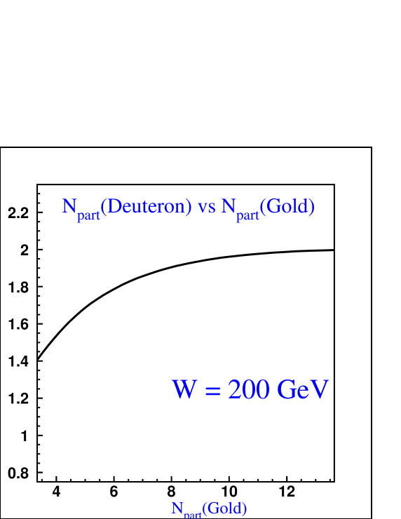
Figure 1: Dependence of the number of participants from the deuteron $N_{part}(Deuteron)$ on the number of participants in the $Au$ nucleus $N_{part}(Gold)$ for $W=200$ GeV.

Using the set of Glauber formulae from KLNS ; KN , Woods–Saxon distribution for the $Au$ nucleus tables and the value of $NN$ inelastic cross section of $42$ mb at $\sqrt{s}=200$ GeV, we obtain the total $d-Au$ cross section of $\sigma^{dAu}=2.26\pm 0.1$ bn, where the estimated error represents the uncertainty in the parameters of the wave function. Computing the differential cross section along the lines of KLNS ; KN , we can also evaluate the average number of participants and collisions in a specific centrality cut; the results are given in Table 1.

Table 2 shows the dependence of the number of participants on the impact parameter of the $d-Au$ collision. The correlation between the number of participants from the deuteron and from the $Au$ nucleus is shown in Fig. 1.

Let us now turn to the discussion of the production dynamics. As before KN ; KL ; KLN , we use the following formula for the inclusive production GLR ; GM :

$$E{d\sigma\over d^{3}p}={4\pi N_{c}\over N_{c}^{2}-1}\ {1\over p_{t}^{2}}\ \times\,\int^{p_{t}}\,dk_{t}^{2}\,\alpha_{s}\ \varphi_{D}(x_{1},k_{t}^{2})\ \varphi_{A}(x_{2},(p-k)_{t}^{2}),$$ (2)

where $x_{1,2}=(p_{t}/\sqrt{s})\exp(\pm y)$ and $\varphi_{A,D}(x,k_{t}^{2})$ is the unintegrated gluon distribution of a nucleus or a deuteron. This distribution is related to the gluon density by

$$xG(x,Q^{2})\,\,=\,\,\int^{Q^{2}}\,\,d\,k^{2}_{t}\,\varphi(x,k_{t}^{2}).$$ (3)

We can compute the multiplicity distribution by integrating Eq. (2) over $p_{t}$, namely,

$$\frac{dN}{dy}\,\,=\,\,\frac{1}{S}\,\int\,\,d^{2}p_{t}E{d\sigma\over d^{3}p};$$ (4)

$S$ is either the inelastic cross section for the minimum bias multiplicity, or a fraction of it corresponding to a specific centrality cut.

Table 2. The numbers of participating nucleons from the deuteron $N_{part}^{D}$, the $Au$ nucleus $N_{part}^{Au}$, and the total number of collisions $N_{coll}$ at different impact parameters $b,{\rm fm}$ for $d-Au$ collisions at $\sqrt{s}=200$ GeV; the densities of participating nucleons from the deuteron ($\rho^{D}_{part},{\rm fm^{-2}}$) and $Au$ ($\rho^{Au}_{part},{\rm fm^{-2}}$) are also shown.

$b,{\rm fm}$	$N_{part}^{D}$	$N_{part}^{Au}$	$N_{coll}$	$\rho_{part}^{D},{\rm fm^{-2}}$	$\rho_{part}^{Au},{\rm fm^{-2}}$
0	1.996	13.645	17.497	0.179	1.091
1	1.996	13.444	17.246	0.180	1.079
2	1.993	12.820	16.465	0.181	1.040
3	1.984	11.702	15.068	0.183	0.972
4	1.960	9.973	12.891	0.186	0.862
5	1.884	7.540	9.761	0.187	0.685
6	1.642	4.670	5.947	0.173	0.435
7	1.097	2.222	2.688	0.115	0.191
8	0.497	0.830	0.940	0.043	0.056
9	0.170	0.270	0.291	0.010	0.013
10	0.052	0.084	0.088	0.002	0.003

Let us assume that the energy is large enough; in this case we can define two saturation scales: one for the deuteron ($Q_{s}(D;x_{1})$) and one for the nucleus ($Q_{s}(A;x_{2})$). It is convenient to introduce two auxiliary variables, namely

$$Q_{s,min}(x)\,\, = \,\,min\left(Q_{s}(D;x),Q_{s}(A;x)\right)\,\,;$$

$$Q_{s,max}(x)\,\, = \,\,max\left(Q_{s}(D;x),Q_{s}(A;x)\right)\,\,.$$ (5)

Of course, in the wide region of rapidities $Q_{s,max}$ is equal to $Q_{s}(A;x)$ while $Q_{s,min}\,\,=\,\,Q_{s}(D;x)$. However, at rapidities close to the nucleus fragmentation region $Q_{s,max}\,\rightarrow Q_{s}(D;x)$ and $Q_{s,min}\,\,\rightarrow\,\,Q_{s}(A;x)$. To see this, let us first fix our reference frame as the center of mass for d-A interaction, with positive rapidities corresponding to the deuteron fragmentation region. As has been discussed before KL ; KLN ; KLM , the HERA data correspond to the power–like dependence of the saturation scale on $x$ GW , namely,

$$Q^{2}_{s}(x)\,\,=\,\,\,Q^{2}_{0}\,\left(\,\frac{x_{0}}{x}\,\right)^{\lambda}$$ (6)

with $\lambda\,\,=\,\,0.288$ GW . Substituting $x_{1}\,\,=\,\,(Q_{s}/W)\,e^{-y}$ and $x_{2}\,\,=\,\,(Q_{s}/W)\,e^{y}$, where $W$ is the energy of interaction, one can see that $Q_{s,min}\,\,=\,\,Q_{s}(A;x)$ for all negative rapidities smaller than $y=y_{c}$; $y_{c}$ is defined as the solution to the equation

$$Q^{2}_{s}(A;x)\,=\,Q^{2}_{0}(A)\left(\,\frac{Q_{0}(A)}{W}\,\right)^{\lambda}\,e^{\lambda\,y_{c}}\,\,=\,\,Q^{2}_{s}(D;x)\,=\,Q^{2}_{0}(D)\left(\,\frac{Q_{0}(D)}{W}\,\right)^{\lambda}\,e^{-\lambda\,y_{c}}$$ (7)

Since $Q^{2}_{0}(A)/Q^{2}_{0}(D)\,\,\propto\,A^{1/3}$ one can see that $y_{c}\,\,\approx\,\,-3.5\div\,-4$ for deuteron - gold collision.

It is convenient to separate three different regions in $p_{t}$ integration in Eq. (4):

1. $p_{t}\,\,<\,\,Q_{s,min}$

   In this region both parton densities for the deuteron and for the nucleus are in the saturation region. This region of integration gives, for $y>y_{c}$,

   $$\frac{dN}{dy}\,\,\propto\,\,\frac{1}{\alpha_{S}}\,S\,Q^{2}_{s,min}\,\,\propto\frac{1}{\alpha_{S}}\,\,N_{part}(Deuteron)$$ (8)

   where we have used the fact that the number of participants is proportional to $SQ_{s}^{2}$, where $S$ is the area corresponding to a specific centrality cut.

2. $Q_{s,max}\,\,>\,\,p_{t}\,\,>\,\,Q_{s,min}$

   For these values of $p_{t}$ we have saturation regime for the nucleus for all rapidities larger than $y_{c}$ (see Eq. (7)) while the deuteron is in the normal DGLAP evolution region. Neglecting anomalous dimension of the gluon density below $Q_{s,max}$, we have $\varphi_{D}(x_{1},k_{t}^{2})\,\,\propto\,\,\frac{1}{\alpha_{S}}\,\,S\,\,Q_{s,min}/k^{2}_{t}$ which leads to, for $y>y_{c}$,

   $$\frac{dN}{dy}\,\,\propto\,\,\frac{1}{\alpha_{S}}\,S\,Q^{2}_{s,min}\,\ln\frac{Q^{2}_{s,max}}{Q^{2}_{s,min}}\,\,\propto\frac{1}{\alpha_{S}}\,\,N_{part}(Deuteron)\,\,\ln\frac{Q^{2}_{s,max}}{Q^{2}_{s,min}}$$ (9)

   This region of integration will give the largest contribution.

3. $\,p_{t}\,\,>\,\,Q_{s,max}$

   In this region both the deuteron and the nucleus parton densities are in DGLAP evolution region.

4. It should be stressed that for $y<y_{c}$ $Q_{S,min}(x)\,=\,Q_{s}(A,x)$ and for all three regions we will get the answer proportional to $S\,Q_{s}^{2}(A,x)\,\propto\,N_{part}(A)$.

The main contribution to Eq. (2) is given by two regions of integration over $k_{t}$: $k_{t}\,\ll\,p_{t}$ and $|\vec{p}_{t}\,-\,\vec{k}_{t}|\,\ll\,p_{t}$. Therefore, we can rewrite Eq. (2) as

$${dN\over dy} = {1\over S}\ \ \int dp_{t}^{2}\left(E{d\sigma\over d^{3}p}\right)=$$ (10)

$$= {4\pi N_{c}\alpha_{S}\over N_{c}^{2}-1}\ \int{dp_{t}^{2}\over p_{t}^{2}}\ \left(\,\varphi_{D}(x_{1},p_{t}^{2})\,\,\int^{p_{t}}\,dk_{t}^{2}\ \varphi_{A}(x_{2},k_{t}^{2})\,\,+\,\,\varphi_{A}(x_{2},p_{t}^{2})\,\,\int^{p_{t}}\,dk_{t}^{2}\ \varphi_{D}(x_{1},k_{t}^{2})\,\right)\,\,=$$

$$= {4\pi N_{c}\alpha_{S}\over N_{c}^{2}-1}\ \,\int^{\infty}_{0}\,\,\frac{d\,p^{2}_{t}}{p^{4}_{t}}\,\,x_{2}G_{A}(x_{2},p^{2}_{t})\,\,x_{1}G_{D}(x_{1},p^{2}_{t})\,\,;$$

where we integrated by parts and used Eq. (3) to obtain the last line in Eq. (10). We use a simplified assumption about the form of $xG$; namely we assume as in Ref. KL that

$$xG(x;p^{2}_{t})\,\,=\,\,\left\{\begin{array}[]{l}\,\,\,\,{\kappa\over\alpha_{S}(Q^{2}_{s})}\,S\,p^{2}_{t}\,\,(1\,-\,x)^{4}\,\,\,\,p_{t}\,<\,Q_{s}(x)\,\,;\\ \\ \,\,\,\,{\kappa\over\alpha_{S}(Q^{2}_{s})}\,S\,Q^{2}_{s}(x)\,\,(1\,-\,x)^{4}\,\,\,\,p_{t}\,>\,Q_{s}(x)\,\,;\end{array}\right.$$ (14)

where the numerical coefficient $\kappa$ can be determined from RHIC data on heavy ion collisions. Since we are interested in total multiplicities which are dominated by small transverse momenta, in Eq. (14) we neglect the anomalous dimension of the gluon densities. The assumption (14) reflects two basic features of the gluon distribution in the saturation region MV1 : the gluon density is large and it varies slowly with transverse momentum. We introduce the factor $(1\,-\,x)^{4}$ to describe the fact that the gluon density is small at $x\,\rightarrow\,1$ as described by the quark counting rules. Substituting Eq. (14) to Eq. (10) we obtain the following formula

$$\frac{dN}{dy}\,\,=\,\,Const\,S\,\,Q^{2}_{s,min}(W,y)\,\,\frac{1}{\alpha_{S}(Q^{2}_{min}(W,y))}\,\times$$ (15)

$$\left[\left(1-\frac{Q_{s,min}(W,y)}{W}\,e^{y}\right)^{4}\,\,+\,\,\{\,\ln(Q^{2}_{max}(W,y)/Q^{2}_{s,min}(W,y))\,\,+\,\,1\,\}\,\left(1-\frac{Q_{s,max}(W,y)}{W}\,e^{y}\right)^{4}\,\right].$$

Eq.(15) is the main result of our paper.

We use Eq. (6) for $W$ and $y$ dependence of the saturation scales, namely

$$Q^{2}_{s}(A;W,y)\,\, = \,\,Q^{2}_{0}(A)\,\left(\,\frac{Q_{0}(A)}{W}\,\right)^{\lambda}\,\,e^{\lambda\,y}\,\,;$$ (16)

$$Q^{2}_{s}(p;W,y)\,\, = \,\,Q^{2}_{0}(p)\,\left(\,\frac{Q_{0}(p)}{W}\,\right)^{\lambda}\,\,e^{\,-\,\lambda\,y}\,\,;$$ (17)

where $y$ is defined in the c.m.s., with deuteron at positive $y$. We assume that the saturation scale for the deuteron is the same as for proton; the constant in Eq. (15) includes $\kappa^{2}$ from Eq. (14) and an additional numerical factor which is the multiplicity of hadrons in a jet with transverse momentum $Q_{s}$. As has been discussed before KN ; KL ; KLN ; KLM  , $S\,Q^{2}_{s}(A)\,\propto\,N_{part}(A)$ and the coefficient in this relation is absorbed in the constant in Eq. (15) as well.

One can see two qualitative properties of Eq. (15). For $y\,>\,0$ and close to the fragmentation of the deuteron, $Q_{s,min}=Q(D)$ and the multiplicity is proportional to $N_{part}(Deuteron)$, while in the nucleus fragmentation region ( $y\,<\,0$ ) $Q_{s,min}=Q(A)$ and $dN/dy\,\propto\,N_{part}(A)$. We thus recover some of the features of the phenomenological “wounded nucleon” model WNM .

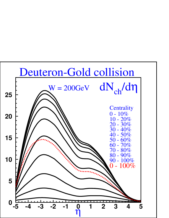
Figure 2: Rapidity dependence $dN/d\eta$ of charged hadron multiplicities in deuteron - gold collision for different centrality cuts; also shown is the minimum bias distribution ($0-100\%$).

In Fig. 2 we plot our prediction for the dependence of multiplicity on rapidity and centrality at $W\,=\,200$ GeV. The transformation from rapidity to pseudo–rapidity was done as described in Ref.KL ; this transformation is responsible for the structure in the shape of the distributions around zero pseudo–rapidity. We also show the minimum bias distribution obtained by explicit integration over centralities.

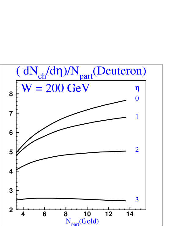
Figure 3: $N_{part}$ dependence for positive ($d$ fragmentation region) rapidities for deuteron-gold interactions at $W=200$ GeV.

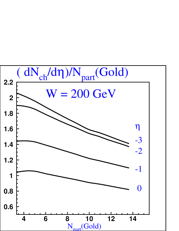
Figure 4: $N_{part}^{Au}$ dependence for negative ($Au$ fragmentation region) rapidities for deuteron-gold interactions at $W=200$ GeV.

One can see that the dependence on centrality cut is not so dramatic as for $Au-Au$ collisions (see KN ; KL ; KLN ). The reason for this is the fact that the yields depend mostly on the number of participants in the deuteron which does not change very fast with centrality – see Fig. 1. The $N_{part}$ dependence of the multiplicity is shown in Fig. 3 and Fig. 4 in a different way, analogous to nucleus–nucleus collisions. For positive rapidities, we plot the multiplicity per $N_{part}(deuteron)$, while for negative values of rapidity ( nucleus fragmentation region) it is natural to divide by $N_{part}(A)$. The result at mid–rapidity $\eta=0$ is shown in both figures; the apparently different behavior follows from the dependence of the $N_{part}(Deuteron)$ as a function of $N_{part}(Gold)$, which is shown in Fig. 1.

For the $Au$ nucleus, we determine the saturation scale similarly to KN ; KL ; for the proton, we use $Q^{2}_{0}(proton)\,\simeq\,0.3\,\ GeV^{2}$. This value follows from the value of $Q^{2}_{s}(Gold)$ if we use $Q^{2}_{0}(proton)\,=\,(N_{part}(D)/N_{part}(Gold))\,\times\,Q^{2}_{s}(Gold)$. Whether or not it makes sense to describe the proton wave function as saturated at $Q_{0}\simeq 0.5$ GeV is a difficult question, which represents the main uncertainty in our calculations. We address this question by applying our approach to hadron multiplicities in the $NN$ interaction at collider energies; the results of our calculations are shown in Fig. 5. The formulae which we used to obtain Fig. 5 are our Eq. (15) where we use $Q_{s}(A;x)=Q_{s}(p,x)$ and Eq. (16) with $Q_{0}(A)=Q_{0}(p)$; the absolute normalization will be discussed below.

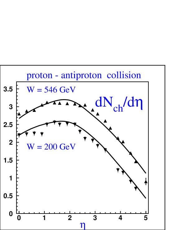
Figure 5: Rapidity dependence for $dN/d\eta$ for proton - antiproton collision at $W=200$ and $546$ GeV. The solid lines correspond to Eq. (15) with both saturation scales set equal to the proton one. The data is taken from PDG .

Now let us discuss the normalization of our results – the value of the factor $Const$ in Eq. (15). This factor includes the normalization of the gluon density inside the saturation region ( $\kappa$ in Eq. (14) ), the gluon liberation coefficient $c$ (see Ref. AHM ), which says what fraction of gluons in the initial partonic wave function can be produced, the factor $n_{jet}$ – the multiplicity of hadron in a partonic jet with the typical momentum $Q_{s}$, and the coefficient $\xi$ in the relation $N_{part}=\xi\,S\,Q^{2}_{s}$. For most of these factors we have only estimates. The value of $c$ was recently computed numerically on the lattice RAJU , with the result $c\approx 0.5$. $n_{jet}$ can be taken from $e^{+}e^{-}$ annihilation into jets. The value of $\kappa$ can be calculated deeply in the saturation region MV1 . However, if we use the RHIC data on $Au-Au$ collisions, to determine $Const$ we need to know only the value of $c$. Indeed, using the formulae for nucleus–nucleus multiplicities from Ref. KL we can calculate

$$\frac{dN_{hadron}(A-A)}{d\eta}(\eta=0)\,\,=\,\,Const(A-A)\ \,(N_{part}/2)\,\,2\,\,\ln(Q^{2}_{s}(W=130\,GeV)/\Lambda_{QCD}^{2}).$$ (18)

Using $N_{part}\approx\,339$ KN for 6% centrality cut, we extract the value of $Const(A-A)$ in Eq. (18) by using the experimental number for $dN_{hadron}(A-A)/d\eta=555\pm 12(stat)\pm 35(syst)$ :

$$Const(A-A)\,\,=\,\,0.56\,\,.$$ (19)

The value of $Const$ in Eq. (15) is then equal to

$$Const\,\,=\,\,\frac{Const(A-A)}{c}$$ (20)

if we assume that in proton - nucleus collisions all gluons from the initial wave function of the proton are liberated.

However, the normalization constant that we used to fit the proton - antiproton data in Fig. 5 turns out to be different, by factor of $\simeq 0.67$, from what would be given by Eq. (20) with $c=0.5$. We think that the main reason for this is the use of Eq. (4) for the multiplicity, where we divide by the interaction cross section. For ion–ion and hadron–ion collisions the geometrical picture for the cross section works quite well, so the inelastic cross section in Eq. (4) can be replaced by the interaction area; however, this is not the case for hadron - hadron scattering. In describing the data (see Fig. 5), we have used the formula Eq. (4) with $S\,\rightarrow\,\sigma_{inel}(p-\bar{p})$. If we extract the effective proton radius from the slope $b\simeq 10\ GeV^{-2}$ of elastic cross section $d\sigma_{el}/dt\sim\exp(-bt)$ (where $t$ is the invariant momentum transfer) at the energies of interest we get, assuming Gaussian profile function, $R^{eff}_{P}\simeq 0.9$ fm (which is also close to the proton electromagnetic radius). Using this value for $R^{eff}_{P}$ and $\sigma_{inel}=42$ mb for $W=200$ GeV, we see that the geometrical cross section $S$ differs from $\sigma_{inel}$ by factor of $S/\sigma_{inel}\,\approx\,0.6$, which is close to explaining the discrepancy between $pp$ and $AA$ data that we have. To check this hypothesis, we calculated $dN/d\eta$ for a higher energy of $W\,=\,546$ GeV. The energy dependence comes from the energy dependence of the saturation scale ( see Eq. (6)) and of the factor $S/\sigma_{inel}$, in which we use the experimental values of $\sigma_{inel}$. In Fig. 5 one can see that the data at higher energies is reproduced. Nevertheless, the description of the proton structure represents the main uncertainty in our calculations.

To summarize, we derived the formulae for the rapidity and centrality dependencies of hadron production in $dA$ collisions at collider energies, and used them to predict what will happen in the forthcoming $dAu$ run at RHIC. The results appear very sensitive to the production dynamics; we thus expect that the $dA$ data will significantly improve the understanding of multi–particle production in the high parton density regime.

We thank E. Gotsman, P. Jacobs, J. Jalilian-Marian, U. Maor, L. McLerran, D. Morrison, R. Venugopalan and W. Zajc for useful discussions.

E.L. thanks the DESY Theory Division for the hospitality. The work of D.K. is supported by the U.S. Department of Energy under Contract DE-AC02-98CH10886. This research was supported in part by the BSF grant # 9800276, and by the GIF grant # I-620-22.14/1999, and by the Israel Science Foundation, founded by the Israeli Academy of Science and Humanities.

I Erratum added on March 8, 2004

After the publication of our paper, the experimental data on hadron multiplicities in $dAu$ collisions at RHIC have been presented phobos-e ; brahms-e ; star-e . While the predicted multiplicity distributions are consistent with the data within $\simeq 30\%$, a detailed comparison exhibits discrepancies both in the shape of rapidity distributions and in centrality dependence.

Should we consider this discrepancy as an argument against the Color Glass Condensate approach, or does it stem from something that we overlooked in our calculations? Our analysis presented below shows that the disagreement with the data originates mainly in the centrality determination procedure. In our paper, as well as in the previous publications dedicated to $Au-Au$ collisions, we used the optical Glauber model to evaluate the numbers of participants $N_{part}$ and collisions $N_{coll}$ corresponding to a particular centrality cut imposed on the multiplicity distribution. Meanwhile, the experiments use Monte Carlo realizations of the Glauber model, which also take into account the geometry and acceptance of the detector.

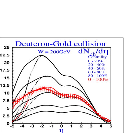
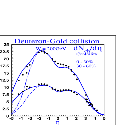
Fig. 6 a)	Fig. 6 b)

Figure 6: Charged multiplicity distribution in pseudo-rapidity for different centrality cuts in $d-Au$ collisions. Fig. 1 a) shows the comparison of our predictions to the PHOBOS minimum-bias data phobos-e , and Fig. 1 b) – to the data from BRAHMS brahms-e .

Already for the $Au-Au$ system it has been noted that in peripheral collisions, when $N_{part}$ and $N_{coll}$ become small, the discrepancy between the optical and Monte Carlo realizations becomes significant. Nevertheless, for $N_{part}\geq 70$ the agreement between the two approaches was reasonable, on the order of $\sim 10\%$. However in $d-Au$ collisions, where the numbers of participants and collisions are always relatively small, the differences in centrality determination strongly affect the comparison of our predictions to the data at all centralities: indeed, the discrepancies between the number of participants given in our Table 1 and presented by the experimental Collaborations phobos-e ; brahms-e ; star-e sometimes are as big as $\sim 50\%$. Part of the problem stems from the fact that in the optical approach in peripheral collisions $N_{part}$ can be smaller than two – this is because the overlap integral in this case has a meaning of the probability to have $N_{part}=2$; in the Monte Carlo approach, one instead triggers on the inelastic interaction event, so the number of participants is always $N_{part}\geq 2$. Note that since the shape of our rapidity distributions (see Eq.(12)) depends on the number and density of participants in $Au$ and deuterium separately, it is also affected by the uncertainty in centrality determination.

To investigate the influence of these differences in centrality determination, we have repeated the calculations according to our Eq.(12), but using experimental numbers of $N_{part}$ and $N_{coll}$. This can be done by multiplying our $\rho^{D}_{part}$ and $\rho^{A}_{part}$ by the factor $\frac{N^{exp}_{part}}{N^{exp,MB}_{part}}\,\cdot\frac{N^{our,MB}_{part}}{N^{our}_{part}}$. We found that this alone removes almost all of the discrepancy with the data. Moreover, as we discussed in the paper, our master equation Eq.(12) is based on the assumption that the gluon distribution inside the proton can be effectively described as a saturated one. As we emphasized, the value of the effective proton saturation momentum is somewhat uncertain, and we used $Q_{s}^{2}(p;W=200\,{\rm GeV};y)\,=\,0.25\,{\rm GeV}^{2}$. We find that a larger value $Q_{s}^{2}(p;W=200\,{\rm GeV};y)\,=\,0.34\,{\rm GeV}^{2}$ improves the fit. The results are shown in Fig.1 by the dashed lines. One can see that the agreement is now quite good, with an exception of the gold fragmentation region. The Color Glass Condensate approach cannot be justified in this region where the nuclear distribution is probed at large Bjorken $x$; the fragmentation of the $Au$ participants is expected to dominate there. If we assume that $dN/dy$ is equal to $N^{Au}_{part}\times dN(pp)/dy$ in the region of $-5<y<-3$, we get the results shown by the solid curves in Fig.1.

References

-
(1)
I. G. Bearden [BRAHMS Collaboration], nucl-ex/0207006;
nucl-ex/0112001; Phys. Lett. B 523, 227 (2001),
nucl-ex/0108016; Phys. Rev. Lett. 87 (2001) 112305;
nucl-ex/0102011; nucl-ex/0108016;
J.J. Gaardhoje et al., [ BRAHMS Collaboration ], Talk presented at the “Quark Gluon Plasma” Conference, Paris, September 2001. -
(2)
A. Bazilevsky [PHENIX Collaboration],
nucl-ex/0209025;
A. Milov [PHENIX Collaboration], Nucl. Phys. A 698, 171 (2002), nucl-ex/0107006;
K. Adcox et al. [PHENIX Collaboration], Phys. Rev. Lett. 87, 052301 (2001), nucl-ex/0104015; Phys. Rev. Lett. 86, 3500 (2001), nucl-ex/0012008. -
(3)
B. B. Back et al. [PHOBOS Collaboration],
Phys. Rev. Lett. 85, 3100 (2000),
hep-ex/0007036; Phys. Rev. C 65, 061901 (2002),
nucl-ex/0201005; nucl-ex/0108009;
Phys. Rev. Lett. 87, 102303 (2001),
nucl-ex/0106006; Phys. Rev. Lett. 85, 3100 (2000),
hep-ex/0007036;
M. D. Baker [PHOBOS Collaboration], nucl-ex/0212009. -
(4)
Z. b. Xu [STAR Collaboration],
nucl-ex/0207019;
C. Adler et al. [STAR Collaboration], Phys. Rev. Lett. 87, 112303 (2001), nucl-ex/0106004. - (5) D. Kharzeev and M. Nardi, Phys. Lett. B 507 (2001) 121.
- (6) D. Kharzeev and E. Levin, Phys. Lett. B 523 (2001) 79.
- (7) D. Kharzeev, E. Levin and M. Nardi, “The onset of classical QCD dynamics in relativistic heavy ion collisions,” hep-ph/0111315.
- (8) L. V. Gribov, E. M. Levin and M. G. Ryskin, Phys. Rep. 100 (1983) 1.
-
(9)
A.H. Mueller and J. Qiu, Nucl.Phys. B 268 (1986) 427;
J.-P. Blaizot and A.H. Mueller, Nucl. Phys. B 289 (1987) 847. - (10) L. McLerran and R. Venugopalan, Phys. Rev. D 49 (1994) 2233; 3352; D 50 (1994) 2225.
- (11) Yu.V. Kovchegov, Phys. Rev. D 54 (1996) 5463; J. Jalilian-Marian, A. Kovner, L. McLerran, H. Weigert, Phys.Rev. D55 (1997) 5414; E. Iancu and L. McLerran, Phys.Lett. B510 (2001) 145; A. Krasnitz and R. Venugopalan, Phys. Rev. Lett.84 (2000) 4309; E. Levin and K. Tuchin, Nucl. Phys. B573 (2000) 833; A693 (2001) 787; A691 (2001) 779; A.H. Mueller,“Parton saturation: An overview,” hep-ph/0111244; E. Iancu, A. Leonidov and L. D. McLerran, Nucl. Phys. A692 (2001) 583, hep-ph/0011241; E. Iancu, K. Itakura and L. McLerran, Nucl. Phys. A708 (2002) 327, hep-ph/0203137.
-
(12)
L. McLerran and J. Schaffner-Bielich, Phys. Lett. B514 (2001) 29;
J. Schaffner-Bielich, D. Kharzeev, L. D. McLerran and R. Venugopalan, Nucl. Phys. A 705 (2002) 494. -
(13)
S. Mioduszewski [PHENIX Collaboration], nucl-ex/0210021;
T. Sakaguchi [PHENIX Collaboration], nucl-ex/0209030;
D. d’Enterria [PHENIX Collaboration],nucl-ex/0209051;
K. Adcox et al. [PHENIX Collaboration], nucl-ex/0207009, Phys. Rev. Lett. 88, 022301 (2002),nucl-ex/0207003;
C. Adler et al. [STAR Collaboration], Phys. Rev. Lett. 89 (2002) 202301, nucl-ex/0206006;
J. C. Dunlop [STAR Collaboration], Nucl. Phys. A698, 515 (2002);
M. Baker et al. [PHOBOS Collaboration], in Phobos . - (14) D. Kharzeev, E. Levin and L. McLerran, “Parton saturation and scaling of semi-hard processes in QCD”, hep-ph/0210332.
- (15) A.H. Mueller, Nucl. Phys. B572 (2000) 227.
- (16) A. Krasnitz, Y. Nara and R. Venugopalan, “Gluon production in the color glass condensate model of collisions of ultrarelativistic finite nuclei,” hep-ph/0209269, Nucl. Phys. AA702 (2002) 227;Phys. Rev. Lett. 87 (2001) 192302 hep-ph/0108092 and references therein.
- (17) K. Golec-Biernat and M. Wüsthof, Phys. Rev. D59 (1999) 014017; Phys. Rev. D60 (1999) 114023; A. Stasto, K. Golec-Biernat and J. Kwiecinski, Phys. Rev. Lett. 86 (2001) 596.
- (18) E. M. Levin and M. G. Ryskin, Phys. Rept. 189 (1990) 267.
- (19) E. M. Levin and M. G. Ryskin, Nucl. Phys. B304 (1988) 805.
- (20) A. Dumitru and L.D. McLerran, Nucl. Phys. A700 (2002) 492.
- (21) F. Gelis and J. Jalilian-Marian, Phys. Rev. D66 (2002) 014021.
- (22) J. T. Lenaghan and K. Tuominen, “Saturation and pion production in proton nucleus collisions,” hep-ph/0208007.
- (23) A. Dumitru and J. Jalilian-Marian, Phys. Rev. Lett. 89 (2002) 022301; Phys. Lett. B547 (2002) 15.
- (24) L. Hulthen and M. Sugawara, “Handbuch der Physik”, vol.39 (1957).
- (25) D. Kharzeev, C. Lourenço, M. Nardi and H. Satz, Z.Phys.C74(1997) 307.
- (26) C.W. De Jager, H. De Vries and C. De Vries, Atom. Nucl. Data Tabl. 14 (1974) 479.
- (27) E. Laenen and E. Levin, Ann. Rev. Nuc. Part. Sci. 44 (1994) 199; Yu. V. Kovchegov and D. Rischke, Phys. Rev. C56 (1997) 1084; M. Gyulassy and L. McLerran, Phys. Rev. C56 (1997) 2219; Yu. V. Kovchegov and A. H. Mueller, Nucl. Phys. B529 (1998) 451 M. A. Braun, Eur. Phys. J. C16 (2000) 337, hep-ph/0010041, hep-ph/0101070; Yu. V. Kovchegov, Phys. Rev. D64 (2000) 114016; Yu. V. Kovchegov and K. Tuchin, Phys. Rev. D65 (2002) 074026 hep-ph/0111362.
- (28) A. Bialas, M. Bleszynski and W. Czyz, Nucl.Phys. B111 (1976) 461.
- (29) Particle Data Group, Eur. Phys. J. 15 (2000) 1.
- (30) B.B. Back et al [PHOBOS Collaboration], nucl-ex/0311009; R. Noucier [PHOBOS Collaboration], Talk at Quark Matter 2004 Conference, Oakland, California, January 2004.
- (31) I. Arsene et al [BRAHMS Collaboration], nucl-ex/0401025.
- (32) J. Putschke et al [STAR Collaboration], poster presented at Quark Matter 2004 Conference, Oakland, California, January 2004.