hep-ph/0212305
Cosmological Baryon Asymmetry and Neutrinos:
Baryogenesis via Leptogenesis in Supersymmetric Theories
Koichi Hamaguchi
Deutsches Elektronen-Synchrotron DESY, D-22603, Hamburg, Germany
Dr.thesis submitted to
Department of Physics, University of Tokyo
January 2002
Ph.D thesis
Cosmological Baryon Asymmetry and Neutrinos:
Baryogenesis via Leptogenesis in Supersymmetric Theories
Koichi Hamaguchi
Department of Physics, University of Tokyo, Tokyo 113-0033, Japan
Submitted to Department of Physics, University of Tokyo: January 2002
Accepted: February 2002
Revised to submit to the eprint arXiv: December 2002
Chapter 1 Introduction
1.1 Overview
The origin of baryon asymmetry (matter-antimatter asymmetry) in the present universe is one of the fundamental puzzles in particle physics as well as in cosmology. Assuming an inflationary phase in the early universe, any initial baryon asymmetry is diluted and becomes essentially zero during the inflation. Therefore, the observed baryon asymmetry should be generated dynamically after the inflation. Such a dynamical generation of baryon asymmetry (baryogenesis) is possible if the following three conditions are satisfied; (i) baryon-number violation, (ii) - and -violations, and (iii) departure from thermal equilibrium, which are known as the Sakharov’s three conditions [1].
The original idea of the baryogenesis in the grand unified theory (GUT) [2] satisfies all of these conditions [3], and provides an elegant interplay between particle physics and cosmology. Actually, the GUT [4] unifies baryons and leptons in the same gauge multiplets and predicts the existence of baryon number violation, the delayed decay of superheavy GUT particle satisfies the out-of-equilibrium condition, and its -violating asymmetric decay into baryons and antibaryons can offer a net baryon asymmetry.
On the other hand, the electroweak gauge theory itself violates the baryon asymmetry by a quantum anomaly [5]. This effect is highly suppressed by a large exponential factor at zero temperature, and hence the stability of the proton is practically guaranteed. However, it was found that in the early universe at high temperatures above the electroweak scale, the baryon-number violating interaction is not suppressed and even be rapid enough to be in thermal equilibrium [6]. An important point here is that this baryon number violating (“sphaleron”) process violates lepton () number as well as baryon () number, and it conserves a linear combination of them, . Therefore, if the baryon asymmetry is produced in -conserving processes, like those in the GUT, it would be washed out by the sphaleron effect before the electroweak phase transition, and hence no baryon asymmetry can remain until the stage of big-bang nucleosynthesis to generate the light nuclei.
The existence of the sphaleron effect opens a new possibility of baryogenesis, the generation of baryon asymmetry at electroweak phase transition [6, 7]. This mechanism does not use any -violation, and the baryon asymmetry is generated by the sphaleron-induced -violating process. (Hence, same amount of baryons and leptons are produced.) As other baryogenesis scenarios have, this mechanism also has a double-edged behavior, i.e., the produced baryon (and lepton) asymmetry tends to be washed out afterwards by the sphaleron process itself. In order to avoid the erasure of the produced baryon asymmetry, the electroweak phase transition must be strongly first-order. However, in the case of the minimal standard model with one Higgs doublet, it turns out that, for Higgs masses allowed by current experimental bounds, the electroweak transition is too weakly first order or just a smooth transition, which excludes the electroweak baryogenesis in the standard model. Although the extension of the standard model to the supersymmetric version may cure this difficulty, there remains only a small parameter range [8].
Therefore, it seems natural to consider that the baryon asymmetry was generated before the electroweak phase transition. As long as we consider a baryogenesis above the electroweak scale, some -violating interaction is mandatory, since the sphaleron process washes out any baryon asymmetry in the universe unless there exists nonzero asymmetry. (Namely, the first one of the Sakharov’s conditions, (i) -violation, should be replaced with (i)’ -violation.) This means, on the other hand, as first suggested by Fukugita and Yanagida [9], that the lepton-number violation is enough for baryogenesis and explicit baryon-number violation is not necessarily required. Actually, there now exists an implication of lepton-number () violation, whereas there has been discovered no evidence for baryon-number () violations: that is, the neutrino oscillation.
Neutrino oscillation [10, 11],111Very recently the KamLAND experiment has announced the first results, which exclude all oscillation solutions but the ’Large Mixing Angle’ solution to the solar neutrino problem [12]. especially the strong evidence for the atmospheric neutrino oscillation reported in 1998 by the Super-Kamiokande Collaboration [10], is one of the greatest discoveries in particle physics after the success of the standard model. The experimental data strongly suggest that the neutrinos have small but finite masses, impelling the standard model of particle physics to be modified.
Such tiny masses of light neutrinos are naturally understood if we introduce heavy right-handed Majorana neutrinos to the standard model, in terms of so-called seesaw mechanism [13]. Because the right-handed neutrinos are singlets under the standard gauge symmetries, they can have Majorana masses as well as Yukawa couplings to the left-handed leptons () and Higgs () doublets:222Here, we have omitted the family- and -indices for simplicity.
| (1.1) |
where we have taken the to be the Majorana mass eigenstates. Then by integrating out the heavy right-handed neutrinos, we obtain the small Majorana masses for light neutrinos, .
A crucial observation in the lagrangian Eq. (1.1) is that the Majorana mass term represents nothing but a lepton number () violation, actually a -violation. In fact, the heavy right-handed neutrinos have two distinct decay channels into leptons and anti-leptons, and produce asymmetry if the Yukawa couplings violate the and if the decay is out of thermal equilibrium. The produced lepton asymmetry is partially converted into baryon asymmetry via the aforementioned sphaleron effect, which explains the baryon asymmetry in the present universe. This is the original idea of the leptogenesis [9].
We should also note that if we assume a gauged symmetry, the existence of three generations of the right-handed neutrinos are automatically required in order to cancel the gauge anomaly. As well known, the symmetry is the unique extra symmetry which can be gauged consistently with the standard model. Furthermore, the breaking of this symmetry naturally provides large Majorana masses to the right-handed neutrinos, which leads to the tiny neutrino masses via the seesaw mechanism. It should be noticed that the symmetry is consistent with the GUT, and is embedded in larger GUT groups such as .
Meantime, the supersymmetry (SUSY) [14] has been attracting wide interests in particle physics as one of the best candidates for new physics beyond the standard model. It protects the huge hierarchy between the electroweak scale and unification (or Planck) scale against the quadratically divergent radiative corrections, and the particle contents of the minimal SUSY standard model (MSSM) lead to a beautiful unification of the three gauge couplings of the standard model at the scale [15], which strongly suggests the SUSY GUT [16]. The MSSM also gives a natural framework to break the electroweak symmetry radiatively [17]. On the other hand, from the viewpoint of cosmology, SUSY provides an ideal dark matter candidate, the lightest SUSY particle [18]. It also protects the flatness of the inflaton potential against the radiative corrections, which is inevitable for successful inflation.
However, SUSY also causes a cosmological difficulty if the reheating temperature of the inflation is too high, that is, the cosmological gravitino problems [19, 20]. After the end of the inflation, the gravitinos are produced by scattering processes of particles from the thermal bath, and its abundance is proportional to the reheating temperature. Because the gravitino’s interaction is suppressed by the gravitational scale, it has a very long lifetime unless it is completely stable, and its decay during or after the big-bang nucleosynthesis (BBN) epoch (– sec) might spoil the success of the BBN [19, 21]. On the other hand, if the gravitino is completely stable, its present mass density must be below the critical density of the present universe [20]. In both cases, the primordial gravitino abundance should be low enough, and hence the reheating temperature of the inflation is severely constrained from above, depending on the gravitino mass.
In this thesis, we study in detail several leptogenesis scenarios in the framework of the SUSY. There have been proposed, in fact, various leptogenesis scenarios depending on the production mechanisms of the right-handed neutrinos:
-
•
In the simplest and the most conventional leptogenesis mechanism, the right-handed neutrino is produced by thermal scatterings [9, 22]. The delayed decay of the right-handed neutrino satisfies the out-of-equilibrium condition à la the original GUT baryogenesis. This mechanism requires a relatively high reheating temperature to produce the heavy right-handed neutrino, and the aforementioned gravitino problem makes it somewhat difficult, depending on the gravitino mass.
-
•
Another mechanism is given when the right-handed neutrinos are produced non-thermally in inflaton decay [23]. In this scenario the reheating temperature can be lower than the case of thermal production, and the gravitino problem is avoided in a wider range of gravitino mass.
-
•
The third mechanism is inherent in the SUSY. The lepton asymmetry is produced by the decay of coherent oscillation of the right-handed “s”neutrino, which is the supersymmetric scalar partner of the right-handed neutrino [24, 25]. If the right-handed sneutrino’s oscillation dominates the energy density of the universe, the gravitino problem is drastically ameliorated [26].
In the framework of SUSY, there is yet another, completely different mechanism. The lepton asymmetry is produced not by the right-handed neutrino decay, but by a coherent oscillation (actually, a rotation) of a flat direction field including the lepton doublet :
- •
1.2 Outline of this thesis
The outline of this thesis is as follows. The rest of this chapter is devoted to some reviews. We briefly mention the observed baryon asymmetry in Sec. 1.3. A review of the sphaleron effect, which is a crucial ingredient of the leptogenesis, is given in Sec. 1.4. We also briefly review the results of the cosmological gravitino problems in Sec. 1.5.
In Chapter 2, we discuss leptogenesis scenarios by the decay of the right-handed (s)neutrino. First, we study the asymmetric decay of the right-handed neutrino into leptons and anti-leptons in Sec. 2.1. The conventional leptogenesis mechanism where the right-handed neutrinos are thermally produced is briefly discussed in Sec. 2.2. Then we perform a comprehensive study of the leptogenesis mechanism in inflaton decay in Sec. 2.3, adopting various SUSY inflation models. In Sec. 2.4, we investigate the leptogenesis from coherent right-handed sneutrino.
In the latter half of this thesis, in Chapter 3, we perform a detailed analysis on the leptogenesis via flat direction. This scenario may require another overview, which will be given in Sec. 3.1. Here we mention one point, that the most important parameter in this scenario which determines the baryon asymmetry is the mass of the lightest neutrino, . (Notice that the data from neutrino-oscillation experiments [10, 11, 12] suggest the difference of the neutrino mass squared, indicating the masses of the heavier neutrinos, and .) It is amazing that the observed baryon asymmetry, which was generated in the very early universe, is directly related to such a low-energy physics, the neutrino mass.
1.3 Baryon asymmetry
We will use the following value for the baryon asymmetry in the present universe [28, 29]:
| (1.2) |
where and are baryon and anti-baryon number density, respectively, and is the entropy density of the universe. This ratio takes a constant value, as long as the baryon number is conserved and no entropy production takes place. Notice that and hence in the present universe. (We sometimes call the just “baryon number density,” for simplicity.) This value is determined from the big-bang nucleosynthesis (BBN). The BBN occurs at the temperature of –, or equivalently at the cosmic time – sec, and generates light nuclei, D, 3He, 4He, and 7Li. (For reviews, see, for example, Refs. [28, 29].) The agreement between the predictions of the BBN theory for the abundances of these light nuclei and the primordial abundances of them (which are inferred from observational data) is one of the most important successes of the standard big-bang cosmology. Actually, the theory of the BBN has basically only one free parameter,333We assume the number of neutrino generations to be three. As well known, this fact itself is one of the most important implications of the BBN. i.e., the baryon asymmetry, and all the above light-element abundances are well explained with in the range of Eq. (1.2).
To demonstrate the smallness of the baryon asymmetry, let us calculate the baryon-number and anti-baryon number density at high temperature. For example, consider a temperature between the QCD phase transition and electroweak phase transition, say, . At this temperature, all the baryons and anti-baryons are expected to exist as quarks and anti-quarks, and they are well in thermal equilibrium. The ratio of the baryon-number and anti-baryon-number densities to the entropy density are then given by
| (1.3) |
where we have used Eq. (B.23). Compared with Eq. (1.2), this means, , i.e., there were (1,000,000,000+1) baryons per 1,000,000,000 anti-baryons at this epoch.
1.4 Sphaleron
In this section, we give a brief review of the “sphaleron” effect, which is a crucial ingredient of the leptogenesis. If the lepton asymmetry is successfully generated, it is partially converted into the baryon asymmetry at equilibrium thanks to the sphaleron-induced baryon and lepton number violating process, which then explains the observed baryon asymmetry in the present universe.
At the classical level, the Lagrangian of the standard gauge theory clearly conserves the baryon () and lepton () numbers. However, as was first pointed out by ’t Hooft [5], both and are violated by quantum effects:
| (1.4) |
where is the number of fermion generations and and are the coupling constant and the field strength of the gauge group, respectively. It was shown later that the gauge theory has a non-contractible loop (path) in the field configuration space, which connects topologically distinct vacua with different baryon and lepton numbers [30], and it was found that the highest energy configuration along this “path” corresponds to a spatially localized and static, but unstable solution [31, 32]. This solution was named “sphaleron”. Since this sphaleron solution is a saddle point of the field potential energy, its energy represents the height of the barrier between the vacua with different baryon and lepton numbers (see Fig. 1.1).

At zero temperature, the rate of baryon (and lepton) number violating process via a tunneling between the topologically distinct vacua (for example, proton decay) is extremely small [5], since it is suppressed by the factor of . However, as suggested by Kuzmin, Rubakov, and Shaposhnikov [6, 33], such processes are not suppressed and can even be efficient at temperatures close to (and above) the electroweak phase transition. The transition of the fermion number occurs simultaneously for each fermion doublets, so that the total changes in the numbers of baryons and leptons are . Therefore, is conserved. (This is clear from the absence of the anomaly in in Eq. (1.4).)
Let us roughly estimate the temperature above which this -violating process becomes in thermal equilibrium, according to Ref. [6]. We assume that the electroweak phase transition is the second order, and consider the temperature , where is the critical temperature above which the vacuum expectation value of the Higgs field vanishes. In such a situation, the transition from one vacuum (say, and ) to the next vacuum ( and ) occurs at the rate [6]
| (1.5) |
where dimensionless factor depends on the ratio and the coupling constants.444See comments below. represents the free energy of the sphaleron configuration (at temperature ), which is given by [31]
| (1.6) |
where depends on the gauge coupling and the 4-point coupling constant of the Higgs potential as , varying from () to () [31]. The rate in Eq. (1.5) should be compared with the Hubble expansion rate . ( is the reduced Planck scale and is defined in Appendix B.2.) Then, it is found that the sphaleron rate in Eq. (1.5) indeed exceeds the Hubble expansion rate for , where is given by
| (1.7) |
Here, we have neglected the and compared with the large number . Recalling that approaches to zero for , this occurs below the critical temperature, i.e., . Therefore, the sphaleron-induced -violating process becomes in equilibrium for . Precisely speaking, a more careful treatment including the prefactor , which turns out to be proportional to [34], is required. A numerical estimation shows that is just below the critical temperature, , for [35].
The evaluation of the “sphaleron” rate for is a complicated problem, since the sphaleron configuration no longer exists in the symmetric phase.555Although the saddle-point sphaleron solution does not exist in the symmetric phase, we will call this anomalous -violating process “sphaleron” also for . Naively thinking, there seems no reason for the -violating processes to be suppressed, since the potential barrier vanishes. Actually, theoretical arguments as well as numerical calculations suggest [36] that the sphaleron rate per unit time per unit volume is for , where . By using their result, it is found that the sphaleron rate exceeds the Hubble expansion rate for .
Therefore, the sphaleron-induced -violating process is in thermal equilibrium in the range of
| (1.8) |
relation between baryon and lepton asymmetry
Let us calculate the relation between the baryon and lepton number in the presence of the sphaleron process, by means of the analysis of the chemical potentials [37, 38]. At first sight, it seems that the relation is just given by since the sphaleron effect violates , preserving . However, as we will see, a nontrivial relation is derived if there exists a non-vanishing asymmetry.
We first consider the standard model without supersymmetric particles, but with Higgs doublets, (), and generations of fermions, i,e., left-handed quark doublets , right-handed up-type and down-type quarks and , left-handed lepton doublets and right-handed charged leptons (). Hereafter, we consider the symmetric phase . Hence, the symmetry recovers. We denote the asymmetry of the number density of particle by , which is related to the chemical potential of that particle as follows [see Eq. (B.24)]:
| (1.12) |
Therefore, the baryon and lepton number asymmetries are given by
| (1.13) | |||||
where we have used the fact that the chemical potentials of particles in the same gauge multiplet are the same, which is ensured by the gauge interactions. (Note that the is also recovered, since we consider .)
In the following, we derive the relations between the chemical potentials . First of all, we assume that all the Higgs doublets have the same chemical potentials due to the mixings between themselves, i.e., . (If there is a Higgs doublet with a conjugate quantum number, like in the MSSM, we redefine the chemical potential of that Higgs doublet with an additional minus sign.) Then, the interactions via Yukawa couplings
| (1.14) |
lead to
| (1.15) |
Here, we have taken a basis of gauge eigenstates for the quarks. Thus, because of the mixing in the Yukawa couplings, the chemical potentials of the quarks become generation independent: , and (). Notice that the relations in Eq. (1.4) hold as long as these interactions are in thermal equilibrium, and even the electron Yukawa coupling, which is the smallest one, is in equilibrium for . Next, the charge neutrality of the universe requires vanishing total charge:
| (1.16) |
where denotes the charge of particle . This leads to
| (1.17) |
Finally, the sphaleron interaction can be understood as
| (1.20) |
which leads to
| (1.21) |
From Eqs. (1.4), (1.17) and (1.21), all the chemical potentials can be written in terms of independent ones, say, . Then, from Eq. (1.4), we obtain
| (1.22) | |||||
Because the conserved quantity is the asymmetry in the present analysis,666Actually, not only the total but each () is conserved in the present situation. it is suitable to rewrite the above relations in terms of :
| (1.23) |
where is given by [37]
| (1.24) |
In the case of the standard model, and yield .
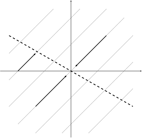
We can see from Eq. (1.23) that, if asymmetry is absent, any baryon asymmetry vanishes at equilibrium in the presence of the sphaleron effect. (See the arrow (i) in Fig. 1.2.) On the other hand, if there occurs a successful leptogenesis, i,e., if nonzero lepton asymmetry (and hence asymmetry) is generated in an out-of-equilibrium way, it is partially converted into baryon asymmetry [9]. (See the arrow (ii) in Fig. 1.2.) The amount of the baryon asymmetry at equilibrium is obtained from Eq. (1.23) as
| (1.25) |
where we have normalized the number densities by the entropy density, so that they become constant against the expansion of the universe.
In the case of the MSSM, we have an additional Higgs doublet as well as supersymmetric partners. Let us calculate the coefficient in the presence of those particles. First, the (gaugino)-(fermion)-(sfermion)∗ interactions ensure that the chemical potential of each sfermion777”sfermion” denotes a scalar partner of the fermion. is the same as that of the corresponding fermion. (Note that the chemical potentials of the gauginos vanish since they are Majorana particles.) Next, the supersymmetric mass term makes the chemical potentials of the up-type and down-type Higgsinos have opposite signs, and hence the relation induced by the sphaleron effect, Eq. (1.21), does not change. However, the condition of the vanishing charge [Eq. (1.17)] changes. (Note that the contributions from bosons and fermions are different. See Eq. (1.12).) Consequently, the coefficient becomes again , in spite of the presence of two Higgs doublets. In the actual thermal history, however, the Higgsino and sfermions likely become massive and are essentially absent at the time of electroweak phase transition. Hence, it is more appropriate to calculate without them, but with two Higgs doublets. This (, ) leads to .
So far, we have considered the symmetric phase . The actual ratio of the baryon to lepton asymmetry in the present universe depends on how the electroweak phase transition occurs [38]. More precisely, it depends on the value of just before the sphaleron decoupling . Fortunately, however, numerically it does not change much from Eq. (1.24). (The coefficient changes from to for and [38], so that the difference is at most a few percent.) Thus, we will take throughout this thesis, for simplicity.
Finally, we should also note the sign of the baryon asymmetry. We know that the sign of the present baryon asymmetry is positive, i.e., .888This is not a matter of definition, since we can distinguish the matter from antimatter by -violating processes in the laboratory experiments (e.g., the asymmetry in the decay ), which is independent of the definition of “matter” we would name from the cosmological baryon asymmetry. Thus, from Eq. (1.25), it is found that the leptogenesis must generate a lepton asymmetry with a negative sign, (i.e., more anti-leptons than leptons should be produced). In principle, the sign of the generated lepton asymmetry could be determined if we know the sign of the effective -violating phase in each leptogenesis mechanism. In the case of leptogenesis by the decay of right-handed neutrino (discussed in Chapter 2), it depends on the phases of the Yukawa couplings of the right-handed neutrino [see Eq. (2.20)]. On the other hand, in the case of leptogenesis via flat direction (discussed in Chapter 3), the effective -violating phase is determined by the relative phase between the phase of the SUSY-breaking term and the initial phase of the flat direction field , which depends on the coupling of to the inflaton field.
In both of those cases, however, it is highly difficult to determine the sign of the phases. Thus, we will simply assume that the leptogenesis mechanisms we will discuss produce the lepton asymmetry with a correct sign. Keeping in mind the discussion above, we will omit the relative sign in Eq. (1.25) for simplicity, and use the following relation throughout this thesis:
| (1.26) |
1.5 Cosmological gravitino problems
In this section, we briefly review the results of the cosmological gravitino problems obtained in the literature, since they give a very important and severe constraint on the baryogenesis, i.e., the upper bound on the reheating temperature. For a review, see Ref. [39].
unstable gravitino
There are two cases; unstable and stable gravitino. (See Fig. 1.3.) Let us first consider the unstable gravitino. Since the couplings of the gravitino with ordinary matter are strongly suppressed by the gravitational scale, it has a very long lifetime:
| (1.27) |
where denotes the gravitino mass, and we have assumed that the gravitino dominantly decays into a photon and a photino999If the gravitino mainly decays into a neutrino and a sneutrino, the upper bound on the reheating temperature becomes higher. See discussion in remarks below. and omitted the phase space suppression of the decay rate, for simplicity. Therefore, it decays after the big-bang nucleosynthesis (BBN) epoch (– sec), unless gravitino is heavier than [40]. Then the energetic photon (or some charged particle) produced in the gravitino decay induce electromagnetic cascade process. This cascade might destroy the light elements and change their abundances, and spoil the success of the BBN [19]. Since the abundance of the gravitinos produced from thermal environment at reheating epoch is roughly proportional to the reheating temperature , usually there are upper bounds on the depending on the gravitino mass. Recently, a detailed calculation of the gravitino production rate in SUSY QCD at high temperature has been done [41].101010Their calculation [41] shows a slightly smaller abundance of the produced gravitinos than in earlier works. A recent analysis of the effect of the radiative decays of massive particles on the BBN is found in Ref. [42]. By using their results, the upper bounds are given by , , and for , and , respectively.111111Here, we have taken the gluino mass to be . Precisely speaking, the abundance of the gravitinos produced by thermal scatterings depends on the gluino mass as [41].
If the gravitino is even heavier, as in the anomaly mediated SUSY breaking models [43], it decays during or near the BBN epoch (– sec). In this case, there is another constraint which comes from hadronic decay [21]. If energetic hadrons are emitted at this epoch, they interconvert the neutrons () and protons () in the background even after the freeze-out time of the ratio ( sec), which results in the change of the abundances of the light elements. Thus, there are upper bounds on the reheating temperature times the branching ratio of the gravitino decay into hadrons . By using the results of Ref. [41] and a recent analysis of the effects of the hadronic decay on the BBN in Ref. [44], the upper bounds on the reheating temperatures are given by – for (a few – .121212We have taken the gluino mass to be . See footnote 11.
| cosmic time | temperature | |||
|---|---|---|---|---|
| inflation | ||||
| ?? | reheating | gravitino | ||
| production | ||||
| sec | BBN | (unstable) (stable) | ||
| light elements | ||||
| decay | ||||
| destroy ?? | ||||
| years | observed | overclose ?? |
stable gravitino
Now let us turn to discuss the case of stable gravitino, which is the case if the gravitino is the lightest SUSY particle (LSP). (We assume the -parity and hence the LSP is stable. A gravitino much lighter than the weak scale is realized in a low-energy SUSY breaking scenario such as gauge-mediated SUSY breaking models [45].131313This is not the case if the SUSY breaking is mediated by a bulk gauge field in higher dimension spacetime [46].) In this case, the upper bound on the reheating temperature comes from the requirement that the energy density of the gravitino not overclose141414The word “overclose” might not be appropriate, since the open or flat universe () cannot change to a closed () universe. The actual problem is that the Hubble expansion would be too high compared with the observation at a temperature of , if the calculated value of exceeds unity [28]. the present universe [20]. From the result in Ref. [41], the relic abundance of the gravitinos which are produced by scattering processes of particles from the thermal bath after the inflation is given by151515Besides the factor in Eq. (1.28), the abundance of the gravitino depends on the reheating temperature also through the running coupling, . Precisely speaking, the final abundance is proportional to a logarithmic correction (known) for [41].
| (1.28) |
Here, is the gluino mass, is the present Hubble parameter in units of km sec-1 Mpc-1 and . ( and are the present energy density of the gravitino and the critical energy density of the present universe, respectively.) It is found from Eq. (1.28) that the overclosure limit puts a severe upper bound on the reheating temperature , depending on the gravitino mass . Here, we have omitted the contribution from the decays of squarks and sleptons into gravitinos. This effect makes the upper bound on the reheating temperature slightly severer for a smaller gravitino mass region, – [20]. For a even lighter gravitino , there is no cosmological gravitino problem [47], since in this case the gravitino does not overclose the energy density of the universe even if it is thermalized.
Meanwhile, we should also take care of the decays of the next-to-lightest SUSY particle (NLSP) [20]. Since the NLSP can decay only to the LSP gravitino through the suppressed interaction, it has a long lifetime. Then its decay during or after the BBN might destroy the success of the BBN, just like the case of unstable gravitino. Thus, there are constraints on the abundance of the NLSP at the decay time depending on the lifetime of the NLSP. (The lifetime of the NLSP depends on the NLSP mass as well as the gravitino mass, and its abundance at the time of the decay is determined by its annihilation cross section.) This constraint leads to an upper bound on the gravitino mass [20], depending on the mass and couplings of the NLSP. Then combined with the constraint from the overclosure limit of the gravitino explained above, we obtain an upper bound on the reheating temperature . Detailed analyses show that reheating temperature can be as high as – for – [48].
remarks
Several comments are in order. First, all of the above arguments have assumed that no extra entropy production takes place after gravitinos are produced. If there is a dilution of the gravitino by a late-time entropy production, the bounds discussed in this section are relaxed. Care has to be taken in this case, however, since baryon asymmetry is also diluted if the baryogenesis occurs before that entropy production.
Next, in the case of unstable gravitino, if the gravitino decays mainly into a neutrino and a sneutrino, the upper bound on the reheating temperature becomes weaker since the neutrino have only weak interactions. In this case, the high energy neutrinos emitted from the gravitino decay scatter off the background neutrinos and produce charged leptons, which cause electroweak cascade and produce many photons. The requirement that those photons do not alter the abundances of light elements gives an upper bound on the reheating temperature, – for – [49].
In some cases, considerably higher reheating temperatures are allowed. For example, if the LSP is the axino (which is a fermionic superpartner of the axion) and the gravitino is the NLSP, the reheating temperature can be as high as for [50]. Another interesting case is given when the leptogenesis takes place from the universe dominated by the coherent oscillation of the right-handed sneutrino [26] (see Sec. 2.4). See also a model in Sec. 3.3.2. In the context of gauge-mediated SUSY breaking models, an attractive scenario to solve the gravitino problem has been proposed [51], recently.
Finally, we mention the nonthermal production of the gravitino during the preheating epoch after the inflation [52, 53]. At the preheating epoch, gravitinos can be produced either through the scattering of particles which are created by the parametric resonance of the oscillating inflaton [52] or directly from the oscillating inflaton [53]. These nonthermal productions may increase the primordial abundance of the gravitino and hence might make the upper bound on the reheating temperature severer than discussed in this section. However, in both cases the produced gravitino abundance depends on the amplitude and coupling of the oscillating inflaton. In particular, as for the second mechanism, it was shown that the gravitino abundance produced directly from oscillating inflaton is sufficiently small as long as the two sectors, the one responsible for supersymmetry breaking at true vacuum and the one for the inflation, are distinct and coupled only gravitationally [54]. (Notice that this is the case for the SUSY inflation models which will be discussed in Sec. 2.3.) We will use, therefore, the constraint from the thermally produced gravitinos as a conservative bound.
Chapter 2 Leptogenesis by the decay of right-handed neutrino
In this chapter, we discuss leptogenesis scenarios by the decays of right-handed neutrino. The lepton asymmetry is produced by the -violating decay of the right-handed neutrino into leptons and anti-leptons . As discussed in Sec. 1.4, the produced lepton asymmetry is partially converted to the baryon asymmetry [9] by the sphaleron process [6].
In Sec. 2.1 we discuss the amount of the lepton asymmetry produced in the decays of right-handed (s)neutrino. Then we turn to discuss each scenario depending on the production mechanism of the right-handed (s)neutrinos. The original, and the most extensively studied mechanism is the thermal production. We briefly discuss it in Sec. 2.2. Next, we investigate the production of right-handed (s)neutrinos in inflaton decay in Sec. 2.3, adopting several SUSY inflation models. Here, we also study in detail the inflation dynamics in each inflation model. In Sec. 2.4, we discuss the leptogenesis from coherent oscillation of the right-handed sneutrino. In particular, we mainly discuss the most interesting case, the leptogenesis from the universe dominated by the coherent oscillation of the right-handed sneutrino.
2.1 Asymmetric decay of the right-handed neutrino
Let us start by introducing three generations of heavy right-handed neutrinos to the minimal supersymmetric standard model (MSSM), which have a superpotential;
| (2.1) |
where (), () and denote the supermultiplets of the heavy right-handed neutrinos, lepton doublets and the Higgs doublet which couples to up-type quarks, respectively. (Here and hereafter, we omit the SU indices for simplicity.) are the masses of the right-handed neutrinos. Here, we have taken a basis where the mass matrix for is diagonal and real.
As can be seen in Eq. (2.1), the masses of the right-handed neutrinos violate the lepton number. This gives rise to the following two important consequences. First, the tiny neutrino masses, which are now strongly suggested by the neutrino-oscillation experiments, are explained via the seesaw mechanism [13]. From Eq. (2.1) we obtain the mass matrix for the light neutrinos by integrating out the heavy right-handed neutrinos:
| (2.2) |
The second one is the production of the lepton asymmetry by the right-handed neutrino decay [9] which we discuss now. Because of their Majorana masses, the right-handed neutrinos have two distinct decay channels into leptons and anti-leptons. At tree level, these two kinds of decay channels have the same decay widths:
| (2.9) |
where , and denote fermionic and scalar components of corresponding supermultiplets , and and represent antiparticles of fermion and scalar , respectively. Here, we have summed the final states over flavor () and indices. We can symbolically write the above widths as
| (2.10) |
where , and ( and ) denote fermionic or scalar components of corresponding supermultiplets (and their anti-particles).
If is violated in the Yukawa matrix , the interference between decay amplitudes of tree and one-loop diagrams results in lepton-number violation [9]. Hereafter, we concentrate on the decay of lightest right-handed (s)neutrino , since we will consider only the decay in the following sections.111We will assume . In this case, even if the heavier right-handed neutrinos produce lepton asymmetry, it is usually erased before the decays of . The lepton asymmetry produced in the decay is represented by the following parameter :
| (2.11) |
which means the lepton number asymmetry produced per one right-handed neutrino decay. Summing up the one-loop vertex and self-energy corrections [55], the has the following form:
| (2.12) |
where and represent the contributions from vertex and self-energy corrections, respectively. In the case of the non-supersymmetric standard model with right-handed neutrinos, they are given by [55]
| (2.13) |
while in the case of MSSM plus right-handed (s)neutrinos, they are given by [56],222See also Refs. [57, 24].
| (2.14) |
Hereafter, we use Eq. (2.14) since we assume SUSY. Notice that all of the , and in Eq. (2.9) produce the same amount of lepton asymmetry with the same sign [57, 56, 58],333Here, we have neglected the three body decay of the right-handed sneutrino, e.g., , which gives only tiny corrections [58]. We also neglect the effects of the soft-SUSY breaking terms, since the mass scale of soft terms (–) are much smaller than right-handed neutrino mass. given by the above . Assuming a mass hierarchy in the right-handed neutrino sector (i.e., ), the above formula is simplified to the following one:
| (2.15) |
Now let us rewrite this parameter in terms of the light neutrino mass , so that we can relate the lepton asymmetry (and hence the baryon asymmetry in the present universe) to the neutrino mass, which is observed by the neutrino-oscillation experiments. First of all, by using , we can write the as follows:
| (2.16) |
where a matrix notation is adopted. Next, by using the seesaw formula in Eq. (2.2), it is reduced to
| (2.17) |
The neutrino mass matrix can be diagonalized by an unitary matrix (Maki-Nakagawa-Sakata matrix [59]) as , where is a diagonal mass matrix and . Then, with rotated Yukawa couplings
| (2.18) |
we obtain
| (2.19) | |||||
where the effective -violating phase is defined by
| (2.20) |
As clearly seen from the above explicit expression, is always less than one [26], but it is in general order one unless the phase of the Yukawa coupling is accidentally suppressed or the couplings have a inverted hierarchy, i.e., or . From Eq. (2.19), the parameter is given by
| (2.21) |
This relation is consistent with the one obtained in Ref. [60]. Here, we have used , where . ( is the Higgs field which couples to down-type quarks.) Here and hereafter, we will take for simplicity.444This is the case as long as . Even for , the final lepton asymmetry changes (increases) by a factor of . As for the heaviest neutrino mass, we take as a typical value throughout this chapter, suggested from the atmospheric neutrino oscillation observed in the Super-Kamiokande experiments [10].
We should stress here that the parameter has an explicit formula given in Eq. (2.21) with in Eq. (2.20) (as long as , ), although in the literature it is sometimes treated as a free parameter. In particular, it is proportional to the right-handed neutrino mass for fixed values of and .
Let us mention one last point, the possibility of an enhancement of the asymmetry parameter . For the self-energy contribution in Eq. (2.14) (and Eq. (2.13)), we have assumed the masses of the right-handed neutrinos are not so degenerate, i.e., . However, if the mass difference becomes as small as the decay width, , one expects an enhancement of the self-energy contribution [61]. Actually, it was shown that the asymmetry parameter can reach its maximum value of for [61]. ( cannot be arbitrarily large. Notice that the lepton asymmetry vanishes in the limit where the right-handed neutrinos become exactly mass degenerate, since in this case -violating phases of the Yukawa couplings can be eliminated by a change of basis.) Nevertheless, it requires an extreme degeneracy of right-handed neutrino masses , and hence we do not consider this possibility in the following discussion.
2.2 Leptogenesis by thermally produced right-handed neutrino
In this section, we briefly discuss the leptogenesis by thermally produced right-handed neutrinos. After first suggested by Fukugita and Yanagida [9], this scenario has been extensively studied. (See, for example, Refs. [62, 57, 55, 61, 63]. For reviews and references, see Refs. [22, 63].) From the viewpoint of the production mechanism of the right-handed neutrino, compared with other production mechanisms, this scenario has a very attractive point that it requires no extra assumption to create the right-handed neutrinos, besides high enough temperature.
Suppose that the right-handed (s)neutrinos are produced thermally and become as abundant as in thermal equilibrium at temperature . (Hereafter, we consider the lightest right-handed neutrino , since lepton asymmetry produced by the decays of the heavier two right-handed neutrinos is likely to be erased before the ’s decay.) Then the ratio of the total number density of the right-handed (s)neutrinos to the entropy density is simply given by the following number [see Eq. (B.23)]:555Numerically the value in Eq. (2.22) is almost the same as .
| (2.22) |
where are the numbers of degrees of freedom for right-handed (s)neutrinos and for the MSSM plus right-handed neutrino multiplet [see Eq. (B.19)].
Boltzmann equations (a toy model)
The evolution of the number density of the right-handed neutrino and that of the lepton number density are described by coupled Boltzmann equations. In order to understand qualitative behaviors of the and , in particular to understand the “out-of-equilibrium condition,” let us consider the following simple set of Boltzmann equations:
| (2.23) | |||||
| (2.24) | |||||
| (2.25) | |||||
which describe the evolutions of the number densities of right-handed neutrino , lepton , and anti-lepton . For a while, we will consider a non-SUSY case, for simplicity. The terms proportional to the Hubble parameter describe the effect of the expansion of the universe. denotes the reaction density, which means the rate of the process per unit time per unit volume. Thus, the -terms in the right-hand sides of the equations describe the change of the number densities due to the corresponding interactions. We have included only the three kinds of processes (, and ) which are necessary in the following discussion. (In actual calculation, one must include many other interactions. For other processes, which include the super-partners , and , see Ref. [58].) As for the primes in , we will give an explanation below.
The reaction densities of the decay and inverse decay are given by
| (2.26) |
Here, denotes thermally averaged total decay rate of . For low temperature , it is just given by the decay rate at rest frame: , while for high temperature , it is given by due to the time-dilatation effect.
From Eqs. (2.23)–(2.26), the Boltzmann equations of and are given by
| (2.27) | |||||
| (2.28) | |||||
Here, there is a subtle point one should take care [64, 65]. As can be seen from Eq. (2.26), the inverse decay processes ( and ) produce a net lepton asymmetry with the same sign as the decay processes ( and ) themselves. This can be seen by applying the invariance to the matrix elements of those processes: and = . Therefore, if there would exist only those decay and inverse decay processes, lepton asymmetry would not vanish even in thermal equilibrium. In other words, if we ignore the terms, the right-hand side of the Eq. (2.28) would not vanish even for and .
On the other hand, there are lepton number violating two-body scattering processes; and . By using unitarity, one can show that these processes do not produce a net lepton asymmetry if we consider the only as a virtual particle [65, 66]. However, the Boltzmann equations already include as a real particle. Thus one should subtract from the above two body scatterings the resonant -channel contribution mediated by (which is understood as an on-shell real particle) to avoid a double counting of reactions. After subtracting the resonant contribution, the reaction densities of the two-body scatterings in Eq. (2.28) leads to [65, 66]
| (2.29) | |||||
where the primes mean that the contribution from resonant -channel exchange has been subtracted. ( is the cross section, is the relative velocity between the initial particles and the bracket denotes the thermal average.) Notice that there appears a term , which originates in the subtraction of the resonant contribution [65]. After all, the Boltzmann equations are reduced to the following forms.
| (2.30) | |||||
We see that, for (and ), the lepton asymmetry produced by [decay and inverse decay] processes is canceled out by the lepton asymmetry from [two body scatterings minus resonance] processes, which ensures vanishing lepton asymmetry at equilibrium.
Now let us discuss the evolutions of and . As can be seen from Eq. (LABEL:EQ-Boltz-L-final), a deviation of the number density of the from its equilibrium value () is mandatory in order to produce a net lepton asymmetry from . This can be realized when the temperature of the universe cools down and becomes below the mass of the right-handed neutrino . To see the out-of-equilibrium condition for , let us adopt a dimensionless variable instead of the cosmic time . Then Eq. (2.30) becomes
| (2.32) |
Here, we have omitted the higher order term proportional to , for simplicity. For (), the equilibrium value of the ’s abundance decreases due to the Boltzmann suppression . At this stage, if the dimensionless prefactor is small enough, can no longer catches up the decreasing equilibrium value . Namely, deviates from , if for . Thus, the out-of-equilibrium condition is roughly given by
| (2.33) |
If this condition is satisfied, is realized, and a net lepton asymmetry is produced [see Eq. (LABEL:EQ-Boltz-L-final)].
The ratio is related to a mass parameter , which is defined as [22]:
| (2.34) | |||||
Notice that the above formula looks similar to the neutrino mass given in Eq. (2.2) but different from that. In terms of , the out-of-equilibrium condition in Eq. (2.33) is roughly equivalent to .
It is possible to show an important constraint on this parameter [67]:
| (2.35) |
To show this, let us rewrite the parameter in terms of the rotated Yukawa couplings defined in Eq. (2.18);
| (2.36) |
On the other hand, from the seesaw formula Eq. (2.2), we obtain
| (2.37) |
Let us define here a matrix as follows:
| (2.38) |
Then from Eq. (2.37) one can show that
| (2.39) |
while Eq. (2.36) gives rise to
| (2.40) | |||||
In the last equation, we have used Eq. (2.39). Therefore, the parameter is bounded from below as [67].
Lepton asymmetry
Now let us discuss the amount of produced lepton asymmetry in the present scenario. If the decaying right-handed neutrinos are as abundant as in thermal equilibrium [see Eq. (2.22)], and if there is no wash-out process of the produced lepton asymmetry afterwards, the final lepton asymmetry would be given by a very simple formula,
| (2.41) |
with the asymmetry parameter given in Eq. (2.21). In the actual case, however, a suppression factor should be multiplied:
| (2.42) |
The suppression factor represents two effects. The first one is the wash-out effect of the produced lepton asymmetry (and the strength of the deviation from thermal equilibrium). If the interactions of right-handed neutrinos are too strong, the produced lepton asymmetry would be washed out by the interactions mediated by the itself. [See the second term in Eq. (LABEL:EQ-Boltz-L-final).] Weakness of the interaction is also required from the out-of-equilibrium condition for in Eq. (2.33).
The second effect represented by is the efficiency of the production of the right-handed (s)neutrinos . Although we have assumed that are produced as abundant as in thermal equilibrium for , if the ’s interactions are too weak, the thermal scatterings cannot produce enough amount of and hence the number density cannot become as abundant as that in thermal equilibrium, .666One can consider that enough amount of right-handed neutrinos exist from the beginning and discuss their decay in thermal background. We do not consider such a case in this section, however, and assume that the right-handed neutrinos are produced by thermal scatterings from [22]. Notice that as long as an inflationary epoch is assumed, right-handed neutrinos should be produced at some stage from . Notice that those two effects have double-edged behavior, i.e., the right-handed neutrino should have couplings with intermediate strength.
In order to determine the precise value of the suppression factor , one has to solve the Boltzmann equations including production, decay and inverse decay of the right-handed (s)neutrinos, and all the relevant lepton-number violating (and conserving) scatterings of lepton fields [62, 22]. A detailed numerical calculation solving the coupled Boltzmann equations in the case of SUSY has been done in Ref. [58]. (See also Ref. [22] and references therein.) It was shown that both of the production rate of the right-handed (s)neutrinos and the rate of the wash-out process of the lepton asymmetry are proportional to the mass parameter defined in Eq. (2.34). It turns out that the suppression factor becomes as large as – for [58]
| (2.43) |
For a smaller value of , the is not produced enough and generated lepton asymmetry is suppressed. On the other hand, for a larger value of , enough amount of is produced but wash-out of the lepton asymmetry is too strong, and hence final lepton asymmetry is reduced.
It is quite interesting to observe that the favored range of the mass parameter is just below the neutrino mass scale observed by the atmospheric [10] and solar [11] (KamLAND [12]) neutrino-oscillation experiments, –. We should note that although is not directly related to the neutrino masses , they are still indirectly related. (For instance, if we adopt a Froggatt-Nielsen (FN) model [68] which will be discussed in Sec. 2.3.2, is estimated as . Although this is a bit larger than the range in Eq. (2.43), it can be consistent when we include ambiguities in the FN model. See also Ref. [69], where a more general case was discussed for two generations of neutrinos.)
After being produced, a part of lepton asymmetry is immediately converted to the baryon asymmetry [9] via the sphaleron effect [6] discussed in Sec. 1.4. Then the present baryon asymmetry is given by
| (2.44) | |||||
where we have used Eqs. (2.21) and (2.42). Therefore, the present baryon asymmetry – is naturally explained with the mass of the lightest right-handed neutrino –, for – and .
In order to produce enough amount of right-handed neutrinos (i.e., ), the temperature of the universe should be higher than their mass . This leads to a lower bound on the reheating temperature as . Thus the overproduction of gravitinos might cause a difficulty depending on the gravitino mass, as discussed in Sec. 1.5. If the gravitino is unstable, it must be relatively heavy, (a few) TeV. When the gravitino is stable, a consistent thermal history can be obtained with gravitino mass –, avoiding the problem of the decays of next-to-lightest SUSY particles after the big-bang nucleosynthesis [48].777See also Ref. [66].
Finally, we comment on the absolute upper bound on the neutrino masses from thermal leptogenesis, which has been shown recently in Ref. [63]. The crucial observation in Ref. [63] is that the suppression factor is determined only by three parameters , , , and hence the final baryon asymmetry in thermal leptogenesis depends only on four parameters: , , , and . [See Eq. (2.42).] Here, . Furthermore, the maximal value of is also determined by and , , once the mass squared differences of atmospheric and solar neutrino oscillations are given [see Eq. (2.20) and Eq. (2.21)] [26, 70, 63]. Thus, the maximal baryon asymmetry is determined only by the set of three parameters (, , ). By solving the Boltzmann equations for different points in this parameter space (, , ), and using the bound , it has been shown in Ref. [63] that the maximal baryon asymmetry can be larger than the empirical value only if
| (2.45) |
Therefore, if the baryon asymmetry in the present universe was indeed generated by thermal leptogenesis, we have stringent constraints on the absolute neutrino masses,
| (2.46) |
2.3 Leptogenesis in inflaton decay
In this section,888This section is based on the works in a collaboration with T. Asaka, M. Kawasaki, and T. Yanagida [71]. we discuss the leptogenesis scenario where the right-handed neutrino is produced non-thermally in inflaton decays [23]. We will find that this scenario is fully consistent with existing various SUSY inflation models such as hybrid, new, and topological inflation models.999Leptogenesis in a “natural chaotic inflation model” [72] was also investigated in Ref. [73].
The crucial difference between this scenario and the case of the thermally produced right-handed neutrino discussed in the previous section is that, the heavy right-handed neutrino can be produced with relatively low reheating temperatures of the inflation. We find that the required baryon asymmetry can be obtained even for in some of the inflation models, and hence there is no cosmological gravitino problem in the interesting wide region of the gravitino mass –.101010Here, we consider both of the unstable and stable gravitino. (See Sec. 1.5.)
On the other hand, the amount of the produced lepton asymmetry (and hence baryon asymmetry) in the present scenario crucially depends on the physics of the inflation, such as the mass of the inflaton and the reheating temperature . Therefore, detailed analyses on the inflation models are necessary.
In Sec. 2.3.1, we calculate the amount of the resultant lepton asymmetry in inflaton decay. Then we introduce a Froggatt-Nielsen model in Sec. 2.3.2 to estimate the mass (and decay rate) of the right-handed neutrino. The subsequent subsections are devoted to each SUSY inflation model. The leptogenesis in a hybrid inflationary universe is discussed in Sec. 2.3.3, where we consider two different types of SUSY hybrid inflation models. In Sec. 2.3.4 we discuss the leptogenesis in a SUSY new inflation model. The case of a SUSY topological inflation is considered in Sec. 2.3.5. Finally, we will briefly comment on the production of right-handed neutrinos at preheating [74] in Sec. 2.3.6.
2.3.1 Lepton asymmetry
Let us first estimate the produced lepton asymmetry in the present scenario. The result obtained here is a generic one, which can be applied to all the inflation models discussed in subsequent subsections.
After the end of inflation, the inflaton decays into light particles and the energy of the inflaton is transferred into the thermal bath. Then it is very plausible that the right-handed neutrino is also produced in inflaton decay, if its decay channel is kinematically allowed. We assume that the inflaton decays into two right-handed neutrinos, which leads to the following constraint:
| (2.47) |
where is the inflaton mass. Here and hereafter, we consider only the decay, provided that the mass is much smaller than the others (). As discussed in Sec. 2.1, the decay of into leptons and anti-leptons produces a lepton asymmetry. We will consider the case where the right-handed neutrino is heavy enough compared with the reheating temperature, i.e., . In this case the produced right-handed neutrino is always out of thermal equilibrium and it behaves like frozen-out, relativistic particle with energy . The ratio of the number density of the right-handed (s)neutrinos to the entropy density is then given by [23]
| (2.48) | |||||
where is the energy density of the radiation just after the reheating process completes, and and are the number and energy density of the inflaton just before its decay, respectively. denotes the branching ratio of the inflaton decay into channel.
As we will see, when we adopt the model which will be introduced in the next subsection, the decays immediately after produced by the inflaton decays. The lepton asymmetry is then given by
| (2.49) | |||||
where we have used the asymmetry parameter given in Eq. (2.21). Notice that there is no wash-out effect of the produced lepton asymmetry,111111Lepton-number violating 2-body scatterings mediated by are out of thermal equilibrium as long as [75]. since is out of thermal equilibrium.
Let us mention one point here. Although we will assume an explicit model in the next subsection to make the subsequent discussion concrete, the formula of the lepton asymmetry in Eq. (2.49) is a generic one, unless or has a very long lifetime and dominates the energy density of the universe before it decays. If , the is produced more or less by thermal scatterings, and the resultant lepton asymmetry is expected to be reduced to the case discussed in Sec. 2.2. As for the case where dominates the energy density of the universe before its decay, we give a brief discussion in Appendix 2.A.
As discussed in Sec. 1.4, the sphaleron process converts this lepton asymmetry into baryon asymmetry as . In order to explain the observed baryon asymmetry –, we should have lepton asymmetry
| (2.50) |
From Eqs. (2.47) and (2.49), we can see that the reheating temperature of the inflation is bounded from below as , since otherwise the produced lepton asymmetry is too small as .
2.3.2 Froggatt-Nielsen model for neutrino
As we have just shown, the amount of generated lepton asymmetry depends on the mass of the inflaton and the reheating temperature (and the branching ratio ), as well as the mass of the right-handed neutrino . Before discussing the inflaton sector, we here introduce the Froggatt-Nielsen (FN) model [68] in order to settle the mass (and decay rate) of the right-handed neutrino and to make the discussion in the subsequent subsections concrete.
The FN model is one of the most attractive framework for explaining the observed hierarchies in quark and lepton mass matrices. This model is based on an symmetry that is broken by the vacuum-expectation value of , . Here is a gauge singlet field carrying the FN charge . Then, all Yukawa couplings are realized as nonrenormalizable interactions including , and are given by the following form;
| (2.51) | |||||
where are coupling constants, are the FN charges of various chiral superfields and . Here, we have assumed that Higgs doublets and (which couple to up-type and down-type quarks, respectively) have zero FN charges. The observed mass hierarchies for quarks and charged leptons are well explained by taking suitable FN charges for them. For instance, we assign FN charges (, , ) for lepton doublets , while giving charges (, , ) to the right-handed charged leptons , with – [76, 77]. The charges are listed in Table. 2.1. We will take or according to Ref. [76]. The Charges of the quarks are also determined in the framework of the grand unified theory [76].
Let us apply the above mechanism to the neutrino sector as well. The mass matrix for the heavy right-handed neutrinos is given by
| (2.52) |
where represents some right-handed neutrino mass scale and are coupling constants of order unity like . Charges for right-handed neutrinos are also found in Table. 2.1. We take , i.e., , . Hereafter, we will take a basis where the mass matrix for the charged leptons is diagonal.121212Here, one might wonder if the mixing matrix from the charged lepton sector would change the discussion, since the mass matrix for the charged leptons has off-diagonal elements in the above FN mechanism. However, the correction from this effect yields higher order terms in , and hence we can safely neglect it. Then, the neutrino Dirac mass matrix and the right-handed neutrino mass matrix are given by the following forms;
| (2.62) | |||||
| (2.72) |
where is defined as (). The neutrino mass matrix is then given by
| (2.79) | |||||
| (2.83) |
As shown in Ref. [76], this mass matrix can naturally lead to a large – mixing angle, which is suggested from the atmospheric neutrino oscillation [10]. It is remarkable that the FN charges of the right-handed neutrinos are completely canceled out in the neutrino mass matrix in Eq. (2.79) and hence the hierarchy in the neutrino mass matrix is determined only by the charges of the lepton doublets, (, , ).
In this model, the mass scale of the right-handed neutrino is estimated as
| (2.86) | |||||
Here, we have used and – . Then the mass of the lightest right-handed neutrino is given by
| (2.89) | |||||
In the following analysis, we only consider the case or . Thus, our assumption of out-of-equilibrium condition is justified as far as . On the other hand, the total decay width of the , , is given by
| (2.92) | |||||
In deriving the formula of the lepton asymmetry in Eq. (2.49), we have assumed that the decays immediately after produced in inflaton decay, which corresponds to . ( is the decay rate of the inflaton .) In terms of the reheating temperature , this requirement corresponds to
| (2.93) |
Therefore, our assumption is again guaranteed for .
2.3.3 Hybrid inflation
In this subsection we perform a detailed analysis on hybrid inflation models and examine whether they can produce sufficient lepton asymmetry to account for the baryon asymmetry in the present universe, avoiding the overproduction of the gravitinos.
2.3.3.a hybrid inflation with a symmetry
Before discussing hybrid inflation models, let us first show a particle-physics model for the heavy right-handed neutrinos . A simple extension of the SUSY standard model is given by considering a gauged symmetry, in which, as mentioned in Sec. 1.1, right-handed neutrinos are necessary to cancel gauge anomaly. We introduce standard-model gauge-singlet supermultiplets and carrying charges and , respectively, and suppose that the symmetry is spontaneously broken by the condensations at high energies. ( is required from the -term flatness condition of the .) Then the heavy neutrinos , which carry charge , acquire Majorana masses through the following superpotential:131313Leptogenesis in the hybrid inflation discussed in Ref. [78] assumes a nonrenormalizable superpotential , where the charge of is taken to be .
| (2.95) |
Here, we have assumed that and have zero FN charges. Then the right-handed neutrino scale in Eq. (2.86) is given by
| (2.96) |
Thus, the right-handed neutrino mass scale derived in the FN model in Eq. (2.86) is explained in term of the breaking scale about or .
A superpotential causing the breaking is given by
| (2.97) |
where is a gauge-singlet supermultiplet, a coupling constant and a dimensionful mass parameter. (We will take a basis where and are real and positive by using the phase rotations of and .) Notice that this superpotential possesses a -symmetry where the and have charges 2 and 0, respectively. The potential for scalar components of the supermultiplets , and is given by, in supergravity,
| (2.98) |
where
| (2.99) |
and denote scalar components of supermultiplets. We assume the -invariant Kähler potential for , and
| (2.100) |
where the ellipsis denotes higher-order terms which we neglect in the present analysis. From the above scalar potential, we have the following SUSY-invariant vacuum (hereafter, we denote the scalar components of the supermultiplets and by the same symbols as the corresponding supermultiplets):
| (2.101) |
where we have chosen to be real and positive by using the rotation.
It is quite interesting to observe that the superpotential (2.97) is nothing but the one proposed in Refs. [79, 80] for a SUSY hybrid inflation model. In this context, the real part of is identified with the inflaton field . The scalar potential is minimized at when is larger than the following critical value:
| (2.102) |
and hybrid inflation occurs for and . Including one-loop corrections [79], the potential for the inflaton is given by, for ,
where denotes the renormalization scale. Here, we have included the higher order terms which come from the Kähler potential (2.100) up to term, since the initial value of the inflaton field is close to .141414However, we have neglected the terms coming from the higher order interactions in the Kähler potential (e.g., ), for simplicity.
Let us now discuss the inflation dynamics. The slow-roll conditions for inflation are given by [28]
| (2.104) |
where the prime denotes the derivative with the inflaton field . These conditions are satisfied when , and . Therefore, while the inflaton rolls down along the potential in Eq. (2.3.3.a) from () to , the vacuum energy of the potential dominates the energy of the universe and hence the hybrid inflation takes place [81].
After the inflation ends, the vacuum energy is transferred into the energies of the coherent oscillations of the following two fields: the inflaton and a scalar field . Notice that the inflaton forms a massive supermultiplet together with the field in the vacuum in Eq. (2.101), whose masses are given by
| (2.105) | |||||
The radiations of the universe are produced by the decays of the and/or field. In order to estimate the reheating temperature we should know the total decay rates of these scalar fields. Through the interactions in the superpotentials in Eqs. (2.95) and (2.97), the inflaton decays into scalar components of the supermultiplet, if kinematically allowed, with the rate
| (2.106) | |||||
while the field decays into scalar () and fermionic () components of the with the rates
| (2.107) | |||||
| (2.108) |
Here, we have used and .
Since the field has a non-zero vacuum expectation value, it can decay also through nonrenormalizable interactions in the Kähler potential,
| (2.109) |
where denote supermultiplets of the SUSY standard-model particles including the right-handed neutrinos , and are coupling constants of order unity. Then the partial decay rate through these interactions is estimated as
| (2.110) |
where is a parameter of order unity. In the following analysis we take , for simplicity. Comparing this rate (2.110) with the rates in Eqs. (2.107) and (2.108), we see that the total decay rate of the field is determined by that in Eq. (2.108), i.e.,
| (2.111) |
since for .
We assume as discussed in Sec. 2.3.1. Then the inflaton and the field decay at the almost same time because of . Thus, the reheating temperature is estimated by the total decay width of the field as
| (2.112) |
Here it should be noted that the branching ratio of the decay rate of the field and that of the inflaton into two () is almost unity, and hence we have in Eq. (2.49).
The above hybrid inflation must explain the following two observations:151515The spectrum index in the hybrid inflation is predicted to be scale-invariant, .
-
(i)
the -hold number of the present horizon, and
-
(ii)
the density fluctuations observed by the cosmic background explorer (COBE) satellite [82].
First, while the inflaton rolls down along the potential (2.3.3.a) from to , the scale factor of the universe increases by . This -fold number is given by
| (2.113) |
In order to explain the present horizon scale, the -fold number should be
| (2.114) |
where denotes the Hubble parameter during the inflation. Next, the amplitude of the primordial density fluctuations predicted by the hybrid inflation,
| (2.115) |
should be normalized by the data on anisotropies of the cosmic microwave background radiation observed by the COBE satellite [82], which gives the following constraint:
| (2.116) |
The parameters of the inflation are determined by the constraints in Eqs. (2.114) and (2.116). We have performed numerical calculations using the full scalar potential in Eq. (2.3.3.a). The scale of the hybrid inflation is determined for given couplings and , and it is shown in Fig. 2.1.161616Although the scale slightly depends on the mass of the right-handed neutrino , we find no sizable difference in the scale between the cases of and , which are discussed below. This is because enters in the calculation only through the small correction of in Eq. (2.114). Here and hereafter, we exclude the region where , because in that region the higher order terms of become large and our effective treatment of the inflaton potential in Eq. (2.3.3.a) would be invalid.


In Fig. 2.3 and Fig. 2.3, we also show the breaking scale and the inflaton mass . It is interesting that, as shown in Fig. 2.3, the scale of the breaking is predicted as – in a wide parameter region, and , which is consistent with GeV (i.e., ) derived from the observed neutrino mass [see Eq. (2.86)]. On the other hand, the lower value of the breaking scale of GeV () cannot be obtained in the present hybrid inflation model.
The reheating temperature depends on the mass of the right-handed neutrino, , since the decay rate of the (and ) depends on . We take () and () for representation. The obtained reheating temperatures are shown in Fig. 2.5 and Fig. 2.5.


Here, we require the reheating temperatures to be lower than GeV to avoid overproduction of the gravitinos in a relatively wide range of gravitino mass (see Sec. 1.5). It is found that, for the region of the inflaton mass , the reheating temperature is obtained only for the case GeV (). In the case of GeV (), the desired low reheating temperature is obtained for the region because the decay into is kinematically forbidden and the decay rate is determined by the suppressed decay width in Eq. (2.110). However, such cases are not interesting since the are not produced in the and decays and leptogenesis does not take place.171717See, however, also Sec. 2.3.6.
Now let us examine whether the leptogenesis works well or not in the above hybrid inflation model. Since the heavy Majorana neutrinos are produced in the decays of the inflaton and the field, the mass of the inflaton should satisfy . As derived in Sec. 2.3.1, the ratio of the produced lepton number to the entropy is given by Eq. (2.49). Here, we stress again that the branching ratio is automatically given by in the present hybrid inflation. We show in Fig. 2.7 and Fig. 2.7 the for the cases and , respectively.


First, we consider the case of GeV (). We find from Fig. 2.7 that the lepton asymmetry enough to explain the present baryon asymmetry can be generated in a wide parameter region. However, we have a too high reheating temperature of – GeV as mentioned before. Therefore, only the small region of , where the reheating temperature becomes as small as – due to the phase space suppression,181818In this region, we should include the decay rates in Eqs. (2.107) and (2.110) in estimating . is free from the cosmological gravitino problem for a wide range of gravitino mass. We can obtain in this very narrow region the required lepton asymmetry of – to account for the present baryon asymmetry.
Next, we consider the case of GeV (). It is found from Fig. 2.7 that the required lepton asymmetry of as well as the low enough reheating temperature of – are naturally offered in the region of and –. Therefore, we conclude that the hybrid inflation with can produce a sufficient baryon asymmetry, giving a reheating temperature low enough to solve the cosmological gravitino problem. However, even lower reheating temperature of , which is required to avoid the cosmological difficulty for a very wide range of gravitino mass –, is achieved only in the narrow parameter region of , where is reduced due to the phase suppression as in the previous case ().
2.3.3.b hybrid inflation without a symmetry
We have, so far, identified the gauge symmetry in the hybrid inflation model with the symmetry. We now consider the case where the symmetry is not related to the symmetry and even completely decoupled from the SUSY standard-model sector. The role of the gauge symmetry here is only to eliminate an unwanted flat direction in the superpotential in Eq. (2.97).
We reanalyze the leptogenesis in hybrid inflation in the absence of the superpotential in Eq. (2.95). In this case the field decays through the nonrenormalizable interactions in Eq. (2.109). On the other hand, the decay of the inflaton is much suppressed due to the absence of the interaction in Eq. (2.95). Thus we introduce a new interaction in the Kähler potential as
| (2.117) |
Through this interaction the inflaton can decay faster than the field for the coupling , and the reheating temperature is given by the decay of the field. (Notice that the reheating temperature is determined by the slower decay rate.) Since the decay rate of the field in Eq. (2.110) is very small compared with Eq. (2.108), the reheating temperature becomes much lower than in the previous model. We show the obtained reheating temperature in Fig. 2.9.
The inflation dynamics is almost the same as in the previous hybrid inflation model. The differences in the results for parameters, , and , only come from the the small correction of in Eq. (2.114), and we find no sizable difference in these values between the present and the previous models.


Now let us turn to estimate the lepton asymmetry in this hybrid inflation model. First, we find that too small lepton asymmetry is obtained for (). This is because the and are too low to produce enough lepton asymmetry [see Eq. (2.49)]. Hence, we concentrate on the case of GeV () in the following analysis.
We show the obtained lepton asymmetry in Fig. 2.9. Here, we have assumed . Notice that the field decays not only into the heavy neutrinos but also into the SUSY standard-model particles through the nonrenormalizable interactions in Eq. (2.109) and hence is not automatic in this model. Therefore, the lepton asymmetry shown in Fig. 2.9 is understood as a maximal value. It is found that the required lepton asymmetry to account for the empirical baryon asymmetry can be generated in a wide parameter region and – with the reheating temperature of –. It is remarkable that we can obtain and simultaneously for and . The overproduction of gravitinos can be avoided in the full gravitino mass region of – with such a low reheating temperature GeV.191919Although gravitinos are also produced in the reheating process of the inflaton decay, they are diluted by the subsequent entropy production of the decays and become negligible.
2.3.4 New inflation
In the previous subsection, we have seen that the SUSY hybrid inflation can successfully produce the lepton asymmetry to explain the baryon number in the present universe, even with low reheating temperatures of –. In was found, however, that relatively small couplings of and are necessary to realize such low reheating temperatures. Although this is not so problematic, it is important to consider also other inflation models which naturally realize a low reheating temperature. The new inflation [83] is a well-known candidate for such an inflation. In this subsection, therefore, we investigate the leptogenesis in the new inflation.
In order to make the discussion concrete, we propose a SUSY new inflation model which has the following superpotential and Kähler potential :
| (2.118) | |||||
| (2.119) |
where and denote supermultiplets, is the energy scale of the inflation, , , and are constants of order unity, and the ellipsis denotes higher order terms. The superpotential in Eq. (2.118) is naturally obtained, for example, by imposing symmetry. Hereafter, we will take and real and positive by using the phase rotations of and .
The SUSY vacuum of the scalar potential is obtained from Eqs. (2.98), (2.118) and (2.119), which is given by
| (2.120) |
Here and hereafter, we use the same symbols and for the scalar components of corresponding supermultiplets. The scalar potential for , is given by
| (2.121) | |||||
Here, we have neglected irrelevant higher order terms. As for the field, it is found that if , receives a positive mass squared which is larger than , where is the Hubble parameter during the new inflation. Thus settles down at for . Hereafter, we assume and set .
For and , we can identify the inflaton field with the real part of the scalar field . The inflaton potential near the origin () is obtained as,202020The new inflation model proposed in Ref. [84] offers a scalar potential for the inflaton field similar to Eq. (2.122). Thus, our discussion in this subsection can also be applied to that model.
| (2.122) |
The slow-roll conditions for the inflation in Eq. (2.104) are satisfied when
| (2.123) | |||
| (2.124) |
and the new inflation takes place when the inflaton rolls down along the potential in Eq. (2.122) from to .212121For a successful new inflation, the initial value of the inflaton field should be taken near the local maximum of the potential [85]. Although this seems unnatural, there have been found some dynamical mechanisms [86] to solve this initial value problem.
Now let us discuss the decay of the inflaton. We assume that the inflaton decays through nonrenormalizable interactions in the Kähler potential such as
| (2.125) |
where denote supermultiplets for SUSY standard-model particles including the right-handed neutrinos, and are coupling constants of order unity. (Here, a Kähler potential is forbidden by suitable charge assignment of the symmetry for the Higgs supermultiplets and .) With the interactions in the above Kähler potential, the decay rate is estimated as
| (2.126) |
where and we take in the following discussion. Here, the inflaton mass in the true vacuum Eq. (2.120) is given by
| (2.127) |
Then the reheating temperature is given by with the decay rate in Eq. (2.126).
The scale of the new inflation is determined from (i) the -fold number of the present horizon, (ii) the amplitude and (iii) the spectrum index of the primordial density fluctuations . First, the number of -foldings should satisfy Eq. (2.114) to explain the present horizon scale. In the present new inflation model, is given by
| (2.128) | |||||
where
| (2.129) |
and is the value of the field when the present universe crossed the horizon. Here we have assumed that (see Fig. 2.10). This condition corresponds to
| (2.130) |
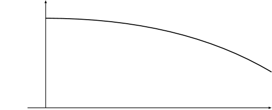
From Eqs. (2.124), (2.128), and (2.129) we obtain the field value of :
| (2.131) |
This should satisfy the COBE normalization in Eq. (2.116):
| (2.132) |
On the other hand, the COBE observations show the spectrum index as [82], while in the present new inflation model it is given by [84]
| (2.133) |
Therefore, we take in the following analysis assuming the coupling not be extremely small. (Notice that this justifies the assumption [see Eq. (2.130)].)
From the above relations, we calculate the inflation scale for given , and , which are shown in Fig. 2.12. The vacuum expectation value , the inflaton mass and the reheating temperature are found in Fig. 2.12, Fig. 2.14, and Fig. 2.14, respectively. From Fig. 2.14, we find that the new inflation model with the power indices and naturally offer the low reheating temperature . For the cases , we obtain GeV for the region – and –, respectively.


Now we turn to discuss the leptogenesis in this new inflation model. The ratio of the lepton-number density to the entropy density is again given by Eq. (2.49). Notice that the new inflation model with gives such a low reheating temperature as – (see Fig. 2.14) that the required amount of lepton asymmetry cannot be generated, and hence we discard this case.
The obtained lepton asymmetry for the cases and are shown in Fig. 2.16 and Fig. 2.16 by taking () and (), respectively. Here we have taken relatively smaller values of [see Eq. (2.89)] to obtain a wider allowed region, taking account of ambiguities in the FN model.
Interesting results are given for . (Here, we find that the condition excludes the regions and for the case .) From Fig. 2.14 and Fig. 2.16, we see that the sufficient lepton asymmetry can be generated for and with the low enough reheating temperature of –. In particular, for , the required lepton asymmetry is obtained for with low reheating temperature . Thus, we can avoid the overproduction of gravitinos for a wide range of gravitino mass – in this case.
On the other hand, when (), we find from Fig. 2.16 that the leptogenesis does not work well.


2.3.5 Topological inflation
In this subsection, we discuss the leptogenesis in a topological inflation. If the vacuum expectation value of the inflaton exceeds the gravitational scale, the inflaton potential of the new inflation in Eq. (2.122) becomes nothing but the inflaton potential for the topological inflation [87].
We adopt the SUSY topological inflation model proposed in Ref. [88]. The superpotential and Kähler potential in that model are given by
| (2.134) | |||||
| (2.135) |
where is the energy scale of the inflation and , , and are coupling constants of order unity. Hereafter, we take and to be real and positive by using the redefinition of the field and . These potentials possess symmetry; the charge of and are and , respectively, and () is odd (even) under the . This discrete symmetry is crucial to allow a topological defect (in this case, a domain wall) and hence to realize the topological inflation [87].
From Eqs. (2.98), (2.134) and (2.135) we find a SUSY-invariant vacuum:
| (2.136) |
where the scalar components of the supermultiplets are denoted by the same letters as the corresponding supermultiplets. The potential for the region , is written approximately as
| (2.137) |
Hereafter, we set assuming as we have done in the new inflation.
For and , the inflaton field is identified with the real part of and the potential around the origin is given by
| (2.138) |
where .
A topological inflation takes place if the vacuum expectation value of is of order of the gravitational scale [87]. It was shown in Ref. [89] that, in order for a topological defect (in our case, a domain wall) to inflate, its vacuum expectation value should be larger than the following critical value.
| (2.139) |
The slow-roll conditions in Eq. (2.104) are satisfied when and , where is expected to be of order of the gravitational scale. Hereafter, we take .
As for the decay of the inflaton , we assume that decays through the interactions in the Kähler potential as shown in Eq. (2.125), and hence the reheating temperature of the topological inflation is again given by with the decay rate in Eq. (2.126). Here, the inflaton mass in the true vacuum in Eq. (2.136) is estimated as
| (2.140) |
As in the other inflation models, the scale of this topological inflation is determined by (i) the -fold number , (ii) the density fluctuations and (iii) the spectrum index . The -fold number in the present model is estimated as
| (2.141) |
which should satisfy the present Hubble horizon scale in Eq. (2.114), while the COBE normalization in Eq. (2.116) requires
| (2.142) |
The spectrum index is again given by , and hence we take as in the new inflation model.


From the above relations, we can calculate the inflation scale and the mass , and hence the reheating temperature . We show the results in Fig. 2.18. Here, we have taken . A crucial deference between this model and the previous new inflation model is the reheating temperature. In this topological model, as shown in Fig. 2.18, relatively high reheating temperatures are obtained compared with those in the new inflation. This is because the large value of the vacuum expectation value . (See Eq. (2.126).)
Finally, we show the obtained lepton asymmetry in Fig. 2.18. Here, we have taken () and () as in the new inflation model discussed in the previous subsection. We can see that for the both cases enough lepton asymmetry is obtained for . On the other hand, the requirement of a low enough reheating temperature () is satisfied only in a small range of the coupling . (The lowest reheating temperature GeV is obtained for .) For , the spectrum index deviates from the scale invariant one as , and it will be testable in current and future satellite experiments on anisotropies of the cosmic microwave background radiation [90].
2.3.6 Production of right-handed neutrinos at preheating
Here, we briefly mention the production of right-handed neutrinos at preheating epoch, which was investigated in Ref. [74].
So far, we have assumed that the reheating process after the inflation occurs in such a way that energy density of the zero mode of the inflaton decays perturbatively into light particles. However, the heavy right-handed neutrinos might be predominantly produced nonperturbatively, through the parametric resonance [91, 92].
In Ref. [74], production of heavy right-handed neutrinos via preheating of fermion [92] was discussed, adopting a chaotic inflation with the inflaton potential . ( is the inflaton mass.) The point is that, if there is a Yukawa coupling between the inflaton and heavy fermion
| (2.143) |
then the effective mass of the fermion depends on time through the oscillating inflaton during the inflaton-oscillating period:
| (2.144) |
Therefore, the effective mass oscillates with time, and can even be zero if the amplitude of the oscillating inflaton is large enough, which is very crucial to produce very massive fermions heavier than the inflaton itself.
The production of the fermion crucially depends on the parameter
| (2.145) |
where denotes the initial amplitude of the inflaton oscillation. An efficient production of very massive fermions requires a large value of [74], and hence large enough initial amplitude . In the case of chaotic inflation, and can lead to .
The maximum mass of the produced fermion is given by [74]
| (2.146) |
If , the effective mass can vanish more than once [see Eq. (2.144)]222222Their numerical calculation shows [74] that the minimum of the inflaton amplitude during the first oscillation is given by . and the production of through parametric resonance occurs efficiently, whereas if otherwise the production is much less effective. The production continues during vanishing effective mass can be achieved. Namely, the production stops when the amplitude of the oscillating inflaton becomes below the following critical value:
| (2.147) |
The energy density of the inflaton at this time is thus given by . On the other hand, the energy density of the produced fermion at this frozen-out time is given by [74]
| (2.148) |
After that, i.e., for , the ratio of the energy density of the to the inflaton , , is fixed. From the above equations, this ratio is simply given by
| (2.149) |
Now let us identify the field to the right-handed neutrino . From above equation, the resultant lepton asymmetry after the reheating process of the inflation completes is given by
| (2.150) |
Thus, the baryon asymmetry is given by
| (2.151) |
where we have used Eq. (2.21).
Before closing this section, let us see what happens if we apply the above mechanism to the first one of the SUSY hybrid inflation models discussed in Sec. 2.3.3.a, where the inflaton has a Yukawa coupling to the right-handed neutrino. In this case, the parameter is estimated as
| (2.152) | |||||
Therefore, in the region we have studied, where the perturbative decay is kinematically allowed (), preheating takes place only through a narrow resonance, and hence only small fraction of the inflaton oscillating energy can be converted to heavy right-handed neutrinos via preheating. For the case of (), in the small coupling region and where [see Fig. 2.3], preheating mechanism might work effectively, although it requires another detailed analysis.
2.4 Leptogenesis from -dominant universe
In the previous sections, we have discussed the leptogenesis mechanisms by the decay of right-handed (s)neutrino, which is produced as a particle. However, there is a new possibility once we introduce the SUSY, that is, the condensation of the scalar component of the right-handed neutrino, [25].232323See also Refs. [24, 93], where the right-handed sneutrino is considered as an inflaton of the chaotic inflation. The lepton asymmetry is produced in the same way as the previous mechanisms, by the asymmetric decay of the right-handed “s”neutrino into leptons and anti-leptons. However, the thermal history of the universe in this scenario is quite different from the others. In this section,242424This section is based on the work in a collaboration with H. Murayama and T. Yanagida [26]. we investigate this scenario in detail. In particular, we mainly discuss the case in which the coherent oscillation of the right-handed sneutrino dominates the energy density of the universe before it decays. Remarkably, the amount of produced baryon asymmetry is determined almost only by the decay rate of the right-handed neutrino, whatever happened before the coherent oscillation dominates the universe. (Thus, the baryon asymmetry is independent of the details of the inflation !)
Furthermore, as a big bonus, the abundance of the gravitinos which are created in the reheating phase after inflation are diluted by the entropy production due to the decay of the coherent right-handed sneutrino, so that the cosmological gravitino problems can be avoided even when the reheating temperature of the inflation is higher than , in a wide range of the gravitino mass –. In particular, this dilution of the gravitinos has great advantages in the gauge-mediated SUSY breaking (GMSB) models [45].
We will also comment on the cosmic density perturbation caused by the quantum fluctuation of the right-handed sneutrino, which may be detected in the future.
2.4.1 Lepton asymmetry from -dominant universe
The main character in the present scenario is the right-handed sneutrino, . During inflation, it can acquire a large amplitude [25, 24, 93] if the Hubble expansion rate of the inflation is larger than the mass of the . (The mechanism which makes a scalar field develop a large initial amplitude during inflation will be explained in Sec. 3.2.2, in the context of the Affleck-Dime condensation.) Let us assume that there exists (at least) one right-handed neutrino with a mass lighter than , and that it develops a large expectation value during the inflation. Hereafter, we focus on the lightest right-handed sneutrino for simplicity. (Possible contributions from the heavier right-handed sneutrinos and will be discussed in Sec. 2.4.4.b.) It is assumed here that the potential for the right-handed neutrino is given simply by the mass term
| (2.153) |
We do not settle the initial amplitude of the at this stage, which will be discussed later. Because of the large amplitude of the , the lepton and Higgs doublets receive large masses, and the expectation values of their scalar components and vanish.
The evolution of the is as follows. After the end of the inflation, the Hubble parameter decreases with cosmic time as , and begins to oscillate around the origin when becomes smaller than the mass of the right-handed sneutrino . (.) Then, the coherent oscillation eventually decays when the Hubble expansion rate becomes comparable to the decay rate of . (.) As explained in Sec. 2.1, the asymmetric decay of into leptons and anti-leptons produces a net lepton asymmetry. The generated lepton number density is given by
| (2.154) |
where is the amplitude of the oscillation when it decays, and is given by Eq. (2.21).
The fate of the generated lepton asymmetry depends on whether or not the coherent oscillation of dominates the energy density of the universe before it decays [25]. Here, we focus on the leptogenesis scenario from the universe dominated by . (We will mention the case where does not dominate the universe in Sec. 2.4.4.d.) As we shall show soon, once the dominant universe is realized, the present baryon asymmetry is determined only by the properties of the right-handed neutrino, whatever happened before the dominates the universe. We first derive the amount of the generated lepton asymmetry just assuming that the dominates the universe, and after that we will discuss the necessary conditions of the present scenario.
Once dominates the universe before it decays, the universe is reheated again at by the decay of . The energy density of the resulting radiation, with a temperature , is given by the following relation;
| (2.155) | |||||
while the entropy density is given by [see Eq. (B.21)]
| (2.156) |
From the Eqs. (2.21), (2.154), (2.155) and (2.156), the ratio of the lepton number density to the entropy density is given by the following very simple form;
| (2.157) | |||||
Here, it is assumed that the decay of the occurs in an out-of-equilibrium way, namely, , so that the produced lepton-number asymmetry not be washed out by lepton-number violating interactions mediated by . As explained in Sec. 1.4, this lepton asymmetry is partially converted into the baryon asymmetry through the sphaleron effect:
| (2.158) | |||||
Therefore, as stressed previously, the baryon asymmetry in the present universe is indeed determined only by the decay temperature of the right-handed sneutrino (and the effective violating phase ). Thus it is independent of unknown parameters of the inflation such as the reheating temperature . Assuming the effective violating phase to be not too small, the empirical baryon asymmetry – is obtained by taking
| (2.159) |
2.4.2 Necessary conditions
So far, we have required the following two conditions;
-
(i)
dominates the universe before it decays.
-
(ii)
decays in an out-of-equilibrium way.
Let us first consider the easier one, the second condition (ii). By taking the in Eq. (2.159), the condition of the out-of-equilibrium decay is simply given by252525 The condition is formally equivalent to if we take the usual relation . However, this interpretation is not appropriate in the present case, since the universe is not radiation-dominant for . In any case, the condition Eq. (2.160) is necessary to avoid the thermal production of after the decay of the coherent .
| (2.160) |
Notice that this condition gives rise to a constraint on the Yukawa couplings , since the temperature is determined by the decay rate of the , and hence is related to the mass and couplings of . Actually, from Eq. (2.155) and , the following relation is derived:
| (2.161) |
Hence, it is found from Eq. (2.160) that Yukawa couplings of should be smaller than . (Possible explanations for the smallness of will be discussed in Sec. 2.4.4.a.)
Now let us turn to discuss the first condition (i). In order to discuss whether or not dominates the universe, it is necessary to consider the history of the universe before it decays. Here, we assume that the potential of the is “flat” up to the Planck scale, namely, the potential is just given by the mass term up to the Planck scale. (This may not be the case when the masses of the right-handed neutrinos are induced by a breaking of an additional gauge symmetry. We will discuss such a case in Sec. 2.4.4.d.)
Assuming the flatness of the ’s potential up to the Planck scale (i.e., only the mass term), the initial amplitude of the oscillation is naturally given by , since above the Planck scale the scalar potential is expected to be exponentially lifted by the supergravity effects [see Eq. (2.98)].262626Even though it is possible that has a larger initial amplitude (see, e.g., Ref [24, 93]), it depends on the scalar potential beyond the Planck scale, so that we do not discuss this possibility here. Then the energy density of when it starts the coherent oscillation is given by .
The rest of the total energy density of the universe at is dominated by (I) the radiation or (II) the oscillating inflaton , depending on the and the decay rate of the inflaton . (See Fig. 2.19.)
If [case (I)], the inflaton decay has already completed before , and the energy density of the radiation at is given by . In this case, the oscillating dominates the universe soon after it starts the oscillation and hence before its decay.
On the other hand, if [case (II)], the reheating process of the inflation has not completed yet at , and the inflaton is still oscillating around its minimum, whose energy density is given by . The ratio of the energy density of to that of the inflaton, , takes a constant value until either of these oscillations decays. Because the energy density of the radiation resulting from the inflaton decay is diluted faster than , the oscillating can dominate the universe if its decay rate is slow enough compared with that of the inflaton ; .272727More precisely, occurs for in case (II).
\psfrag{I}{\bf\huge(I)}\psfrag{II}{\bf\huge(II)}\psfrag{rho}{\huge$\rho$}\psfrag{R}{\qquad\huge$R$}\psfrag{HGC}{\large$H=\Gamma_{\chi}$}\psfrag{HM1}{\large$H=M_{1}$}\psfrag{GC}{\large$\Gamma_{\chi}$}\psfrag{GN1}{\large$\Gamma_{N_{1}}$}\psfrag{M1}{\large$M_{1}$}\psfrag{T}{\large$(T=$}\psfrag{TR}{\large$T_{R}$}\psfrag{TTR}{\large$(T=T_{R}$}\psfrag{TN1}{\large$T_{N_{1}})$}\psfrag{TM1}{\large$T_{M_{1}}$}\psfrag{rhoc}{\large$\rho_{\chi}\propto R^{-3}$}\psfrag{rhoN1}{\large$\rho_{N_{1}}\propto R^{-3}$}\psfrag{rhorad}{\large$\rho_{\rm rad}\propto R^{-4}$}\psfrag{MM}{\large$M_{1}^{2}M_{G}^{2}$}\includegraphics{Figs/N-dom.eps}
Therefore, the condition for to dominate the universe is just given by . In terms of the reheating temperature , it is
| (2.162) |
which is easily satisfied in various SUSY inflation models. (Recall that the SUSY inflation models in Sec. 2.3 naturally lead to –.) Thus, the present leptogenesis scenario from dominated early universe is almost automatic as long as the right-handed neutrino has suitable mass and couplings given in Eqs. (2.160) and (2.161).
2.4.3 Dilution of the gravitinos
A very attractive feature in the present “-dominant universe scenario” is the dilution of the gravitino due to the entropy production caused by the decay. We discuss this point in this subsection.
Let us first calculate the dilution factor of the entropy production caused by the ’s decay. It depends on the two cases discussed in the previous subsection, [case (I)] and [case (II)]. We first consider the latter case, [see Fig. 2.19 (II)]. At the time of inflaton decay (), the ratio of the energy density of to the entropy density is given by
| (2.163) |
where we have used and at . This ratio takes a constant value until the decays, since and are diluted at the same rate as the universe expands. Then at the time of the ’s decay, the energy density of the is converted to the radiation. The ratio of the energy density to the entropy density in the new radiation is given by
| (2.164) |
By equating the (just before the ’s decay) in Eq. (2.163) with the (just after the ’s decay) in Eq. (2.164), we obtain the dilution factor of the entropy production:
| (2.165) |
Next, we consider the case [case (I)]. In this case, the ratio takes a constant value after the starts its oscillation, i.e., for . This ratio is evaluated in the same way as Eq. (2.163):
| (2.166) |
where is the temperature at in the case (I), which is given by
| (2.167) |
Then the dilution factor at is obtained in the same way as in Eq. (2.165), which results in .
To summarize, the dilution factor is given by
| (2.170) |
where we have used the fact that () corresponds to ().
As discussed in Sec. 1.5, the abundance of the gravitino produced at the reheating epoch after the inflation is proportional to the reheating temperature of the inflation . Therefore, there are usually severe upper bounds on depending on the gravitino mass. However, in the present scenario, the number density of the gravitino is diluted thanks to the entropy production caused by the ’s decay, which was discussed just above. Namely, the constraint coming from the gravitino problems should apply, not to the reheating temperature , but to an effective temperature given by
| (2.173) | |||||
| (2.176) |
which is much below the original reheating temperature . Actually, for , the gravitino abundance which was originally produced at the reheating after primordial inflation is diluted and becomes comparable to the abundance which is produced at the “reheating” after ’s decay.
In the case of unstable gravitino, Eq. (2.173) means that the cosmological gravitino problem coming from the big-bang nucleosynthesis bounds can be avoided in a wide range of the gravitino mass –, even if the reheating temperature of the inflation is much higher than . (Recall that the is given by Eq. (2.167).) We should stress that the fact that such high reheating temperature is allowed makes it very easy to construct SUSY inflation models (see Sec. 2.3).
In the case of stable gravitino as well, we see from Eq. (2.173) that the overclosure problem can be avoided in a wide range of the gravitino mass. Actually, in our scenario, the relic abundance of the gravitino is obtained by dividing the original abundance in Eq. (1.28) by the dilution factor in Eq. (2.170):
| (2.177) | |||||
Therefore, the overclosure problem can be avoided almost independently of the reheating temperature , and a reheating temperature even higher than is possible for . Moreover, it is found from this equation that the present energy density of the gravitino is independent of the reheating temperature , in a very wide range of . Thus, we can predict the gravitino mass by requiring that the gravitino is the dominant component of the dark matter:282828Notice that with such a small gravitino mass as in Eq. (2.178), the problem of the decay of the next-to-lightest SUSY particle into LSP gravitino after the big-bang nucleosynthesis is also avoided [94, 48]. See Sec. 1.5.
| (2.178) | |||||
for . Here, we have taken the present matter density and [29].
Such a light (stable) gravitino as in Eq. (2.178) naturally exists in gauge-mediated SUSY breaking (GMSB) models [45]. The GMSB mechanism has been regarded as a very attractive candidate for the SUSY breaking, since it suppresses quite naturally the flavor changing processes, which are inherent problems in the SUSY standard model. It is remarkable that the gravitino with mass – becomes naturally the dominant component of the dark matter in the present scenario, independently of the reheating temperature for . This prediction comes from the fact that the present energy density of the gravitino is determined by the effective temperature (for ), while the decay temperature of the right-handed neutrino is fixed by the baryon asymmetry in the present universe [see Eq. (2.159)].
2.4.4 Remarks
We give several comments on the present scenario.
2.4.4.a neutrino masses
The first one is about the neutrino mass . Let us first rewrite the neutrino masses in terms of the three contributions from , and :
| (2.179) |
where
| (2.180) |
and the denote the Yukawa couplings of the neutrinos in the basis where mass matrices of heavy and light neutrinos are diagonal, which are defined in Eq. (2.18). Then we see that the contribution from satisfies the following relation:292929The last expression in Eq. (2.181) is nothing but the parameter in Eq. (2.34).
| (2.181) | |||||
Here, we have used the relation in Eq. (2.161). Therefore, it is understood that the mass scale of the neutrinos suggested from the atmospheric [10] and solar [11] (KamLAND [12]) neutrino oscillations, –, should be induced from the heavier right-handed neutrinos, and .
The relative hierarchy between the mass and couplings of and those of the and might be naturally explained by a broken flavor symmetry. For example, a broken discrete symmetry [95]303030The model here looks similar to the one in Sec. 3.3.1, but different from that. with a breaking parameter and charges , , and , , gives rise to the following superpotential;
where and are couplings. The above charge assignments for lepton doublets naturally lead to the realistic neutrino mass matrix including the maximal mixing for the atmospheric neutrino oscillation [76]. (See Sec. 2.3.2.) The overall mass scale of the right-handed neutrino is determined by . By taking , this model gives , , and hence .313131In terms of parameter, this corresponds to .
Recently, it has been shown [96] that the small mass and the couplings of the , required in the present scenario, naturally arise if the right-handed neutrino is a bulk field in higher dimensional theory.
2.4.4.b contributions from and
In the previous subsections, we have only considered the lightest right-handed sneutrino, . The heavier right-handed sneutrino can also develop a large amplitude during the inflation (if ) and it may produce lepton asymmetry in a similar way to the . However, it is found that the decay temperatures of the and cannot satisfy the out-of-equilibrium condition , since and must explain the mass scales of the neutrino oscillations. (In other words, if would also satisfy the condition , the mass scale for the neutrino oscillations could no longer be explained by the contributions from and [see Eq. (2.181)].) Therefore, even if the ’s decay produces additional lepton asymmetry, it is washed out and hence it cannot contribute to the resultant total lepton asymmetry.
2.4.4.c thermal effects
We should also comment on the effects of the thermal plasma, which might cause an early oscillation of the right-handed sneutrino before . (Notice that there is a dilute plasma with a temperature even before the reheating process of the inflation completes [28].) There are basically two possible thermal effects [97, 98]. (Those thermal effects will be also explained in detail in Sec. 3.2.3.)
First, when the temperature is higher than the effective mass for and , i.e., , the receives an additional thermal mass from the Yukawa coupling to and [97]. Thus, the field would start an early oscillation if the additional thermal mass becomes larger than the Hubble expansion rate before . However, even if receives the thermal mass, the ratio of the thermal mass to the Hubble expansion rate is given by
| (2.184) |
where we have used the relation given in Eq. (2.161). Therefore, we can safely neglect the above thermal effect as long as is a bit larger than .
There is also another thermal effect [98]. If the temperature is lower than the effective mass for and , i.e., , the evolution of the running gauge and/or Yukawa coupling constants which couple to them are modified below the scale . Thus, these running coupling constants depend on , and there appears an additional thermal potential for ;
| (2.185) |
where is a constant of order . However, again, it turns out that the effective thermal mass for is less than the Hubble expansion rate;
| (2.188) | |||||
and hence this thermal effect is also irrelevant to the present scenario.
2.4.4.d more general cases
So far, we have assumed that the initial amplitude of the ’s oscillation is . This can be realized when the right-handed neutrino has only the mass term up to the Planck scale. We have also assumed that the dominates the energy density of the universe before its decay. Here, we consider more general cases for completeness.
Let us assume that the masses of the right-handed neutrinos are dynamically induced by a spontaneously broken gauge symmetry, for example, by the symmetry, which is an attractive candidate for such a gauge symmetry as discussed in Sec. 1.1. We denote the chiral superfields whose vacuum expectation values break the by and . (We need two fields with opposite charges in order to cancel gauge anomalies.) Due to the -term and the -term coming from the superpotential which gives the right-handed neutrino masses, the scalar potential of the right-handed sneutrino is lifted above the breaking scale [25]. Therefore, the initial amplitude of the ’s oscillation at is given by .
The breaking scale of the gauge symmetry is model dependent. If it is broken at the Planck scale, , the discussion so far does not change at all.323232In this case, we need small couplings in order to explain the intermediate right-handed neutrino mass scale. For example, a superpotential with and gives the mass to the heaviest right-handed neutrino. Such a small Yukawa coupling could well be a consequence of broken flavor symmetries. On the other hand, if is below the Planck scale, the initial amplitude of the ’s oscillation is reduced and its energy density when it starts the oscillation is given by
| (2.189) |
Compared with the previous case (see Fig. 2.19), we can see that the initial energy density is much suppressed.
\psfrag{Ia}{\bf\Huge(Ia)}\psfrag{Ib}{\bf\Huge(Ib)}\psfrag{IIa}{\bf\Huge(IIa)}\psfrag{IIb}{\bf\Huge(IIb)}\psfrag{III}{\bf\Huge(III)}\psfrag{rho}{\huge$\rho$}\psfrag{R}{\qquad\huge$R$}\psfrag{HGC}{\large$H=\Gamma_{\chi}$}\psfrag{HM1}{\large$H=M_{1}$}\psfrag{GC}{\large$\Gamma_{\chi}$}\psfrag{GN1}{\large$\Gamma_{N_{1}}$}\psfrag{M1}{\large$M_{1}$}\psfrag{T}{\large$T=T_{R}$}\psfrag{TN}{\large$T=T_{N_{1}}$}\psfrag{TM}{\large$T=T_{M_{1}}$}\psfrag{c}{\Large$\chi$}\psfrag{r}{\Large rad.}\psfrag{N}{\Large$\widetilde{N_{1}}$}\psfrag{NN}{\huge$\widetilde{N_{1}}$}\psfrag{I}{\large$M_{1}^{2}|\widetilde{N_{1}}_{i}|^{2}$}\includegraphics{Figs/N-dom-generic.eps}
In Fig. 2.20, We show the behavior of the energy densities of the inflaton , the right-handed sneutrino and the radiation, for generic cases.333333For the reduced initial amplitude, the thermal effect from the potential becomes larger than the case of . However, it is still irrelevant as long as the coupling is small enough. [See Eq. (2.188).] Figure (Ia) and (Ib) represent the case of (), (IIa) and (IIb) represent the case of () and (III) represents that of (). Among them, (Ia) and (IIa) show the case of dominant universe, corresponding to (I) and (II) in Fig. 2.19, respectively. Figures (Ib), (IIb), and (III) represent the cases in which the coherent oscillation of the right-handed sneutrino does not dominate the energy density of the universe.
Let us first discuss the condition of the dominant universe, which was given by [Eq. (2.162)] for . Because of the smaller initial amplitude, the condition now becomes
| (2.190) | |||||
| (2.191) |
These conditions are summarized in Fig. 2.21. Notice that the cannot dominate the universe for [the case (III)].
\psfrag{Ia}{\bf\Large(Ia)}\psfrag{Ib}{\bf\Large(Ib)}\psfrag{IIa}{\bf\Large(IIa)}\psfrag{IIb}{\bf\Large(IIb)}\psfrag{III}{\bf\Large(III)}\psfrag{GC}{\Large$\Gamma_{\chi}$}\psfrag{TR}{\large$(T_{R})$}\psfrag{GN1}{\large$\Gamma_{N_{1}}$}\psfrag{M1}{\large$M_{1}$}\psfrag{TN1}{($T_{N_{1}}$)}\psfrag{TM1}{($T_{M_{1}}$)}\psfrag{Ni}{\Large$|\widetilde{N_{1}}_{i}|$}\psfrag{3M}{\large$\sqrt{3}M_{G}$}\psfrag{notNdom}{\large\bf\text@underline{not\,\,$\widetilde{N_{1}}$ dominant}}\psfrag{Ndom}{\Large\bf\text@underline{$\widetilde{N_{1}}$ \,\,dominant}}\psfrag{Ni3MGN1GC}{$|\widetilde{N_{1}}_{i}|>\sqrt{3}M_{G}\left({\displaystyle\frac{\Gamma_{N_{1}}}{\Gamma_{\chi}}}\right)^{1/4}$}\psfrag{Ni3MGN1M1}{$|\widetilde{N_{1}}_{i}|>\sqrt{3}M_{G}\left({\displaystyle\frac{\Gamma_{N_{1}}}{M_{1}}}\right)^{1/4}$}\includegraphics{Figs/N-dom-cond.eps}
Next we estimate the baryon asymmetry in the above general cases. It can be calculated in the same manner as before, and is given by, for each case,
| (2.195) |
where . Notice that the baryon asymmetry which was given in Eq. (2.158) does not change and independent of the initial amplitude as long as the dominant universe is realized [(Ia) and (IIa)].
Finally, we comment on the gravitino problem. The effective temperature of the cosmological gravitino problem, which was given by [Eq. (2.173)], is now given by
| (2.200) |
2.4.4.e cosmic microwave background (CMB) anisotropy from
Let us mention the cosmic density perturbation coming from the fluctuation of the initial amplitude of the right-handed sneutrino, , according to the recent study in Ref. [99].
In the present scenario, the CMB radiation we observe today has two origins; the inflaton and the right-handed sneutrino . Furthermore, if the Hubble expansion rate of the inflation is larger than the mass of the right-handed sneutrino , as we have assumed, the initial amplitude of the has a non-vanishing fluctuation during the inflation. Therefore, the CMB anisotropy also has two origins, the primordial fluctuations of and that of . If the completely dominates the energy density of the universe, the perturbation becomes adiabatic [100]. On the other hand, if the radiation coming from is negligible compared to that from , purely baryonic isocurvature perturbation is produced from . Particularly interesting is between these two cases (i.e., the region near the border line between the two regions (Ia)-(IIa) and (Ib)-(IIb)-(III) in Fig. 2.21), in which correlated mixture of the adiabatic and isocurvature fluctuation is generated, that can be observed in the current and future satellite experiments on the CMB anisotropies [90].
2.A -dominant universe from inflaton decay
In this appendix, we briefly discuss the case where the which are produced in inflaton decay dominates the universe before it decays. (This case was also discussed in Ref. [74].)
The baryon asymmetry produced by the decay in this case is the same as that of the -dominant universe (Sec. 2.4), and is given by Eq. (2.158):
| (2.201) |
which requires the decay temperature of the to be – for –.343434This point was not discussed in Ref. [74].
On the other hand, the condition for the to dominate the energy density of the universe in this case is derived as follows. The point is that the ratio , which is given by Eq. (2.48), takes a constant value until the time of ’s decay. Thus, the ratio of the energy density of the to that of the radiation at ’s decay is given by
| (2.202) | |||||
Thus, the dominant condition gives a lower bound on the as follows:
| (2.203) |
which is stronger than the out-of-equilibrium condition () for . Then using the relation in Eq. (2.161), we obtain a constraint on the Yukawa couplings:
| (2.204) |
If this is satisfied, produced from inflaton decay can dominate the energy density of the universe, and the produced baryon asymmetry is given by Eq. (2.201).
Chapter 3 Leptogenesis via flat direction
In the previous chapter, we have investigated various leptogenesis mechanisms in which lepton asymmetry is produced by the -violating, asymmetric decay of the heavy right-handed (s)neutrino into leptons and anti-leptons. In this chapter,111This chapter is based on the works with T. Asaka, M. Fujii and T. Yanagida [101, 95, 102, 103]. we will discuss a completely different leptogenesis scenario. The main character in this chapter is not a heavy right-handed (s)neutrino, but a flat direction scalar field including the charged lepton doublet . Actually, as we will see, most of the necessary ingredients for this scenario exist in the minimal supersymmetric standard model (MSSM), and basically it does not rely on any new physics beyond supersymmetry, the existence of small Majorana neutrino masses and inflation.
3.1 Overview
Affleck and Dine [27] proposed a completely new mechanism to produce cosmological baryon asymmetry, which is inherent in the SUSY framework. In the SUSY theories, there are many flat directions in the scalar potential which contain scalar quark (squark) and scalar lepton (slepton) fields, carrying baryon and/or lepton charges. During the inflation, such a scalar field (which will be denoted by ) can acquire a large vacuum expectation value along the flat direction, since the potential is flat. After the inflationary stage ends, the flat direction field starts a coherent oscillation. At this stage, if there exists baryon (or lepton) number violating operator in the scalar potential, field can have a nonzero phase rotational motion: , which means, a nonzero -number
| (3.1) |
is produced. (The dot denotes a derivative with time .) Since the field carries baryon (or lepton) number, this represents nothing but baryon (or lepton) number production.
Among various flat directions, the flat direction proposed by Murayama and Yanagida [25] is especially attractive and had been investigated in detail later as well [104, 105, 101, 95, 102, 103]. The most interesting point is that it is closely related to the neutrino physics. Actually, as we will see, the most important parameter which determines the present baryon asymmetry is the mass of the lightest neutrino, . Furthermore, the flat direction is very special among various flat directions, since it is free from a serious problem of the Q-ball formation.222We do not discuss the Q-ball problem in this thesis. For details and references, see, for example, Refs. [106, 102, 107].
Meantime, it has been pointed out [104, 97, 98] that the dynamics of a flat direction field is affected by thermal effects. Although production of baryon and/or lepton number usually takes place before the reheating process of the inflation completes, there is a dilute plasma even in this epoch. This dilute plasma can modify the scalar potential [97, 98], affect the dynamics of , and change (actually, suppress) the resultant baryon asymmetry.
In Sec. 3.2, therefore, we will perform a detailed analysis on the dynamics of the flat direction field , including all the relevant thermal effects, in order to calculate the amount of produced lepton (and hence baryon) asymmetry. We see that evolution of the field is indeed affected by the thermal effects, and that the produced lepton asymmetry is suppressed by those thermal effects. On the other hand, we will find a very interesting result: the amount of produced baryon asymmetry is almost independent of the reheating temperature , and is determined mainly by the mass of the lightest neutrino . We show that the empirical baryon asymmetry – predicts an ultralight neutrino – for a wide range of reheating temperature . In Sec. 3.3 we show some explicit models to explain such a small mass of the lightest neutrino.
Then we study in Sec. 3.4 what happens in this leptogenesis scenario via flat direction when we introduce a gauged symmetry. We will see that if the initial amplitude of the flat direction field exceeds the breaking scale, we can avoid the suppression of the lepton-asymmetry production due to the thermal effects.
Finally, in Sec. 3.5, we show that if we assume a very small mass of the lightest neutrino as suggested by the present leptogenesis mechanism, the rate of the neutrino-less double-beta decay can be predicted in a high accuracy.
A comment: we do not discuss other lepton-number carrying flat directions (see, e.g., early works in Refs. [108, 57], other general directions in Ref. [104], and a recent one in Ref. [109]) nor the case of multi-scalar manifolds [110]. Notice that the direction is special not only because it is a leptonic direction, but also because it is directly related to observable physics: the neutrino mass.
3.2 Lepton asymmetry from flat direction
In this section, we will discuss the dynamics of the flat direction field in detail and calculate the amount of generated lepton asymmetry.
3.2.1 The flat direction
Let us start by writing down the effective dimension-five operator in the superpotential
| (3.2) |
which induces neutrino masses after the neutral component of the Higgs field obtains its vacuum expectation value . Here, we have taken a basis where the neutrino mass matrix is diagonal. As we will see, the effective mass scales play crucial roles in the present scenario. Notice that they are directly related to the neutrino masses by the following equation:
| (3.3) |
Here and hereafter, we take , for simplicity.333This is the case for . Even for , the final lepton (and hence baryon) asymmetry changes (decreases) by a factor of .
We adopt the following scalar field as the Affleck-Dine flat direction [27] for leptogenesis, which was originally proposed in Ref. [25]:
| (3.8) |
where the factor is introduced to ensure the canonical kinetic term for . Here, we have chosen the neutral components of the and for illustration, which is always possible by using the gauge transformation. We also used an gauge rotation to make their phases to be the same.
There are three flat directions (). (See Appendix 3.A for more details.) Hereafter, we will suppress the family index for simplicity. As we will see later, it turns out that the relevant flat direction for the most effective leptogenesis corresponds to the first family . Thus, our flat direction field is parameterized by one complex scalar field, . We will use the same symbol to denote the supermultiplet corresponding to the scalar field , hereafter. Its superpotential is then given by
| (3.9) |
while the scalar potential is given by
| (3.10) |
Here, and are SUSY-breaking mass parameters,444Here, we have included the possible contribution from the -term, , which gives a mass term , in the mass . and the last term directly comes from the superpotential Eq. (3.9). Here and hereafter, we assume that the SUSY breaking is mediated by the gravity. Therefore, it is expected that and .
3.2.2 Initial amplitude
The potential for is -flat, and it is also -flat in the limit of . Thus, it is expected that the field can develop a large amplitude during the inflaton. It depends on the coupling between and the inflaton whether or not the field can have a large initial amplitude. Suppose that there are general nonminimal couplings of the field to the inflaton in the Kähler potential:
| (3.11) | |||||
where and are complex and real coupling constants, respectively, and the ellipsis denotes higher order terms which are irrelevant to the following discussion. During inflation, the energy density of the universe is dominated by the inflaton . Thus, the total energy density of the universe is given by , where is the Hubble parameter during the inflation and is the -component of the inflaton supermultiplet . Because of this nonzero energy density of , there appears additional SUSY-breaking effects during the inflation [104]. Using the scalar potential in the supergravity in Eq. (2.98), we obtain
| (3.12) |
where we redefined the phase of to include the phase of . A crucial observation here is that the field gets a large mass term of the order of the Hubble parameter. (We will call it a Hubble mass term.) In general, the coefficient of this Hubble mass term, , is expected to be order unity. If it is positive, therefore, the field is driven exponentially towards the origin during the inflation, and the present mechanism cannot work. (Notice that this would happen even if the Kähler potential is minimal, i.e., .) Hence, we will assume that it is negative, and hereafter take
| (3.13) |
with .
The negative Hubble mass term causes an instability of at the origin. From Eqs. (3.10) and (3.13), the minima of the potential are given by
| (3.14) | |||||
| (3.15) |
where we have used , . Since curvatures of the potential around the minimum along both the radius and phase directions are positive and of the order of the Hubble parameter , the flat direction runs to one of the four minima from any given initial value and is settled down it.
Here, we comment on another possibility that the flat direction field does not receive a mass term of the order of the Hubble parameter, which occurs with a Kähler potential of the no-scale type supergravity [111]. The evolution of the field in this case was discussed in Ref. [105], and it turns out that the initial amplitude is likely to be given by Eq. (3.14) in this case as well.
3.2.3 Evolution of the flat direction
Before discussing the detailed dynamics of the field, we first roughly describe the evolution of and note the relevant epoch for the leptogenesis. During the inflation, the field takes a large value as discussed in the previous subsection. After the end of inflation, the value of gradually decreases as the Hubble parameter decreases and then, at some time, the starts its coherent oscillation. As we will see, the net lepton number is fixed when the flat direction field starts the coherent oscillation.
Hereafter, we will assume that the net lepton number is fixed before the reheating process of the inflation completes, namely, during the epoch when the energy density of the universe is dominated by the oscillating inflaton . (This assumption will be justified after we calculate the amount of the generated lepton asymmetry in Sec. 3.2.4.)
3.2.3.a potential for
Let us first show the total effective potential for the flat direction field relevant to the leptogenesis:
| (3.16) | |||||
We explain each term in turn.
First of all, the -term potential and the SUSY-breaking terms give rise to the scalar potential at vacuum , which is given by Eq. (3.10).
Next, because the energy density of the universe is still dominated by the inflaton during the inflaton-oscillation epoch, the field receives additional SUSY-breaking terms caused by the finite energy density of :
| (3.17) |
This can be derived in the same way as Eq. (3.13). Recall that we have taken . We will call the second term Hubble -term.
Finally, the rests in Eq. (3.16) correspond to the thermal effects which we discuss now. The crucial point here is that the decay of the inflaton occurs during the coherent oscillation of , while it completes much later than the beginning of the oscillation. Thus, even in the oscillation period, there is a dilute plasma consisting of the decay products of the inflaton , although most of the energy density of the universe is carried by the coherent oscillation of . The temperature of this dilute plasma is given by [28]
| (3.18) |
Notice that in this dilute plasma the temperature decreases as , rather than as like in the usual radiation dominated universe.
This dilute plasma has crucial effects on the dynamics of the field [104, 97, 98]. There are basically two possible thermal effects. First, the fields which couple to are produced by the inflaton decay and/or by thermal scatterings if their effective masses are less than the temperature,
| (3.19) |
and hence they must be included in the plasma. Here, denote the Yukawa or gauge coupling constants between the flat direction and (we take real and positive). Therefore, the flat direction receives a thermal mass of order , if the condition Eq. (3.19) is satisfied. The induced mass term is given by [97]
| (3.20) |
where are real positive constants of order unity (see below). The summation means that only the fields in thermal plasma [i.e., whose couplings satisfy the condition Eq. (3.19)] can induce the thermal mass for .
We include all the couplings relevant for the flat direction in the SUSY standard model, i.e., the gauge couplings for the and gauge groups, and Yukawa couplings for up-type quarks and charged leptons. The couplings , which are redefined so that the effective masses for the fields become , are listed in Table. 3.1 with the coefficients of the thermal mass for . Among the gauge supermultiplets, the flat direction does not couple to one group which remains unbroken by the condensation of . Thus, there are one -like and two -like massive gauge multiplets as in the SUSY standard model. For the couplings of the charged leptons, we should be careful. The flat direction receives its thermal mass from only one linear combination of charged leptons. The effective Yukawa coupling is determined by the Yukawa couplings for the charged leptons and the mixing matrix among gauge eigenstates of the neutrinos. (Note that the relevant is the flattest direction which corresponds to the first family of mass eigenstates.) Taking large mixing angles both for atmospheric and solar neutrino oscillations suggested by the recent data [10, 11, 12], we find –. We will see in Sec. 3.2.4 that the Yukawa coupling for the up quark induces a relevant thermal effect, while other couplings turn out to be too large to satisfy the condition Eq. (3.19) in most of the parameter space.
| (coupling for ) | ( ) | |||
|---|---|---|---|---|
Next, there is another thermal effect which was pointed out in Ref. [98]. Along the flat direction, the gauge symmetry remains unbroken and hence gluons and gluinos are massless. Furthermore, the down type (s)quarks also remain massless since they have no direct coupling to the field. These massless fields produce the free energy which depends on the gauge coupling constant , and we obtain an effective potential at two loop level.555For the coefficient of this free energy, see, for example, Ref. [112]. At first sight, there seems no dependence on the field in this free energy. However, we can see this is not the case by means of the following arguments.
The evolution of the running coupling is given by
| (3.21) |
where and for fundamental representations . Notice that the evolution changes due to the decoupling when the scale passes through a mass of a field . Since the up type (s)quarks get large masses from the couplings to the field ( up, charm, top), they change the trajectory of the running at , as shown in Fig. 3.1.
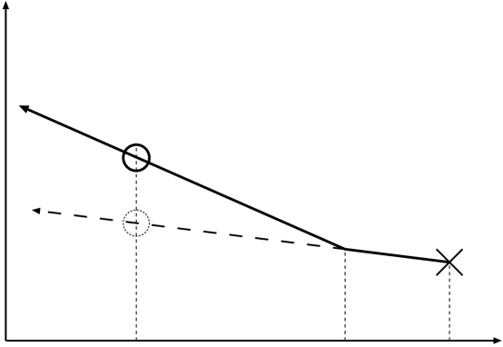
Hence, if , the running coupling depends on the value of the field:
| (3.22) |
where is the ultraviolet scale where is fixed. Then, there appears an additional potential through the modification of the gauge coupling constant in Eq. (3.22)
| (3.23) |
where is a constant which is a bit larger than unity666By using the free energy at two-loop order given in Ref. [112], is given by in the case of the flat direction. The author thanks Masaaki Fujii for helpful discussion. and . (We will omit the subscript for simplicity.) Hereafter, we take the factor to be unity since it does not change the result much.777At least the top Yukawa coupling always satisfies before the oscillation of . Thus, the resultant baryon asymmetry changes by only a factor of at most. [See Eqs. (3.38) and (3.45).]
3.2.3.b evolution of
Now we eventually obtain the total effective potential Eq. (3.16):
| (3.24) |
The evolution of is described by the equation of motion with this as
| (3.25) |
where the dot denotes a derivative with time. During the inflation, there is no thermal plasma and hence no thermal potentials. The vacuum expectation value of the field at this stage is given by Eqs. (3.14) and (3.15). Let us call the valley to which the field rolls down .
After the inflation ends, the inflaton starts to oscillate and its decay produces a dilute plasma. However, the potential is still dominated by Hubble-induced terms [in Eq. (3.17)] and term [in Eq. (3.10)] at the first stage of the oscillation. Thus, the flat direction field is trapped in the following minimum:
| (3.26) | |||||
| (3.27) |
This is because the curvatures around the minimum along both radius and phase directions are of the order of also in this period, and hence the field always catches up the instantaneous minimum [104].
Then, as the Hubble parameter decreases, the negative Hubble-induced mass term is eventually exceeded by one of the following three terms in the potential:888Here, we have compared instead of the potential terms themselves, since the evolution of is governed by the equation of motion Eq. (3.25).
| (3.28) |
As we show now, it is this time when the oscillation of starts. Let us denote the Hubble parameter at this time by . The evolution of the after depends on which term in Eq. (3.16) dominates the effective potential. There are basically three cases; the potential is dominated by (i) term, (ii) term, or (iii) term.
(i) First, if the potential is dominated by the term, the equation of motion Eq. (3.25) is given by
| (3.29) |
It is clear in this case that the field oscillates around the origin () and the amplitude of the oscillation damps as .
(ii) Second, when the potential is dominated by the thermal mass term , the equation of motion becomes
| (3.30) |
This equation can be solved analytically and the solution is given by
| (3.31) |
where and are constants and is the Bessel function. We see that the oscillates around the origin in this case as well. The time scale of the oscillation is and the amplitude of the oscillation is damped as .
(iii) The third case is given when the term dominates the potential. If we neglect the time dependence of , the damping rate of the oscillation amplitude due to such a flat potential, , can be estimated by using the virial theorem, and it is given by [113]. In the actual case, however, the potential itself gradually decreases with time as . We have numerically checked that the amplitude damps as with .
Thus, in any case, the field starts a coherent oscillation. Notice that, in all the above cases, the damping rate is faster than the rate before the beginning of the ’s oscillation ().
Now let us estimate the cosmic time when the field starts its oscillation, or equivalently the Hubble parameter at that time, . As we will see in Sec. 3.2.4, this oscillation time plays an important role to determine the final lepton asymmetry. is determined by the term which exceeds the Hubble mass term at first. (Therefore, again, there are three cases.)
(i) If the soft mass term dominates the potential at first, is just given by .
(ii) The case when the thermal mass term dominates at first is a bit complicated. Let us first consider a simple case in which there is only one field with a coupling . From Eqs. (3.19) and (3.28), it is found that the following two conditions must be satisfied in order to cause the ’s oscillation by the thermal mass term:
| (3.32) | |||||
| (3.33) |
where we have used the relations and . The meanings of these conditions are as follows. If the coupling is small enough, the can easily enter in the thermal plasma (), but the induced thermal mass for is smaller than the Hubble-induced mass at the beginning (). However, since the temperature decreases more slowly than the Hubble parameter () as the universe expands, the thermal mass eventually exceeds (). Then the ’s oscillation starts at the time when the condition Eq. (3.33) is satisfied. On the other hand, if is very large, the would-be thermal mass can be large enough to exceed the Hubble mass (). However, the thermal mass does not appear until the becomes small enough to satisfy . In this case the starts to oscillate at the time when the condition Eq. (3.32) is satisfied. Therefore, we find the Hubble parameter to be
| (3.34) |
It is easy to apply the above discussion to the case of more than one couplings. If there is another coupling which can satisfy the both conditions Eqs. (3.32) and (3.33) earlier than , the flat direction starts its oscillation earlier. Therefore, the Hubble parameter is given by999We assume here hierarchical couplings and neglect effects of the summation.
| (3.35) |
where
| (3.36) |
(iii) The third case is again given when the term dominates the potential at first. In this case, it is found from Eq. (3.28) that the oscillation time of the field is given by101010The running coupling here is obtained by solving the equation iteratively.
| (3.37) |
After all, the Hubble parameter at the time when the field starts its coherent oscillation is given by
| (3.38) |
where is given by Eq. (3.36). We stress here that the thermal effects always make the oscillation time earlier. (Notice that if there is no thermal effect, the oscillation time is just given by .) As we shall show soon, this “early oscillation” drastically affect the amount of the produced lepton asymmetry.
3.2.4 Lepton asymmetry
Now we are at the point to calculate the lepton asymmetry produced by the field. Since the field carries lepton charge, its number density is related to the lepton number density as
| (3.39) |
From Eqs. (3.16), (3.25) and (3.39), the evolution of is described by the following equation:
| (3.40) |
The production of the lepton asymmetry occurs as follows. Suppose that the original -term would vanish, i.e., . If this is the case, the flat direction is always trapped in one of the valleys induced by the Hubble -term [see Eq. (3.27)] during the both periods and , and the direction of the valley does not change with time. Therefore, there is no force which causes the motion of along the phase direction and no lepton-number asymmetry is produced (i.e., the right-hand side of Eq. (3.40) vanishes.) However, we have the original -term, and the phase of is kicked by the relative phase difference between and in Eq. (3.16). The phase of changes during its rolling towards the origin, because the Hubble parameter decreases and the direction of the true valleys changes with time. Therefore, the original -term, which corresponds to the first term in Eq. (3.40), plays a role of the source of the lepton asymmetry.
One might wonder if the Hubble -term, which corresponds to the second term in Eq. (3.40), gives a larger contribution to the lepton asymmetry since . However, since the almost traces one of the valleys determined mainly by the Hubble -term, in Eq. (3.40) is highly suppressed compared with . In fact, we have found numerically that the contribution of the second term in Eq. (3.40) is always comparable or less than that from the first term. Thus, we neglect the lepton asymmetry produced from the Hubble -term in our analytic calculation, for simplicity. By integrating Eq. (3.40), we obtain the resultant lepton number at the time ,
| (3.41) |
where denotes the scale factor of the expanding universe, which scales as in the universe dominated by the oscillation energy of the inflaton . We can see that the total lepton number increases with time as until the oscillation of starts (), since and hence in this stage.
On the other hand, after the starts its oscillation, the production of lepton number is strongly suppressed. This is because changes its sign rapidly due to the oscillation of , and also because the amplitude of ’s oscillation is damped as with . [See discussion around Eqs. (3.29)–(3.2.3.b).] Therefore, the net lepton asymmetry is fixed when the oscillation of starts. The generated lepton number at this epoch () is given approximately by
| (3.42) | |||||
where represents an effective violating phase. Here, we have used and . Recall that we have assumed that the production of net lepton asymmetry occurs before the reheating process of the inflation completes, i.e., where is the decay rate of the inflaton . Thus, the lepton number when the reheating process completes (, ) is given by
| (3.43) | |||||
Then, the lepton-to-entropy ratio is estimated as
| (3.44) |
when the reheating process of inflation completes. Here, we have used .
As explained in Sec. 1.4, this lepton asymmetry is partially converted into the baryon asymmetry through the sphaleron effect. Thus, after all, the present baryon asymmetry is given by
| (3.45) | |||||
From Eq. (3.45), we see that the baryon asymmetry is a monotonically increasing function of the scale . [Notice that the depends on as shown in Eq. (3.38).] Since is directly related to the neutrino mass as , this means that the baryon asymmetry becomes larger as the neutrino mass decreases. Therefore, as mentioned at the beginning of this chapter, the most effective flat direction corresponds to the lightest neutrino , i.e., the first family field .
The factor in Eq. (3.45) represents the suppression of the lepton asymmetry due to the thermal effects. When the ’s oscillation is caused by the thermal effects, i.e., , the production of lepton asymmetry stops earlier than the case without thermal effects, and hence the resultant baryon asymmetry becomes suppressed.
We should also note that the amount of the produced baryon asymmetry is proportional to the gravitino mass, . This is because the force which rotates the field along the phase direction comes from the SUSY-breaking -term . Thus, the resultant baryon asymmetry would be very much suppressed if the gravitino is light, like in gauge-mediated SUSY breaking models [45].111111If we introduce a gauged , however, the flat direction can produce enough lepton asymmetry even with a light gravitino. See Sec. 3.4. This is the reason why we have assumed gravity-mediated SUSY-breaking and .
Fig. 3.2 shows the contour plot of the produced baryon asymmetry in the – plane, given by the analytic formula Eq. (3.45).
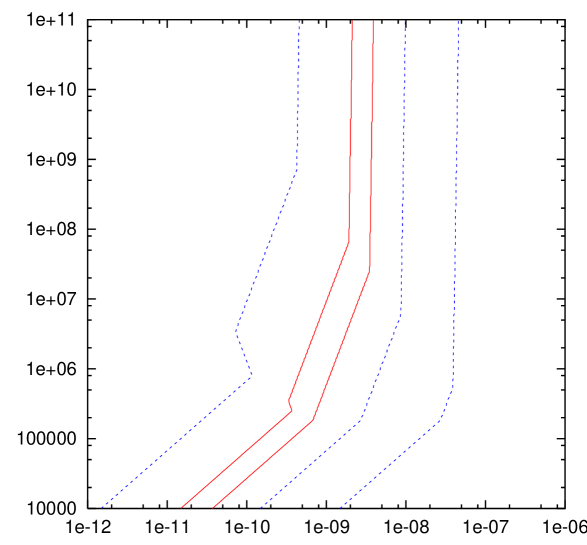
Here, we have taken , and , and we have used the relation . (Although the big-bang nucleosynthesis constraint on the gravitino abundance requires for , we have plotted the contour in Fig. 3.2 up to , keeping in mind that even can be allowed for a slightly heavier gravitino, say, . See Sec. 1.5.)
A remarkable observation here is that the present baryon asymmetry is determined almost independently of the reheating temperature for a wide range of . In particular, for a relatively high reheating temperature , the baryon asymmetry derived from the Eqs. (3.38) and (3.45) is given by the following simple from;
| (3.46) |
The reason why it is independent of the reheating temperature is that the oscillation time is determined by the thermal potential in the higher temperature regime and becomes proportional to the reheating temperature . [See Eq. (3.38).] Thus, the dependence is canceled out in Eq. (3.45).121212Precisely speaking, depends on through the running coupling even in this case. However, as can be seen in Fig. 3.2, this dependence is negligibly mild. Even in the lower reheating temperature region , where is determined by the thermal-mass term potential , dependence is still mild, i.e., . The “reheating-temperature independence” discussed here is a very attractive feature of the present mechanism since the produced baryon asymmetry crucially depends on in many other baryogenesis scenarios.
For the analytic calculation in Fig. 3.2, we have taken . It is expected that , say, –, unless there is an unnatural cancellation between and . Thus, it is found from Fig. 3.2 that the present baryon asymmetry in our universe – suggests an ultralight neutrino of a mass,
| (3.47) |
for and –.
remarks
Before closing this section, we give several comments. First, let us justify our assumption that the production of the lepton asymmetry stops before the reheating process of the inflation completes, namely, . We can see this condition is satisfied in all the parameter region in Fig. 3.2 by using the fact that is bounded from below, as shown in Eq. (3.38). For example, it is enough to show . By using , it is found that this condition is indeed satisfied for .
Next, let us investigate the behavior of Fig. 3.2 in more detail. Fig. 3.3 shows the dependence of the baryon asymmetry on the Yukawa coupling of the up quark. Notice that the up-quark Yukawa coupling is given by . In the previous figure 3.2, we have taken (and ). In Fig. 3.3, we have taken and for comparison.
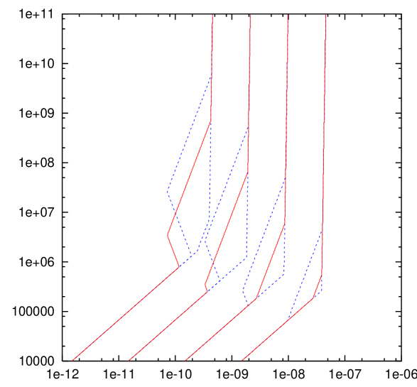
It is found that the final baryon asymmetry changes at most one order of magnitude. However, the dependence on the reheating temperature is still mild, and hence our conclusion does not change much.
Meantime, we can also see from Fig. 3.3 that the up-quark Yukawa coupling is the only coupling which can give a dominant contribution to the early oscillation of , since below this “up-quark Yukawa” region the oscillation is caused by the soft mass term (where ), while in the higher region the oscillation is caused by the thermal logarithmic term (where ). This is because other couplings are too large and the fields with those couplings cannot satisfy the condition .
We have also solved the equation of motion (3.25) numerically with the full scalar potential Eq. (3.16). The result is shown in Fig. 3.4, where the final baryon asymmetry is plotted. ( is given by Eq. (3.39), .) Here, we have taken , and . As for the initial condition, we have taken , and put the field at the minimum of the potential during the inflation. From Fig. 3.4 we confirm that the analytic estimation discussed above reproduces very well the result obtained by the numerical calculation.
Finally, we comment on the possibility to avoid the early oscillation caused by the thermal effects discussed in this section, which has been recently pointed out in Ref. [114]. The point is that, if the scale of the inflation is very low, the Hubble parameter during the inflation can be below the which is given by Eq. (3.38). If , our (implicit) assumption that the Hubble parameter of the universe gradually decreases from to breaks down. What happens in this case is that the flat direction field starts its oscillation just after the inflation ends, i.e., at . Thus lepton asymmetry is also fixed at this time. The final baryon asymmetry is then given by replacing in Eq. (3.45) with :
| (3.48) |
It was shown [114] that is indeed satisfied for very low and high enough reheating temperature , e.g, and –. For example, in an extreme case where and (sudden reheating), baryon asymmetry is given by [114]
| (3.49) |
Thus the empirical baryon asymmetry can be explained even with in this extreme case.
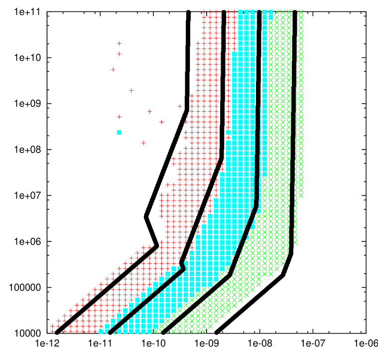
3.3 Some models
In Sec. 3.2.4 we have shown that the baryon asymmetry in the present universe predicts the mass for the lightest neutrino in a narrow region, –. Together with the neutrino masses required to solve the solar [11] and atmospheric [10] neutrino anomalies, this suggests a very large mass hierarchy between the lightest and the heavier two neutrinos.
Although the present leptogenesis mechanism via direction does not rely on the origin of the effective operator Eq. (3.2), it is natural to consider the seesaw mechanism [13] as the origin of that operator. In this case, the effective mass scale is related to the masses of the right-handed neutrinos . Then, one might wonder if the discussion so far is reliable, since successful leptogenesis requires the effective mass scale to be far beyond the Planck scale , i.e., . Here, we first comment on this point. In the framework of the seesaw mechanism, the neutrino masses are given by Eq. (2.2):
| (3.50) |
where we have rotated the Yukawa coupling so that the neutrino mass matrix becomes diagonal [see Sec. 2.1 and Eq. (2.18)]. Then, from Eqs. (3.3) and (3.50) we obtain
| (3.51) |
Therefore, the large mass scale (or equivalently small neutrino mass ) can be obtained by taking the Yukawa couplings to be small, keeping the masses of the right-handed neutrinos to be below the Planck scale.
Nonetheless, the reader might still consider that the mass scale is too large. In other words, the mass of the lightest neutrino – might seem to be too small, compared with the masses of the two heavier neutrinos, – suggested from the recent neutrino oscillation experiments [10, 11, 12]. In this section, we propose some models in which such an ultralight neutrino (or large mass scale ) can be naturally implemented.
3.3.1 Model for the ultralight neutrino with a broken discrete symmetry
Here, we show an explicit model based on a Froggatt-Nielsen (FN) mechanism [68], in which the required large mass hierarchy is naturally obtained. We adopt a discrete as the FN symmetry instead of a continuous . We see that the discrete symmetry is crucial to produce the required large mass hierarchy in the neutrino sector. To see this, let us first recall the case of the continuous , which is described in Sec. 2.3.2. In that case, the mass matrix of the neutrino in Eq. (2.79) gives rise to a mild hierarchy
| (3.52) |
and hence it cannot explain the large hierarchy required in the present scenario. To change the above point, we suppose that the broken FN symmetry is not a but a discrete symmetry with . Then, the mass matrix for the right-handed neutrino changes into the following form;
| (3.56) |
Here, we have assumed . Notice that the Majorana mass for is no longer suppressed by the power of , which is a basic point to yield an extremely small neutrino mass . Although the mass matrix is modified, the structure of the neutrino mass matrix looks similar to the original one:
| (3.66) | |||||
| (3.70) |
However, in spite of the large components of the mass matrix, we see that one of the mass eigenvalue of this mass matrix strongly suppressed as . (This suppression is also understood directly by taking the determinant of the above mass matrix.) Thus, the required large mass hierarchy between and can be naturally obtained by taking ().
Notice that the neutrino mass matrix Eq. (3.66) can still lead to a large – mixing angle. The mass hierarchy of the charged leptons also remains unchanged.131313This is because the charges of the Yukawa couplings of the charged leptons are smaller than , . Hence, this model preserves all the desirable features in the continuous model, explaining the mass of the ultralight neutrino as well.
\psfrag{r}[r][l][1.0][90]{$r=\displaystyle\frac{\delta m^{2}_{\rm sol}}{\delta m^{2}_{\rm atm}}$}\psfrag{mn1}[t][b][1.0][0]{$m_{\nu{1}}\,\,[~{}\mbox{eV}~{}]$}\includegraphics{Figs/Z6.eps}
To demonstrate our point, we randomly generate couplings and . Namely we calculate the mass matrix for neutrinos, taking the magnitudes of the couplings and to be in a range – and their phases to be – . We also take – randomly.141414A similar calculation was done in Ref. [77], where they adopted the continuous U model. From the obtained neutrino mass matrix, we calculated the mass eigenstates and the mixing matrix ,151515The matrix is defined in Sec. 2.1. and then required the parameters , , , and to be consistent with the data of neutrino-oscillation experiments [10, 11, 12]. Here, we take large-angle MSW solution to the solar neutrino deficits, since it is the only solution allowed by the recently announced KamLAND results [12], and adopt the following constraints [10, 115]:
| (3.71) |
We also required
| (3.72) |
to satisfy CHOOZ limit [116]. Fig. 3.5 shows the obtained mass of the lightest neutrino, . We can see that an ultralight neutrino of mass – eV is naturally obtained.
3.3.2 Large effective masses for right-handed neutrinos
In Sec. 3.3.1, we have shown a model in which an ultralight neutrino with mass – can be naturally implemented. Here, we discuss another possibility. The point is that the large effective mass scale is required only during the leptogenesis, not necessarily at the true vacuum. Therefore, if the effective masses of the right-handed neutrinos in the early universe are dynamical values and they are different from the values in the true vacuum, we might naturally obtain a large effective mass scale during the leptogenesis.
Suppose that the right-handed neutrino masses are given by a vacuum expectation value of some field with a superpotential
| (3.73) |
which gives . If takes a large value during the leptogenesis, therefore, can be much larger than the values in the true vacuum. To demonstrate this point, let us consider that the field is responsible to the Peccei-Quinn symmetry breaking [117]. Then, as we will see, there automatically exists a flat direction containing the field. The field can have a large value as during the inflation whereas it has a vacuum expectation value of in the true vacuum. Here, the Peccei-Quinn breaking scale is constrained by laboratory experiments, astrophysics, and cosmology as – [118].
We consider the following superpotential for the Peccei-Quinn symmetry breaking sector:
| (3.74) |
where is a coupling constant, and , , and are supermultiplets which are singlets under the standard-model gauge groups, which have , , and Peccei-Quinn charges, respectively. From Eq. (3.74) we see that there exists a flat direction . We parameterize this direction by the scalar field , which is called “saxion”. This saxion receives a soft SUSY breaking mass of , and the and have vacuum expectation values of the order of .161616We assume here that the soft SUSY breaking masses for and are almost the same, i.e., ().
Along this flat direction the field can have a large value during the inflation, if the additional SUSY breaking effects during the inflation induce a negative mass squared for (see Sec. 3.2.2). The initial value of is then expected to be , since the supergravity effects prevent the field from running over [see Eq. (2.98)], while the initial value of the field is given by .
In order to fix the mass scale at the true vacuum, let us take the mass of the lightest neutrino to be for a representative value, with which the hierarchy of the neutrino masses becomes mild. Then the scale is given by
| (3.75) |
Here, we have used and at the true vacuum . Although this scale at the true vacuum is too low to produce the enough baryon asymmetry (see Fig. 3.2), the large initial value of , gives rise to
| (3.76) |
For such a high scale , the evolution of the field is completely free from the thermal effects and the early oscillation can be avoided, even if the reheating temperature is as high as .171717This can be seen by calculating the oscillation time in Eq. (3.38) with .
The baryon asymmetry is then obtained by using Eqs. (3.45) and (3.76) as
| (3.77) |
where we have used . This shows that too large amount of the lepton asymmetry is produced. However, this asymmetry is sufficiently diluted, since there exists substantial entropy production by the decay of the saxion .
The saxion begins the coherent oscillation with the initial amplitude at , just after the production of the lepton asymmetry ends. The oscillation energy at that time is given by . When the reheating process of the inflation completes, the ratio of to the energy density of the radiation of the universe is estimated as
| (3.78) |
Notice that decreases at the rate as the universe expands, while decreases as . Therefore, the oscillation energy of the saxion dominates the energy of the universe soon after the reheating process completes. Here, it is useful to take the ratio of to the entropy density ,
| (3.79) |
which takes a constant value until the saxion decays.
This energy density of the saxion is transferred into the thermal bath when it decays. Here, it should be noted that the saxion might decay dominantly into two axions. If it is the case, the extra energy of the axion at the BBN epoch raises the Hubble expansion of the universe, which leads to overproduction of 4He. To avoid this difficulty, the branching ratio of the saxion decay into two axion should be smaller than about 0.1. Here, we simply assume this is the case.181818 This is realized when . Then, the saxion decays dominantly into two gluons with the decay rate
| (3.80) |
Through this decay the universe is “reheated” again, and its reheating temperature is estimated as
| (3.81) |
Notice that the saxion decay takes place far before the beginning of the Big-Bang Nucleosynthesis, and hence is cosmologically harmless.
The saxion decay increases the entropy of the universe by the rate
| (3.82) | |||||
Because of this entropy production by the saxion decay, the primordial baryon asymmetry Eq. (3.77) is also diluted by the rate . Then the present baryon asymmetry is given by
| (3.83) |
Notice that the present baryon asymmetry is independent of the reheating temperature , while it depends on the Peccei-Quinn scale . We see that the desired baryon asymmetry is obtained even with the lightest neutrino mass of for .
Finally, we comment on the cosmological consequences of this model.
(i) The entropy production by the saxion in Eq. (3.82) ensures that we are free from the cosmological gravitino problems, since the number density of gravitinos produced at the reheating process is diluted by the rate .
(ii) This model does not suffer from the cosmological problem of the “axino”, which is a fermionic superpartner of the axion. The axinos are produced in the reheating process by the thermal scatterings and may lead to a cosmological difficulty [119]. However, in this model, the interaction of axino at the reheating epoch is suppressed by , not by , and hence the production of axino is less effective. Furthermore, the entropy production by the saxion decay dilutes the axino abundance. Thus, the axino becomes completely cosmologically harmless in this model.
(iii) The reheating temperature of the saxion decay Eq. (3.81) is high enough to thermalize the lightest SUSY particles (LSPs) if the mass of the LSP is less than , and hence the stable LSP can be a dominant component of the dark matter.
3.4 Effects of the gauged symmetry
In Sec. 3.2, we found a very interesting aspect of the leptogenesis via flat direction, the “reheating temperature independence of the cosmological baryon asymmetry.” The resultant baryon asymmetry is almost determined by the mass of the lightest neutrino (and the gravitino mass), and hence we can predict the mass of the lightest neutrino as from the observed baryon asymmetry.
In this section, we discuss the effects of gauging the symmetry on the leptogenesis via the flat direction. As mentioned in Sec. 1.1, the absence of gauge anomaly automatically requires three families of right-handed neutrinos, and the breaking of symmetry naturally gives rise to the heavy Majorana masses of these right-handed neutrinos, which explains the tiny neutrino masses via the seesaw mechanism.
Below the breaking scale, the behavior of the scalar potential of the field does not change much from the one discussed in Sec. 3.2. Therefore, if the breaking scale is larger than the initial value of field obtained in Sec. 3.2.2,
| (3.84) |
the amplitude of the field is always smaller than the breaking scale, and the dynamics of the field is basically the same as the one discussed in Sec. 3.2. Hence, the resultant baryon asymmetry reduces to the one obtained in Sec. 3.2.4 [see Eq. (3.45) and Fig. 3.4]. We will call this case “-term stopping case.”
On the other hand, if , the field develops its initial value as large as the breaking scale. At this scale, the potential of the flat direction can be lifted by the effect of the -term [106]. (We denote this case by “-term stopping case.”) As we shall show in this section, the dynamics of the field is drastically changed in this -term stopping case. Actually, the obtained baryon asymmetry is much larger than the case without a symmetry, and hence than the -term stopping case.
It is interesting that the resultant baryon asymmetry in the -term stopping case linearly depends on the reheating temperatures of inflation, but it is completely independent of the gravitino mass. This is totally an opposite situation to the result obtained in Sec. 3.2, in which the final baryon asymmetry is almost independent of the reheating temperatures of inflation and linearly depends on the gravitino mass [see Eq. (3.45) and Fig. 3.4]. This “gravitino-mass independence of the cosmological baryon asymmetry” provides us a great advantage in gauge-mediated SUSY breaking scenarios [45].
3.4.1 The model
In order to discuss the effect of the gauge symmetry, we should investigate the breaking sector, which gives the masses of the right-handed neutrinos. To demonstrate our point, we use the following superpotential:
| (3.85) |
where, , , are coupling constants and we assume . , and are singlets under the MSSM gauge groups and they carry the charges of , and , respectively. is the the breaking scale of the symmetry. Here and hereafter, we take the couplings , , and , to be real, by field redefinitions. We will omit the family indices, since the “effectively flat” direction relevant for the present baryon asymmetry is again given by the flattest flat direction, .
The shape of the superpotential in Eq. (3.85) is the same as that of the SUSY hybrid inflation discussed in Sec. 2.3.3.a.191919The superpotential in Eq. (3.85) is also similar to the one in the model in Sec. 3.3.2. However, the model adopted here is different from that, since the symmetry here is gauged, while in Sec. 3.3.2 the Peccei-Quinn symmetry is global. Actually, If the field in Eq. (3.85) develops a large expectation value and the energy density of the universe is dominated by the vacuum energy , hybrid inflation takes place. Here, however, we assume that the breaking sector in Eq. (3.85) is not directly related to the inflation, and discuss the effects of this on the dynamics of the flat direction.
As we have shown in Sec. 3.2.2, the Kähler potential must have non-minimal couplings of the field to the inflaton , since otherwise the field gets a large positive mass term of the order of the Hubble parameter and it is driven exponentially towards the origin during inflation [104]. We assume that there are also non-minimal couplings of other fields to the inflaton in the Kähler potential:
| (3.86) | |||||
where and are complex and real couplings of order unity, respectively, and denotes , , , , , , and . Then, the full scalar potential relevant to the flat direction field is given by 202020Here, we take assuming a positive Hubble-order mass term for the field. This is necessary in order to avoid a contamination of to the flat direction. We have checked both analytically and numerically that the contamination of the field becomes relevant only after the , and hence the following discussion is not affected much by the contamination.
| (3.87) | |||||
where and , and we redefined the phase of . is the gauge coupling constant of the . represents SUSY breaking terms in the true vacuum. All fields denote the scalar components of the corresponding superfields. Here, we omit the potential coming from thermal effects, which will be discussed in Sec. 3.4.4.
The scalar potential in Eq. (3.87) is so complicated that it seems very difficult to solve the dynamics of the relevant fields. Fortunately, however, we only need to know the shape around the minimum of this potential, if the curvatures around the bottom of the potential are as large as the Hubble parameter during inflation. This is because all the scalar fields, which have masses as large as the Hubble parameter, settle down at the bottom of the potential during inflation and trace this potential minimum in the subsequent evolution. Therefore, we first find out the relations to minimize the potential in Eq. (3.87). Though this is also a very hard task because of the complexity of the potential, one can find out the minimum of the potential at least when and are satisfied. From Eq. (3.87), we find the approximate minimum of -terms for ,
| (3.88) |
Notice that the curvatures associated with these three relations are of the order of the breaking scale , and hence these relations hold as far as . By using these relations, we can reduce the scalar potential in Eq. (3.87) to the following one:
| (3.89) | |||||
where . Here and hereafter, we assume for simplicity. (This corresponds to in the previous analysis. See Eq. (3.17).)
One may wonder why the “flat” direction field can develop a large expectation value in spite of the presence of the -term. This is because the field shifts and absorbs the -term potential:
| (3.90) |
The curvature associated with this relation is also of the order of the breaking scale. Then we get the following effective potential:
In the following discussion, we assume and that the relations in Eq. (3.88) and in Eq. (3.90) are satisfied during the leptogenesis works. Although the approximation we have made here is crude, we will justify by a numerical calculation that the effective potential in Eq. (LABEL:EQ-Vfinal) is valid at least for the following discussion.
As we will see later, the third term in Eq. (LABEL:EQ-Vfinal),
| (3.92) |
which depends on the phase of , plays a crucial role in the -term stopping case. We will call this term “Hubble -term.” (This corresponds to the Hubble -term in Eq. (3.17) in the previous analysis.)
3.4.2 Initial amplitude and initial phase
In this subsection, we discuss the evolution of the field during the inflation.
3.4.2.a initial amplitude
First, we discuss the amplitude of the field. Let us first investigate the potential in the range . In this range, the field in Eq. (3.90) is expanded into the following form:
| (3.93) |
By substituting Eq. (3.93) into Eq. (LABEL:EQ-Vfinal), we get the effective potential for in the following form:
| (3.94) | |||||
where the ellipsis denotes higher order terms in . Here, corresponds to the mass scale which was denoted by the same symbol in Sec. 3.2. (The mass of the right-handed neutrino in the present model is given by .) Recall that it is related to the neutrino mass as .
The scalar potential in Eq. (3.94) is nothing but the potential obtained in Eq. (3.16) in the previous analysis, with some modifications.212121As we mentioned, the potential terms coming from thermal effects will be discussed in Sec. 3.4.4. However, there is an important difference in the Hubble-induced SUSY breaking mass terms. Since there appears an extra Hubble mass term, we need the following condition in order that the field develops a large expectation value during the inflation:
| (3.95) |
If this is not satisfied, the field is driven toward the origin during the inflation, and the leptogenesis cannot work. In the following discussion, we assume that the above condition is satisfied. Then the field has a negative Hubble mass term at least in the range of .
Now let us discuss the scale where the flat direction is lifted. If the balance point between the negative Hubble mass term and the -term potential in Eq. (3.94) is below the breaking scale , the field is stopped at this balance point,
| (3.96) |
This is the condition for the “-term stopping case.” In this case, the evolution of the field and the amount of the generated baryon asymmetry result in the same conclusions as discussed in Sec. 3.2.
On the other hand, if the condition
| (3.97) |
is satisfied, the field can develop its expectation value as large as . In this case, we can stop the field below the balance point by using the -term potential. This is very crucial to enhance the final baryon asymmetry in the -term stopping case. To see this, let us discuss what happens if the field develops its value as large as the breaking scale . At this scale (i.e., ), the expansion of the field given in Eq. (3.93) becomes invalid and above this scale we must use another expansion of the field as follows:
| (3.98) |
One might wonder whether the above expansion is reliable, since Eq. (3.90) is based on Eq. (3.88), which may not be valid for . Here, we first derive the conditions to fix the field at the scale during the inflation, assuming this expansion is effectively valid at least for . We will justify later the validity of the obtained conditions by numerical calculations.
By substituting the expansion Eq. (3.98) into Eq. (LABEL:EQ-Vfinal), we obtain the following Hubble-induced mass term:222222 Here, we assume . If this is not the case, we must include the Hubble mass term coming from the coupling of the right-handed Majorana neutrino to the inflaton, the last term in Eq. (LABEL:EQ-Vfinal).
| (3.99) |
Therefore, the field can have a positive Hubble mass term for , if
| (3.100) |
Therefore, if this condition is satisfied, the field cannot develop its expectation value above the scale , and hence it is fixed at the breaking scale during the inflation.
To summarize, the field, and hence and fields as well, are stopped at the breaking scale during the inflation, if the following conditions are satisfied,
| (3.101) |
These are the conditions for the -term stopping case.
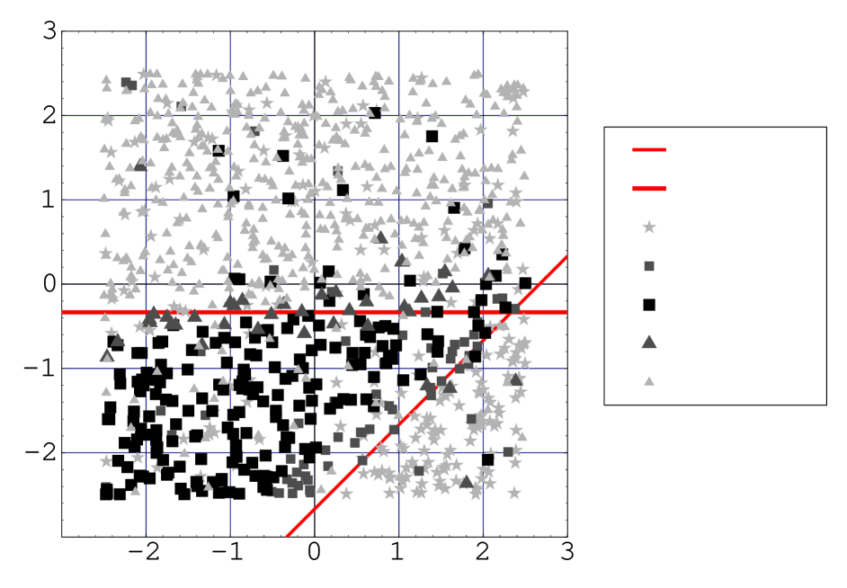
In order to check the reliability of the conditions in Eq. (3.101), (especially that of the last condition ,) we have numerically solved the coupled equations of motions
| (3.102) |
for the relevant fields , , , and , using the full scalar potential in Eq. (3.87). We show the result in Fig. 3.6, where the amplitude of the field at the end of the inflation is plotted in – plane. Here, we have taken and , and hence the second condition is satisfied.
3.4.2.b initial phase
Now let us turn to discuss the phase of the field at the end of the inflation, which is crucial to estimate the resultant lepton asymmetry.
First, in the -term stopping case, the amplitude of the field is fixed at . An important point here is that the curvature around the valley of the Hubble -term potential in Eq. (3.92) (which we denote by the symbol ) is of the order of the Hubble parameter in this case. This can be seen from the following relation:
| (3.104) | |||||
Therefore, as discussed in Sec. 3.2, the phase of the field settles down at the bottom of the valley of the -term potential during the inflation, and hence the Hubble -term cannot supply a torque to rotate the field. In this case, the relevant torque for the field only comes from the ordinary -term potential proportional to the gravitino mass. As stressed in Sec. 3.2.4, this leads to a suppression of the baryon asymmetry in gauge-mediation models with a small gravitino mass.
However, if the conditions in Eq. (3.101) are satisfied, namely, in the -term stopping case, the curvature of the potential along the phase direction is smaller than the Hubble parameter during the inflation:
| (3.105) | |||||
In this case, therefore, there is no reason to expect that the field sits down at the bottom of the valley of the -term potential in Eq. (3.92) during the inflation. In other words, unless there is an accidental fine tuning of the initial phase of the field, it is generally displaced from the bottom of the valley of this -term potential when the inflation ends.
Therefore, the -term potential kicks the field along the phase direction when the Hubble parameter becomes comparable to the curvature along the phase direction . As we will show in the next subsection, this phase rotation caused by the Hubble -term is very crucial to enhance the final baryon asymmetry.
3.4.3 Lepton asymmetry
Now let us discuss the dynamics of the field and calculate the resultant lepton asymmetry in the present model. In the -term stopping case, the amplitude of the field is always smaller than the breaking scale [see Eq. (3.96)] and the evolution of the field is determined by the effective potential in Eq. (3.94) plus thermal effects, which we have investigated in Sec. 3.2. Thus, the resultant baryon asymmetry is given by Eq. (3.45) (or Fig. 3.4).
We turn to the -term stopping case. As discussed in the previous subsection, the amplitude of the field at the end of the inflation is given by
| (3.106) |
and the phase of the field is generally displaced from the bottom of the valley of the Hubble -term potential.
After the end of the inflation, the field value of the field takes an almost constant value for a while. Then the Hubble -term in Eq. (3.92) kicks the field along the phase direction when the Hubble parameter becomes comparable with the curvature:
| (3.107) |
Thus, the Hubble parameter at this time is given by
| (3.108) |
At this time, the phase of the field, , starts to oscillate around the bottom of the valley of the Hubble -term potential. At the same time, the amplitude of the field, , starts to decrease according to the following equation:
| (3.109) |
which is the balance point between the negative Hubble mass term and the potential.
Since the phase of the field starts its oscillation at , it has already had a large acceleration along the phase direction before it starts coherent oscillation along the radius direction around the origin when . This is determined by thermal effects, soft SUSY breaking mass term and -term in the same way as in Sec. 3.2. Here, we have assumed that , which we will discuss in Sec. 3.4.4.
In Fig. 3.8 and Fig. 3.8, we show the evolution of the amplitude and the phase of the field obtained by numerical calculations, respectively. In these figures, is the cosmic time in the matter dominated universe . We see from these figures that the evolution of the field is well explained by above arguments.
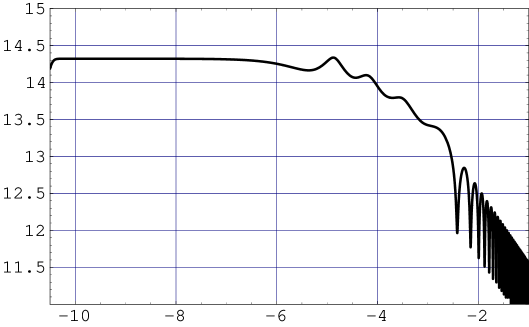
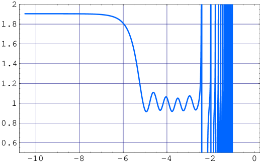
We are now at the point to estimate the baryon asymmetry. From the equation of motion (3.25), the evolution of the lepton asymmetry is given by
| (3.110) |
where we have used for . This can be easily integrated and we obtain the lepton number at time as
| (3.111) |
Before the ’s oscillation, i.e., for , the amplitude of the field decreases as and the sign of in Eq. (3.111) changes with time scale. (See Fig. 3.8 and Fig. 3.8.) Therefore, we see from Eq. (3.111) that the total lepton number oscillates with time scale with almost constant amplitude, since in this period.
Then, the total lepton number is fixed when the field starts its coherent oscillation around the origin at , since the amplitude of the field decreases as fast as and the integrand of Eq. (3.111) decreases as after the oscillation. The lepton number density at time is then given by
| (3.112) | |||||
where is the effective -phase. By using Eq. (3.43), the final lepton asymmetry is given by
| (3.113) |
Here, we have used the fact that the field starts its oscillation before the reheating process completes, i.e., , which was verified in Sec. 3.2.4. Notice that the resultant lepton asymmetry is independent of the time when the field starts the oscillation around the origin, .232323We have also confirmed by numerical calculations that the final lepton asymmetry is independent of the oscillation time . This is because the total lepton number itself oscillates with a constant amplitude for , as discussed just above. Thus, the order of the lepton asymmetry is already fixed just after , before the oscillation time .
By using the relation between the lepton and baryon asymmetry in the presence of the sphaleron effect, we obtain
| (3.114) | |||||
Here, we give several comments on the obtained baryon asymmetry. First, by comparing Eq. (3.113) and Eq. (3.44), we can see that the lepton asymmetry in the -term stopping case is enhanced compared with the -term stopping case (and the case without ), since it is no longer suppressed by the oscillation time .
Next, as stressed before, one sees that the resultant baryon asymmetry is independent of the gravitino mass . Therefore, we can obtain an enough baryon asymmetry even with a very light gravitino. This is the crucial point in this -term stopping case. Here, we have to take care of the gravitino problem. For example, if the mass of the lightest neutrino is as small as , the present baryon asymmetry is explained with a low reheating temperature [see Eq. (3.114)]. In such a low reheating temperature, we are free from the overproduction of gravitinos even in gauge-mediated SUSY breaking scenarios with the small gravitino mass [20].
On the other hand, if the mass of the gravitino is large enough, say, , we can avoid the cosmological gravitino problem even if the reheating temperature is rather high as (see Sec. 1.5). In such a case, we see from Eq. (3.114) that the mass of the lightest neutrino is small enough to explain the present baryon asymmetry.
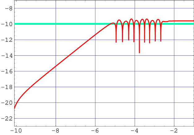
Finally, we show the evolution of the baryon asymmetry obtained by a numerical calculation in Fig. 3.9. From this figure we see that the asymmetry begins to oscillate with almost constant amplitude at and it is fixed at the time when the field starts to oscillate around the origin, . We also see that the amount of generated baryon asymmetry agrees well with our analytic estimation in Eq. (3.114). We confirm from this figure that the resultant asymmetry is well explained by the arguments described in this subsection.
3.4.4 Conditions to avoid an early oscillation
So far, we have neglected the thermal effects and assumed that there is no early oscillation, i.e., . If the field starts its oscillation before , i.e., if , the resultant baryon asymmetry is strongly suppressed. (In this case, the resultant baryon asymmetry is inversely proportional to .) Thus, we verify the assumption here.
First, in order to avoid the early oscillation caused by the soft SUSY breaking mass and the -term, we need
| (3.115) |
Next, the thermal mass term discussed in Sec. 3.2.3 may cause the early oscillation. This can be avoided if the following condition is satisfied:
| (3.116) |
Finally, we need the following third condition to avoid the early oscillation caused by the thermal log term , which was also explained in Sec. 3.2.3:
| (3.117) |
Here, we have used for .
From the second (3.116) and third (3.117) conditions, the reheating temperature is bounded from above as 242424At first sight, Eq. (3.118) seems to be obtained just by rewriting the relation by using the formula of in Eq. (3.38). However, it is slightly different, since takes a constant value for in the present case, while in the previous case.
| (3.118) |
where
| (3.119) |
We show the allowed regions which are free from the early oscillation in Fig. 3.10, taking account the conditions in Eqs. (3.115) and (3.118). From this figure, we see that the early oscillations can be easily avoided, especially when the breaking scale satisfies .
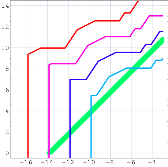
3.5 The neutrino-less double-beta decay
In Sec. 3.2, we have investigated the leptogenesis via flat direction in detail and have found that the produced baryon asymmetry is determined almost independently of the reheating temperature , because of the early oscillation of the flat direction field caused by thermal effects. As shown there, an ultralight neutrino is required to explain the empirical baryon asymmetry , except for the case where the model in Sec. 3.3.2 is adopted.252525See also the last comment in Sec. 3.2.4. By introducing a gauged symmetry, the early oscillation of the flat direction due to the thermal effect can be avoided (Sec. 3.4), but small neutrino mass is still necessary if we require low enough reheating temperature to avoid the cosmological gravitino problem in a wide range of gravitino mass (see Fig. 3.10). In this section we show that such a tiny mass of the lightest neutrino mass have an interesting implication on a low-energy experiment; the neutrino-less double beta () decay, which will be a strong evidence for the lepton number violation if observed.
The crucial parameter to determine the decay rate is the – component of the neutrino mass matrix, which is given by
| (3.120) |
where the mixing matrix is defined in Sec. 2.1. If the mass of the lightest neutrino is actually so small as , the contribution from to can be neglected as long as we consider an accessible decay rate, which corresponds to . Thus, the parameter is written in terms of masses and mixings of two other neutrinos as
| (3.121) |
which immediately leads to the following upper and lower bounds:
| (3.122) |
In general, the mass pattern of the neutrinos can be classified into two cases: the normal hierarchy and the inverted hierarchy. Let us consider these two cases in turn.
normal mass hierarchy
In the case of normal mass hierarchy, the parameters of atmospheric and solar neutrino oscillations are given by
| (3.123) |
and the mixing angle constrained by CHOOZ experiment [116] corresponds to , which is severely bounded as . In terms of these oscillation parameters, Eqs. (3.122) become
| (3.124) |
where and . Here, we can safely neglect the contribution of in the second term , since it changes at most .
Then, the ratio of the mass parameter to the mass scale of atmospheric neutrino oscillation is given by
| (3.125) |
Fig. 3.11 shows the upper and lower bounds on in units of , for , , and . As can be seen in Fig. 3.11, the mass parameter is predicted in a narrow range. We stress that this is because of the absence of the contribution from the lightest neutrino, i.e., . It is quite interesting to see that the predicted can be as large as –, which could be accessible at future decay experiments [120]. Furthermore, it is also found from Fig. 3.11 that, if the becomes more constrained by future experiments, is predicted in a much narrower range.
\psfrag{xxx}[c][c][0.6][0]{$\sin^{2}\theta_{\rm sol}\sqrt{{\displaystyle\frac{\delta m_{\rm sol}^{2}}{\delta m_{\rm atm}^{2}}}}$}\psfrag{mee}[c][c][0.6][-90]{${\displaystyle\frac{|m_{ee}|}{\sqrt{\delta m_{\rm atm}^{2}}}}$}\psfrag{chooz015}[r][r][0.5][0]{$\sin\theta_{\rm chooz}=\ 0.15$}\psfrag{chooz010}[r][r][0.5][0]{$0.10$}\psfrag{chooz005}[r][r][0.5][0]{$0.05$}\psfrag{chooz000}[r][r][0.5][0]{$0$}\includegraphics{Figs/mee-normal.eps}
\psfrag{xxx}[c][c][0.6][0]{$\tan^{2}\theta_{\rm sol}$}\psfrag{mee}[c][c][0.6][-90]{${\displaystyle\frac{|m_{ee}|}{\sqrt{\delta m_{\rm atm}^{2}}}}$}\includegraphics{Figs/mee-inverted.eps}
inverted hierarchy
Now let us turn to discuss the case of inverted mass hierarchy, where the parameters of atmospheric and solar neutrino oscillations are given by262626The convention adopted here is different from the one in Ref. [103], where are defined as for inverted hierarchy.
| (3.126) |
The mixing angle constrained by CHOOZ experiment [116] now corresponds to . Then from Eqs. (3.122) we obtain
| (3.127) |
In Fig. 3.12, we show the upper and lower bounds on in units of , for given . Here, we have used for simplicity, but changes (reduces) only 2% even for . As for the ratio , we have adopted – [10, 115]. As seen from the figure, the is restricted in a very narrow range such as – for , which is indeed in the reach of the future decay experiments [120].
The prediction of discussed in this section is a generic consequence of a hierarchical neutrino masses , . Thus the decay experiments, combined with neutrino oscillation experiments, can provide a consistency test for the tiny mass of the lightest neutrino required in the leptogenesis via flat direction.
3.A -flat condition for the flat direction
In this appendix, we discuss the -flat condition along the direction. Let us take the number of generations of the lepton doublets to be in general. Then, there are complex scalar fields in the - sector.
| (3.130) | |||||
| (3.133) |
First, the freedom to make gauge transformation allows us to rotate away a possible vacuum expectation value of one of the weak isospin components of one of the scalar fields. Thus, we can take without loss of generality. Then, vanishing -term potential requires the following relations:
| (3.134) | |||||
| (3.135) |
where the summations over are suppressed for simplicity. From these equations, the -flat condition is given by
| (3.136) |
It is still possible to rotate away one of the phases by using the gauge transformation (or third component of the gauge transformations272727Notice that one group remains unbroken by the condensation of the flat direction field.). Therefore, this flat “direction” is parameterized by [ complex fields] [one real constraint Eq. (3.136)] [one phase] real fields. In the absence of effective superpotential Eq. (3.2), this “direction” would be completely flat in the SUSY limit. Furthermore, it would be isotropic for directions, . However, due to the scalar potential induced by the operator Eq. (3.2), the potential is lifted and modified. Then, the flattest direction among the above field space is parameterized by one scalar field , which corresponds to the first family .
Chapter 4 Conclusions and discussion
| produced baryon asymmetry | ||
|---|---|---|
| thermal | ||
| inflaton decay | ||
| dominant | ||
| flat direction | ||
| – for | ||
| (See Fig. 3.4.) | ||
| gauged | ||
| -term stopping | ||
In this thesis, we have investigated various leptogenesis mechanisms in the framework of SUSY. We have also discussed some aspects of those scenarios, such as constraints from cosmological gravitino problems and possible experimental signatures. In particular, we have made essential improvements compared with earlier works in the following points:
-
•
In the leptogenesis scenario where the lepton asymmetry is created by the decay of right-handed sneutrino having dominated the early universe (Sec. 2.4), the dilution of the gravitino due to the entropy production by the ’s decay has been discussed. As a result, it has been shown that the cosmological gravitino problem is drastically ameliorated.
-
•
In the leptogenesis via the flat direction (Chapter 3), all the relevant thermal effects has been taken into account, and detailed analyses on the dynamics of the flat direction field has been done both by analytic and numerical calculations.
In this chapter, we summarize the aspects of various leptogenesis mechanisms investigated in this thesis. The produced baryon asymmetry in each mechanism is well summarized in Table 4.1.
First of all, we see that in all the mechanisms the neutrino mass plays a very crucial role to determine the resultant baryon asymmetry. In the mechanisms where lepton asymmetry is produced by the asymmetric decay of the right-handed (s)neutrino (Chapter 2), the asymmetry parameter is proportional to the mass of the heaviest neutrino for fixed effective -violating phase . We see that the information from the atmospheric neutrino oscillation [10], which leads to as long as masses of the light neutrinos are not degenerate, is very important to calculate the final baryon asymmetry. On the other hand, when the lepton asymmetry is produced via the flat direction (Chapter 3), the mass of the lightest neutrino is the crucial parameter.
It is interesting to see that the dependences on the neutrino masses are opposite in those two scenarios. As for the parameter of the right-handed neutrino decay, larger Yukawa coupling is favored to make larger. When we normalize the Yukawa couplings by neutrino masses (Sec. 2.1), turns out to be proportional to for fixed . On the other hand, for leptogenesis via flat direction, flatter direction is favored to enhance the final lepton asymmetry. This is because, the flatter the potential is, the larger the amplitude of becomes, and the larger the final lepton asymmetry is produced. Thus in this case the relevant neutrino mass is the lightest one, .
Now let us comment on each mechanism in turn.
thermal production of the right-handed (s)neutrino
The simplest one is the thermal production of the right-handed (s)neutrino (Sec. 2.2). The attractive point in this scenario is nothing but the fact that the production of the right-handed (s)neutrino requires no assumption besides high enough reheating temperature . The production occurs just by ordinary thermal scatterings.
On the other hand, since this scenario requires high enough reheating temperature, cosmological gravitino problems should be considered seriously. One solution is the stable (LSP) gravitino with mass . In this case, one has to take care of the decays of the next-to-lightest SUSY particle (NLSP) after the big-bang nucleosynthesis [20, 48], which gives severe constraints on the lifetime and the abundance of the NLSP at the decay. Since both of the lifetime and the abundance of the NLSP is determined by the properties of the NLSP (and the gravitino mass), they might be going to be well calculated if SUSY particles are discovered and their properties are studied in future collider experiments. This is quite an interesting possibility.
If the gravitino is not the LSP, cosmological gravitino problem is relatively severe. Therefore, it will be interesting and might be necessary to determine a definite lower bound on the reheating temperature at which the leptogenesis from thermally produced right-handed (s)neutrino works marginally. This requires to see what happens if the reheating temperature is just around the mass of the right-handed neutrino, .
leptogenesis in inflaton decay
The advantage of this mechanism is that the production of the right-handed (s)neutrino is possible for . Thus the cosmological gravitino problem can be avoided in a wider range of the gravitino mass. Actually, we have shown that the enough lepton asymmetry can be produced even with a reheating temperature . On the other hand, the produced baryon asymmetry crucially depends on the physics of the inflation. In particular, we have taken the branching ratio to be . In this sense the first one of the hybrid inflation models we have discussed in Sec. 2.3.3.a, which has Yukawa couplings between the inflaton and right-handed neutrinos, is attractive since it automatically gives rise to .
We should mention that the current and future satellite experiments on anisotropies of the cosmic microwave background radiation [90] will give precious information about the inflation physics, especially the spectrum index . Thus we will be able to distinguish which inflation model is favored by using future data.
-dominant universe
The resultant baryon asymmetry in this scenario is expressed in a very simple way, as given in Table 4.1. It is determined only by the decay temperature for fixed and . This is because the ’s decay produces dominant component of the radiation as well as the lepton asymmetry at once.
The most attractive feature of this scenario is the dilution of the gravitino. In fact, as we have shown, cosmological gravitino problems can be avoided even for , which is very special among other baryogenesis scenarios.
It is also quite an interesting possibility that the cosmic density perturbation coming from the ’s fluctuation might be detected at future experiments [99].
flat direction
We have performed a detailed analysis on this scenario, including all the relevant thermal effects. In spite of the complicated potential and dynamics of the flat direction field , it was shown that the result is very simple and attractive. The baryon asymmetry is determined almost only by the mass of the lightest neutrino . Remarkably, we can estimate (or predict) the from the empirical baryon asymmetry – as
| (4.1) |
almost independently of the reheating temperature for . It is amazing that the baryogenesis which happened in the very early universe is directly related to the neutrino mass.
flat direction gauged , -term stopping case
When we introduce an gauged symmetry, the dynamics of the flat direction field can be modified, if certain conditions are satisfied (-term stopping case). Then the resultant baryon asymmetry is enhanced compared with the case with -term stopping case, or the case without a gauged symmetry. Although the “reheating temperature independence” disappears in this case (and is no longer predicted), this scenario has an advantage in the case of gauge-mediated SUSY breaking (GMSB) models [45], compared to the previous case. The point is that the phase rotational motion of the field is provided not by the usual SUSY-breaking -term which is proportional to the gravitino mass, but by a Hubble-induced -term. Thus this mechanism can work even with a very light gravitino as in the GMSB models.
The neutrinoless double beta decay
We have also shown that a very light mass of the lightest neutrino , which is suggested by the above leptogenesis mechanisms via flat direction, leads to a high predictability of the rate of the neutrino-less double beta () decay. Although it is highly difficult to determine the mass of the lightest neutrino directly, future experiments on decay and neutrino oscillations will provide us precious information by which we can test the consistency of the very small lightest neutrino mass , as shown in Fig. 3.11 and 3.12.
Acknowledgement
I am very grateful to my advisor T. Yanagida for various instructive suggestions, stimulating discussions and collaborations, hearty encouragements and continuous support.
I would like to thank T. Asaka, M. Fujii, M. Kawasaki and H. Murayama, who are collaborators in various parts of this thesis, for fruitful discussions and collaborations.
I would also like to thank T. Watari for helpful discussions, and K. Ichikawa for helping me maintain the computer.
Finally, I thank all the members of particle physics theory group at University of Tokyo for their hospitality.
Appendix A Notations
We use natural units , where is the speed of light (in vacuum) and is the Planck constant. We also take the Boltzmann constant to be unity, which leads to .
denotes the reduced Planck scale, where is the Newton constant.
Throughout this thesis, except for generic discussions in Sec. 3.1, 3.2, 3.5 and 3.A, we assume the existence of the right-handed neutrinos, which have superpotentials:
| (A.1) |
where (), () and denote the supermultiplets of the heavy right-handed neutrinos, lepton doublets and the Higgs doublet which couples to up-type quarks, respectively.
We often use a basis where the mass matrix of the light neutrinos becomes diagonal, where the Yukawa couplings are given by . (The left subscript denotes the family of the heavy right-handed neutrinos , while the right subscript denotes the family of the light neutrinos in mass eigenstates. See Sec. 2.1 and Eq. (2.18).)
As for the parameters related to the cosmology, see next Appendix B.
Appendix B Some notes of standard cosmology
In this appendix, we briefly review some ingredients of the standard cosmology, in order to introduce our notations and relevant equations. For more details, see, for example, Ref. [28].
B.1 Friedmann-Robertson-Walker universe
The standard cosmology is based on the following homogeneous and isotropic metric (Robertson-Walker metric):
| (B.1) |
where is the “scale factor” of the expanding universe, and is the cosmic time. is called the comoving coordinates. From the above metric and the perfect-fluid form of the energy-momentum tensor ( and denote the energy density and the pressure, respectively), the Einstein equations lead to the following two equations:
| (B.2) | |||||
| (B.3) |
where the overdot denotes the derivative with cosmic time , and is the Newton constant.
The second equation (B.3), which corresponds to the conservation of the energy and momentum , describes the dilution of the energy density due to the expansion:
| (B.4) |
Notice that the above relations hold for each component of the energy density , as long as the energy-momentum conservation is satisfied separately for each .
The other equation (B.2), called Friedmann equation, describes the expansion of the universe. Notice that the curvature term decreases with time more slowly than the right-hand side of Eq. (B.2) as long as is dominated by matter () or radiation () [see Eq. (B.1)]. Therefore, it can be safely neglected as far as we consider the early universe.
The Hubble parameter is defined as
| (B.5) |
which means how fast the universe is expanding at a given stage of its expansion. In terms of this Hubble parameter , reduced Planck mass , critical energy density and density parameter , Eq. (B.2) is rewritten as follows:
| (B.6) |
Neglecting the curvature term, usually we use the following form of the Friedmann equation:
| (B.7) |
The present universe () observed is as follows [29]. The present Hubble expansion rate is , where , and hence critical energy density is . In terms of density parameter , total energy density is given by , which includes radiation ( is the number of the generations of neutrinos which are still relativistic today), matter (including baryon ) and “dark energy” .111The notation “” might not be correct, since the “dark energy” density could be a dynamical value (like “quintessence”), not a cosmological constant. For more details and the errors included in these values, see Ref. [29]. The nature of the cold dark matter (dominant component of the ) as well as that of the “dark energy” are big puzzles in cosmology, which is beyond the scope of this appendix. (As for the cold dark matter, however, supersymmetry provides a good candidate, the lightest SUSY particle (LSP). See also Sec. 2.4.3.)
From the above ratio of the present energy densities, it is found that the early universe was dominated by radiation (for ), and subsequently dominated by matter. Eqs. (B.1) and (B.7) lead to the following familiar relations for each epoch.222If we include the change of with time, which is defined below, the relation in Eq. (B.1) is slightly modified.
| (B.8) |
B.2 Thermodynamics
Here, we briefly review some basic thermodynamics in the radiation-dominated early universe, in which many particles are relativistic and in thermal equilibrium. First of all, the equilibrium density of particles of type with momenta in a range centered on is given by
| (B.9) |
where is the number of degrees of freedom and is the Fermi-Dirac or Bose-Einstein distribution function:
| (B.10) |
Here, is the energy , is the chemical potential of the particle , and the plus (minus) sign is for fermions (bosons). The number density , energy density and pressure of particle are then given by the following equations:
| (B.11) | |||||
| (B.12) | |||||
| (B.13) |
| fermion | boson | |
|---|---|---|
In Table B.1, we show these quantities for the relativistic () and non-relativistic () limits. Here, we have assumed and no Bose-Einstein condensation ().
Because the energy density of a non-relativistic particle is exponentially suppressed compared with the relativistic one, the total energy density of the radiation is given by the following simple form:
| (B.14) |
where
| (B.19) |
If there are particles which have different temperatures from that of the photon , another factor should be multiplied in the above expression. (For example, at , neutrinos have temperature for .)
Notice that all leptogenesis mechanisms discussed in this thesis work at temperatures far above the electroweak scale , where all the MSSM particles are expected to be in thermal equilibrium. In this case, we obtain
| (B.20) |
In the expanding universe, it is convenient to introduce the entropy density , which is defined by
| (B.21) | |||||
(Again, in the presence of particles with different temperatures, a factor of is multiplied in Eq. (B.21). In this case, the in Eq. (B.21) becomes slightly different from the in Eq. (B.14).) Notice that the entropy per comoving volume is conserved as far as no entropy production takes place. Thus it is quite convenient to take the ratio when we discuss some number density . For example, if some -number is conserved, the ratio of the -number density to the entropy density takes a constant value
| (B.22) |
as long as there is no entropy production, since both and scales as as the universe expands. As another example, if the -particle is in thermal equilibrium and relativistic (), the ratio is given by
| (B.23) |
where the temperature (or time) dependence only comes from .
Before closing this section, we calculate the relations between the particle number asymmetry and the particle’s chemical potential , which can be obtained by integrating Eq. (B.11). In order to calculate the asymmetry, it is necessary to calculate higher order terms than those in Table B.1. The results are given by
| (B.24) |
where ellipses denote higher order terms in the expansions of and . Here, we have assumed no Bose-Einstein condensation for boson, and relativistic limit . Eq. (B.24) is used in Sec. 1.4, in deriving the relation between the baryon and lepton asymmetries in the presence of sphaleron effect. In this case, the chemical potentials are of order , and hence the above assumptions are justified.
Bibliography
- [1] A. D. Sakharov, Pisma Zh. Eksp. Teor. Fiz. 5 (1967) 32 [JETP Lett. 5 (1967) 24].
-
[2]
M. Yoshimura,
Phys. Rev. Lett. 41 (1978) 281
[Erratum-ibid. 42 (1978) 746];
A. Y. Ignatev, N. V. Krasnikov, V. A. Kuzmin and A. N. Tavkhelidze, Phys. Lett. B 76 (1978) 436. -
[3]
D. Toussaint, S. B. Treiman, F. Wilczek and A. Zee,
Phys. Rev. D 19 (1979) 1036;
S. Weinberg, Phys. Rev. Lett. 42 (1979) 850;
M. Yoshimura, Phys. Lett. B 88 (1979) 294.
See also S. Dimopoulos and L. Susskind, Phys. Rev. D 18 (1978) 4500. -
[4]
H. Georgi and S. L. Glashow,
Phys. Rev. Lett. 32 (1974) 438;
J. C. Pati and A. Salam, Phys. Rev. D 10 (1974) 275. - [5] G. ’t Hooft, Phys. Rev. Lett. 37 (1976) 8; Phys. Rev. D 14 (1976) 3432 [Erratum-ibid. D 18 (1976) 2199].
- [6] V. A. Kuzmin, V. A. Rubakov and M. E. Shaposhnikov, Phys. Lett. B 155 (1985) 36.
- [7] A. G. Cohen, D. B. Kaplan and A. E. Nelson, Ann. Rev. Nucl. Part. Sci. 43 (1993) 27 [arXiv:hep-ph/9302210], and references therein.
-
[8]
For recent reviews and references, see, for example,
J. M. Cline, arXiv:hep-ph/9902328,
M. Quiros, Nucl. Phys. Proc. Suppl. 101 (2001) 401 [arXiv:hep-ph/0101230]. - [9] M. Fukugita and T. Yanagida, Phys. Lett. B174 (1986) 45.
-
[10]
Y. Fukuda et al. [Super-Kamiokande Collaboration],
Phys. Lett. B 433 (1998) 9 [arXiv:hep-ex/9803006];
Phys. Lett. B 436 (1998) 33 [arXiv:hep-ex/9805006];
Phys. Rev. Lett. 81 (1998) 1562 [arXiv:hep-ex/9807003].
See also a recent data,
T. Nakaya [SUPER-KAMIOKANDE Collaboration], arXiv:hep-ex/0209036. -
[11]
Y. Fukuda et al. [Super-Kamiokande Collaboration],
Phys. Rev. Lett. 81 (1998) 1158 [Erratum-ibid. 81 (1998) 4279] [arXiv:hep-ex/9805021];
Phys. Rev. Lett. 82 (1999) 2430 [arXiv:hep-ex/9812011];
Phys. Rev. Lett. 82 (1999) 1810 [arXiv:hep-ex/9812009];
Q. R. Ahmad et al. [SNO Collaboration], Phys. Rev. Lett. 87 (2001) 071301 [arXiv:nucl-ex/0106015];
B. T. Cleveland et al., Astrophys. J. 496 (1998) 505;
V. N. Gavrin [SAGE Collaboration], Nucl. Phys. Proc. Suppl. 91 (2001) 36;
E. Bellotti, Nucl. Phys. Proc. Suppl. 91 (2001) 44. - [12] K. Eguchi et al., [KamLAND Collaboration], arXiv:hep-ex/0212021.
-
[13]
T. Yanagida,
in Proceedings of the
“Workshop on the Unified Theory and the Baryon Number in the
Universe”, Tsukuba, Japan, 1979,
edited by O. Sawada and A. Sugamoto, KEK Report No. KEK-79-18, p. 95;
Prog. Theor. Phys. 64 (1980) 1103;
M. Gell-Mann, P. Ramond and R. Slansky, in “Supergravity”, edited by D.Z. Freedman and P. van Nieuwenhuizen (North-Holland, Amsterdam, 1979). -
[14]
J. Wess and B. Zumino,
Nucl. Phys. B 70 (1974) 39.
For a review and references of the supersymmetric extension of the standard model, see, for example, S. P. Martin, arXiv:hep-ph/9709356. -
[15]
J. R. Ellis, S. Kelley and D. V. Nanopoulos,
Phys. Lett. B 260 (1991) 131;
U. Amaldi, W. de Boer and H. Furstenau, Phys. Lett. B 260 (1991) 447;
P. Langacker and M. x. Luo, Phys. Rev. D 44 (1991) 817;
C. Giunti, C. W. Kim and U. W. Lee, Mod. Phys. Lett. A 6 (1991) 1745. -
[16]
N. Sakai,
Z. Phys. C 11 (1981) 153;
S. Dimopoulos and H. Georgi, Nucl. Phys. B 193 (1981) 150. -
[17]
K. Inoue, A. Kakuto, H. Komatsu and S. Takeshita,
Prog. Theor. Phys. 68 (1982) 927
[Erratum-ibid. 70 (1982) 330].
L. E. Ibanez and G. G. Ross, Phys. Lett. B 110 (1982) 215. - [18] For a review and references, see, G. Jungman, M. Kamionkowski and K. Griest, Phys. Rept. 267 (1996) 195 [arXiv:hep-ph/9506380].
-
[19]
M. Y. Khlopov and A. D. Linde,
Phys. Lett. B138 (1984) 265;
J. Ellis, J. E. Kim and D. V. Nanopoulos, Phys. Lett. B145 (1984) 181;
M. Kawasaki and T. Moroi, Prog. Theor. Phys. 93 (1995) 879 [arXiv:hep-ph/9403364].
see also a recent analysis,
M. Kawasaki, K. Kohri and T. Moroi, Phys. Rev. D 63 (2001) 103502 [arXiv:hep-ph/0012279]. -
[20]
T. Moroi, H. Murayama and M. Yamaguchi,
Phys. Lett. B 303 (1993) 289;
A. de Gouvea, T. Moroi and H. Murayama, Phys. Rev. D 56 (1997) 1281 [arXiv:hep-ph/9701244]. -
[21]
M. H. Reno and D. Seckel,
Phys. Rev. D 37 (1988) 3441;
S. Dimopoulos, R. Esmailzadeh, L. J. Hall and G. D. Starkman, Astrophys. J. 330 (1988) 545; Nucl. Phys. B 311 (1989) 699.
see also a recent analysis,
K. Kohri, Phys. Rev. D 64 (2001) 043515 [arXiv:astro-ph/0103411]. -
[22]
For recent reviews and references, see, for example,
M. Plumacher, Nucl. Phys. B 530 (1998) 207 [arXiv:hep-ph/9704231];
W. Buchmuller and M. Plumacher, Phys. Rept. 320 (1999) 329 [arXiv:hep-ph/9904310];
W. Buchmuller and M. Plumacher, Int. J. Mod. Phys. A 15 (2000) 5047 [arXiv:hep-ph/0007176]. -
[23]
K. Kumekawa, T. Moroi and T. Yanagida,
Prog. Theor. Phys. 92 (1994) 437
[arXiv:hep-ph/9405337];
G. Lazarides, Springer Tracts Mod. Phys. 163 (2000) 227 [arXiv:hep-ph/9904428] and references therein;
G. F. Giudice, M. Peloso, A. Riotto and I. Tkachev, JHEP 9908 (1999) 014 [arXiv:hep-ph/9905242];
T. Asaka, K. Hamaguchi, M. Kawasaki and T. Yanagida, Phys. Lett. B 464 (1999) 12 [arXiv:hep-ph/9906366], Phys. Rev. D 61 (2000) 083512 [arXiv:hep-ph/9907559];
M. Kawasaki, M. Yamaguchi and T. Yanagida, Phys. Rev. D 63 (2001) 103514 [arXiv:hep-ph/0011104]. - [24] H. Murayama, H. Suzuki, T. Yanagida and J. Yokoyama, Phys. Rev. Lett. 70 (1993) 1912.
- [25] H. Murayama and T. Yanagida, Phys. Lett. B 322 (1994) 349 [arXiv:hep-ph/9310297].
- [26] K. Hamaguchi, H. Murayama and T. Yanagida, Phys. Rev. D 65 (2002) 043512 [arXiv:hep-ph/0109030].
- [27] I. Affleck and M. Dine, Nucl. Phys. B 249 (1985) 361.
- [28] See, for example, E. Kolb and M. Turner, The Early Universe (Addison-Wisley, 1990).
- [29] D. E. Groom et al. [Particle Data Group Collaboration], “Review of particle physics,” Eur. Phys. J. C 15 (2000) 1.
- [30] N. S. Manton, Phys. Rev. D 28 (1983) 2019.
- [31] F. R. Klinkhamer and N. S. Manton, Phys. Rev. D 30 (1984) 2212.
-
[32]
This solution was also found in the following papers in different
contexts:
R. F. Dashen, B. Hasslacher and A. Neveu, Phys. Rev. D 10 (1974) 4138;
J. Boguta, Phys. Rev. Lett. 50 (1983) 148;
J. Burzlaff, Nucl. Phys. B 233 (1984) 262;
P. Forgacs and Z. Horvath, Phys. Lett. B 138 (1984) 397. - [33] See also A. D. Linde, Phys. Lett. B 70 (1977) 306, where a possible unsuppression of the baryon number violation via the tunneling at was briefly commented, and S. Dimopoulos and L. Susskind, in Ref. [3], where it was pointed out that the wash-out of the baryon asymmetry due to the tunneling between the distinct vacua could be efficient at temperature higher than the electroweak scale.
- [34] P. Arnold and L. D. McLerran, Phys. Rev. D 36 (1987) 581.
- [35] H. V. Klapdor-Kleingrothaus, S. Kolb and V. A. Kuzmin, Phys. Rev. D 62 (2000) 035014 [arXiv:hep-ph/9909546], and references therein.
-
[36]
P. Arnold, D. Son and L. G. Yaffe,
Phys. Rev. D 55 (1997) 6264
[arXiv:hep-ph/9609481];
D. Bodeker, Phys. Lett. B 426 (1998) 351 [arXiv:hep-ph/9801430];
D. Bodeker, G. D. Moore and K. Rummukainen, Phys. Rev. D 61 (2000) 056003 [arXiv:hep-ph/9907545];
G. D. Moore, arXiv:hep-ph/0009161, and references therein. -
[37]
S. Y. Khlebnikov and M. E. Shaposhnikov,
Nucl. Phys. B308 (1988) 885;
J. A. Harvey and M. S. Turner, Phys. Rev. D 42 (1990) 3344. -
[38]
S. Y. Khlebnikov and M. E. Shaposhnikov,
Phys. Lett. B 387 (1996) 817
[arXiv:hep-ph/9607386];
M. Laine and M. E. Shaposhnikov, Phys. Rev. D 61 (2000) 117302 [arXiv:hep-ph/9911473], and references therein. - [39] T. Moroi, arXiv:hep-ph/9503210.
- [40] S. Weinberg, Phys. Rev. Lett. 48 (1982) 1303.
- [41] M. Bolz, A. Brandenburg and W. Buchmuller, Nucl. Phys. B 606 (2001) 518 [arXiv:hep-ph/0012052].
- [42] M. Kawasaki, K. Kohri and T. Moroi, in Ref. [19].
-
[43]
L. Randall and R. Sundrum,
Nucl. Phys. B 557 (1999) 79
[arXiv:hep-th/9810155];
G. F. Giudice, M. A. Luty, H. Murayama and R. Rattazzi, JHEP 9812 (1998) 027 [arXiv:hep-ph/9810442];
J. A. Bagger, T. Moroi and E. Poppitz, JHEP 0004 (2000) 009 [arXiv:hep-th/9911029]. - [44] K. Kohri, in Ref. [21].
-
[45]
M. Dine, A. E. Nelson and Y. Shirman,
Phys. Rev. D 51 (1995) 1362
[arXiv:hep-ph/9408384].
M. Dine, A. E. Nelson, Y. Nir and Y. Shirman, Phys. Rev. D 53 (1996) 2658 [arXiv:hep-ph/9507378].
For a review, see, for example, G. F. Giudice and R. Rattazzi, Phys. Rept. 322 (1999) 419 [arXiv:hep-ph/9801271]. -
[46]
Y. Nomura and T. Yanagida,
Phys. Lett. B 487 (2000) 140
[arXiv:hep-ph/0005211].
Y. Nomura and K. Suzuki, arXiv:hep-ph/0110040. - [47] H. Pagels and J. R. Primack, Phys. Rev. Lett. 48 (1982) 223.
-
[48]
M. Bolz, W. Buchmüller and M. Plümacher,
Phys. Lett. B 443 (1998) 209
[arXiv:hep-ph/9809381];
T. Gherghetta, G. F. Giudice and A. Riotto, Phys. Lett. B 446 (1999) 28 [arXiv:hep-ph/9808401];
T. Asaka, K. Hamaguchi and K. Suzuki, Phys. Lett. B 490 (2000) 136 [arXiv:hep-ph/0005136]. - [49] M. Kawasaki and T. Moroi, Phys. Lett. B 346 (1995) 27 [arXiv:hep-ph/9408321].
- [50] T. Asaka and T. Yanagida, Phys. Lett. B 494 (2000) 297 [arXiv:hep-ph/0006211].
- [51] M. Fujii and T. Yanagida, arXiv:hep-ph/0208191.
- [52] H. Fujisaki, K. Kumekawa, M. Yamaguchi and M. Yoshimura, Phys. Rev. D 54 (1996) 2494 [arXiv:hep-ph/9511381].
-
[53]
R. Kallosh, L. Kofman, A. D. Linde and A. Van Proeyen,
Phys. Rev. D 61 (2000) 103503
[arXiv:hep-th/9907124];
G. F. Giudice, I. Tkachev and A. Riotto, JHEP 9908 (1999) 009 [arXiv:hep-ph/9907510]. - [54] H. P. Nilles, M. Peloso and L. Sorbo, Phys. Rev. Lett. 87 (2001) 051302 [arXiv:hep-ph/0102264].
-
[55]
M. Flanz, E. A. Paschos and U. Sarkar,
Phys. Lett. B 345 (1995) 248
[Erratum-ibid. B 384 (1995) 487]
[arXiv:hep-ph/9411366];
L. Covi, E. Roulet and F. Vissani, Phys. Lett. B 384 (1996) 169 [arXiv:hep-ph/9605319];
W. Buchmuller and M. Plumacher, Phys. Lett. B 431 (1998) 354 [arXiv:hep-ph/9710460]. - [56] L. Covi, E. Roulet and F. Vissani, in Ref. [55]
- [57] B. A. Campbell, S. Davidson and K. A. Olive, Nucl. Phys. B 399 (1993) 111 [arXiv:hep-ph/9302223].
- [58] M. Plumacher, in Ref. [22].
- [59] Z. Maki, M. Nakagawa and S. Sakata, Prog. Theor. Phys. 28 (1962) 870.
- [60] W. Buchmuller and T. Yanagida, Phys. Lett. B 445 (1999) 399 [arXiv:hep-ph/9810308].
- [61] For a discussion and references, see A. Pilaftsis, Int. J. Mod. Phys. A 14 (1999) 1811 [arXiv:hep-ph/9812256].
- [62] M. A. Luty, Phys. Rev. D 45 (1992) 455.
- [63] W. Buchmuller, P. Di Bari and M. Plumacher, Nucl. Phys. B 643 (2002) 367 [arXiv:hep-ph/0205349]; Phys. Lett. B 547 (2002) 128 [arXiv:hep-ph/0209301]. See also P. Di Bari, arXiv:hep-ph/0211175.
- [64] A. D. Dolgov and Y. B. Zeldovich, Rev. Mod. Phys. 53 (1981) 1.
- [65] E. W. Kolb and S. Wolfram, Nucl. Phys. B 172 (1980) 224 [Erratum-ibid. B 195 (1980) 542].
- [66] W. Buchmuller, arXiv:hep-ph/0101102.
- [67] M. Fujii, K. Hamaguchi and T. Yanagida, Phys. Rev. D 65 (2002) 115012 [arXiv:hep-ph/0202210].
- [68] C. D. Froggatt and H. B. Nielsen, Nucl. Phys. B 147 (1979) 277.
- [69] W. Buchmuller and T. Yanagida, Phys. Lett. B 302 (1993) 240.
- [70] S. Davidson and A. Ibarra, Phys. Lett. B 535 (2002) 25 [arXiv:hep-ph/0202239].
- [71] T. Asaka, K. Hamaguchi, M. Kawasaki and T. Yanagida, in Ref. [23].
- [72] M. Kawasaki, M. Yamaguchi and T. Yanagida, Phys. Rev. Lett. 85 (2000) 3572 [arXiv:hep-ph/0004243].
- [73] M. Kawasaki, M. Yamaguchi and T. Yanagida, in Ref. [23].
- [74] G. F. Giudice, M. Peloso, A. Riotto and I. Tkachev, in Ref. [23].
- [75] M. Fukugita and T. Yanagida, Phys. Rev. D 42 (1990) 1285.
-
[76]
J. Sato and T. Yanagida,
Nucl. Phys. Proc. Suppl. 77 (1999) 293
[arXiv:hep-ph/9809307];
P. Ramond, Nucl. Phys. Proc. Suppl. 77 (1999) 3 [arXiv:hep-ph/9809401]. - [77] J. Sato and T. Yanagida, Phys. Lett. B 493 (2000) 356 [arXiv:hep-ph/0009205].
- [78] G. Lazarides, in Ref. [23].
- [79] G. R. Dvali, Q. Shafi and R. Schaefer, Phys. Rev. Lett. 73 (1994) 1886 [arXiv:hep-ph/9406319].
- [80] E. J. Copeland, A. R. Liddle, D. H. Lyth, E. D. Stewart and D. Wands, Phys. Rev. D 49 (1994) 6410 [arXiv:astro-ph/9401011].
-
[81]
C. Panagiotakopoulos,
Phys. Rev. D 55 (1997) 7335
[arXiv:hep-ph/9702433];
A. D. Linde and A. Riotto, Phys. Rev. D 56 (1997) 1841 [arXiv:hep-ph/9703209]. - [82] C. L. Bennett et al., Astrophys. J. 464 (1996) L1 [arXiv:astro-ph/9601067].
-
[83]
A. D. Linde,
Phys. Lett. B 108 (1982) 389;
A. Albrecht and P. J. Steinhardt, Phys. Rev. Lett. 48 (1982) 1220. - [84] K. I. Izawa and T. Yanagida, Phys. Lett. B 393 (1997) 331 [arXiv:hep-ph/9608359].
- [85] See, for example, A.D. Linde, Particle Physics and Inflationary Cosmology, (Harwood, Chur, Switzerland, 1990).
-
[86]
K. I. Izawa, M. Kawasaki and T. Yanagida,
Phys. Lett. B 411 (1997) 249
[arXiv:hep-ph/9707201];
T. Asaka, M. Kawasaki and M. Yamaguchi, Phys. Rev. D 61 (2000) 027303 [arXiv:hep-ph/9906365]. -
[87]
A. D. Linde,
Phys. Lett. B 327 (1994) 208
[arXiv:astro-ph/9402031];
A. Vilenkin, Phys. Rev. Lett. 72 (1994) 3137 [arXiv:hep-th/9402085]. - [88] K. I. Izawa, M. Kawasaki and T. Yanagida, Prog. Theor. Phys. 101 (1999) 1129 [arXiv:hep-ph/9810537].
-
[89]
N. Sakai, H. A. Shinkai, T. Tachizawa and K. i. Maeda,
Phys. Rev. D 53 (1996) 655
[Erratum-ibid. D 54 (1996) 2981]
[arXiv:gr-qc/9506068];
I. Cho and A. Vilenkin, Phys. Rev. D 56 (1997) 7621 [arXiv:gr-qc/9708005];
A. A. de Laix, M. Trodden and T. Vachaspati, Phys. Rev. D 57 (1998) 7186 [arXiv:gr-qc/9801016]. -
[90]
http://map.gsfc.nasa.gov/http://astro.estec.esa.nl/SA-general/Projects/Planck/ -
[91]
M. Yoshimura,
Prog. Theor. Phys. 94 (1995) 873
[arXiv:hep-th/9506176];
H. Fujisaki, K. Kumekawa, M. Yamaguchi and M. Yoshimura, Phys. Rev. D 53 (1996) 6805 [arXiv:hep-ph/9508378];
L. Kofman, A. D. Linde and A. A. Starobinsky, Phys. Rev. D 56 (1997) 3258 [arXiv:hep-ph/9704452], and references therein. -
[92]
J. Baacke, K. Heitmann and C. Patzold,
Phys. Rev. D 58 (1998) 125013
[arXiv:hep-ph/9806205];
P. B. Greene and L. Kofman, Phys. Lett. B 448 (1999) 6 [arXiv:hep-ph/9807339]. - [93] H. Murayama, H. Suzuki, T. Yanagida and J. Yokoyama, Phys. Rev. D 50 (1994) 2356 [arXiv:hep-ph/9311326].
- [94] T. Moroi, H. Murayama and M. Yamaguchi, in Ref. [20].
- [95] M. Fujii, K. Hamaguchi and T. Yanagida, Phys. Rev. D 63 (2001) 123513 [arXiv:hep-ph/0102187].
- [96] A. Hebecker, J. March-Russell and T. Yanagida, arXiv:hep-ph/0208249.
- [97] R. Allahverdi, B. A. Campbell and J. Ellis, Nucl. Phys. B579 (2000) 355 [arXiv:hep-ph/0001122].
-
[98]
A. Anisimov and M. Dine,
Nucl. Phys. B 619 (2001) 729
[arXiv:hep-ph/0008058].
See also, A. Anisimov, arXiv:hep-ph/0111233. - [99] T. Moroi and H. Murayama, arXiv:hep-ph/0211019.
- [100] T. Moroi and T. Takahashi, Phys. Lett. B 522 (2001) 215 [Erratum-ibid. B 539 (2002) 303] [arXiv:hep-ph/0110096]; Phys. Rev. D 66 (2002) 063501 [arXiv:hep-ph/0206026], and references therein.
- [101] T. Asaka, M. Fujii, K. Hamaguchi and T. Yanagida, Phys. Rev. D 62 (2000) 123514 [arXiv:hep-ph/0008041].
- [102] M. Fujii, K. Hamaguchi and T. Yanagida, Phys. Rev. D 65 (2002) 043511 [arXiv:hep-ph/0109154].
- [103] M. Fujii, K. Hamaguchi and T. Yanagida, Phys. Lett. B 538 (2002) 107 [arXiv:hep-ph/0203189].
- [104] M. Dine, L. Randall and S. Thomas, Phys. Rev. Lett. 75 (1995) 398 [arXiv:hep-ph/9503303]. Nucl. Phys. B 458 (1996) 291 [arXiv:hep-ph/9507453].
- [105] T. Moroi and H. Murayama, JHEP 0007 (2000) 009 [arXiv:hep-ph/9908223].
- [106] M. Fujii, K. Hamaguchi and T. Yanagida, Phys. Rev. D 64 (2001) 123526 [arXiv:hep-ph/0104186].
- [107] M. Fujii and K. Hamaguchi, Phys. Lett. B 525 (2002) 143 [arXiv:hep-ph/0110072]; Phys. Rev. D 66 (2002) 083501 [arXiv:hep-ph/0205044].
- [108] B. A. Campbell, S. Davidson and K. A. Olive, Phys. Lett. B 303 (1993) 63 [arXiv:hep-ph/9302222].
- [109] M. Senami and K. Yamamoto, Phys. Lett. B 524 (2002) 332 [arXiv:hep-ph/0105054].
- [110] M. Senami and K. Yamamoto, Phys. Rev. D 66, 035006 (2002) [arXiv:hep-ph/0205041]; arXiv:hep-ph/0210073.
- [111] M. K. Gaillard, H. Murayama and K. A. Olive, Phys. Lett. B 355 (1995) 71 [arXiv:hep-ph/9504307].
- [112] J. Grundberg, T. H. Hansson and U. Lindstrom, arXiv:hep-th/9510045.
- [113] A. de Gouvêa, T. Moroi and H. Murayama, in Ref. [20].
- [114] T. Asaka, Phys. Lett. B 521 (2001) 329 [arXiv:hep-ph/0110073].
-
[115]
V. Barger and D. Marfatia,
arXiv:hep-ph/0212126;
G. L. Fogli, E. Lisi, A. Marrone, D. Montanino, A. Palazzo and A. M. Rotunno, arXiv:hep-ph/0212127;
M. Maltoni, T. Schwetz and J. W. Valle, arXiv:hep-ph/0212129;
A. Bandyopadhyay, S. Choubey, R. Gandhi, S. Goswami and D. P. Roy, arXiv:hep-ph/0212146;
J. N. Bahcall, M. C. Gonzalez-Garcia and C. Pena-Garay, arXiv:hep-ph/0212147;
H. Nunokawa, W. J. C. Teves, R. Zukanovich Funchal, arXiv:hep-ph/0212202;
P. Aliani, V. Antonelli, M. Picariello, E. Torrente-Lujan arXiv:hep-ph/0212212. - [116] M. Apollonio et al., Phys. Lett. B466 (1999) 415 [arXiv:hep-ex/9907037].
- [117] R. D. Peccei and H. R. Quinn, Phys. Rev. Lett. 38 (1977) 1440; Phys. Rev. D 16 (1977) 1791.
- [118] See, for a review, J. E. Kim, Phys. Rept. 150 (1987) 1.
- [119] K. Rajagopal, M. S. Turner and F. Wilczek, Nucl. Phys. B 358 (1991) 447.
-
[120]
See, for the present status of the double beta decay experiments,
S. R. Elliott and P. Vogel, arXiv:hep-ph/0202264, and references therein.